On a mixed FEM and a FOSLS with $H^{-1}$ loads

Abstract.

We study variants of the mixed finite element method (mixed FEM) and the first-order system least-squares finite element (FOSLS) for the Poisson problem where we replace the load by a suitable regularization which permits to use $H^{-1}$ loads. We prove that any bounded $H^{-1}$ projector onto piecewise constants can be used to define the regularization and yields quasi-optimality of the lowest-order mixed FEM resp. FOSLS in weaker norms. Examples for the construction of such projectors are given. One is based on the adjoint of a weighted Clément quasi-interpolator. We prove that this Clément operator has second-order approximation properties. For the modified mixed method we show optimal convergence rates of a postprocessed solution under minimal regularity assumptions — a result not valid for the lowest-order mixed FEM without regularization. Numerical examples conclude this work.

1. Introduction

In this work we study a mixed finite element method (FEM) and a first-order least-squares FEM (FOSLS) for the Poisson problem with $H^{-1}(\Omega)$ loads where $H^{-1}(\Omega)$ denotes the topological dual of the Sobolev space $H_{0}^{1}(\Omega)$ and $\Omega\subset\mathbb{R}^{n}$ ($n=2,3$) denotes a bounded Lipschitz domain with polytopal boundary. Both numerical methods are based on the following first-order reformulation of the Poisson problem with homogeneous Dirichlet boundary conditions,

(1a) $$\operatorname{div}{\boldsymbol{\sigma}} =-f \text{in }\Omega,$$

(1b) $${\boldsymbol{\sigma}}-\nabla u =0 \text{in }\Omega,$$

(1c) $$u =0 \text{on }\Gamma:=\partial\Omega.$$

Given $f\in L^{2}(\Omega)$ the mixed FEM seeks $(u_{\mathcal{T}},{\boldsymbol{\sigma}}_{\mathcal{T}})\in W_{\mathcal{T}}\times\Sigma_{\mathcal{T}}$ such that

(2a) $$({\boldsymbol{\sigma}}_{\mathcal{T}}\hskip 1.42262pt,{\boldsymbol{\tau}})+(u_{\mathcal{T}}\hskip 1.42262pt,\operatorname{div}{\boldsymbol{\tau}}) \,=\, 0,$$

(2b) $$(\operatorname{div}{\boldsymbol{\sigma}}_{\mathcal{T}}\hskip 1.42262pt,v) \,=\, (-f\hskip 1.42262pt,v)$$

for all $(v,{\boldsymbol{\tau}})\in W_{\mathcal{T}}\times\Sigma_{\mathcal{T}}:=\mathcal{P}^{0}(\mathcal{T})\times\mathcal{RT}^{0}(\mathcal{T})$, where $\mathcal{T}$ denotes a shape-regular mesh of simplices of $\Omega$, $\mathcal{P}^{p}(\mathcal{T})$ denotes the space of $\mathcal{T}$-piecewise polynomials of degree less or equal to $p\in\mathbb{N}_{0}$ and $\mathcal{RT}^{0}(\mathcal{T})$ is the lowest-order Raviart–Thomas space. Given $f\in L^{2}(\Omega)$ the FOSLS seeks the minimizer of the $L^{2}(\Omega)$ residuals of (1a)–(1b) over the discrete space $U_{\mathcal{T}}\times\Sigma_{\mathcal{T}}=\mathcal{P}^{1}(\mathcal{T})\cap H_{0}^{1}(\Omega)\times\Sigma_{\mathcal{T}}$, i.e.,

(3) $$(u_{\mathcal{T}},{\boldsymbol{\sigma}}_{\mathcal{T}})=\operatorname*{arg\,min}_{(v,{\boldsymbol{\tau}})\in U_{\mathcal{T}}\times\Sigma_{\mathcal{T}}}\|\operatorname{div}{\boldsymbol{\tau}}+f\|^{2}+\|\nabla v-{\boldsymbol{\tau}}\|^{2}.$$

Both methods, (2) and (3), are not well defined for $f\in H^{-1}(\Omega)$. In the recent article [15] we proposed to replace the load in (3) by a suitable polynomial approximation. The very same ideas in the analysis can be applied for the mixed FEM (2). To describe the new variants, let $Q_{\mathcal{T}}^{\star}\colon H^{-1}(\Omega)\to\mathcal{P}^{0}(\mathcal{T})\subseteq H^{-1}(\Omega)$ denote a bounded projection operator, i.e.,

$$Q_{\mathcal{T}}^{\star}\phi=\phi\quad\text{for all }\phi\in\mathcal{P}^{0}(\mathcal{T})\qquad\text{and}\qquad\|Q_{\mathcal{T}}^{\star}\phi\|_{-1}\lesssim\|\phi\|_{-1}\quad\text{for all }\phi\in H^{-1}(\Omega).$$

The modified methods are defined as follows:
Modified mixed FEM: Given $f\in H^{-1}(\Omega)$ seek $(u_{\mathcal{T}},{\boldsymbol{\sigma}}_{\mathcal{T}})\in W_{\mathcal{T}}\times\Sigma_{\mathcal{T}}$ such that

(4a) $$({\boldsymbol{\sigma}}_{\mathcal{T}}\hskip 1.42262pt,{\boldsymbol{\tau}})+(u_{\mathcal{T}}\hskip 1.42262pt,\operatorname{div}{\boldsymbol{\tau}}) \,=\, 0,$$

(4b) $$(\operatorname{div}{\boldsymbol{\sigma}}_{\mathcal{T}}\hskip 1.42262pt,v) \,=\, (-Q_{\mathcal{T}}^{\star}f\hskip 1.42262pt,v)$$

for all $(v,{\boldsymbol{\tau}})\in W_{\mathcal{T}}\times\Sigma_{\mathcal{T}}$.
Modified FOSLS: Given $f\in H^{-1}(\Omega)$ solve

(5) $$(u_{\mathcal{T}},{\boldsymbol{\sigma}}_{\mathcal{T}})=\operatorname*{arg\,min}_{(v,{\boldsymbol{\tau}})\in U_{\mathcal{T}}\times\Sigma_{\mathcal{T}}}\|\operatorname{div}{\boldsymbol{\tau}}+Q_{\mathcal{T}}^{\star}f\|^{2}+\|\nabla v-{\boldsymbol{\tau}}\|^{2}.$$

In our recent work [15] we proved that the solution $(u_{\mathcal{T}},{\boldsymbol{\sigma}}_{\mathcal{T}})$ of (5) satisfies the error estimate

$$\|u-u_{\mathcal{T}}\|_{1}+\|{\boldsymbol{\sigma}}-{\boldsymbol{\sigma}}_{\mathcal{T}}\|\lesssim h^{s}\|f\|_{-1+s}$$

where $s\in[0,1]$ depends on $\Omega$ and the regularity of $f$, and $h$ is the maximum element diameter. A similar estimate may be derived for the solution of (4) following the techniques from [15], or the ones presented here, see Corollary 5 below.

In the article at hand we complement on our results from [15] in that we show quasi-optimality of both the modified methods (4) and (5): Let $(u,{\boldsymbol{\sigma}})\in H_{0}^{1}(\Omega)\times L^{2}(\Omega;\mathbb{R}^{d})$ denote the solution of (1). If $(u_{\mathcal{T}},{\boldsymbol{\sigma}}_{\mathcal{T}})\in W_{\mathcal{T}}\times\Sigma_{\mathcal{T}}$ denotes the solution of (4), then (see Theorem 3)

$$\|u-u_{\mathcal{T}}\|+\|{\boldsymbol{\sigma}}-{\boldsymbol{\sigma}}_{\mathcal{T}}\|\lesssim\min_{(v,{\boldsymbol{\tau}})\in W_{\mathcal{T}}\times\Sigma_{\mathcal{T}}}\|u-v\|+\|{\boldsymbol{\sigma}}-{\boldsymbol{\tau}}\|,$$

or if $(u_{\mathcal{T}},{\boldsymbol{\sigma}}_{\mathcal{T}})\in U_{\mathcal{T}}\times\Sigma_{\mathcal{T}}$ denotes the solution of (5), then (see Theorem 6)

$$\|u-u_{\mathcal{T}}\|_{1}+\|{\boldsymbol{\sigma}}-{\boldsymbol{\sigma}}_{\mathcal{T}}\|\lesssim\min_{(v,{\boldsymbol{\tau}})\in U_{\mathcal{T}}\times\Sigma_{\mathcal{T}}}\|u-v\|_{1}+\|{\boldsymbol{\sigma}}-{\boldsymbol{\tau}}\|.$$

The mixed FEM (2) and FOSLS (3) have been studied thoroughly and we refer the interested reader to [3, 16, 2] for an introduction, overview and further literature on these methods. A variant of the hybrid higher-order method (known as HHO) with $H^{-1}(\Omega)$ loads is introduced and analyzed in [12]. For further details on and constructions of different $H^{-1}(\Omega)$ projection operators onto piecewise polynomial spaces we refer to the recent work [10] where also various applications are discussed. In [19] a general theory for the approximation of rough linear functionals is developed.

Postprocessing schemes for the mixed method (2) are well known [22], and optimal convergence rates for higher-order elements can be shown, whereas the lowest-order case, as considered here, requires sufficiently regular solutions, see, e.g., [22, Theorem 2.1 and Remark 2.1]. In the work at hand we prove that the postprocessing scheme from [22] applied to solutions of the modified mixed FEM (4) yields optimal rates with only minimal regularity assumptions.

The analysis of the latter is based on the dual of a weighted Clément quasi-interpolator. The advantage of our proposed construction is that the Clément operator reconstructs an approximation with second-order approximation properties from an elementwise projection on constants. For an overview on Clément quasi-interpolators we refer to the works [8, 6] and for additional information and applications to [7]. As a side product of our analysis we obtain a result on the approximation by piecewise constants in the dual space of $H^{2}(\Omega)\cap H_{0}^{1}(\Omega)$ (Corollary 13).

Our results on quasi-optimality in weaker norms might also be of interest for the analysis of FOSLS for eigenvalue problems [1]. The authors of [21] define a superconvergent FEM based on the postprocessing technique from [22]. Our new findings for the postprocessing scheme (Section 4) could also improve the results from [21] for the lowest-order case.

In this article we only consider lowest-order discretizations, though, many results can be extended to the higher-order case. E.g., for the FOSLS we refer the reader to the very recent work [20, Remark 4.7]. We restrict the presentation to $n=2,3$ but note that our results are valid for $n=1$. The remainder of this work is organized as follows: Section 2 introduces some notation and contains the statement and proofs of the quasi-optimality results stated above. In Section 3 we study a weighted Clément quasi-interpolator and discuss some of its main properties. Optimal error estimates for the postprocessed solution of (4) and optimal $L^{2}(\Omega)$ error estimates for the scalar solution of (5) are given in Section 4. This article closes with various numerical experiments (Section 5).

2. Quasi-optimality

This section is devoted to the proof of quasi-optimality results of the modified variants (4) and (5) of the mixed FEM and FOSLS claimed in the introduction. Before we give details in Section 2.3 we recall some known properties of projection operators needed for the analysis in Section 2.2. The proof of quasi-optimality requires a $H^{-1}(\Omega)$ bounded projection operator and we also give an example of such an operator that is easy to implement.

2.1. Sobolev spaces

For a Lipschitz domain $K\subseteq\Omega$ we denote by $H^{k}(K)$, $H_{0}^{k}(K)$, $k\in\mathbb{N}$ the usual Sobolev spaces with norms $\|\cdot\|_{K,k}$. If $K=\Omega$ we simply write $\|\cdot\|_{k}$. The space $H_{0}^{1}(\Omega)$ is equipped with the norm $\|\cdot\|_{1}:=\|\nabla(\cdot)\|$ where $\|\cdot\|$ is the $L^{2}(\Omega)$ norm with inner product $(\cdot\hskip 1.42262pt,\cdot)$. Similarly, $\|\cdot\|_{K}$ is the $L^{2}(K)$ norm with inner product $(\cdot\hskip 1.42262pt,\cdot)_{K}$. Intermediate Sobolev spaces with index $s$ are defined by (real) interpolation, e.g., $\widetilde{H}^{s}(\Omega)=[L^{2}(\Omega),H_{0}^{1}(\Omega)]_{s}$, $H^{s}(\Omega)=[L^{2}(\Omega),H^{1}(\Omega)]_{s}$ with norm denoted by $\|\cdot\|_{s}$. Dual spaces of Sobolev spaces are understood with respect to the extended $L^{2}$ inner product, e.g, the dual of $H_{0}^{1}(\Omega)$ is denoted by $H^{-1}(\Omega)$ and equipped with the dual norm

$$\|\phi\|_{-1}=\sup_{0\neq v\in H_{0}^{1}(\Omega)}\frac{(\phi\hskip 1.42262pt,v)}{\|v\|_{1}}.$$

Note that $H^{-s}(\Omega)=(\widetilde{H}^{s}(\Omega))^{\prime}$ with norms $\|\cdot\|_{-s}$, $s\in(0,1)$.

2.2. Projection and interpolation operators

Let $\mathcal{T}$ denote a regular mesh of simplices of $\Omega$ with $h_{\mathcal{T}}\in L^{\infty}(\Omega)$ denoting the elementwise mesh-size function, $h_{\mathcal{T}}|_{T}=\mathrm{diam}(T)$ for $T\in\mathcal{T}$. With $\mathcal{V}$ we denote all vertices of $\mathcal{T}$ and $\mathcal{V}_{0}=\mathcal{V}\setminus\Gamma$ are the interior vertices. The set of $n+1$ vertices of an element $T\in\mathcal{T}$ is $\mathcal{V}_{T}$. The patch of all elements of $\mathcal{T}$ sharing a node $z\in\mathcal{V}$ is denoted by $\omega_{z}$ and $\Omega_{z}$ is used for the domain associated to $\omega_{z}$. The element patch $\omega_{T}$ is the union of all vertex patches $\omega_{z}$ with $z\in\mathcal{V}_{T}$ and $\Omega_{T}$ is the corresponding domain.

Let $\Pi_{\mathcal{T}}^{0}\colon L^{2}(\Omega)\to W_{\mathcal{T}}=\mathcal{P}^{0}(\mathcal{T})$ denote the $L^{2}(\Omega)$-orthogonal projection which has the first-order approximation property

$$\|(1-\Pi_{\mathcal{T}}^{0})\phi\|_{T}\lesssim h_{T}\|\nabla\phi\|_{T}\quad\text{for all }\phi\in H^{1}(T),\,T\in\mathcal{T}.$$

Here, and in the remainder, the notation $A\lesssim B$ means that there exists a generic constant, possibly depending on the shape-regularity constant $\kappa_{\mathcal{T}}$ and $\Omega$, such that $A\leq C\cdot B$. The notation $A\eqsim B$ means $A\lesssim B$ and $B\lesssim A$. The shape-regularity constant of a mesh $\mathcal{T}$ is given by

$$\kappa_{\mathcal{T}}=\max_{T\in\mathcal{T}}\frac{h_{T}^{n}}{|T|},$$

where $|\cdot|$ denotes the volume measure.

Recall that $\Sigma_{\mathcal{T}}=\mathcal{RT}^{0}(\mathcal{T})$ is the lowest-order Raviart–Thomas space. We denote by $\Pi_{\mathcal{T}}^{\mathcal{RT}}\colon\boldsymbol{H}(\operatorname{div};\Omega)\to\Sigma_{\mathcal{T}}$ the projector constructed in [11]. It has the following properties, see [11, Theorem 3.2], where $\mathcal{RT}^{0}(T)$ denotes the lowest-order Raviart–Thomas space on the element $T$.

(6a) $$\operatorname{div}\Pi_{\mathcal{T}}^{\mathcal{RT}}{\boldsymbol{\sigma}} =\Pi_{\mathcal{T}}^{0}\operatorname{div}{\boldsymbol{\sigma}}\quad\text{and}$$

(6b) $$\|{\boldsymbol{\sigma}}-\Pi_{\mathcal{T}}^{\mathcal{RT}}{\boldsymbol{\sigma}}\|^{2} \lesssim\sum_{T\in\mathcal{T}}\min_{{\boldsymbol{\tau}}\in\mathcal{RT}^{0}(T)}\|{\boldsymbol{\sigma}}-{\boldsymbol{\tau}}\|_{T}^{2}+\|h_{\mathcal{T}}(1-\Pi_{\mathcal{T}}^{0})\operatorname{div}{\boldsymbol{\sigma}}\|^{2}$$

and, in particular,

(6c) $$\|\Pi_{\mathcal{T}}^{\mathcal{RT}}{\boldsymbol{\sigma}}\|_{\boldsymbol{H}(\operatorname{div};\Omega)}^{2}:=\|\Pi_{\mathcal{T}}^{\mathcal{RT}}{\boldsymbol{\sigma}}\|^{2}+\|\operatorname{div}\Pi_{\mathcal{T}}^{\mathcal{RT}}{\boldsymbol{\sigma}}\|^{2}\lesssim\|{\boldsymbol{\sigma}}\|_{\boldsymbol{H}(\operatorname{div};\Omega)}^{2}$$

for all $${\boldsymbol{\sigma}}\in\boldsymbol{H}(\operatorname{div};\Omega)$$.

There are several possibilities to construct a bounded projection $Q_{\mathcal{T}}^{\star}\colon H^{-1}(\Omega)\to\mathcal{P}^{0}(\mathcal{T})$. We refer the interested reader to [10] for an overview on existing operators and the construction of a family of $H^{-1}(\Omega)$ projectors into polynomial spaces. Here, we follow the construction presented in [15] resp. [14, Section 2.4]. First, define the averaged Scott–Zhang-type quasi-interpolator $J^{\mathrm{SZ}}_{\mathcal{T}}\colon H_{0}^{1}(\Omega)\to\mathcal{P}^{1}(\mathcal{T})\cap H_{0}^{1}(\mathcal{T})$ by

$$J^{\mathrm{SZ}}_{\mathcal{T}}v=\sum_{z\in\mathcal{V}_{0}}(v\hskip 1.42262pt,\psi_{z})\eta_{z},$$

where $\{\eta_{z}\}_{z\in\mathcal{V}_{0}}$ is the nodal basis of $\mathcal{P}^{1}(\mathcal{T})\cap H_{0}^{1}(\Omega)$, i.e., $\eta_{z}(z^{\prime})=\delta_{z,z^{\prime}}$ for all $z,z^{\prime}\in\mathcal{V}_{0}$, and $\delta_{z,z^{\prime}}$ denotes the Kronecker-$\delta$ symbol. Furthermore, $\psi_{z}\in\mathcal{P}^{1}(\mathcal{T})$ with $\operatorname{supp}\psi_{z}\subseteq\overline{\Omega_{z}}$ denotes the bi-orthogonal dual basis function satisfying

$$(\psi_{z}\hskip 1.42262pt,\eta_{z^{\prime}})=\delta_{z,z^{\prime}}\quad\forall z,z^{\prime}\in\mathcal{V}_{0}.$$

An explicit representation is given by

$$\psi_{z}|_{\Omega_{z}}=\frac{1}{|\Omega_{z}|}\big{(}(n+1)(n+2)\eta_{z}-(n+1)\big{)}.$$

For $T\in\mathcal{T}$ define the bubble function $\eta_{\mathrm{b},T}:=c_{T}\prod_{z\in\mathcal{V}_{T}}\eta_{z}$ with $c_{T}$ chosen so that $(\eta_{\mathrm{b},T}\hskip 1.42262pt,1)=1$ and

$$B_{\mathcal{T}}v=\sum_{T\in\mathcal{T}}(v\hskip 1.42262pt,\chi_{T})\eta_{\mathrm{b},T},$$

where $\chi_{T}\in L^{\infty}(\Omega)$ denotes the characteristic function on $T\in\mathcal{T}$. It is straightforward to check that $B_{\mathcal{T}}$ is locally bounded, i.e.,

$$\|B_{\mathcal{T}}v\|_{T}\lesssim\|v\|_{T}\quad\text{for all }T\in\mathcal{T}\text{ and }v\in L^{2}(\Omega).$$

The operator

(7) $$Q^{\mathrm{Cl}}_{\mathcal{T}}:=\Pi_{\mathcal{T}}^{0}\big{(}J^{\mathrm{SZ}}_{\mathcal{T}}+B_{\mathcal{T}}(1-J^{\mathrm{SZ}}_{\mathcal{T}})\big{)}^{\prime}=\Pi_{\mathcal{T}}^{0}\big{(}(J^{\mathrm{SZ}}_{\mathcal{T}})^{\prime}+(1-J^{\mathrm{SZ}}_{\mathcal{T}})^{\prime}B_{\mathcal{T}}^{\prime}\big{)}\colon H^{-1}(\Omega)\to\mathcal{P}^{0}(\mathcal{T})$$

with

$$(J^{\mathrm{SZ}}_{\mathcal{T}})^{\prime}\phi=\sum_{z\in\mathcal{V}_{0}}(\phi\hskip 1.42262pt,\eta_{z})\psi_{z},\quad(B_{\mathcal{T}})^{\prime}\phi=\sum_{T\in\mathcal{T}}(\phi\hskip 1.42262pt,\eta_{\mathrm{b},T})\chi_{T}$$

has the following properties.

Proposition 1 ([14, Theorem 8]).

The operator defined in (7) satisfies

• $Q^{\mathrm{Cl}}_{\mathcal{T}}\phi=\phi$ for all $\phi\in\mathcal{P}^{0}(\mathcal{T})$,

• $\|(1-Q^{\mathrm{Cl}}_{\mathcal{T}})\phi\|_{-1}\lesssim\|h_{\mathcal{T}}\phi\|$ for all $\phi\in L^{2}(\Omega)$,

• $\|Q^{\mathrm{Cl}}_{\mathcal{T}}\phi\|_{-1}\lesssim\|\phi\|_{-1}$ for all $\phi\in H^{-1}(\Omega)$, and

• $\|Q^{\mathrm{Cl}}_{\mathcal{T}}\phi\|\lesssim\|\phi\|$ for all $\phi\in L^{2}(\Omega)$.

In particular, $Q_{\mathcal{T}}^{\star}=Q^{\mathrm{Cl}}_{\mathcal{T}}$ can be used in the modified schemes (4), (5). We further study this operator in Section 3 where we recall a relation of $J^{\mathrm{SZ}}_{\mathcal{T}}$ to the Clément interpolation operator with $0$-th order moments. This relation is also of practical interest as it simplifies the calculation of $Q^{\mathrm{Cl}}_{\mathcal{T}}$.

2.3. Analysis of the modified mixed FEM resp. FOSLS

We need the following observation.

Lemma 2.

Let $u\in H_{0}^{1}(\Omega)$. If $Q_{\mathcal{T}}^{\star}\colon H^{-1}(\Omega)\to W_{\mathcal{T}}\subseteq H^{-1}(\Omega)$ is a bounded projector, then,

$$\|(1-Q_{\mathcal{T}}^{\star})\Delta u\|_{-1}\lesssim\|\nabla u-{\boldsymbol{\tau}}\|\quad\text{for all }{\boldsymbol{\tau}}\in\Sigma_{\mathcal{T}}.$$

Proof.

Let ${\boldsymbol{\tau}}\in\boldsymbol{H}(\operatorname{div};\Omega)$ with $\operatorname{div}{\boldsymbol{\tau}}\in W_{\mathcal{T}}$ be arbitrary. Since $Q_{\mathcal{T}}^{\star}$ is a bounded projection we have that

$$\|(1-Q_{\mathcal{T}}^{\star})\Delta u\|_{-1} =\|(1-Q_{\mathcal{T}}^{\star})\operatorname{div}(\nabla u-{\boldsymbol{\tau}})\|_{-1}$$

$$\lesssim\|\operatorname{div}(\nabla u-{\boldsymbol{\tau}})\|_{-1}\leq\|\nabla u-{\boldsymbol{\tau}}\|,$$

where the last estimate follows from boundedness of $\operatorname{div}\colon L^{2}(\Omega;\mathbb{R}^{n})\to H^{-1}(\Omega)$. ∎

The following theorem is the first main result of this section.

Theorem 3.

Let $Q_{\mathcal{T}}^{\star}\colon H^{-1}(\Omega)\to W_{\mathcal{T}}\subseteq H^{-1}(\Omega)$ denote a bounded projection. Given $f\in H^{-1}(\Omega)$, let $(u,{\boldsymbol{\sigma}})\in H_{0}^{1}(\Omega)\times L^{2}(\Omega;\mathbb{R}^{n})$ denote the solution of (1). The unique solution $(u_{\mathcal{T}},{\boldsymbol{\sigma}}_{\mathcal{T}})\in W_{\mathcal{T}}\times\Sigma_{\mathcal{T}}$ of (4) satisfies

$$\|u-u_{\mathcal{T}}\|+\|{\boldsymbol{\sigma}}-{\boldsymbol{\sigma}}_{\mathcal{T}}\|\lesssim\min_{(v,{\boldsymbol{\tau}})\in W_{\mathcal{T}}\times\Sigma_{\mathcal{T}}}\|u-v\|+\|{\boldsymbol{\sigma}}-{\boldsymbol{\tau}}\|.$$

Proof.

Let $\widetilde{u}\in H_{0}^{1}(\Omega)$ denote the unique weak solution of

$$-\Delta\widetilde{u}=Q_{\mathcal{T}}^{\star}f,\quad\widetilde{u}|_{\Gamma}=0.$$

By the triangle inequality and $\|u\|_{1}=\|\Delta u\|_{-1}$ we have that

$$\|u-u_{\mathcal{T}}\|+\|{\boldsymbol{\sigma}}-{\boldsymbol{\sigma}}_{\mathcal{T}}\| \leq\|u-\widetilde{u}\|+\|\nabla u-\nabla\widetilde{u}\|+\|\widetilde{u}-u_{\mathcal{T}}\|+\|\nabla\widetilde{u}-{\boldsymbol{\sigma}}_{\mathcal{T}}\|$$

$$\lesssim\|(1-Q_{\mathcal{T}}^{\star})f\|_{-1}+\|\widetilde{u}-u_{\mathcal{T}}\|+\|\nabla\widetilde{u}-{\boldsymbol{\sigma}}_{\mathcal{T}}\|.$$

Employing the quasi-optimality of the mixed method with datum in $L^{2}(\Omega)$, see, e.g. [16], we get that

$$\|\widetilde{u}-u_{\mathcal{T}}\|+\|\nabla\widetilde{u}-{\boldsymbol{\sigma}}_{\mathcal{T}}\|\lesssim\min_{(v,{\boldsymbol{\tau}})\in W_{\mathcal{T}}\times\Sigma_{\mathcal{T}}}\|\widetilde{u}-v\|+\|\nabla\widetilde{u}-{\boldsymbol{\tau}}\|+\|Q_{\mathcal{T}}^{\star}f+\operatorname{div}{\boldsymbol{\tau}}\|.$$

Using the properties (6) of $\Pi_{\mathcal{T}}^{\mathcal{RT}}$ and $\operatorname{div}\nabla\widetilde{u}=-Q_{\mathcal{T}}^{\star}f\in W_{\mathcal{T}}$, we see that

$$\min_{{\boldsymbol{\tau}}\in\Sigma_{\mathcal{T}}}\|\nabla\widetilde{u}-{\boldsymbol{\tau}}\|^{2}+\|Q_{\mathcal{T}}^{\star}f+\operatorname{div}{\boldsymbol{\tau}}\|^{2} \lesssim\sum_{T\in\mathcal{T}}\min_{{\boldsymbol{\tau}}\in\mathcal{RT}^{0}(T)}\|\nabla\widetilde{u}-{\boldsymbol{\tau}}\|_{T}^{2}+\|h_{\mathcal{T}}(1-\Pi_{\mathcal{T}}^{0})Q_{\mathcal{T}}^{\star}f\|^{2}$$

$$\qquad+\|Q_{\mathcal{T}}^{\star}f+\operatorname{div}\Pi_{\mathcal{T}}^{\mathcal{RT}}\nabla\widetilde{u}\|^{2}$$

$$\leq\min_{{\boldsymbol{\tau}}\in\Sigma_{\mathcal{T}}}\|\nabla\widetilde{u}-{\boldsymbol{\tau}}\|^{2}.$$

Combining the estimates and using the triangle inequality as well as $\|u-\widetilde{u}\|_{1}=\|(1-Q_{\mathcal{T}}^{\star})f\|_{-1}$ we infer that

$$\|u-u_{\mathcal{T}}\|+\|{\boldsymbol{\sigma}}-{\boldsymbol{\sigma}}_{\mathcal{T}}\|\lesssim\|(1-Q_{\mathcal{T}}^{\star})f\|_{-1}+\min_{(v,{\boldsymbol{\tau}})\in W_{\mathcal{T}}\times\Sigma_{\mathcal{T}}}\|u-v\|+\|{\boldsymbol{\sigma}}-{\boldsymbol{\tau}}\|.$$

The proof is finished by applying Lemma 2. ∎

For the scheme (2) with $f\in L^{2}(\Omega)$ a quasi-best approximation in the form

(8) $$\|{\boldsymbol{\sigma}}-{\boldsymbol{\sigma}}_{\mathcal{T}}\|=\min_{{\boldsymbol{\tau}}\in\mathcal{RT}^{0}(\mathcal{T}),\,\operatorname{div}{\boldsymbol{\tau}}=\Pi_{\mathcal{T}}^{0}\operatorname{div}{\boldsymbol{\sigma}}}{}\|{\boldsymbol{\sigma}}-{\boldsymbol{\tau}}\|$$

where ${\boldsymbol{\sigma}}\in\boldsymbol{H}(\operatorname{div};\Omega)$ is the solution to (1) and $(u_{\mathcal{T}},{\boldsymbol{\sigma}}_{\mathcal{T}})\in W_{\mathcal{T}}\times\Sigma_{\mathcal{T}}$ is the solution of (2) is known, see, e.g. [3] or [11, Lemma 6.1]. Note that the infimum is taken over a restricted set. For the modified version of the mixed method we have the following variant.

Theorem 4.

Let $Q_{\mathcal{T}}^{\star}\colon H^{-1}(\Omega)\to W_{\mathcal{T}}\subseteq H^{-1}(\Omega)$ denote a bounded projection. Given $f\in H^{-1}(\Omega)$, let $(u,{\boldsymbol{\sigma}})\in H_{0}^{1}(\Omega)\times L^{2}(\Omega;\mathbb{R}^{n})$ denote the solution of (1). The unique solution $(u_{\mathcal{T}},{\boldsymbol{\sigma}}_{\mathcal{T}})\in W_{\mathcal{T}}\times\Sigma_{\mathcal{T}}$ of (4) satisfies

$$\|{\boldsymbol{\sigma}}-{\boldsymbol{\sigma}}_{\mathcal{T}}\|\lesssim\min_{{\boldsymbol{\tau}}\in\Sigma_{\mathcal{T}}}\|{\boldsymbol{\sigma}}-{\boldsymbol{\tau}}\|.$$

Proof.

Let $\widetilde{u}\in H_{0}^{1}(\Omega)$ solve $-\Delta\widetilde{u}=Q_{\mathcal{T}}^{\star}f$, $\widetilde{\boldsymbol{\sigma}}:=\nabla\widetilde{u}$ and note that with quasi-optimality (8) and (6)

$$\|\widetilde{\boldsymbol{\sigma}}-{\boldsymbol{\sigma}}_{\mathcal{T}}\|=\min_{{\boldsymbol{\tau}}\in\mathcal{RT}^{0}(\mathcal{T}),\,\operatorname{div}{\boldsymbol{\tau}}=\Pi_{\mathcal{T}}^{0}\operatorname{div}\widetilde{\boldsymbol{\sigma}}}{}\|\widetilde{\boldsymbol{\sigma}}-{\boldsymbol{\tau}}\|\leq\|\widetilde{\boldsymbol{\sigma}}-\Pi_{\mathcal{T}}^{\mathcal{RT}}\widetilde{\boldsymbol{\sigma}}\|\lesssim\min_{{\boldsymbol{\tau}}\in\Sigma_{\mathcal{T}}}\|\widetilde{\boldsymbol{\sigma}}-{\boldsymbol{\tau}}\|.$$

Employing the triangle inequality twice we see that

$$\|{\boldsymbol{\sigma}}-{\boldsymbol{\sigma}}_{\mathcal{T}}\|\lesssim\|{\boldsymbol{\sigma}}-\widetilde{\boldsymbol{\sigma}}\|+\min_{{\boldsymbol{\tau}}\in\Sigma_{\mathcal{T}}}\|\widetilde{\boldsymbol{\sigma}}-{\boldsymbol{\tau}}\|\lesssim\|{\boldsymbol{\sigma}}-\widetilde{\boldsymbol{\sigma}}\|+\min_{{\boldsymbol{\tau}}\in\Sigma_{\mathcal{T}}}\|{\boldsymbol{\sigma}}-{\boldsymbol{\tau}}\|.$$

The proof is concluded by observing that $\|{\boldsymbol{\sigma}}-\widetilde{\boldsymbol{\sigma}}\|=\|(1-Q_{\mathcal{T}}^{\star})f\|_{-1}$ and applying Lemma 2. ∎

To derive convergence rates we require additional regularity of the load and the regularity shift of the Poisson problem. Suppose that $u\in H_{0}^{1}(\Omega)$ is the solution of (1). Then, by elliptic regularity, see, e.g., [17, 9], there exists $s_{\Omega}\in(1/2,1]$ depending only on $\Omega$ such that

(9) $$\|u\|_{1+t}\lesssim\|\Delta u\|_{-1+t}$$

for all $t\in[0,s_{\Omega}]$ with $\Delta u\in H^{-1+t}(\Omega)$.

Corollary 5.

Under the assumptions of Theorem 3 suppose additionally that $f\in H^{-1+s}(\Omega)$ for some $s\in[0,1]$. Then,

$$\|u-u_{\mathcal{T}}\|+\|{\boldsymbol{\sigma}}-{\boldsymbol{\sigma}}_{\mathcal{T}}{}\|\lesssim h^{\min\{s,s_{\Omega}\}}\|f\|_{-1+\min\{s,s_{\Omega}\}}.$$

Proof.

Quasi-optimality of Theorem 3 and approximation properties of $\Pi_{\mathcal{T}}^{0}$ imply that

$$\|u-u_{\mathcal{T}}\|+\|{\boldsymbol{\sigma}}-{\boldsymbol{\sigma}}_{\mathcal{T}}\| \lesssim h\|\nabla u\|+\min_{{\boldsymbol{\tau}}\in\Sigma_{\mathcal{T}}}\|{\boldsymbol{\sigma}}-{\boldsymbol{\tau}}\|.$$

For the first term note that $\|\nabla u\|=\|f\|_{-1}$. The other term can be bounded as in [15, Theorem 15]. We give the details for the sake of completeness. Note that

$$\|{\boldsymbol{\sigma}}-{\boldsymbol{\tau}}\|\leq\|{\boldsymbol{\sigma}}-\widetilde{\boldsymbol{\sigma}}\|+\|\widetilde{\boldsymbol{\sigma}}-{\boldsymbol{\tau}}\|_{\quad}\forall{\boldsymbol{\tau}}\in\Sigma_{\mathcal{T}},$$

where $\widetilde{\boldsymbol{\sigma}}=\nabla\widetilde{u}$ and $\widetilde{u}\in H_{0}^{1}(\Omega)$ solves $\Delta\widetilde{u}=-Q_{\mathcal{T}}^{\star}f$. By the projection property we have $(1-Q_{\mathcal{T}}^{\star})Q^{\mathrm{Cl}}_{\mathcal{T}}f=0$. Then,

$$\|{\boldsymbol{\sigma}}-\widetilde{\boldsymbol{\sigma}}\|=\|(1-Q_{\mathcal{T}}^{\star})f\|_{-1}\lesssim\|(1-Q^{\mathrm{Cl}}_{\mathcal{T}})f\|_{-1}\lesssim h^{\min\{s,s_{\Omega}\}}\|f\|_{-1+\min\{s,s_{\Omega}\}}.$$

The last estimate follows by an interpolation argument and Proposition 1. Finally, using (6) and choosing ${\boldsymbol{\tau}}=\Pi_{\mathcal{T}}^{\mathcal{RT}}\widetilde{\boldsymbol{\sigma}}$ we obtain

$$\|\widetilde{\boldsymbol{\sigma}}-{\boldsymbol{\tau}}\|^{2}\lesssim\sum_{T\in\mathcal{T}}\min_{{\boldsymbol{\chi}}\in\mathcal{RT}^{0}(T)}\|\widetilde{\boldsymbol{\sigma}}-{\boldsymbol{\chi}}\|_{T}^{2}\lesssim\|{\boldsymbol{\sigma}}-\widetilde{\boldsymbol{\sigma}}\|^{2}+\|{\boldsymbol{\sigma}}-\Pi_{\mathcal{T}}^{0}{\boldsymbol{\sigma}}\|^{2}$$

by noting that $\mathcal{P}^{0}(T)^{n}\subseteq\mathcal{RT}^{0}(T)$. The first term on the right-hand side is estimated as before and for the remaining term we get together with approximation properties of piecewise constants and elliptic regularity that $\|{\boldsymbol{\sigma}}-\Pi_{\mathcal{T}}^{0}{\boldsymbol{\sigma}}\|\lesssim h^{\min\{s,s_{\Omega}\}}\|f\|_{-1+\min\{s,s_{\Omega}\}}$. This finishes the proof. ∎

Next, we analyze quasi-optimality of the modified FOSLS (5) in weaker norms. The proof of the following result is similar to the proof of Theorem 3.

Theorem 6.

Let $Q_{\mathcal{T}}^{\star}\colon H^{-1}(\Omega)\to W_{\mathcal{T}}\subseteq H^{-1}(\Omega)$ denote a bounded projection. Given $f\in H^{-1}(\Omega)$, let $(u,{\boldsymbol{\sigma}})\in H_{0}^{1}(\Omega)\times L^{2}(\Omega;\mathbb{R}^{n})$ denote the solution of (1). The unique solution $(u_{\mathcal{T}},{\boldsymbol{\sigma}}_{\mathcal{T}})\in U_{\mathcal{T}}\times\Sigma_{\mathcal{T}}$ of (5) satisfies

$$\|u-u_{\mathcal{T}}\|_{1}+\|{\boldsymbol{\sigma}}-{\boldsymbol{\sigma}}_{\mathcal{T}}\|\lesssim\min_{(v,{\boldsymbol{\tau}})\in U_{\mathcal{T}}\times\Sigma_{\mathcal{T}}}\|u-v\|_{1}+\|{\boldsymbol{\sigma}}-{\boldsymbol{\tau}}\|.$$

Proof.

We use the notation from the proof of Theorem (3). Let $\widetilde{u}\in H_{0}^{1}(\Omega)$ denote the weak solution of $\Delta\widetilde{u}=-Q_{\mathcal{T}}^{\star}f$. With the triangle inequality, $\|u-\widetilde{u}\|_{1}=\|(1-Q_{\mathcal{T}}^{\star})f\|_{-1}$, ${\boldsymbol{\sigma}}=\nabla u$, $\widetilde{\boldsymbol{\sigma}}=\nabla\widetilde{u}$, and the quasi-optimality of the FOSLS in the canonic norms we get

$$\|u-u_{\mathcal{T}}\|_{1}+\|{\boldsymbol{\sigma}}-{\boldsymbol{\sigma}}_{\mathcal{T}}\| \lesssim\|(1-Q_{\mathcal{T}}^{\star})f\|_{-1}+\min_{(v,{\boldsymbol{\tau}})\in U_{\mathcal{T}}\times\Sigma_{\mathcal{T}}}\|\widetilde{u}-v\|_{1}+\|\widetilde{\boldsymbol{\sigma}}-{\boldsymbol{\tau}}\|+\|Q_{\mathcal{T}}^{\star}f+\operatorname{div}{\boldsymbol{\tau}}\|.$$

We argue as in the proof of Theorem 3 and obtain

$$\min_{{\boldsymbol{\tau}}\in\Sigma_{\mathcal{T}}}\|\widetilde{\boldsymbol{\sigma}}-{\boldsymbol{\tau}}\|+\|Q_{\mathcal{T}}^{\star}f+\operatorname{div}{\boldsymbol{\tau}}\|\lesssim\min_{{\boldsymbol{\tau}}\in\Sigma_{\mathcal{T}}}\|\nabla\widetilde{u}-{\boldsymbol{\tau}}\|\leq\|u-\widetilde{u}\|_{1}+\min_{{\boldsymbol{\tau}}\in\Sigma_{\mathcal{T}}}\|\nabla\widetilde{u}-{\boldsymbol{\tau}}\|.$$

Using $\|\widetilde{u}-v\|_{1}\leq\|u-v\|_{1}+\|u-\widetilde{u}\|_{1}=\|u-v\|_{1}+\|(1-Q_{\mathcal{T}}^{\star})f\|_{-1}$ and putting all the estimates together we infer

$$\|u-u_{\mathcal{T}}\|_{1}+\|{\boldsymbol{\sigma}}-{\boldsymbol{\sigma}}_{\mathcal{T}}\| \lesssim\|(1-Q_{\mathcal{T}}^{\star})f\|_{-1}+\min_{(v,{\boldsymbol{\tau}})\in U_{\mathcal{T}}\times\Sigma_{\mathcal{T}}}\|u-v\|_{1}+\|{\boldsymbol{\sigma}}-{\boldsymbol{\tau}}\|$$

and the proof is finished with an application of Lemma 2. ∎

Convergence rates in terms of powers of the maximum mesh-size $h$ for the modified FOSLS (5) have already been proved in [15, Theorem 15]. For completeness we recall the result.

Corollary 7.

Under the assumptions of Theorem 6 suppose additionally that $f\in H^{-1+s}(\Omega)$ for some $s\in[0,1]$. Then,

$$\|u-u_{\mathcal{T}}\|_{1}+\|{\boldsymbol{\sigma}}-{\boldsymbol{\sigma}}_{\mathcal{T}}{}\|\lesssim h^{\min\{s,s_{\Omega}\}}\|f\|_{-1+\min\{s,s_{\Omega}\}}.$$

3. Modified Clément quasi-interpolator

Define the Clément quasi-interpolator by

$$J^{\mathrm{Cl}}_{\mathcal{T}}v=\sum_{z\in\mathcal{V}_{0}}(v\hskip 1.42262pt,\chi_{z})\eta_{z}$$

with $0$-th order moments, i.e., $\chi_{z}\in\mathcal{P}^{0}(\mathcal{T})$ with $\operatorname{supp}(\chi_{z})\subseteq\overline{\Omega_{z}}$ and

$$\chi_{z}|_{\Omega_{z}}=\frac{1}{|\Omega_{z}|}.$$

This Clément quasi-interpolator has first-order approximation properties, i.e.,

$$\|v-J^{\mathrm{Cl}}_{\mathcal{T}}v\|_{T}\lesssim h_{T}\|\nabla v\|_{\Omega_{T}}.$$

It can be seen by noting that the operator reproduces constants on the patch $\omega_{z}$ at vertex $z\in\mathcal{V}_{0}$, see, e.g., [7]. However, the operator $J^{\mathrm{Cl}}_{\mathcal{T}}$, in general, does not have second-order approximation properties. Below we define a weighted Clément quasi-interpolator with second-order approximation properties.

There is a simple relation between $J^{\mathrm{SZ}}_{\mathcal{T}}$ and $J^{\mathrm{Cl}}_{\mathcal{T}}$, namely,

$$J^{\mathrm{SZ}}_{\mathcal{T}}\Pi_{\mathcal{T}}^{0}=J^{\mathrm{Cl}}_{\mathcal{T}},$$

see, [15, Lemma 21]. Together with $B_{\mathcal{T}}\Pi_{\mathcal{T}}^{0}=B_{\mathcal{T}}$ (which follows from the definition of $B_{\mathcal{T}}$) one sees that

$$Q^{\mathrm{Cl}}_{\mathcal{T}}=\Pi_{\mathcal{T}}^{0}\big{(}J^{\mathrm{SZ}}_{\mathcal{T}}+B_{\mathcal{T}}(1-J^{\mathrm{SZ}}_{\mathcal{T}})\big{)}^{\prime}=(J^{\mathrm{Cl}}_{\mathcal{T}})^{\prime}+(1-J^{\mathrm{Cl}}_{\mathcal{T}})^{\prime}B_{\mathcal{T}}^{\prime},$$

where

$$(J^{\mathrm{Cl}}_{\mathcal{T}})^{\prime}\phi=\sum_{z\in\mathcal{V}_{0}}(\phi\hskip 1.42262pt,\eta_{z})\chi_{z}.$$

If the mesh satisfies a certain symmetry condition, then it can be shown that $J^{\mathrm{Cl}}_{\mathcal{T}}$ also has second-order approximation properties although its argument is averaged over a nodal patch. To that end, given $T\in\mathcal{T}$ let $s_{T}=(n+1)^{-1}\sum_{z\in\mathcal{V}_{T}}z$ denote its center of mass. For any $z\in\mathcal{V}_{0}$ the centroid of its patch $\Omega_{z}$ is given by

$$s_{z}=\frac{1}{|\Omega_{z}|}\sum_{T\in\omega_{z}}|T|\,s_{T}.$$

The following result is found in [15, Lemma 22]:

Proposition 8.

If $s_{z}=z$ for all $z\in\mathcal{V}_{0}$, then

$$\|(1-J^{\mathrm{Cl}}_{\mathcal{T}})v\|\lesssim h^{2}\|D^{2}v\|\quad\text{for all }v\in H^{2}(\Omega)\cap H_{0}^{1}(\Omega).$$

The latter result is based on the observation that if $z=s_{z}$, then $J^{\mathrm{Cl}}_{\mathcal{T}}q(z)=q(z)$ for $q$ a polynomial of degree less or equal to one. This property is lost when $z\neq s_{z}$, see Section 5.1 for a numerical example. Particularly, we have that (following the proof of [15, Lemma 22]):

$$(J^{\mathrm{Cl}}_{\mathcal{T}}q)(z)=\frac{1}{|\Omega_{z}|}\int_{\Omega_{z}}q\,\mathrm{d}x=\frac{1}{|\Omega_{z}|}\sum_{T\in\omega_{z}}\int_{T}q\,\mathrm{d}x=\frac{1}{|\Omega_{z}|}\sum_{T\in\omega_{z}}|T|\,q(s_{T})=q(s_{z}).$$

For the construction of the weighted Clément quasi-interpolator consider for each $z\in\mathcal{V}_{0}$ a convex combination

(10) $$\sum_{T\in\omega_{z}}\alpha_{z,T}s_{T}=z,\quad\sum_{T\in\omega_{z}}\alpha_{z,T}=1,\quad\alpha_{z,T}\geq 0\quad(T\in\omega_{z}).$$

We stress that such a convex combination always exists, because $z$ lies in the convex hull of the center of masses $\{s_{T}\,:\,T\in\omega_{z}\}$, but for $n\geq 2$ it is not necessarily unique. Indeed, for each $z\in\mathcal{V}_{0}$ there are at least $n+1$ elements in $\omega_{z}$, but the node $z$ can be written as a convex combination of at most $n+1$ center of masses. We give two examples, one for $n=1$ and the other for $n=2$.

Example 9.

Let $\Omega=(a,b)$ and let $\mathcal{T}$ denote a partition of $\Omega$ into open intervals. For an interior node $z\in\mathcal{V}_{0}$ let $T_{z}^{-}=(z_{-},z)$ and $T_{z}^{+}=(z,z_{+})$ denote the two elements of the patch $\omega_{z}$. A straightforward computation shows that $\alpha_{z,T_{z}^{-}},\alpha_{z,T_{z}^{+}}$ satisfying (10) are unique and given by

$$\alpha_{z,T_{z}^{-}}=\frac{z_{+}-z}{z_{+}-z_{-}},\quad\alpha_{z,T_{z}^{+}}=\frac{z-z_{-}}{z_{+}-z_{-}}.$$

Example 10.

Consider $n=2$ and the nodes $z_{1}=(0,0)$, $z_{2}=(1,0)$, $z_{3}=(1,1)$, $z_{4}=(0,1)$ and $z=(\tfrac{1}{2},\tfrac{1}{3})$. The elements $T_{j}=\mathrm{conv}\{z_{j},z_{\!\!\mod(j,4)+1},z\}$, $j=1,2,3,4$, define a regular triangulation of the domain $\Omega=(0,1)^{2}$. The center of masses are given by

$$s_{T_{1}}=(\tfrac{1}{2},\tfrac{1}{9}),\quad s_{T_{2}}=(\tfrac{5}{6},\tfrac{4}{9}),\quad s_{T_{3}}=(\tfrac{1}{2},\tfrac{7}{9}),\quad s_{T_{4}}=(\tfrac{1}{6},\tfrac{4}{9}).$$

It can be verified that the convex combination (10) is not unique, e.g.,

$$\frac{2}{3}s_{T_{1}}+\frac{1}{3}s_{T_{3}}=z=\frac{1}{3}s_{T_{1}}+\frac{1}{3}s_{T_{2}}+\frac{1}{3}s_{T_{4}}.$$

For each $z\in\mathcal{V}_{0}$ let $(\alpha_{z,T})_{T\in\omega_{z}}$ denote fixed coefficients satisfying (10) and define

$$\varphi_{z}|_{T}=\begin{cases}\frac{\alpha_{z,T}}{|T|}&\text{if }T\in\omega_{z},\\ 0&\text{else}.\end{cases}$$

Thus, $\varphi_{z}\in\mathcal{P}^{0}(\mathcal{T})$ and $\|\varphi_{z}\|_{L^{\infty}(\Omega)}\eqsim|\Omega_{z}|^{-1}$. To see the latter equivalence note that $\alpha_{z,T}\leq 1$ for all $T\in\omega_{z}$, $z\in\mathcal{V}_{0}$. Therefore, $\|\varphi_{z}\|_{L^{\infty}(\Omega)}\lesssim|\Omega_{z}|^{-1}$. For the other bound, note that there exists at least one $T^{\star}\in\omega_{z}$ with $\alpha_{z,T^{\star}}\geq(\#\omega_{z})^{-1}$. Suppose this is not true, then $\sum_{T\in\omega_{z}}\alpha_{z,T}<\#\omega_{z}(\#\omega_{z})^{-1}=1$ which contradicts (10). We conclude that $\|\varphi_{z}\|_{L^{\infty}(\Omega)}\geq\alpha_{z,T^{\star}}|T^{\star}|^{-1}\gtrsim|\Omega_{z}|^{-1}$.

Let $\boldsymbol{\varphi}=\big{\{}\varphi_{z}\,:\,z\in\mathcal{V}_{0}\big{\}}$ denote the collection of all weight functions. The weighted Clément quasi-interpolator is given by

(11) $$J^{\mathrm{Cl},\boldsymbol{\varphi}}_{\mathcal{T}}v=\sum_{z\in\mathcal{V}_{0}}(v\hskip 1.42262pt,\varphi_{z})\eta_{z}\quad\text{for }v\in L^{1}(\Omega).$$

We collect its main properties in the next result.

Theorem 11.

The weighted Clément quasi-interpolator satisfies:

• $J^{\mathrm{Cl},\boldsymbol{\varphi}}_{\mathcal{T}}v=J^{\mathrm{Cl},\boldsymbol{\varphi}}_{\mathcal{T}}\Pi_{\mathcal{T}}^{0}v$ for all $v\in L^{2}(\Omega)$,

• $\|(1-J^{\mathrm{Cl},\boldsymbol{\varphi}}_{\mathcal{T}})v\|_{T}\lesssim h_{T}\|\nabla v\|_{\Omega_{T}}$ for all $T\in\mathcal{T}$ and $v\in H_{0}^{1}(\Omega)$,

• $\|(1-J^{\mathrm{Cl},\boldsymbol{\varphi}}_{\mathcal{T}})v\|_{T}\lesssim h_{T}^{2}\|D^{2}v\|_{\Omega_{T}}$ for all $T\in\mathcal{T}$ and $v\in H^{2}(\Omega)\cap H_{0}^{1}(\Omega)$,

• $\|J^{\mathrm{Cl},\boldsymbol{\varphi}}_{\mathcal{T}}v\|\lesssim\|v\|$ for all $v\in L^{2}(\Omega)$, resp. $\|J^{\mathrm{Cl},\boldsymbol{\varphi}}_{\mathcal{T}}v\|_{1}\lesssim\|v\|_{1}$ for all $v\in H_{0}^{1}(\Omega)$.

Proof.

To see the first assertion note that $\varphi_{z}\in\mathcal{P}^{0}(\mathcal{T})$, thus,

$$J^{\mathrm{Cl},\boldsymbol{\varphi}}_{\mathcal{T}}v=\sum_{z\in\mathcal{V}_{0}}(v\hskip 1.42262pt,\varphi_{z})\eta_{z}=\sum_{z\in\mathcal{V}_{0}}(v\hskip 1.42262pt,\Pi_{\mathcal{T}}^{0}\varphi_{z})\eta_{z}=\sum_{z\in\mathcal{V}_{0}}(\Pi_{\mathcal{T}}^{0}v\hskip 1.42262pt,\varphi_{z})\eta_{z}=J^{\mathrm{Cl},\boldsymbol{\varphi}}_{\mathcal{T}}\Pi_{\mathcal{T}}^{0}v.$$

Boundedness in $L^{2}(\Omega)$ follows from local boundedness. Let $T\in\mathcal{T}$ be given. We get with the usual scaling arguments together with $\|\varphi_{z}\|_{L^{\infty}(\Omega)}\lesssim|\Omega_{z}|^{-1}$ that

$$\|J^{\mathrm{Cl},\boldsymbol{\varphi}}_{\mathcal{T}}v\|_{T}\leq\sum_{z\in\mathcal{V}_{T}\cap\mathcal{V}_{0}}|(v\hskip 1.42262pt,\varphi_{z})|\,\|\eta_{z}\|_{T}\lesssim\sum_{z\in\mathcal{V}_{T}\cap\mathcal{V}_{0}}\|v\|_{\Omega_{z}}|\Omega_{z}|^{-1}\|1\|_{\Omega_{z}}|T|^{1/2}\lesssim\|v\|_{\Omega_{T}}.$$

The first-order and second-order approximation properties can be seen as follows. Let $q$ be a polynomial of degree less than or equal to one on $\Omega_{z}$. Then, for $z\in\mathcal{V}_{0}$ we have

$$J^{\mathrm{Cl},\boldsymbol{\varphi}}_{\mathcal{T}}q(z)=\int_{\Omega_{z}}\varphi_{z}q\,\mathrm{d}x =\sum_{T\in\omega_{z}}\frac{\alpha_{z,T}}{|T|}\int_{T}q\,\mathrm{d}x=\sum_{T\in\omega_{z}}\frac{\alpha_{z,T}}{|T|}|T|q(s_{T})$$

$$=\sum_{T\in\omega_{z}}\alpha_{z,T}\,q(s_{T})=q\Big{(}\sum_{T\in\omega_{z}}\alpha_{z,T}s_{T}\Big{)}=q(z).$$

Here, we used (10). Let $T\in\mathcal{T}$ be given and let $q$ denote a polynomial of degree less than or equal to one on $\Omega_{T}$ with $q(z)=0$ for $z\in\mathcal{V}_{T}\setminus\mathcal{V}_{0}$. With the aforegoing observations we see that $(J^{\mathrm{Cl},\boldsymbol{\varphi}}_{\mathcal{T}}q)(z)=q(z)$ for $z\in\mathcal{V}_{T}$ and, consequently, $J^{\mathrm{Cl},\boldsymbol{\varphi}}_{\mathcal{T}}q|_{T}=q|_{T}$. This and the local boundedness yield

$$\|(1-J^{\mathrm{Cl},\boldsymbol{\varphi}}_{\mathcal{T}})v\|_{T} =\|(1-J^{\mathrm{Cl},\boldsymbol{\varphi}}_{\mathcal{T}})(v-q)\|_{T}\lesssim\|v-q\|_{\Omega_{T}}.$$

The asserted approximation results then follow by a Bramble–Hilbert argument.

It remains to prove boundedness in $H_{0}^{1}(\Omega)$. Let $T\in\mathcal{T}$ be given and let $q$ denote a constant on $\Omega_{T}$ with $q(z)=0$ for $z\in\mathcal{V}_{T}\setminus\mathcal{V}_{0}$. Arguing as above we have $J^{\mathrm{Cl},\boldsymbol{\varphi}}_{\mathcal{T}}q|_{T}=q|_{T}$. The inverse estimate and local boundedness then show

$$\|\nabla J^{\mathrm{Cl},\boldsymbol{\varphi}}_{\mathcal{T}}v\|_{T} =\|\nabla J^{\mathrm{Cl},\boldsymbol{\varphi}}_{\mathcal{T}}(v-q)\|_{T}\lesssim h_{T}^{-1}\|J^{\mathrm{Cl},\boldsymbol{\varphi}}_{\mathcal{T}}(v-q)\|_{T}\lesssim h_{T}^{-1}\|v-q\|_{\Omega_{T}}.$$

Again, with a Bramble–Hilbert argument we conclude $h_{T}^{-1}\|v-q\|_{\Omega_{T}}\lesssim\|\nabla v\|_{\Omega_{T}}$, which finishes the proof. ∎

Following Section 2.2 we define a bounded projector $Q^{\mathrm{Cl},\boldsymbol{\varphi}}_{\mathcal{T}}\colon H^{-1}(\Omega)\to\mathcal{P}^{0}(\mathcal{T})$ based on the weighted Clément operator as

$$Q^{\mathrm{Cl},\boldsymbol{\varphi}}_{\mathcal{T}}:=(J^{\mathrm{Cl},\boldsymbol{\varphi}}_{\mathcal{T}})^{\prime}+(1-J^{\mathrm{Cl},\boldsymbol{\varphi}}_{\mathcal{T}})^{\prime}B_{\mathcal{T}}^{\prime}.$$

We summarize its properties in the next result. The proof follows similar as in [14, Theorem 8] and we only give some details:

Theorem 12.

The operator $Q^{\mathrm{Cl},\boldsymbol{\varphi}}_{\mathcal{T}}$ satisfies

• $Q^{\mathrm{Cl},\boldsymbol{\varphi}}_{\mathcal{T}}\phi=\phi$ for all $\phi\in\mathcal{P}^{0}(\mathcal{T})$,

• $\|(1-Q^{\mathrm{Cl},\boldsymbol{\varphi}}_{\mathcal{T}})\phi\|_{-1}\lesssim\|h_{\mathcal{T}}(1-\Pi_{\mathcal{T}}^{0})\phi\|$ for all $\phi\in L^{2}(\Omega)$,

• $\|Q^{\mathrm{Cl},\boldsymbol{\varphi}}_{\mathcal{T}}\phi\|_{-1}\lesssim\|\phi\|_{-1}$ for all $\phi\in H^{-1}(\Omega)$, and

• $\|Q^{\mathrm{Cl},\boldsymbol{\varphi}}_{\mathcal{T}}\phi\|\lesssim\|\phi\|$ for all $\phi\in L^{2}(\Omega)$.

Proof.

Using $J_{\mathcal{T}}=(Q^{\mathrm{Cl},\boldsymbol{\varphi}}_{\mathcal{T}})^{\prime}=J^{\mathrm{Cl},\boldsymbol{\varphi}}_{\mathcal{T}}+B_{\mathcal{T}}(1-J^{\mathrm{Cl},\boldsymbol{\varphi}}_{\mathcal{T}})$, boundedness of $B_{\mathcal{T}}$, and Theorem 11 we obtain

$$\|J_{\mathcal{T}}v\|\lesssim\|v\| \leq\|J^{\mathrm{Cl},\boldsymbol{\varphi}}_{\mathcal{T}}v\|+\|B_{\mathcal{T}}(1-J^{\mathrm{Cl},\boldsymbol{\varphi}}_{\mathcal{T}})v\|\lesssim\|v\|+\|(1-J^{\mathrm{Cl},\boldsymbol{\varphi}}_{\mathcal{T}})v\|\lesssim\|v\|.$$

The same arguments together with the inverse estimate and the approximation property of $J^{\mathrm{Cl},\boldsymbol{\varphi}}_{\mathcal{T}}$ prove that

$$\|\nabla J_{\mathcal{T}}v\|\lesssim\|\nabla v\|+\|h_{\mathcal{T}}^{-1}B_{\mathcal{T}}(1-J^{\mathrm{Cl},\boldsymbol{\varphi}}_{\mathcal{T}})v\|\lesssim\|\nabla v\|.$$

Therefore, $Q^{\mathrm{Cl},\boldsymbol{\varphi}}_{\mathcal{T}}=J_{\mathcal{T}}^{\prime}$ is bounded in $L^{2}(\Omega)$ resp. $H^{-1}(\Omega)$.

The projection property can be seen by noting that

$$(Q^{\mathrm{Cl},\boldsymbol{\varphi}}_{\mathcal{T}}\phi\hskip 1.42262pt,v)_{T}=(\phi\hskip 1.42262pt,J^{\mathrm{Cl},\boldsymbol{\varphi}}_{\mathcal{T}}+B_{\mathcal{T}}(1-J^{\mathrm{Cl},\boldsymbol{\varphi}}_{\mathcal{T}})v)_{T}=0$$

for all $\phi\in\mathcal{P}^{0}(\mathcal{T})$, $v\in L^{2}(\Omega)$.

Finally, the projection property and boundedness of $Q^{\mathrm{Cl},\boldsymbol{\varphi}}_{\mathcal{T}}$ yield

$$\|(1-Q^{\mathrm{Cl},\boldsymbol{\varphi}}_{\mathcal{T}})\phi\|_{-1}=\|(1-Q^{\mathrm{Cl},\boldsymbol{\varphi}}_{\mathcal{T}})(1-\Pi_{\mathcal{T}}^{0})\phi\|_{-1}\lesssim\|(1-\Pi_{\mathcal{T}}^{0})\phi\|_{-1}\lesssim\|h_{\mathcal{T}}(1-\Pi_{\mathcal{T}}^{0})\phi\|$$

for $\phi\in L^{2}(\Omega)$, which concludes the proof. ∎

The next result provides insight into the best-approximation of constants in the dual norm of $H^{2}(\Omega)\cap H_{0}^{1}(\Omega)$.

Corollary 13.

Let $X=H^{2}(\Omega)\cap H_{0}^{1}(\Omega)$. If $f\in L^{2}(\Omega)$, then

$$\min_{f_{\mathcal{T}}\in\mathcal{P}^{0}(\mathcal{T})}\|f-f_{\mathcal{T}}\|_{X^{\prime}}\leq\|(1-Q^{\mathrm{Cl},\boldsymbol{\varphi}}_{\mathcal{T}})f\|_{X^{\prime}}\lesssim\|h_{\mathcal{T}}^{2}(1-\Pi_{\mathcal{T}}^{0})f\|.$$

Proof.

Let $v\in H^{2}(\Omega)\cap H_{0}^{1}(\Omega)$. Then,

$$|((1-Q^{\mathrm{Cl},\boldsymbol{\varphi}}_{\mathcal{T}})f\hskip 1.42262pt,v)| =|((1-Q^{\mathrm{Cl},\boldsymbol{\varphi}}_{\mathcal{T}})(f-f_{\mathcal{T}})\hskip 1.42262pt,v)|$$

$$=|(f-f_{\mathcal{T}}\hskip 1.42262pt,(1-J^{\mathrm{Cl},\boldsymbol{\varphi}}_{\mathcal{T}})v-B_{\mathcal{T}}(1-J^{\mathrm{Cl},\boldsymbol{\varphi}}_{\mathcal{T}})v)|$$

$$\leq\sum_{T\in\mathcal{T}}\|f-f_{\mathcal{T}}\|_{T}\|(1-B_{\mathcal{T}})(1-J^{\mathrm{Cl},\boldsymbol{\varphi}}_{\mathcal{T}})v\|_{T}$$

$$\lesssim\sum_{T\in\mathcal{T}}\|f-f_{\mathcal{T}}\|_{T}\|(1-J^{\mathrm{Cl},\boldsymbol{\varphi}}_{\mathcal{T}})v\|_{T}$$

for all $f_{\mathcal{T}}\in\mathcal{P}^{0}(\mathcal{T})$. Here, we also used boundedness of $B_{\mathcal{T}}|_{T}\colon L^{2}(T)\to L^{2}(T)$. Applying Theorem 11 shows $\|(1-J^{\mathrm{Cl},\boldsymbol{\varphi}}_{\mathcal{T}})v\|_{T}\lesssim h_{T}^{2}\|D^{2}v\|_{\Omega_{T}}$. We conclude that

$$\|(1-Q^{\mathrm{Cl},\boldsymbol{\varphi}}_{\mathcal{T}})f\|_{X^{\prime}} =\sup_{v\in X\setminus\{0\}}\frac{((1-Q^{\mathrm{Cl},\boldsymbol{\varphi}}_{\mathcal{T}})f\hskip 1.42262pt,v)}{\|v\|_{\Omega,2}}\lesssim\|h_{\mathcal{T}}^{2}(1-\Pi_{\mathcal{T}}^{0})f\|.$$

This finishes the proof. ∎

4. $L^{2}$ estimates and postprocessed solution

In this section we revisit a well-known postprocessing scheme for mixed methods, see [22]. We show that using the operator $Q_{\mathcal{T}}^{\star}=Q^{\mathrm{Cl},\boldsymbol{\varphi}}_{\mathcal{T}}$ in (4) yields an improved result on the convergence of a postprocessed solution in the lowest-order case. It is known that the accuracy of postprocessed solutions $u_{\mathcal{T}}^{\star}$ hinges on a closeness result of the approximate solution, e.g., [22, Remark 2.1] notes that

$$\|\Pi_{\mathcal{T}}^{0}u-u_{\mathcal{T}}\|\lesssim h^{2}\|u\|_{3},$$

where $u_{\mathcal{T}}\in\mathcal{P}^{0}(\mathcal{T})$ is the solution of (2), to ensure that $\|u-u_{\mathcal{T}}^{\star}\|=\mathcal{O}(h^{2})$. The problem with this estimate is that it requires $u\in H^{3}(\Omega)$ or at least $u|_{T}\in H^{3}(T)$, $T\in\mathcal{T}$, which for $f\in L^{2}(T)\setminus H^{1}(T)$, $T\in\mathcal{T}$, is not realistic because even for the simplest model problem as considered in this work we can not expect more than $H^{2}(\Omega)$ regularity on convex domains.

For the analysis in this section we will use the solution $\widetilde{u}\in H_{0}^{1}(\Omega)$ of the auxiliary problem

(12) $$-\Delta\widetilde{u}=Q^{\mathrm{Cl},\boldsymbol{\varphi}}_{\mathcal{T}}f,\quad\text{and set }\widetilde{\boldsymbol{\sigma}}=\nabla\widetilde{u}.$$

4.1. Improved convergence of postprocessed solution

We start by analyzing a supercloseness property.

Lemma 14.

Let $f\in H^{-1+s}(\Omega)$ for some $s\in[0,1]$ and let $(u_{\mathcal{T}},{\boldsymbol{\sigma}}_{\mathcal{T}})\in W_{\mathcal{T}}\times\Sigma_{\mathcal{T}}$ denote the solution of (4) with $Q_{\mathcal{T}}^{\star}=Q^{\mathrm{Cl},\boldsymbol{\varphi}}_{\mathcal{T}}$. The estimate

$$\|\Pi_{\mathcal{T}}^{0}\widetilde{u}-u_{\mathcal{T}}\|\lesssim h^{s_{\Omega}}\|\widetilde{\boldsymbol{\sigma}}-{\boldsymbol{\sigma}}_{\mathcal{T}}\|\lesssim h^{s_{\Omega}+\min\{s,s_{\Omega}\}}\|f\|_{-1+\min\{s,s_{\Omega}\}}$$

holds, where $\widetilde{u}$ denotes the solution of (12) and $\widetilde{\boldsymbol{\sigma}}=\nabla\widetilde{u}$.

Proof.

The arguments used are essentially the same as in [22, Theorem 2.1] using the auxiliary solution $\widetilde{u}$ instead of $u$. Let $(v,{\boldsymbol{\tau}})\in H_{0}^{1}(\Omega)\times\boldsymbol{H}(\operatorname{div};\Omega)$ denote the unique solution of the first-order system,

$$\operatorname{div}{\boldsymbol{\tau}} =\Pi_{\mathcal{T}}^{0}\widetilde{u}-u_{\mathcal{T}},$$

$${\boldsymbol{\tau}}-\nabla v =0,$$

$$v|_{\Gamma} =0.$$

Elliptic regularity (9) shows

$$\|v\|_{1+s_{\Omega}}+\|{\boldsymbol{\tau}}\|_{s_{\Omega}}\lesssim\|\Pi_{\mathcal{T}}^{0}\widetilde{u}-u_{\mathcal{T}}\|_{-1+s_{\Omega}}\lesssim\|\Pi_{\mathcal{T}}^{0}\widetilde{u}-u_{\mathcal{T}}\|.$$

We have together with integration by parts that

$$\|\Pi_{\mathcal{T}}^{0}\widetilde{u}-u_{\mathcal{T}}\|^{2} =(\widetilde{u}-u_{\mathcal{T}}\hskip 1.42262pt,\Pi_{\mathcal{T}}^{0}\widetilde{u}-u_{\mathcal{T}})=(\widetilde{u}-u_{\mathcal{T}}\hskip 1.42262pt,\operatorname{div}{\boldsymbol{\tau}})$$

$$=(\widetilde{u}-u_{\mathcal{T}}\hskip 1.42262pt,\operatorname{div}{\boldsymbol{\tau}})+(\widetilde{\boldsymbol{\sigma}}-{\boldsymbol{\sigma}}_{\mathcal{T}}\hskip 1.42262pt,{\boldsymbol{\tau}}-\nabla v)$$

$$=(\widetilde{u}-u_{\mathcal{T}}\hskip 1.42262pt,\operatorname{div}{\boldsymbol{\tau}})+(\widetilde{\boldsymbol{\sigma}}-{\boldsymbol{\sigma}}_{\mathcal{T}}\hskip 1.42262pt,{\boldsymbol{\tau}})+(\operatorname{div}(\widetilde{\boldsymbol{\sigma}}-{\boldsymbol{\sigma}}_{\mathcal{T}})\hskip 1.42262pt,v)$$

$$=(\widetilde{u}-u_{\mathcal{T}}\hskip 1.42262pt,\operatorname{div}({\boldsymbol{\tau}}-{\boldsymbol{\tau}}_{\mathcal{T}}))+(\widetilde{\boldsymbol{\sigma}}-{\boldsymbol{\sigma}}_{\mathcal{T}}\hskip 1.42262pt,{\boldsymbol{\tau}}-{\boldsymbol{\tau}}_{\mathcal{T}})+(\operatorname{div}(\widetilde{\boldsymbol{\sigma}}-{\boldsymbol{\sigma}}_{\mathcal{T}})\hskip 1.42262pt,v)$$

for all ${\boldsymbol{\tau}}_{\mathcal{T}}\in\mathcal{RT}^{0}(\mathcal{T})$. The last identity follows from Galerkin orthogonality. Choosing ${\boldsymbol{\tau}}_{\mathcal{T}}=\Pi_{\mathcal{T}}^{\mathcal{RT}}{\boldsymbol{\tau}}$ we get that $\operatorname{div}({\boldsymbol{\tau}}-{\boldsymbol{\tau}}_{\mathcal{T}})=(1-\Pi_{\mathcal{T}}^{0})\operatorname{div}{\boldsymbol{\tau}}=0$ by (6) and noting that by (4) the equality $\operatorname{div}\widetilde{\boldsymbol{\sigma}}=-Q^{\mathrm{Cl},\boldsymbol{\varphi}}_{\mathcal{T}}f=\operatorname{div}{\boldsymbol{\sigma}}_{\mathcal{T}}$ holds, we further infer that

$$\|\Pi_{\mathcal{T}}^{0}\widetilde{u}-u_{\mathcal{T}}\|^{2} =(\widetilde{u}-u_{\mathcal{T}}\hskip 1.42262pt,\operatorname{div}({\boldsymbol{\tau}}-{\boldsymbol{\tau}}_{\mathcal{T}}))+(\widetilde{\boldsymbol{\sigma}}-{\boldsymbol{\sigma}}_{\mathcal{T}}\hskip 1.42262pt,{\boldsymbol{\tau}}-{\boldsymbol{\tau}}_{\mathcal{T}})+(\operatorname{div}(\widetilde{\boldsymbol{\sigma}}-{\boldsymbol{\sigma}}_{\mathcal{T}})\hskip 1.42262pt,v)$$

$$=(\widetilde{\boldsymbol{\sigma}}-{\boldsymbol{\sigma}}_{\mathcal{T}}\hskip 1.42262pt,{\boldsymbol{\tau}}-{\boldsymbol{\tau}}_{\mathcal{T}})\leq\|\widetilde{\boldsymbol{\sigma}}-{\boldsymbol{\sigma}}_{\mathcal{T}}\|\|{\boldsymbol{\tau}}-\Pi_{\mathcal{T}}^{\mathcal{RT}}{\boldsymbol{\tau}}\|$$

$$\lesssim\|\widetilde{\boldsymbol{\sigma}}-{\boldsymbol{\sigma}}_{\mathcal{T}}\|\left(\sum_{T\in\mathcal{T}}\min_{{\boldsymbol{\chi}}\in\mathcal{RT}^{0}(T)}\|{\boldsymbol{\tau}}-{\boldsymbol{\chi}}\|_{T}^{2}\right)^{1/2}\lesssim h^{s_{\Omega}}\|\widetilde{\boldsymbol{\sigma}}-{\boldsymbol{\sigma}}_{\mathcal{T}}\|\|\Pi_{\mathcal{T}}^{0}\widetilde{u}-u_{\mathcal{T}}\|.$$

The last estimate is a consequence of the fact that $\mathcal{P}^{0}(T)^{n}\subseteq\mathcal{RT}^{0}(T)$, the approximation property of piecewise constants and elliptic regularity.

It remains to prove $\|\widetilde{\boldsymbol{\sigma}}-{\boldsymbol{\sigma}}_{\mathcal{T}}\|\lesssim h^{\min\{s,s_{\Omega}\}}\|f\|_{-1+\min\{s,s_{\Omega}\}}$: The triangle inequality together with stability of the Poisson problem and quasi-optimality (Corollary 5) implies that

$$\|\widetilde{\boldsymbol{\sigma}}-{\boldsymbol{\sigma}}_{\mathcal{T}}\| \leq\|\nabla u-\nabla\widetilde{u}\|+\|{\boldsymbol{\sigma}}-{\boldsymbol{\sigma}}_{\mathcal{T}}\|$$

$$\lesssim\|(1-Q^{\mathrm{Cl},\boldsymbol{\varphi}}_{\mathcal{T}})f\|_{-1}+h^{\min\{s,s_{\Omega}\}}\|f\|_{-1+\min\{s,s_{\Omega}\}}.$$

From Theorem 12 we conclude $\|(1-Q^{\mathrm{Cl},\boldsymbol{\varphi}}_{\mathcal{T}})f\|_{-1}\lesssim h^{\min\{s,s_{\Omega}\}}\|f\|_{-1+\min\{s,s_{\Omega}\}}$ with an interpolation argument. This finishes the proof. ∎

We investigate the following postprocessing scheme, see, e.g. [22] for mixed schemes or [13] for the discontinuous Petrov–Galerkin method with optimal test functions. Let $(u_{\mathcal{T}},{\boldsymbol{\sigma}}_{\mathcal{T}})\in W_{\mathcal{T}}\times\Sigma_{\mathcal{T}}$ denote the solution of (4). Define $u_{\mathcal{T}}^{\star}\in\mathcal{P}^{1}(\mathcal{T})$ on each $T\in\mathcal{T}$ by

(13a) $$(\nabla u_{\mathcal{T}}^{\star}\hskip 1.42262pt,\nabla v)_{T} =({\boldsymbol{\sigma}}_{\mathcal{T}}\hskip 1.42262pt,\nabla v)_{T}\quad\forall v\in\mathcal{P}^{1}(T),$$

(13b) $$\Pi_{\mathcal{T}}^{0}u_{\mathcal{T}}^{\star}|_{T} =u_{\mathcal{T}}|_{T}.$$

Note that the postprocessing scheme from [22, Eq.(2.16)] is, in general, not well defined if $f\in H^{-1}(\Omega)\setminus L^{2}(\Omega)$. Replacing the load $f$ with $Q^{\mathrm{Cl},\boldsymbol{\varphi}}_{\mathcal{T}}f$ in [22, Eq.(2.16)] and using that $\operatorname{div}{\boldsymbol{\sigma}}_{\mathcal{T}}=-Q^{\mathrm{Cl},\boldsymbol{\varphi}}_{\mathcal{T}}f$ for the solution of (4) we get (13) after integrating by parts.

Theorem 15.

Let $f\in H^{-1+s}(\Omega)$ for some $s\in[0,1]$ and let $(u_{\mathcal{T}},{\boldsymbol{\sigma}}_{\mathcal{T}})\in W_{\mathcal{T}}\times\Sigma_{\mathcal{T}}$ denote the solution of (4) with $Q_{\mathcal{T}}^{\star}=Q^{\mathrm{Cl},\boldsymbol{\varphi}}_{\mathcal{T}}$. We have that

$$\|u-u_{\mathcal{T}}^{\star}\|\lesssim h^{s_{\Omega}+\min\{s,s_{\Omega}\}}\|f\|_{-1+\min\{s,s_{\Omega}\}}.$$

In particular, if $\Omega$ is convex and $f\in L^{2}(\Omega)$, then

$$\|u-u_{\mathcal{T}}^{\star}\|\lesssim h^{2}\|f\|.$$

Proof.

Using the triangle inequality and $\Pi_{\mathcal{T}}^{0}u_{\mathcal{T}}^{\star}=u_{\mathcal{T}}=\Pi_{\mathcal{T}}^{0}u_{\mathcal{T}}$ we get

(14) $$\begin{split}\|u-u_{\mathcal{T}}^{\star}\|&\leq\|u-\widetilde{u}\|+\|\widetilde{u}-u_{\mathcal{T}}^{\star}\|\\ &\leq\|u-\widetilde{u}\|+\|(1-\Pi_{\mathcal{T}}^{0})(\widetilde{u}-u_{\mathcal{T}}^{\star})\|+\|\Pi_{\mathcal{T}}^{0}(\widetilde{u}-u_{\mathcal{T}}^{\star})\|\\ &\lesssim\|u-\widetilde{u}\|+\left(\sum_{T\in\mathcal{T}}h_{T}^{2}\|\nabla(\widetilde{u}-u_{\mathcal{T}}^{\star})\|_{T}^{2}\right)^{1/2}+\|\Pi_{\mathcal{T}}^{0}\widetilde{u}-u_{\mathcal{T}}\|.\end{split}$$

The last term on the right-hand side is estimated with Lemma 14,

$$\|\Pi_{\mathcal{T}}^{0}\widetilde{u}-u_{\mathcal{T}}\|\lesssim h^{s_{\Omega}+\min\{s,s_{\Omega}\}}\|f\|_{-1+\min\{s,s_{\Omega}\}}.$$

For the first term on the right-hand side of (14) let $v\in H_{0}^{1}(\Omega)$ denote the solution of $-\Delta v=u-\widetilde{u}$. Then, with elliptic regularity and the properties of $Q^{\mathrm{Cl},\boldsymbol{\varphi}}_{\mathcal{T}}$ resp. $(Q^{\mathrm{Cl},\boldsymbol{\varphi}}_{\mathcal{T}})^{\prime}$ we infer that

$$\|u-\widetilde{u}\|^{2} =(u-\widetilde{u}\hskip 1.42262pt,-\Delta v)=((1-Q^{\mathrm{Cl},\boldsymbol{\varphi}}_{\mathcal{T}})f\hskip 1.42262pt,v)=((1-Q^{\mathrm{Cl},\boldsymbol{\varphi}}_{\mathcal{T}})f\hskip 1.42262pt,(1-(Q^{\mathrm{Cl},\boldsymbol{\varphi}}_{\mathcal{T}})^{\prime})v)$$

$$\lesssim\|(1-Q^{\mathrm{Cl},\boldsymbol{\varphi}}_{\mathcal{T}})f\|_{-1}\|(1-(Q^{\mathrm{Cl},\boldsymbol{\varphi}}_{\mathcal{T}})^{\prime})v\|_{1}\lesssim h^{\min\{s,s_{\Omega}\}}\|f\|_{-1+\min\{s,s_{\Omega}\}}h^{s_{\Omega}}\|v\|_{1+s_{\Omega}}$$

$$\lesssim h^{s_{\Omega}+\min\{s,s_{\Omega}\}}\|f\|_{-1+\min\{s,s_{\Omega}\}}\|u-\widetilde{u}\|.$$

The remaining term on the right-hand side of (14) is estimated following arguments similar as, e.g., found in [22, Proof of Theorem 2.2] or [13, Section 3.5]. For the sake of completeness we repeat the steps here. Let $\widetilde{u}_{\mathcal{T}}\in\mathcal{P}^{1}(\mathcal{T})$ denote the solution of the local Neumann problems

$$(\nabla\widetilde{u}_{\mathcal{T}}\hskip 1.42262pt,\nabla v)_{T} =(\widetilde{\boldsymbol{\sigma}}\hskip 1.42262pt,\nabla v)_{T}\quad\forall v\in\mathcal{P}^{1}(T),$$

$$(\widetilde{u}_{T}\hskip 1.42262pt,1)_{T} =0$$

for each $T\in\mathcal{T}$. Note that $\widetilde{u}_{\mathcal{T}}$ is the (elementwise) Galerkin approximation of $\widetilde{u}$. Therefore,

$$\|\nabla(\widetilde{u}-u_{\mathcal{T}}^{\star})\|_{T} \leq\|\nabla(\widetilde{u}-\widetilde{u}_{\mathcal{T}})\|_{T}+\|\nabla(\widetilde{u}_{\mathcal{T}}-u_{\mathcal{T}}^{\star})\|_{T}$$

$$\leq\|\nabla(\widetilde{u}-v)\|_{T}+\|\widetilde{\boldsymbol{\sigma}}-{\boldsymbol{\sigma}}_{\mathcal{T}}\|_{T}$$

for all $v\in\mathcal{P}^{1}(T)$. Multiplying by $h_{T}$, summing over all elements, and using the triangle inequality we conclude that

(15) $$\left(\sum_{T\in\mathcal{T}}h_{T}^{2}\|\nabla(\widetilde{u}-u_{\mathcal{T}}^{\star})\|_{T}^{2}\right)^{1/2} \lesssim h\|\nabla(u-\widetilde{u})\|+h\min_{v\in U_{\mathcal{T}}}\|u-v\|_{1}+h\|{\boldsymbol{\sigma}}-{\boldsymbol{\sigma}}_{\mathcal{T}}\|.$$

The first term on the right-hand side of (15) is estimated using stability of the Poisson problem and properties of $Q^{\mathrm{Cl},\boldsymbol{\varphi}}_{\mathcal{T}}$ leading to

$$h\|\nabla(u-\widetilde{u})\|\eqsim h\|(1-Q^{\mathrm{Cl},\boldsymbol{\varphi}}_{\mathcal{T}})f\|_{-1}\lesssim h^{1+\min\{s,s_{\Omega}\}}\|f\|_{-1+\min\{s,s_{\Omega}\}}.$$

For the remaining terms on the right-hand side of (15) we use Corollary 5 and Theorem 6 together with Corollary 7 to conclude that

$$h\min_{v\in U_{\mathcal{T}}}\|u-v\|_{1}+h\|{\boldsymbol{\sigma}}-{\boldsymbol{\sigma}}_{\mathcal{T}}\|\lesssim h^{1+\min\{s,s_{\Omega}\}}\|f\|_{-1+\min\{s,s_{\Omega}\}}.$$

Combining all estimates and using $h\lesssim h^{s_{\Omega}}$ finishes the proof. ∎

Another consequence of Lemma 14 is the following result.

Corollary 16.

Let $f\in H^{-1+s}(\Omega)$ for some $s\in[0,1]$ and let $(u_{\mathcal{T}},{\boldsymbol{\sigma}}_{\mathcal{T}})\in W_{\mathcal{T}}\times\Sigma_{\mathcal{T}}$ denote the solution of (4) with $Q_{\mathcal{T}}^{\star}=Q^{\mathrm{Cl},\boldsymbol{\varphi}}_{\mathcal{T}}$. We have that

$$\|u-u_{\mathcal{T}}\|\leq\|u-\Pi_{\mathcal{T}}^{0}u\|+Ch^{s_{\Omega}+\min\{s,s_{\Omega}\}}\|f\|_{-1+\min\{s,s_{\Omega}\}},$$

where $C>0$ denotes a generic constant.

Proof.

By the triangle inequality,

$$\|u-u_{\mathcal{T}}\| \leq\|u-\Pi_{\mathcal{T}}^{0}u\|+\|\Pi_{\mathcal{T}}(u-\widetilde{u})\|+\|\Pi_{\mathcal{T}}\widetilde{u}-u_{\mathcal{T}}\|$$

$$\leq\|u-\Pi_{\mathcal{T}}^{0}u\|+\|u-\widetilde{u}\|+\|\Pi_{\mathcal{T}}\widetilde{u}-u_{\mathcal{T}}\|.$$

The last term is estimated with Lemma 14 and the middle term is estimated as in the proof of Theorem 15. ∎

4.2. $L^{2}$ convergence of FOSLS

In this section we study the $L^{2}(\Omega)$ error $\|u-u_{\mathcal{T}}\|$, where $(u_{\mathcal{T}},{\boldsymbol{\sigma}}_{\mathcal{T}})\in U_{\mathcal{T}}\times\Sigma_{\mathcal{T}}$ is the solution to the modified FOSLS (5). For convex domains and $f\in L^{2}(\Omega)$ we already studied $L^{2}(\Omega)$ convergence rates in [15, Theorem 18] when using the operator $Q_{\mathcal{T}}^{\star}=Q^{\mathrm{Cl}}_{\mathcal{T}}$. The following theorem extends the findings of [15, Section 4] for $Q_{\mathcal{T}}^{\star}=Q^{\mathrm{Cl},\boldsymbol{\varphi}}_{\mathcal{T}}$ and non-convex domains. Its proof follows the same ideas as in [15, Section 4] but for sake of completeness we repeat the main arguments here. Related works on $L^{2}(\Omega)$ error estimates for the FOSLS include [5, 18]. It is important to note that optimal rates, i.e., $\|u-u_{\mathcal{T}}\|=\mathcal{O}(h^{2})$ can not be expected for solutions of (3) even if $f\in L^{2}(\Omega)$. Indeed, we presented a numerical experiment in [15, Section 5] that confirms this.

Theorem 17.

Let $f\in H^{-1+s}(\Omega)$ for some $s\in[0,1]$ and let $(u_{\mathcal{T}},{\boldsymbol{\sigma}}_{\mathcal{T}})\in U_{\mathcal{T}}\times\Sigma_{\mathcal{T}}$ denote the solution of (5) with $Q_{\mathcal{T}}^{\star}=Q^{\mathrm{Cl},\boldsymbol{\varphi}}_{\mathcal{T}}$. We have that

$$\|u-u_{\mathcal{T}}\|\lesssim h^{s_{\Omega}+\min\{s,s_{\Omega}\}}\|f\|_{-1+\min\{s,s_{\Omega}\}}.$$

In particular, if $\Omega$ is convex and $f\in L^{2}(\Omega)$, then

$$\|u-u_{\mathcal{T}}\|\lesssim h^{2}\|f\|.$$

Proof.

Considering the splitting $u-u_{\mathcal{T}}=u-\widetilde{u}+\widetilde{u}-u_{\mathcal{T}}$ we get that

$$\|u-u_{\mathcal{T}}\|\leq\|u-\widetilde{u}\|+\|\widetilde{u}-u_{\mathcal{T}}\|\lesssim h^{s_{\Omega}+\min\{s,s_{\Omega}\}}\|f\|_{-1+\min\{s,s_{\Omega}\}}+\|\widetilde{u}-u_{\mathcal{T}}\|,$$

where the last estimate follows as in the proof of Theorem 15. Following the proof of [15, Theorem 18], let $w\in H_{0}^{1}(\Omega)$ denote the solution of $-\Delta w=\widetilde{u}-u_{\mathcal{T}}$ and let $(v,{\boldsymbol{\tau}})\in H_{0}^{1}(\Omega)\times\boldsymbol{H}(\operatorname{div};\Omega)$ denote the unique solution of the first-order system

$$\operatorname{div}{\boldsymbol{\tau}} =-w,$$

$$\nabla v-{\boldsymbol{\tau}} =\nabla w.$$

Then, for any $(v_{\mathcal{T}},{\boldsymbol{\tau}}_{\mathcal{T}})\in U_{\mathcal{T}}\times\Sigma_{\mathcal{T}}$,

$$\|\widetilde{u}-u_{\mathcal{T}}\|^{2} =(\widetilde{u}-u_{\mathcal{T}}\hskip 1.42262pt,-\Delta w)=(\nabla(\widetilde{u}-u_{\mathcal{T}})\hskip 1.42262pt,\nabla w)$$

$$=(\nabla(\widetilde{u}-u_{\mathcal{T}})-(\widetilde{\boldsymbol{\sigma}}-{\boldsymbol{\sigma}}_{\mathcal{T}})\hskip 1.42262pt,\nabla w)+((\widetilde{\boldsymbol{\sigma}}-{\boldsymbol{\sigma}}_{\mathcal{T}})\hskip 1.42262pt,\nabla w)$$

$$=(\nabla(\widetilde{u}-u_{\mathcal{T}})-(\widetilde{\boldsymbol{\sigma}}-{\boldsymbol{\sigma}}_{\mathcal{T}})\hskip 1.42262pt,\nabla v-{\boldsymbol{\tau}})+(\operatorname{div}(\widetilde{\boldsymbol{\sigma}}-{\boldsymbol{\sigma}}_{\mathcal{T}})\hskip 1.42262pt,\operatorname{div}{\boldsymbol{\tau}})$$

$$=(\nabla(\widetilde{u}-u_{\mathcal{T}})-(\widetilde{\boldsymbol{\sigma}}-{\boldsymbol{\sigma}}_{\mathcal{T}})\hskip 1.42262pt,\nabla(v-v_{\mathcal{T}})-({\boldsymbol{\tau}}-{\boldsymbol{\tau}}_{\mathcal{T}}))+(\operatorname{div}(\widetilde{\boldsymbol{\sigma}}-{\boldsymbol{\sigma}}_{\mathcal{T}})\hskip 1.42262pt,\operatorname{div}({\boldsymbol{\tau}}-{\boldsymbol{\tau}}_{\mathcal{T}})).$$

The last identity follows from Galerkin orthogonality (this can be seen by writing down the Euler–Lagrange equations of (5)). Choosing ${\boldsymbol{\tau}}_{\mathcal{T}}=\Pi_{\mathcal{T}}^{\mathcal{RT}}{\boldsymbol{\tau}}$ and $v_{\mathcal{T}}=J^{\mathrm{SZ}}_{\mathcal{T}}v$ we get that $\operatorname{div}({\boldsymbol{\tau}}-{\boldsymbol{\tau}}_{\mathcal{T}})=(1-\Pi_{\mathcal{T}}^{0})(-w)$ and since $\operatorname{div}(\widetilde{\boldsymbol{\sigma}}-{\boldsymbol{\sigma}}_{\mathcal{T}})\in\mathcal{P}^{0}(\mathcal{T})$ we also have that

$$(\operatorname{div}(\widetilde{\boldsymbol{\sigma}}-{\boldsymbol{\sigma}}_{\mathcal{T}})\hskip 1.42262pt,\operatorname{div}({\boldsymbol{\tau}}-{\boldsymbol{\tau}}_{\mathcal{T}}))=0.$$

Using the approximation properties of $\Pi_{\mathcal{T}}^{\mathcal{RT}}$ and $J^{\mathrm{SZ}}_{\mathcal{T}}$ as well as elliptic regularity we further see that

$$\|{\nabla(v-v_{\mathcal{T}})-({\boldsymbol{\tau}}-{\boldsymbol{\tau}}_{\mathcal{T}})}\|\lesssim h^{s_{\Omega}}\|v\|_{1+s_{\Omega}}+h\|(1-\Pi_{\mathcal{T}}^{0})\operatorname{div}{\boldsymbol{\tau}}\|\lesssim h^{s_{\Omega}}\|\widetilde{u}-u_{\mathcal{T}}\|+h^{2}\|\widetilde{u}-u_{\mathcal{T}}\|.$$

Here we have used that $\|v\|_{1+s_{\Omega}}\lesssim\|\widetilde{u}-u_{\mathcal{T}}\|$. This estimate follows from $\Delta v=\Delta w-w$ and elliptic regularity, i.e.,

$$\|v\|_{1+s_{\Omega}}\lesssim\|\Delta w\|+\|w\|\lesssim\|\widetilde{u}-u_{\mathcal{T}}\|.$$

Putting the above estimates together and using the triangle inequality we infer that

$$\|\widetilde{u}-u_{\mathcal{T}}\| \lesssim h^{s_{\Omega}}(\|\nabla(\widetilde{u}-u_{\mathcal{T}})\|+\|\widetilde{\boldsymbol{\sigma}}-{\boldsymbol{\sigma}}_{\mathcal{T}}\|)$$

$$\lesssim h^{s_{\Omega}}(\|u-u_{\mathcal{T}}\|_{1}+\|{\boldsymbol{\sigma}}-{\boldsymbol{\sigma}}_{\mathcal{T}}\|)+h^{s_{\Omega}}\|u-\widetilde{u}\|_{1}$$

$$\lesssim h^{s_{\Omega}}(\|u-u_{\mathcal{T}}\|_{1}+\|{\boldsymbol{\sigma}}-{\boldsymbol{\sigma}}_{\mathcal{T}}\|)+h^{s_{\Omega}}h^{\min\{s,s_{\Omega}\}}\|f\|_{-1+\min\{s,s_{\Omega}\}}.$$

The estimate $\|u-\widetilde{u}\|_{1}\lesssim h^{\min\{s,s_{\Omega}\}}\|f\|_{-1+\min\{s,s_{\Omega}\}}$ has already been used in the proof of Lemma 14. An application of Corollary 7 finishes the proof. ∎

5. Numerical experiments

We have already studied the FOSLS with $H^{-1}(\Omega)$ loads in our recent work [15] and we have presented various numerical results in [15, Section 5]. In Section 5.1 we compare the standard Clément quasi-interpolator $J^{\mathrm{Cl}}_{\mathcal{T}}$ to the weighted version $J^{\mathrm{Cl},\boldsymbol{\varphi}}_{\mathcal{T}}$ for a simple problem in 1D. Section 5.2 deals with a problem where the load is not in $L^{2}(\Omega)$. In Section 5.3 we consider a problem with $L^{2}(\Omega)$ load and compare the (postprocessed) solutions of (2) and (4). Finally, in Section 5.4 we compare solutions of the standard FOSLS (3) and the regularized FOSLS (5) for a benchmark problem from [4].

5.1. Weighted Clément operator

We consider a one-dimensional example and compare the Clément quasi-interpolator $J^{\mathrm{Cl}}_{\mathcal{T}}$ to the weighted variant $J^{\mathrm{Cl},\boldsymbol{\varphi}}_{\mathcal{T}}$. To that end let $\Omega=(0,1)$ and $u(x)=\sin(\pi x)$. Clearly, $u\in H^{2}(\Omega)\cap H_{0}^{1}(\Omega)$. First, we consider a sequence of meshes where each mesh is a uniform partition of $\Omega$. It can be verified by using Example 9 that $J^{\mathrm{Cl}}_{\mathcal{T}}=J^{\mathrm{Cl},\boldsymbol{\varphi}}_{\mathcal{T}}$ and we expect that $\|u-J^{\mathrm{Cl}}_{\mathcal{T}}\|=\mathcal{O}(h^{2})$. This is confirmed by our computations, see Figure 1. Next, we consider a sequence of meshes $\mathcal{T}_{1},\mathcal{T}_{2},\dots$. Each mesh $\mathcal{T}_{j}$ is a partition $x_{0}<x_{1}<x_{2},\dots$ of $\Omega$ such that two adjacent elements have different lengths but the overall mesh is quasi-uniform, i.e.,

$$x_{1}-x_{0}=h,\quad x_{2}-x_{1}=2h,\quad x_{3}-x_{2}=h,\quad x_{4}-x_{3}=2h,\dots$$

We expect that

$$\|u-J^{\mathrm{Cl}}_{\mathcal{T}}\|=\mathcal{O}(h)\quad\text{and}\quad\|u-J^{\mathrm{Cl},\boldsymbol{\varphi}}_{\mathcal{T}}u\|=\mathcal{O}(h^{2}).$$

This is confirmed by our numerical experiment, see the right plot of Figure 1.

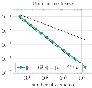
Figure 1. $L^{2}(\Omega)$ errors of the quasi-interpolants $J^{\mathrm{Cl}}_{\mathcal{T}}u$ and $J^{\mathrm{Cl},\boldsymbol{\varphi}}_{\mathcal{T}}u$ for $u(x)=\sin(\pi x)$. The left plot shows the errors where each mesh is a uniform partition of $\Omega=(0,1)$. The right plot shows the errors where two adjacent elements have different mesh-sizes, but each mesh is quasi-uniform, see Section 5.1. Black dotted lines indicate $\mathcal{O}(h)$ and $\mathcal{O}(h^{2})$.

5.2. Mixed method with $H^{-1}(\Omega)$ load

Let $\Omega=(0,1)^{2}$ and consider the manufactured solution

$$u(x,y)=|x-y|^{3/4}\sin(\pi x)\sin(\pi y),\quad(x,y)\in\Omega.$$

This solution has also been considered in [15, Section 5] for the regularized FOSLS. We have that $f=-\Delta u\in H^{-1+1/4-\varepsilon}(\Omega)$ for $\varepsilon>0$. We study the errors of the solutions $(u_{\mathcal{T}},{\boldsymbol{\sigma}}_{\mathcal{T}})$ of the regularized mixed FEM (4) with $Q_{\mathcal{T}}^{\star}=Q^{\mathrm{Cl},\boldsymbol{\varphi}}_{\mathcal{T}}$. Recall that $u_{\mathcal{T}}^{\star}\in\mathcal{P}^{1}(\mathcal{T})$ denotes the postprocessed solution. The errors are displayed in Figure 2. It can be observed that

$$\|u-u_{\mathcal{T}}\|=\mathcal{O}(h),\quad\|{\boldsymbol{\sigma}}-{\boldsymbol{\sigma}}_{\mathcal{T}}\|=\mathcal{O}(h^{1/4}),\quad\|u-u_{\mathcal{T}}^{\star}\|=\mathcal{O}(h^{1+1/4}),$$

in accordance (omitting $\varepsilon$) with the results derived in this work (Corollary 5, Theorem 15, and Corollary 16).

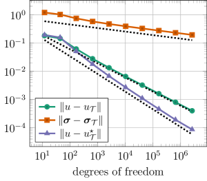
Figure 2. Results for the mixed method for the experiment from Section 5.2. Black dotted lines indicate $\mathcal{O}(h^{1/4})$, $\mathcal{O}(h)$ and $\mathcal{O}(h^{1+1/4})$.

5.3. Postprocessing in the mixed FEM with $L^{2}(\Omega)$ load

We consider the problem setup of [15, Section 6.3], i.e., the manufactured solution

$$u(x,y)=x|x|^{1/2+1/128}(1-x^{2})(1-y^{2}),\quad(x,y)\in\Omega:=(-1,1)^{2}.$$

One verifies that $u\in H^{2}(\Omega)\cap H_{0}^{1}(\Omega)$, thus, $f:=-\Delta u\in L^{2}(\Omega)$ but $f\notin H^{s}(\Omega)$ for $s\geq\tfrac{1}{128}$. In particular, the standard mixed method (2) and the modified mixed method (4) with $Q_{\mathcal{T}}^{\star}=Q^{\mathrm{Cl},\boldsymbol{\varphi}}_{\mathcal{T}}$ are well defined. Table 1 shows a comparison of the errors: For both methods we observe that

$$\|u-u_{\mathcal{T}}\|+\|{\boldsymbol{\sigma}}-{\boldsymbol{\sigma}}_{\mathcal{T}}\|=\mathcal{O}(h),$$

as expected, whereas for the postprocessed solutions we see that

$$\|u-u_{\mathcal{T}}^{\star}\|=\begin{cases}\mathcal{O}(h^{3/2})&\text{for method~{}\eqref{eq:mixed:standard}},\\ \mathcal{O}(h^{2})&\text{for method~{}\eqref{eq:mixed:mod}}.\end{cases}$$

The fact that the postprocessed solution of the modified mixed FEM converges optimally, fits the theory (Theorem 15). We note that, although $f\in L^{2}(\Omega)$ (so that there would be no need to regularize the datum), the regularized method seems to deliver more accurate solutions.

	standard mixed method (2)						regularized mixed method (4)
$\#\mathcal{T}$	$\|{\boldsymbol{\sigma}}-{\boldsymbol{\sigma}}_{\mathcal{T}}\|$	eoc	$\|u-u_{\mathcal{T}}\|$	eoc	$\|u-u_{\mathcal{T}}^{\star}\|$	eoc	$\|{\boldsymbol{\sigma}}-{\boldsymbol{\sigma}}_{\mathcal{T}}\|$	eoc	$\|u-u_{\mathcal{T}}\|$	eoc	$\|u-u_{\mathcal{T}}^{\star}\|$	eoc
4	1.35e+00	—	3.42e-01	—	4.45e-01	—	1.53e+00	—	4.10e-01	—	5.32e-01	—
16	7.95e-01	0.77	1.57e-01	1.12	1.46e-01	1.61	8.04e-01	0.92	1.65e-01	1.31	1.56e-01	1.77
64	4.83e-01	0.72	9.00e-02	0.81	5.41e-02	1.43	4.79e-01	0.75	9.19e-02	0.85	5.72e-02	1.45
256	2.57e-01	0.91	4.79e-02	0.91	1.51e-02	1.84	2.52e-01	0.92	4.81e-02	0.93	1.57e-02	1.87
1024	1.32e-01	0.97	2.43e-02	0.98	4.17e-03	1.86	1.28e-01	0.97	2.43e-02	0.98	4.03e-03	1.96
4096	6.66e-02	0.98	1.22e-02	1.00	1.22e-03	1.77	6.49e-02	0.99	1.22e-02	1.00	1.02e-03	1.98
16384	3.36e-02	0.99	6.10e-03	1.00	3.89e-04	1.65	3.27e-02	0.99	6.10e-03	1.00	2.57e-04	1.99
65536	1.69e-02	0.99	3.05e-03	1.00	1.32e-04	1.56	1.65e-02	0.99	3.05e-03	1.00	6.47e-05	1.99
262144	8.51e-03	0.99	1.52e-03	1.00	4.60e-05	1.52	8.30e-03	0.99	1.52e-03	1.00	1.63e-05	1.99

Table 1. Comparison between the two mixed FEMs for the problem described in Section 5.3.

5.4. Comparison of standard and regularized FOSLS

We consider the Waterfall benchmark problem from [4, Section 5.4] with manufactured solution

$$u(x,y)=x(x-1)y(y-1)e^{-100(x-1/2)^{2}-(y-117)^{2}/10000},\quad(x,y)\in\Omega:=(0,1)^{2}.$$

We note that $f:=-\Delta u\in L^{2}(\Omega)$, and by elliptic regularity (9) we have $u\in H^{2}(\Omega)\cap H_{0}^{1}(\Omega)$. For this experiment we compare the accuracy of the standard FOSLS (3) and the modified FOSLS (5) with $Q_{\mathcal{T}}^{\star}=Q^{\mathrm{Cl},\boldsymbol{\varphi}}_{\mathcal{T}}$. Table 2 shows the errors $\|{\boldsymbol{\sigma}}-{\boldsymbol{\sigma}}_{\mathcal{T}}\|$, $\|u-u_{\mathcal{T}}\|$, and $\|u-u_{\mathcal{T}}\|_{1}$ for both methods. As expected $\|{\boldsymbol{\sigma}}-{\boldsymbol{\sigma}}_{\mathcal{T}}\|$ and $\|u-u_{\mathcal{T}}\|_{1}$ converge at the optimal rate. From Table 2 we even see that the absolute values of $\|{\boldsymbol{\sigma}}-{\boldsymbol{\sigma}}_{\mathcal{T}}\|$ and $\|u-u_{\mathcal{T}}\|_{1}$ for both methods are not distinguishable as $h\to 0$. Only for the $L^{2}(\Omega)$ errors $\|u-u_{\mathcal{T}}\|$ we see a notable difference. Asymptotically, one finds that the $L^{2}(\Omega)$ error in the primal variable for the standard FOSLS is about $42\%$ larger than the $L^{2}(\Omega)$ error for the regularized FOSLS.

	regularized FOSLS (5)						standard FOSLS (3)
$\#\mathcal{T}$	$\|{\boldsymbol{\sigma}}-{\boldsymbol{\sigma}}_{\mathcal{T}}\|$	eoc	$\|u-u_{\mathcal{T}}\|$	eoc	$\|u-u_{\mathcal{T}}\|_{1}$	eoc	$\|{\boldsymbol{\sigma}}-{\boldsymbol{\sigma}}_{\mathcal{T}}\|$	eoc	$\|u-u_{\mathcal{T}}\|$	eoc	$\|u-u_{\mathcal{T}}\|_{1}$	eoc
4	3.37e-02	—	4.43e-03	—	3.41e-02	—	3.79e-02	—	5.11e-03	—	3.64e-02	—
16	4.08e-02	-0.27	4.19e-03	0.08	4.44e-02	-0.38	3.93e-02	-0.05	3.08e-03	0.73	4.23e-02	-0.22
64	2.59e-02	0.65	1.69e-03	1.31	2.84e-02	0.64	2.60e-02	0.60	1.75e-03	0.81	2.96e-02	0.52
256	1.47e-02	0.81	5.37e-04	1.66	1.59e-02	0.84	1.51e-02	0.78	7.22e-04	1.28	1.72e-02	0.78
1024	7.43e-03	0.99	1.85e-04	1.54	1.08e-02	0.56	7.33e-03	1.04	2.41e-04	1.58	1.09e-02	0.66
4096	3.68e-03	1.01	4.56e-05	2.02	5.49e-03	0.98	3.66e-03	1.00	6.32e-05	1.93	5.51e-03	0.99
16384	1.83e-03	1.01	1.13e-05	2.01	2.76e-03	0.99	1.83e-03	1.00	1.60e-05	1.98	2.76e-03	1.00
65536	9.16e-04	1.00	2.82e-06	2.00	1.38e-03	1.00	9.15e-04	1.00	4.01e-06	2.00	1.38e-03	1.00
262144	4.58e-04	1.00	7.05e-07	2.00	6.90e-04	1.00	4.58e-04	1.00	1.00e-06	2.00	6.90e-04	1.00

Table 2. Comparison between the two FOSLS for the problem described in Section 5.4.

References

- [1] F. Bertrand and D. Boffi. First order least-squares formulations for eigenvalue problems. IMA J. Numer. Anal., 42(2):1339–1363, 2022.
- [2] P. B. Bochev and M. D. Gunzburger. Least-squares finite element methods, volume 166 of Applied Mathematical Sciences. Springer, New York, 2009.
- [3] D. Boffi, F. Brezzi, and M. Fortin. Mixed finite element methods and applications, volume 44 of Springer Series in Computational Mathematics. Springer, Heidelberg, 2013.
- [4] P. Bringmann. Computational competition of three adaptive least-squares finite element schemes. arXiv, arXiv:2209.06028, 2022.
- [5] Z. Cai and J. Ku. Optimal error estimate for the div least-squares method with data and application to nonlinear problems. SIAM J. Numer. Anal., 47(6):4098–4111, 2010.
- [6] C. Carstensen. Quasi-interpolation and a posteriori error analysis in finite element methods. M2AN Math. Model. Numer. Anal., 33(6):1187–1202, 1999.
- [7] C. Carstensen. Clément interpolation and its role in adaptive finite element error control. In Partial differential equations and functional analysis, volume 168 of Oper. Theory Adv. Appl., pages 27–43. Birkhäuser, Basel, 2006.
- [8] P. Clément. Approximation by finite element functions using local regularization. Rev. Française Automat. Informat. Recherche Opérationnelle Sér., 9(R-2):77–84, 1975.
- [9] M. Dauge. Elliptic boundary value problems on corner domains, volume 1341 of Lecture Notes in Mathematics. Springer-Verlag, Berlin, 1988. Smoothness and asymptotics of solutions.
- [10] L. Diening, J. Storn, and T. Tscherpel. Interpolation Operator on negative Sobolev Spaces. Math. Comput., in press DOI: 10.1090/mcom/3824 (preprint availabel at https://arxiv.org/abs/2112.08515), 2023.
- [11] A. Ern, T. Gudi, I. Smears, and M. Vohralík. Equivalence of local- and global-best approximations, a simple stable local commuting projector, and optimal approximation estimates in . IMA J. Numer. Anal., 42(2):1023–1049, 2022.
- [12] A. Ern and P. Zanotti. A quasi-optimal variant of the hybrid high-order method for elliptic partial differential equations with loads. IMA J. Numer. Anal., 40(4):2163–2188, 2020.
- [13] T. Führer. Superconvergent DPG methods for second-order elliptic problems. Comput. Methods Appl. Math., 19(3):483–502, 2019.
- [14] T. Führer. Multilevel decompositions and norms for negative order Sobolev spaces. Math. Comp., 91:183–218, 2022.
- [15] T. Führer, N. Heuer, and M. Karkulik. MINRES for second-order PDEs with singular data. SIAM J. Numer. Anal., 60(3):1111–1135, 2022.
- [16] G. N. Gatica. A simple introduction to the mixed finite element method. SpringerBriefs in Mathematics. Springer, Cham, 2014. Theory and applications.
- [17] P. Grisvard. Elliptic problems in nonsmooth domains, volume 24 of Monographs and Studies in Mathematics. Pitman (Advanced Publishing Program), Boston, MA, 1985.
- [18] J. Ku. Sharp -norm error estimates for first-order div least-squares methods. SIAM J. Numer. Anal., 49(2):755–769, 2011.
- [19] F. Millar, I. Muga, S. Rojas, and K. G. Van der Zee. Projection in negative norms and the regularization of rough linear functionals. Numer. Math., 150(4):1087–1121, 2022.
- [20] H. Monsuur, R. Stevenson, and J. Storn. Minimal residual methods in negative or fractional sobolev norms. arXiv, arXiv:2301.10484, 2023.
- [21] I. Muga, S. Rojas, and P. Vega. An adaptive superconvergent finite element method based on local residual minimization. arXiv, arXiv:2210.00390, 2022.
- [22] R. Stenberg. Postprocessing schemes for some mixed finite elements. RAIRO Modél. Math. Anal. Numér., 25(1):151–167, 1991.