Slowly Decaying Ringdown of a Rapidly Spinning Black Hole:
Probing the No-Hair Theorem by Small Mass-Ratio Mergers with LISA

Abstract

The measurability of multiple quasinormal (QN) modes, including overtones and higher harmonics, with the Laser Interferometer Space Antenna is investigated by computing the gravitational wave (GW) signal induced by an intermediate or extreme mass ratio merger involving a supermassive black hole (SMBH). We confirm that the ringdown of rapidly spinning black holes are long-lived, and higher harmonics of the ringdown are significantly excited for mergers of small mass ratios. We investigate the measurability and separability of the QN modes for such mergers and demonstrate that the observation of GWs from rapidly rotating SMBHs has an advantage for detecting superposed QN modes and testing the no-hair theorem of black holes.

I Introduction

We are in a golden age of gravitational-wave (GW) astronomy, where mergers of binary black holes (BHs) are discovered by GW interferometers Abbott et al. (2016a, 2019a, 2021a, 2021b, 2021c); Nitz et al. (2021); Olsen et al. (2022). The end product of a merger is a distorted single BH, which settles down to a Kerr BH by radiating GWs. This ringdown phase is characterized by a set of damped sinusoids called quasinormal (QN) modes, and is an important probe to test general relativity in the strong-gravity regime Kokkotas and Schmidt (1999); Nollert (1999); Berti et al. (2009). QN modes from BH merger remnants have been detected for a large number of events, and were used for various tests of general relativity (e.g., Abbott et al. (2016b, 2019b, 2021d, 2021e)).

QN modes consist of fundamental modes and overtones, where the latter is short-lived but can be important for characterizing the ringdown signal Giesler et al. (2019); Oshita (2021). Detection of overtones from ringdowns is important for e.g. tests of the no-hair theorem (Dreyer et al., 2004). Evidence of an overtone was claimed in the ringdown of GW 150914 Isi et al. (2019), although its significance is still controversial Cotesta et al. (2022); Finch and Moore (2022); Isi and Farr (2022).

A key parameter that governs the relative strength between fundamental modes and overtones is the spin parameter, $j\equiv J/M^{2}$, of the remnant BH. $J$ is the angular momentum and $M$ is the mass of the BH. Recently one of the authors found Oshita (2021, 2023) that remnants with rapid spin ($j\gtrsim 0.9$) can have a ringdown dominated by higher overtones and higher angular modes. The more QN modes are detected, the more accurate the test of general relativity would be. Therefore GW ringdown of a highly spinning or near-extremal BH may be a preferred signal to test general relativity. However the final spin of observed BH mergers is typically $\approx 0.7$ (Abbott et al., 2019a, 2021a, 2021c), and such extreme spins may be difficult to probe for mergers of stellar-mass BHs whose natal spins are expected to be rather low (Fuller and Ma, 2019).

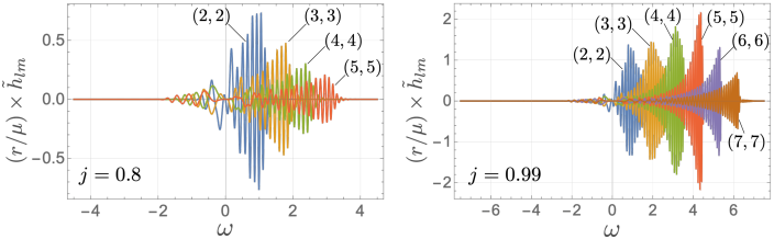
Figure 1: Spectra of the GW signal induced by a compact object plunging into a BH with $L_{z}=1$ and two BH spins, $j=0.8$ (left) and $0.99$ (right). We adopt the normalization $2M=1$.

In this work we consider the possibility of exploring overtones and higher angular modes of rapidly spinning BHs with intermediate/extreme mass ratio mergers involving a supermassive BH (SMBH). These sources, especially with SMBHs in the mass range $10^{6}$–$10^{7}\ M_{\odot}$, are targets for space-based GW detectors like the Laser Interferometer Space Antenna (LISA) Amaro-Seoane et al. (2017, 2022). Notably these SMBHs are predicted to have large spins due to gas accretion upon their growth (Dotti et al. (2013); Dubois et al. (2014); Bustamante and Springel (2019), but see Barausse (2012)). Although systematic uncertainties may exist in the fitting, X-ray spectra of local SMBHs in this mass range indicate high spins of $>0.9$, consistent with this scenario (Reynolds, 2013; Vasudevan et al., 2016; Reynolds, 2021).

Using the waveform modeling of a particle plunging into a rapidly spinning BH and extracting the excited QN modes with a fitting analysis, we estimate the measurability of multiple QN modes, including higher overtones and higher angular modes, by LISA. We find that these modes can be detectable out to cosmological distances, realizing a novel probe of gravity in the near-extreme Kerr spacetime. We also evaluate the error of the measurability and separability of the QN modes Ota and Chirenti (2022); Bhagwat et al. (2022) to assess the feasibility of measuring individual modes.

II ringdown for a small mass ratio merger

In this work we focus on simulating a merger of small mass ratio, such that its dynamics can be well approximated by a test particle plunging into a SMBH. We numerically compute the GW signal induced by a particle plunging into a rotating hole using the Sasaki-Nakamura (SN) equation Sasaki and Nakamura (1982):

$$\left(\frac{d^{2}}{dr^{\ast}{}^{2}}-F_{lm}\frac{d}{dr^{\ast}}-U_{lm}\right)X_{lm}=\tilde{T}_{lm},$$ (1)

where $X_{lm}$ is a perturbation variable of the gravitational field, $r^{\ast}$ is the tortoise coordinate, $F_{lm}$ and $U_{lm}$ are functions with explicit form given in Ref. Sasaki and Nakamura (1982), and $\tilde{T}_{lm}$ is the source term associated with the plunging particle. The form of $\tilde{T}_{lm}$ is given in Ref. Kojima and Nakamura (1984) and can be obtained from the geodesic motion of the object. The orbital angular momentum of the plunging orbit is $\mu\times L_{z}$, and the infalling condition is $-2M(1+\sqrt{1+j})<L_{z}<2M(1+\sqrt{1-j})$. We here assume that the value of $L_{z}$ for infalling objects is typically ${\cal O}(M)$ and take $L_{z}=2M$ throughout the manuscript. Integers $l$ and $m$ are, respectively, the angular and azimuthal numbers of the spheroidal harmonics. We here consider a situation where the trajectory of a compact object of mass $\mu$ is restricted to the equatorial plane ($\theta=\pi/2$) and the total energy of the object (including rest energy) is $\mu$. The self-force of the object can be neglected, which is valid for a small mass ratio $q\equiv\mu/M\ll 1$. Using the Green’s function technique, one can solve the SN equation as

$$\begin{split}\lim_{r^{\ast}\to\infty}X_{lm}(\omega,r^{\ast})&=X_{lm}^{\rm(out)}(\omega)e^{i\omega r^{\ast}}\\ &=\int dr^{\prime}\tilde{T}_{lm}(r^{\prime},\omega)G(r^{\prime},r^{\ast},\omega),\end{split}$$ (2)

where $G(r^{\prime},r^{\ast},\omega)$ is the Green’s function that is obtained from the homogeneous solution of the SN equation. We then obtain the GW spectrum

$$\tilde{h}=\sum_{l,m}\tilde{h}_{lm}(\omega)=\sum_{l,m}-\frac{2}{\omega^{2}}{}_{-2}S_{lm}(a\omega,\pi/2)R_{lm}(\omega),$$ (3)

where $a\equiv J/M$ and ${}_{-2}S_{lm}$ is the spin-weighted spheroidal harmonics, assuming an edge-on observer with argument $\pi/2$. The time-domain data $h=h_{+}+ih_{\times}=\sum_{(l,m)}h_{lm}$ is obtained by the inverse Laplace transformation of $\tilde{h}$. The function $R_{lm}(\omega)$ is obtained by properly normalizing $X_{lm}$, and its explicit form is provided in Ref. Sasaki and Nakamura (1982).

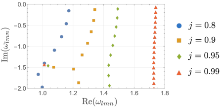
Figure 2: Kerr QN frequencies for $(l,m)=(2,2)$, with the normalization $2M=1$. Different markers correspond to different BH spins, and $n$ increases from top to bottom of this plot. For a higher spin, an increasing number of overtones have small Im$(\omega_{lmn})$ and are long-lived.

The GW spectra computed with this scheme is shown in Figure 1. One can see that $(l,m)=(2,2)$ dominates the GW signal for an intermediate spin ($j=0.8$ in Figure 1), but higher angular modes are significantly excited for a near-extremal Kerr BH of $j=0.99$. We are interested in the signal induced by a compact object plunging into a rapidly spinning BH, as more QN modes are long-lived for higher spins (Figure 2).

In the next section, we show that a number of highly damped modes dominate the early ringdown of a near-extremal BH by fitting multiple overtones and fundamental modes to the GW signal. Then we show that rapidly spinning BHs are better targets to perform a high-precision detection of multiple QN modes, including higher angular modes and higher overtones.

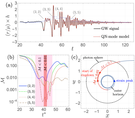
Figure 3: Expected GW signal induced by the compact object plunging into a SMBH with $j=0.99$. (a) Time-domain waveform of the GW signal $h_{\times}(t)$ (black solid) and the QN-mode model obtained by the fitting analysis, with $t^{\ast}=42$ and $n_{\rm max}=20$ for each angular mode in $2\leq l=m\leq 5$ (red dashed). The blue dotted lines are $|h_{lm}|$ for each angular mode included in our analysis. (b) Mismatch ${\cal M}$ with respect to $t^{\ast}$ for $(l,m)=(2,2)$, $(3,3)$, $(4,4)$, and $(5,5)$. All angular modes we computed satisfy ${\cal M}<0.01$ in the range $40\lesssim t^{\ast}\lesssim 43$. (c) Trajectory of the compact object plunging into the BH. The red and pink lines on the trajectory correspond to the shaded regions in (b) with red (${\cal M}<0.01$) and pink (${\cal M}<0.1$), respectively. The blue triangle indicates the position at which the particle sources the signal peak.

III Excitation of overtones

The measurability of the QN modes is highly sensitive to the start time of ringdown $t^{\ast}$ because (i) it is a superposition of QN modes, each of which is exponentially damped in time, and (ii) overtones may dominate the signal at early times. The exact start time of the ringdown is unknown, but one can obtain a best fit value by fitting multiple QN modes to the GW signal. We then show that the ringdown starts earlier than the strain peak, around the time when the object plunges into the photon sphere.

We perform fitting analysis of QN modes with a complex frequency $\omega_{lmn}$ including overtones of $n\leq n_{\rm max}$ and angular modes of $2\leq l=m\leq 5$. The fitting is done in the frequency domain by using the QN mode model

$$\tilde{h}_{lm}=\sum_{n}^{n_{\rm max}}\frac{A_{lmn}}{\omega-\omega_{lmn}}e^{i\omega_{lmn}t^{\ast}+i\phi_{lmn}},$$ (4)

to avoid the instability at early ringdown Oshita (2023) and to treat $t^{\ast}$ as one of the fitting parameters Finch and Moore (2021). In equation (4), $A_{lmn}$ and $\phi_{lmn}$ are fitting parameters associated with the amplitude and phase of a QN mode with $\omega=\omega_{lmn}$, respectively. Figure 3(a) shows that the best fit value of $t^{\ast}$ (in units of $2M$) is in the range $40\lesssim t^{\ast}\lesssim 43$, where the mismatch ${\cal M}$ is less than $0.01$. The range of $t^{\ast}$ with ${\cal M}<0.1$ corresponds to the moments after the particle plunges into the photon sphere [see Figure 3(b)]. This is consistent with the fact that GW ringdown is a signal associated with the photon sphere Ferrari and Mashhoon (1984). We also find that including up to higher overtones ($n_{\rm max}\gtrsim 15$) in the fit is necessary to guarantee the convergence of the mismatch (Figure 4). That is, once we admit the start time of ringdown is soon after the compact object plunges into the photon sphere ($t^{\ast}\sim 42$ in our setup), not only the fundamental modes with quadrupole moment but also a number of long-lived modes and higher harmonics are significantly excited for a near-extremal BH. It has an advantage for measuring multiple QN modes, including overtones and higher harmonics, and for accurately testing general relativity. Indeed, it is reported that a fraction of SMBHs can have near-extremal spin parameters of $j\gtrsim 0.99$ Reynolds (2013); Vasudevan et al. (2016); Reynolds (2021). In the following, we show such SMBHs are suitable observation targets to detect multiple QN modes.

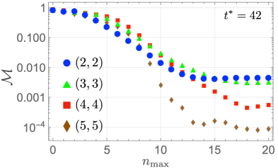
Figure 4: Mismatch of the fit of QN modes to the GW data for $j=0.99$. The fitting is performed for $l=m=2$, $3$, $4$, and $5$.

IV No-hair test of SMBHs with LISA

IV.1 Measurability of superposed QN modes

Let us evaluate the measurability of multiple QN modes of rotating BHs, and its feasibility for tests of the no-hair theorem.

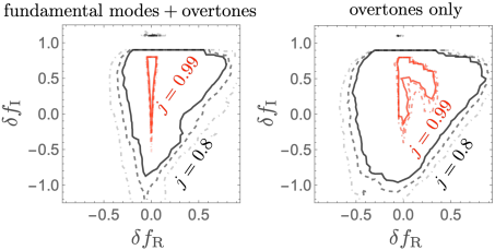
Figure 5: Precision for measuring deviations of multiple QN modes from general relativity, for (left) $H_{\delta}^{\rm(F+O)}$ model with $(D_{\rm L},\tilde{M},q)=(3\ \text{Gpc},10^{7}M_{\odot},10^{-3})$ and (right) $H_{\delta}^{\rm(O)}$ model with $(1\ \text{Gpc},10^{7}M_{\odot},10^{-3})$. Red and black colors show spins of $j=0.99$ and $0.8$ respectively. Outside the solid, dashed and dot-dashed contours, the likelihood ratio ${\cal L}$ takes values of $>3.2$, $>10$, and $>100$, respectively. As higher overtones can be important for higher angular modes (see Figure 4 and cf. Ref. Mourier et al. (2021)), we include many overtones to model the waveforms. For $j=0.99$, we include QN modes up to $n=21$ for each mode $l=m=2$, $3$, $4$, and $5$. For $j=0.8$, on the other hand, QN modes up to $n=16$ are included for each mode $l=m=2$, $3$ and $4$.

We here consider detections of them with LISA, which is sensitive to signals of $\sim 0.01$ Hz and is suitable for detecting ringdown of SMBHs with mass $\sim 10^{6}$–$10^{7}M_{\odot}$. The sensitivity curve can be modeled by an analytic function $\tilde{S}_{n}(f)$ Robson et al. (2019):

$$\tilde{S}_{n} =\frac{1}{{\cal F}}\left(\frac{P_{\rm OMS}}{L^{2}}+(1+\cos^{2}(f/f_{\ast}))\frac{2P_{\rm acc}}{(2\pi f)^{4}L^{2}}\right),$$ (5)

$${\cal F} \equiv\frac{3}{10}\left(1+0.6\times(f/f_{\ast})^{2}\right)^{-1},$$ (6)

where $2L$ is the round-trip light travel distance, $f_{\ast}\equiv c/(2\pi L)$ is the transfer frequency, $P_{\rm OMS}$ and $P_{\rm acc}$ are the single-link optical metrology noise and the single test mass acceleration noise, respectively. The function ${\cal F}$ is the sky/polarization average of the antenna pattern functions. We include the galactic confusion noise from compact binaries,

$$S_{c}(f)=Af^{-7/3}e^{-f^{\alpha}+\beta f\sin{(\kappa f)}}[1+\tanh(\gamma(f_{k}-f))]\text{Hz}^{-1},$$ (7)

where $A=9\times 10^{-45}$ and the parameter set $\{\alpha,\beta,\gamma,\kappa,f_{k}\}$ is fixed with the values for a four-year mission (we use Table 1 in Ref. Robson et al. (2019)). Then we obtain the full sensitivity curve as $S_{n}(f)=\tilde{S}_{n}(f)+S_{c}(f)$. Using $S_{n}$, we evaluate the SNR of the GW signal and the likelihood ratio, to investigate the support for the model of the no-hair QN modes $H_{0}$ over a modified model $H_{\delta}$ consisting of a set of complex frequencies deviated from the no-hair values.

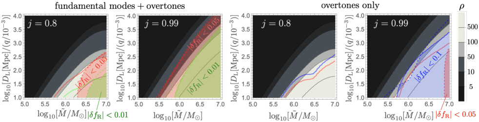
Figure 6: Distances out to which tests with multiple QN modes are possible. The contours show the SNR of the ringdown, as a function of the redshifted SMBH mass $\tilde{M}$ and the luminosity distance $D_{\rm L}$ with mass ratio $q$ scaled as $10^{-3}$. The solid and dashed lines indicate $\delta f_{\rm R}>0$ and $\delta f_{\rm R}<0$, respectively. In the shaded regions, below both the solid and dashed lines, one can measure the real part of QN frequencies with (green) $\lesssim 1\%$, (red) $\lesssim 5\%$, and (blue) $\lesssim 10\%$, respectively. We here set $\delta f_{\rm I}=0$, as observations are rather insensitive to $\delta f_{\rm I}$ (see Figure 5).

For the modification of the no-hair model, we consider two types of modifications: (i) a model $H_{\delta}^{\rm(F+O)}$ for which all QN frequencies, including fundamental modes and overtones, are modified as

$$\omega_{lmn}=\text{Re}(\omega_{lmn}^{\rm(GR)})(1+\delta f_{\rm R})+i\text{Im}(\omega_{lmn}^{\rm(GR)})(1+\delta f_{\rm I}),$$ (8)

where $\omega_{lmn}^{\rm(GR)}$ are the QN frequencies in general relativity, and (ii) a model $H_{\delta}^{\rm(O)}$ for which only overtones are modified with the above expressions. Depending on the parameters of the remnant mass and spin, the whole QN mode frequencies coherently change like the model $H_{\delta}^{\rm(F+O)}$. As such, we can estimate the feasibility of the test of the no-hair theorem, which states that the frequency and decay rate of QN modes are uniquely set by the remnant mass and spin. On the other hand, comparing the likelihood ratio with $H_{\delta}^{\rm(F+O)}$ and the one with $H_{\delta}^{\rm(O)}$, we can see the efficiency of the inclusion of overtones in the test of the no-hair theorem. The models $H_{0}$, $H_{\delta}$ are respectively given by the superposition of GR or modified QN modes, and the model parameters, i.e., an amplitude and phase, are assigned to each QN mode. The best fit values of the amplitudes and phases are determined by the Mathematica function “Fit”. Our artificial modification to QN modes affects the model parameters and the likelihood ratio. The SNR $\rho$ and the likelihood ratio ${\cal L}$ are Cabero et al. (2020)

$$\rho =\sqrt{\braket{\tilde{h}_{+},\tilde{h}_{+}}+\braket{\tilde{h}_{\times},\tilde{h}_{\times}}},$$ (9)

$${\cal L} =\frac{p(\tilde{h}_{+}|H_{0})}{p(\tilde{h}_{+}|H_{\delta})}\frac{p(\tilde{h}_{\times}|H_{0})}{p(\tilde{h}_{\times}|H_{\delta})},$$ (10)

where $H_{\delta}$ is $H_{\delta}^{\rm(F+O)}$ or $H_{\delta}^{\rm(O)}$,

$$\braket{x,y}\equiv 4\text{Re}\int^{\infty}_{0}\frac{x(f)y^{\ast}(f)}{S_{n}}df,$$ (11)

$\tilde{h}_{+/\times}(f)$ is the Fourier transform of $h_{+/\times}(t)$, and $p(d|H)$ is the likelihood

$$p(d|H(\vec{\vartheta}))\propto\exp\left[-\frac{1}{2}\braket{d-H(\vec{\vartheta}),d-H(\vec{\vartheta})}\right],$$ (12)

with a given data, $d$, and a model function, $H(\vec{\vartheta})$, for a set of the fitting parameters $\vec{\vartheta}$, i.e., the amplitude and phase of each QN mode and $t^{\ast}$.

Figure 5 shows the precision of constraining deviations of multiple QN modes for different thresholds of ${\cal L}$. We find that no-hair tests of rapidly rotating BHs are more powerful than those with BHs of intermediate spin. For the $H_{\delta}^{\rm(F+O)}$ model in the left panel, the measurement error of the real frequency is $\lesssim 80\%$ for $j=0.8$, but only $\lesssim 10\%$ for $j=0.99$. We here take $(D_{\rm L},\tilde{M},q)=(3~{}\text{Gpc},10^{7}M_{\odot},10^{-3})$, where $D_{\rm L}$ is the luminosity distance and $\tilde{M}=(1+z)M$ is the redshifted mass of a SMBH that includes the effect of redshift $z$.

Overtones more quickly damp with time, and hence measuring deviations of overtones is likely more challenging. Nevertheless, for near-extremal BHs, the damping is very weak and even overtones may be measured with good precision. The right panel in Figure 5 shows the high feasibility of measuring overtones for a rapidly spinning BH. We here assume $(D_{\rm L},\tilde{M},q)=(1~{}\text{Gpc},10^{7}M_{\odot},10^{-3})$. In both models that we considered, the uncertainty in the damping rate $\delta f_{\rm I}$ of QN modes is larger. This would be caused by the dispersive distribution of QN mode frequencies towards the imaginary axis in the complex frequency plane (see Figure 2). That is, the fundamental mode and overtones have close values of the real part of QN mode frequencies whereas they have dispersive values in the imaginary part. This may cause the large uncertainty in $\delta f_{I}$ as shown in Figure 5. A similar conclusion and a large uncertainty in the imaginary part was reported in Isi et al. (2019), where the no-hair test was performed for GW150914 Abbott et al. (2016c).

Figure 6 summarizes the expected distance out to which we can measure multiple QN modes with high precision. In this section we discuss the prospects for LISA, for moderate and extreme mass ratios.

For moderate mass ratios of $q\sim 10^{-3}$, it corresponds to a merger between a SMBH and an intermediate-mass BH (IMBH). A scenario usually considered for such mergers is clusters hosting IMBHs falling into the galactic nuclei (Miller, 2004; Portegies Zwart et al., 2006; Matsubayashi et al., 2007; Arca-Sedda and Capuzzo-Dolcetta, 2019; Arca-Sedda and Gualandris, 2018). The event rate is uncertain, but recent N-body simulations find a range $0.003$–$0.03$ Gpc^-3 yr^-1 Arca-Sedda and Capuzzo-Dolcetta (2019); Arca-Sedda and Gualandris (2018), or $2$–$20$ yr^-1 within $z<1$ ($D_{\rm L}\lesssim 7$ Gpc) Amaro-Seoane et al. (2022). For the $H_{\delta}^{\rm(F+O)}$ model with $j=0.99$ multiple QN frequencies can be measured within $\sim 5\%$ ($\sim 1\%$) for sources at $D_{\rm L}\lesssim 10$ Gpc ($\lesssim 3$ Gpc), and thus no-hair tests of SMBHs are promising. For the $H_{\delta}^{\rm(O)}$ model, one may constrain the real frequencies within $\lesssim 10\%$ for sources out to a few Gpc, corresponding to an event rate of $0.1$–$1$ yr^-1.

The likelihood ratio for the model of $H_{\delta}^{\rm(O)}$ with $\delta f_{\rm R}>0$ is more significant than that with $\delta f_{\rm R}<0$ (see Figure 6). Being sensitive to the modification of $\delta f_{\rm R}>0$ is reasonable since the higher-frequency modes of $\omega\gtrsim\omega_{lmn}$ in the GW signal are exponentially suppressed (see Ref. Oshita (2023) for more details).

For extreme mass ratios of $q<10^{-5}$, it corresponds to a stellar-mass BH plunging into a SMBH. Such plunges are expected not to be strong GW emitters, as we also deduce from Figure 6. The EMRI rate for a Milky-Way like Galaxy is estimated to be $10^{-6}$–$10^{-5}$ yr^-1, i.e. an event rate of $10^{-8}$–$10^{-7}$ Mpc^-3 yr^-1 (Amaro-Seoane (2018) and references therein). Plunge orbits can be up to $100$ times more likely than EMRIs Bar-Or and Alexander (2016); Babak et al. (2017), so we expect plunges of $\sim 10\ M_{\odot}$ BHs within the detectable distance ($\lesssim 10$ Mpc) at a rate of $<0.1$ yr^-1. Recently a new formation channel of IMBHs in galactic nuclei was proposed, where stellar-mass BHs grow in situ up to $\sim 10^{4}\ M_{\odot}$ by collisions with surrounding stars (Rose et al., 2022). If such growth is efficient, this would likely enhance the above rates.

IV.2 Separability and measurability of individual QN modes

In the previous section, we studied the measurability of superposed QN modes, where we required that the SNR for the secondary QN mode is above a given detectability threshold. However, to assess LISA’s potential for no-hair tests with ringdown signals, it also is important to evaluate the separability and measurability of individual QN modes (BH spectroscopy).

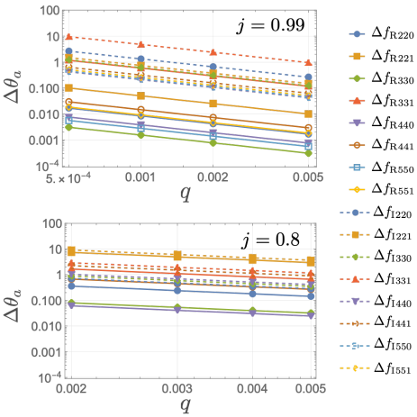
Figure 7: The measurability of the real (solid) and imaginary (dashed) parts of the QN modes for a near-extremal $(j=0.99)$ and medium spin $(j=0.8)$ are shown with respect to the mass ratio $q$. The luminosity distance and the mass of the SMBHs are set to $D_{\rm L}=1$ Gpc and $M=10^{7}M_{\odot}$, respectively.

Let us evaluate the measurability and separability of the fundamental QN mode and the first overtone to see the feasibility of the BH spectroscopy Ota and Chirenti (2022); Bhagwat et al. (2022). The statistical errors on a model parameter $\theta_{a}$ are given by

$$\sigma_{\theta_{a}}=\sqrt{(\Gamma^{-1})^{aa}}$$ (13)

where $\Gamma^{-1}$ is the inverse of the Fisher matrix,

$$\Gamma_{ab}=\left\langle\frac{\partial\tilde{h}}{\partial\theta_{a}},\frac{\partial\tilde{h}}{\partial\theta_{b}}\right\rangle,$$ (14)

with $\braket{x,y}$ defined as in equation (11). We here compute the Fisher matrix with the following parameter set

$$\theta_{a}=\bigcup_{lmn}\{f_{\rm R}{}_{lmn},f_{\rm I}{}_{lmn},A_{lmn},\phi_{lmn}\},$$ (15)

where the parameter set has the fundamental mode ($n=0$) and the first overtone $(n=1)$. The angular modes in the parameter set are $(l,m)=(2,2)$, $(3,3)$, $(4,4)$, $(5,5)$ for $j=0.99$. For $j=0.8$, it has $(l,m)=(2,2)$, $(3,3)$, $(4,4)$. We use the waveform we numerically obtained in Sec. II and use a Mathematica function “Fit” to obtain the best fit model of (4). We then compute the Fisher matrix (14) by analytically computing the derivative of (4) and estimate the statistical errors from the inverse matrix $(\Gamma^{-1})_{ab}$. From the statistical errors, we can evaluate the separability based on the Rayleigh criterion Ota and Chirenti (2022); Bhagwat et al. (2022):

$$s[\theta_{a},\theta_{b}]\equiv\text{max}[\sigma_{a},\sigma_{b}]/|\hat{\theta}_{a}-\hat{\theta}_{b}|<1,$$ (16)

where $\hat{\theta}_{a}$ is the true value of $\theta_{a}$. Also, we can estimate the measurability (i.e. measurement error) with Bhagwat et al. (2022)

$$\Delta\theta_{a}=\sigma_{\theta_{a}}/\hat{\theta}_{a}.$$ (17)

The signal has $x\%$ measurability if the set of $\{\Delta\theta_{a}\}$ satisfies

$$\max_{i}[\Delta\theta_{i}]<\frac{x}{100}.$$ (18)

From this quantity, we can also examine the hierarchy of measurability among the modes we are interested in.

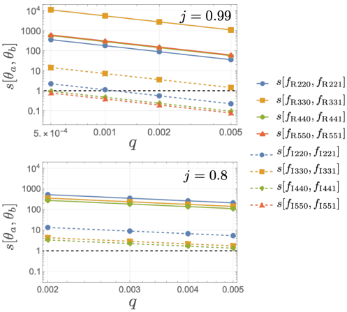
Figure 8: The separability of the real (solid) and imaginary parts of the QN modes for a near-extremal $(j=0.99)$ and medium spin $(j=0.8)$ are shown with respect to the mass ratio $q$. The luminosity distance and the mass of the SMBHs are set to $D_{\rm L}=1$ Gpc and $M=10^{7}M_{\odot}$, respectively. The black dashed line, below which $s[\theta_{a},\theta_{b}]<1$, shows the threshold of the separability of $\theta_{a}$ and $\theta_{b}$.

Figures 7 and 8 show the value of $\Delta{\theta}_{a}$ and $s[\theta_{a},\theta_{b}]$, respectively. We can read that the errors in the measurability and that in the separability for $j=0.99$ are generally smaller than those for $j=0.8$ at the same luminosity distance $D_{\rm L}$, remnant mass $M$, and the mass ratio of $q\leq 0.005$. The real parts of the QN mode frequencies for $j=0.8$ all have larger measurement errors. In the case of $j=0.99$, the error of the real part of the QN frequencies with $n=0$ and $(l,m)=(4,4)$ and $(5,5)$ take the smallest values (i.e., highest precision) among them. The real part of QN frequencies of the first overtones can be still measurable in the level of $\Delta f_{{\rm R}{lm1}}\lesssim 0.01$. On the other hand, the imaginary parts of the QN frequencies for higher harmonics are measurable with $\Delta f_{{\rm I}{lm1}}\sim 0.1$. The error of the imaginary part of QN frequencies in the separability is smaller and can be resolvable for the modes of higher harmonics (see Figure 8). On the other hand, the real parts of QN frequencies for $n=0$ and $n=1$ are too close to resolve especially for $j\sim 0.99$ (see Figures 2 and 8). The QN modes for $j=0.8$ are difficult to distinguish each other in our setup as the damping rates in QN modes are larger.

In a previous work Bhagwat et al. (2022), such measurement errors by LISA were computed for mergers of nonspinning BHs with mass ratio of $0.1\lesssim q\leq 1$ and total mass of $10^{6}M_{\odot}$. While varying $q$ just changes the overall scale of the measurement error, varying the remnant mass and spin may change even the hierarchy among different modes. Indeed, our result shows that the higher angular modes, i.e., $(4,4,0)$ and $(5,5,0)$, have the first three smallest measurement errors for $j=0.99$ whereas $(2,2,0)$ mode takes the smallest error for the case considered by Bhagwat et al. (2022) (their Figure 4). As the higher angular modes may dominate the ringdown signal for a rapidly spinning BH as shown in Figure 1, the rapid spin of the remnant BH may affect the hierarchy.

V Conclusion

In this paper, we studied the measurability and separability of multiple QN modes emitted by near extremal SMBHs, which may exist at the center of galaxies according to the X-ray observation of the accretion disks Dotti et al. (2013); Dubois et al. (2014); Bustamante and Springel (2019). The measurability of superposed QN modes is estimated by the SNR of a ringdown signal that is obtained by the fit of QN modes to the whole GW data (Figure 6). The goodness of the fit with the GR QN modes was assessed by the likelihood ratio (Figures 5 and 6). To assess the ability of the BH spectroscopy, we computed the statistical error to obtain the errors in the separability (16) and in the measurability (17). We then found that the separability and measurability for mergers involving near-extremal SMBHs of $j=0.99$ are generally better than those with SMBHs of moderate spins of $j=0.8$ (Figures 7 and 8). The measurement error of the real part of QN frequencies can be $\lesssim 1\%$ and the separability condition is satisfied for the imaginary part when $D_{\rm L}\lesssim 1$ Gpc and $q\sim 0.005$. We thus conclude that intermediate (and possibly extreme) mass ratio mergers can be unique targets for LISA to probe multiple QN modes of rapidly spinning BHs, and an important target for tests of gravity in a near-extreme Kerr spacetime.