Efficient Selection of Informative Alternative Relational Query Plans for Database Education

Abstract

Given an sql query, a relational query engine selects a query execution plan (qep) for processing it. Off-the-shelf rdbms typically only expose the selected qep to users without revealing information about representative alternative query plans (aqp) considered during qep selection in a user-friendly manner. Easy access to representative aqps is useful in several applications such as database education where it can facilitate learners to comprehend the qep selection process during query optimization. In this paper, we present a novel end-to-end and generic framework called arena that facilitates exploration of informative alternative query plans of a given sql query to aid the comprehension of qep selection. Under the hood, arena addresses a novel problem called informative plan selection problem (tips) which aims to discover a set of $k$ alternative plans from the underlying plan space so that the plan interestingness of the set is maximized. Specifically, we explore two variants of the problem, namely batch tips and incremental tips, to cater to diverse set of users. Due to the computational hardness of the problem, we present a 2-approximation algorithm to address it efficiently. Exhaustive experimental study demonstrates the superiority of arena to several baseline approaches. As a representative use case of arena, we demonstrate its effectiveness in supplementing database education through a user study and academic assessment involving real-world learners.

I Introduction

A relational query engine selects a query execution plan (qep), which represents an execution strategy of an sql query, from many alternative query plans (aqps) by comparing their estimated costs. Major off-the-shelf relational database systems (rdbms) typically only expose the qep to an end user. They do not reveal a representative set of aqps considered by the underlying query optimizer during the selection of a qep in a user-friendly manner. Although an rdbms (e.g., PostgreSQL) may allow one to manually pose sql queries with various constraints on configuration parameters to view the corresponding qeps containing specific physical operators (e.g., SET enable_hashjoin = true), such strategy demands not only familiarity of the syntax and semantics of configuration parameters, but also a clear idea of the AQPs that one is interested. This is often impractical to assume (e.g., in education environment where many learners are taking the database systems course for the first time). Consider the following motivating scenario.

Example I.1

Lena is currently enrolled in an undergraduate database systems course. She wishes to explore some of the representative aqps for the following query from the TPC-H benchmark after viewing its qep as depicted in Fig. 1(a).

⬇

SELECT s_acctbal, s_name, n_name, s_address, s_phone

FROM supplier, nation, region

WHERE s_acctbal>=5000 and s_nationkey = n_nationkey and n_regionkey = r_regionkey;

Specifically, Lena is curious to know whether there are aqps that have similar (resp. different) structure and physical operators but very different (resp. similar) estimated cost? If there are, then how they look like? Examples of such aqps are shown in Fig. 1(b)-(d).    

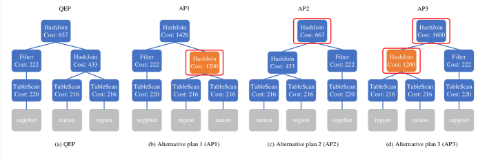
Figure 1: Example of qep and alternative query plans (aqps).

Clearly, a user-friendly tool that can facilitate retrieval and exploration of “informative” aqps associated with a given query can greatly aid in answering Lena’s questions. Unfortunately, very scant attention has been given to build such tools by the academic and industrial communities. Recent efforts for technological support to augment learning of relational query processing primarily focused on the natural language descriptions of qeps [29; 44] and visualization of the plan space [17]. In this paper, we present an end-to-end framework called arena (AlteRnative quEry plaN ExplorAtion) to address this challenge. Our approach not only has positive feedback from learners (Section VIII-A) but, more importantly, eventually improves academic outcomes (Section VIII-B).

Selecting a set of representative aqps is a technically challenging problem. Firstly, the plan space can be prohibitively large [7]. Importantly, not all aqps potentially support understanding of the qep selection process. Hence, it is ineffective to expose all plans. Instead, it is paramount to select those that are informative. However, how do we quantify informativeness in order to select plans? For instance, in Fig. 1(b)-(d), which plans should be revealed to Lena? Certainly, any informativeness measure needs to consider the plans (including the qep) that an individual has already viewed for her query so that highly similar plans are not exposed to them. It should also be cognizant of individuals’ interests in this context. Secondly, it can be prohibitively expensive to scan all aqps to select informative ones. How can we design efficient techniques to select informative plans? Importantly, this cannot be integrated into the enumeration step of the query optimizer as informative aqps need to be selected based on the qep an individual has seen.

Thirdly, at first glance, it may seem that we can select $k>1$ alternative query plans where $k$ is a value specified by a user. Although this is a realistic assumption for many top-$k$ problems, our engagement with users reveal that they may not necessarily be confident to specify the value of $k$ always (detailed in Section VIII-A). One may prefer to iteratively view one plan-at-a-time and only cease exploration once they are satisfied with the understanding of the alternative plan choices made by the optimizer for a specific query. Hence, $k$ may not only be unknown apriori but also the selection of an aqp at each iteration to enhance their understanding of different plan choices depends on the plans viewed by them thus far. This demands for a flexible solution framework that can select alternative query plans in the absence or presence of $k$ value. Lastly, any proposed solution should be generic so that it can be easily realized on top of majority of existing off-the-shelf rdbms.

In this paper, we formalize the aforementioned challenges into a novel problem called informative plan selection (tips) problem and present arena to address it. Specifically, given an sql query and $k\geq 1$ (when $k$ is unspecified it is set to 1), it retrieves $k$ alternative query plans (aqps) that maximize plan informativeness. Such query plans are referred to as informative query plans. To this end, we introduce two variants of tips, namely batch tips (b-tips) and incremental tips (i-tips), to cater for scenarios where $k$ is specified or unspecified by a user, respectively. We introduce a novel concept called plan informativeness to capture the aforementioned challenges associated with the selection of informative aqps. Specifically, it embodies the preferences of real-world users (based on their feedback) by mapping them to distance (computed by exploiting differences between plans w.r.t. structure, content and estimated cost) and relevance of alternative plans with respect to the qep or the set of alternative plans viewed by a user thus far. Next, given the computational hardness of the tips problem, we present a 2-approximation algorithm to address both the variants of the problem efficiently. Specifically, it has a linear time complexity w.r.t. the number of candidate aqps. Given that the number of such candidates can be very large for some queries. we propose two pruning strategies to prune them efficiently. We adopt orca [40] to retrieve the candidate plan space for a given sql query in arena as it enables us to build a generic framework that can easily be realized on majority of existing rdbms.

Lastly, we demonstrate the usefulness of arena by deploying it in the database systems course at Xidian University. Specifically, we analyze the feedback from real-world learners and their academic performance w.r.t. the understanding of the qep selection process. Our analysis reveals the efficiency and effectiveness of our solutions to help learners understand alternative query plans in the context of QEP selection.

In summary, this paper makes the following key contributions.

• We adopt a learner-centered approach to characterize the notion of informative query plans for database education by engaging real-world learners (Section II), and present the notion of plan informativeness (Section IV) to quantitatively model the informativeness of aqps.

• We present a novel informative plan selection (tips) problem to obtain a collection of alternative plans for a given sql query by maximizing plan informativeness (Section III).

• We present approximate algorithms with quality guarantee that exploit plan informativeness and two pruning strategies to address the tips problem efficiently (Section VI). Our algorithms underpin the proposed end-to-end arena framework to enable users to retrieve and explore informative plans for their sql queries (Section V).

• We undertake an exhaustive performance study to demonstrate the superiority of arena to representative baselines as well as justify the design choices (Section VII).

• We conduct a user study and academic assessment involving real-world learners taking the database systems course to demonstrate the usefulness and effectiveness of arena for pedagogical support to supplement their understanding of the qep selection process (Section VIII).

II Informative Alternative Plans

A key question that any alternative query plan (alternative plan for brevity) selection technique needs to address is as follows: What types of alternative plans are “interesting” or “informative”? Reconsider Example I.1. Fig. 1(b)-(d) depict three alternative plans for the query where the physical operator/join order differences are highlighted with red rectangles and significant cost differences are shown using orange nodes. Specifically, all three AQPs have different join orders w.r.t. the QEP. However, AP1 has very similar structure as the qep but significantly higher estimated cost. AP2, on the other hand, has a very similar estimated cost as the qep. AP3 consumes similar high cost as AP1. Suppose $k=2$. Then, among {AP1, AP2}, {AP1, AP3}, and {AP2, AP3}, which one is the best choice? Intuitively, it is reasonable to choose the set that is most “informative” to a learner.

For example, by viewing AP1 or AP3, Lena learned that the HASH JOIN operator is sensitive to the order of the joined tables. This reinforces the knowledge she has acquired from her classroom lectures. On the other hand, AP2 reveals that changing the join order may not always lead to significantly different estimated costs. Lena was not aware of this and therefore found it informative. Hence, {AP1, AP2} or {AP2, AP3} are potentially the most informative set for Lena.

TABLE I: The 8 alternative plan categories.

Plan category	Structure	Content	Cost
$AP_{I}$	small	small	small
$AP_{II}$	small	small	large
$AP_{III}$	small	large	small
$AP_{IV}$	large	small	small
$AP_{V}$	small	large	large
$AP_{VI}$	large	small	large
$AP_{VII}$	large	large	small
$AP_{VIII}$	large	large	large

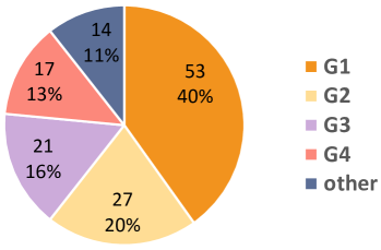
(a) Informative plans

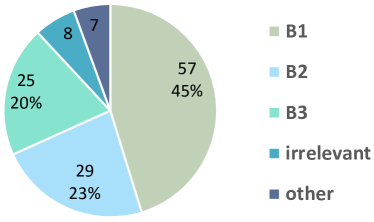
(b) Uninformative plans

Figure 2: Survey results.

Feedback from volunteers. The above example illustrates that the content, structure, and cost of a query plan w.r.t. the qep and already-viewed plans play pivotal roles in determining informativeness of aqps. To further validate this, we survey 68 unpaid volunteers who have taken a database systems course recently or currently taking it in an academic institution. Specifically, they are either current undergraduate students in a computer science degree program or junior database engineers who have recently joined industry. Note that we focus on this group of volunteers as a key application of arena is in database education.

We choose aqps of two sql queries on the IMDb dataset for the volunteers to provide feedback. These queries contain 3-4 joins and involve different table scan methods. Note that randomly selecting a large number of alternative plans for feedback is ineffective as they not only may insufficiently cover diverse types of plans w.r.t. the qeps of the queries but also our engagement with the volunteers reveal that it may deter them to give feedback as they have to browse a large number of plans. Hence, for each query, we display the qep and 8 alternative plans, which are heuristically selected by evaluating their differences w.r.t. the qep based on three dimensions, i.e., structure, content, and estimated cost (Table I). For instance, we may choose an alternative plan with small difference in structure or content from the qep but large differences in the other two dimensions. Observe that it covers majority of the aqps of a given query. Note that the heuristic model may occasionally select some similar alternative plans. We deliberately expose these plans to the volunteers to garner feedback on similar alternative plans.

We ask the volunteers to choose the most and least informative plans given a qep and provide justifications for their choices. The aforementioned plan types were not revealed to the volunteers. We received 132 feedbacks from the volunteers. We map the feedbacks on informative and uninformative plans to the plan types in Table I and count the number of occurrences. Fig. 2(a) reports the feedback on plans considered as informative. Specifically, $G_{1}$ represents $AP_{II}$, $G_{2}$ and $G_{3}$ represent plans with lower cost differences. Particularly, $G_{2}$ are plans with large structure and content differences ($AP_{VII}$) whereas $G_{3}$ are those that have small structural or content differences ($AP_{III}$, $AP_{IV}$). $G_{4}$ represents $AP_{VI}$ and $AP_{VIII}$. There are other feedbacks that are too sparse to be grouped as representative of the volunteers.

Fig. 2(b) reports the feedback on uninformative plans selected by the volunteers. $B_{1}$ represents plans that are very similar to the qep ($AP_{I}$) and hence voted as uninformative as they do not convey any useful information. $B_{2}$ represents $AP_{VI}$ and $AP_{VIII}$. $B_{3}$ are plans that are very similar to other alternative plans viewed by the volunteers. In addition, there are eight other feedbacks that are orthogonal to our problem (i.e., feedback on the visual interface design) and hence categorized as “irrelevant”.

Summary. Our engagement with volunteers reveal that majority find alternative plans of types $AP_{II}-AP_{IV}$ and $AP_{VII}$ informative. However, $AP_{I}$, $AP_{V}$, $AP_{VI}$, and $AP_{VIII}$ are not. Observe that the number of feedbacks for the latter two that deem them uninformative is significantly more than those that consider them informative ($G_{4}$ vs $B_{2}$). Hence, we consider them uninformative. Volunteers also find similar alternative plans uninformative. In the sequel, we shall use these insights to guide the design of plan informativeness and pruning strategies.

III Informative Plan Selection (TIPS) Problem

In this section, we formally define the tips problem. We begin with a brief background on relational query plans.

III-A Relational Query Plans

Given an arbitrary sql query, an rdbms generates a query execution plan (qep) to execute it. A qep consists of a collection of physical operators organized in form of a tree, namely the physical operator tree (operator tree for brevity). Fig. 1(a) depicts an example qep. Each physical operator, e.g., SEQUENTIAL SCAN, INDEX SCAN, takes as input one or more data streams and produces an output one. A qep explicitly describes how the underlying rdbms shall execute the given query. Notably, given a sql, there are many different query plans, other than the qep, for executing it. For instance, there are several physical operators in a rdbms that implement a join, e.g., HASH JOIN, SORT MERGE, NESTED LOOP. We refer to each of these different plans (other than the qep) as an alternative query plan (aqp). Fig. 1(b)-(d) depict three examples of aqp. It is well-known that the plan space is non-polynomial [7].

III-B Problem Definition

The informative plan selection (tips) problem aims to automatically select a small number of alternative plans that maximize plan informativeness. These plans are referred to as informative alternative plans (informative plans/aqps for brevity). The tips problem has two flavors:

• Batch tips. A user may wish to view top-$k$ informative plans beside the qep;

• Incremental tips. A user may iteratively view an informative plan besides what have been already shown to him/her;

Formally, we define these two variants of tips as follows.

Definition III.1

Given a qep $\pi^{*}$ and a budget $k$, the batched informative plan selection (b-tips) problem aims to find top-$k$ alternative plans $\Pi_{OPT}$ such that the plan informativeness of the plans in $\Pi_{OPT}\cup\{\pi^{*}\}$ is maximized, that is

$$\Pi_{OPT}=\operatorname*{argmax}_{\Pi}U(\Pi\cup\{\pi^{*}\})~{}\text{s.t.}~{}|\Pi|=k~{}\text{and}~{}\Pi\subseteq\Pi^{*}\setminus\{\pi^{*}\}$$

where $\Pi^{*}$ denotes the space of all possible plans and $U(\cdot)$ denotes the plan informativeness of a set of query plans.

Definition III.2

Given a query plan set $\Pi$ a user has seen so far, the iterative informative plan selection (i-tips) problem aims to select an alternative plan $\pi_{OPT}$ such that the plan informativeness of the plans in $\Pi\cup\{\pi_{OPT}\}$ is maximized, that is

$$\pi_{OPT}=\operatorname*{argmax}_{\pi}U(\Pi\cup\{\pi\})\mbox{ subject to }\pi\in\Pi^{*}\mbox{ and }\pi\notin\Pi$$

In the next section, we shall elaborate on the notion of plan informativeness $U(\cdot)$ to capture informative plans.

Example III.3

Reconsider Example I.1. Suppose Lena has viewed the qep in Fig. 1(a). She may now wish to view another two alternative plans (i.e., $k=2$) that are informative. The b-tips problem is designed to address it by selecting these alternative plans from the entire plan space so that the plan informativeness $U(\cdot)$ of the qep and the selected plans is maximized. On the other hand, suppose another learner is unsure about how many alternative plans should be viewed or is dissatisified with the result returned by b-tips. In this case, the i-tips problem enables him to iteratively select “aqp-at-a-time” and provide a rating w.r.t. its informativeness until satisfied. The plan informativeness is maximized by considering the rating from the learner.    

Given a plan informativeness measure $U(\cdot)$ and the plan space $\Pi^{\ast}$, we can find an alternative plan for the i-tips problem in $O(|\Pi^{\ast}|)$ time. However, plan space increases exponentially with the increase in the number of joins and it is NP-hard to find the best join order [21]. Therefore, we need efficient solutions especially when there is a large number of joined tables.

Theorem III.4

Given a plan informativeness measure $U(\cdot)$, b-tips problem is NP-hard.

Proof:

(Sketch). Let us consider the facility dispersion problem which is NP-hard [36]. In that problem, one is given a facility set $S$, a function $f$ of distance and an integer $k(k<|F|)$. The objective is to find a subset $S^{\prime}(|S^{\prime}|=k)$ of $S$ so that the given function on $f$ is maximum. Because facility dispersion problem is a special case of b-tips where $\{\pi^{*}\}=\emptyset$ and $U(\cdot)=f$, b-tips is also NP-hard. ∎

IV Quantifying Plan Interestingness

In this section, we describe the quantification of plan informativeness $U(\cdot)$ introduced in the preceding section by exploiting the insights from learner-centered characterization of aqps in Section II.

IV-A Lessons from Characterization of AQPs

In Section II, feedbacks from volunteers reveal that the selection of informative plans is influenced by the followings: (a) The structure, content, and cost differences of an alternative plan w.r.t. the qep (and other alterative plans) can be exploited to differentiate between informative and uninformative alternative plans. Hence, we need to quantify these differences for informative plan selection. (b) Volunteers typically do not prefer to view alternative plans that are very similar to the qep or other alternative plans already viewed by them. We now elaborate on the quantification approach to capture two factors and then utilizing them to quantify plan interestingness.

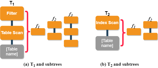
Figure 3: Plan Tree examples.

IV-B Plan Differences

Broadly, $U(\cdot)$ should facilitate identifying specific alternative plans other than the qep such that by putting them together a user can acquire a comprehensive understanding of the alternative plan choices made by a query optimizer for her query (i.e., informative). This entails quantifying effectively differences between different plans w.r.t. their structure, content, and estimated cost. As $U(\cdot)$ is defined over a set of query plans, we shall first discuss the approach of quantifying these differences.

Structural Difference. To evaluate the structural difference between a pair of physical operator trees, we need to employ a measure to compute structural differences between trees. The choice of this measure is orthogonal to our framework and any distance measure that can compute the structural differences between trees efficiently can be adopted. By default, we use the subtree kernel, which has been widely adopted for tree-structured data [39] to measure the structural difference. Formally, a kernel function [38] is a function measuring the similarity of any pair of objects $\{x,x^{\prime}\}$ in the input domain $\mathcal{X}$. It is written as $\kappa(x,x^{\prime})=\left<\phi(x),\phi(x^{\prime})\right>$, in which $\phi$ is a mapping from $\mathcal{X}$ to a feature space $\mathcal{F}$. The basic idea of subtree kernel is to express a kernel on a discrete object by a sum of kernels of their constituent parts. The features of the subtree kernel are proper subtrees of the input tree $T$. A proper subtree $f_{i}$ comprises node $n_{i}$ along with all of its descendants. Two proper subtrees are identical if and only if they have the same tree structure. For example, consider $T_{1}$ and $T_{2}$ in Fig. 3. $T_{1}$ has three different proper subtrees, while $T_{2}$ only has two subtrees. They share two of them, namely, $f_{1}$, $f_{2}$. Note that we do not consider the content of nodes here. Formally, subtree kernel is defined as follows.

Definition IV.1

Given two trees $T_{a}$ and $T_{b}$, the subtree kernel is:

$$\kappa_{S}\left(T_{a},T_{b}\right)=\sum_{n_{a}\in N(T_{a})}\sum_{n_{b}\in N(T_{b})}\Delta(n_{a},n_{b})$$

where $\Delta(n_{a},n_{b})=\sum_{i=1}^{|\mathcal{F}|}I_{i}(n_{a})I_{i}(n_{b})$, and where $I_{i}(n)$ is an indicator function which determines whether the proper subtree $f_{i}$ is rooted at node $n$ and $N(T)$ denotes the node set of $T$.

For example, the kernel score in Fig. 3 is $\kappa_{S}(T_{1},T_{2})=1\times 1+1\times 1=2$ because they share the substructures $f_{1}$, $f_{2}$. Since the subtree kernel is a similarity measure, we need to convert it to a distance. Moreover, each dimension may have different scale. Hence, it is necessary to normalize each distance dimension. For subtree kernel $\kappa\left(T_{a},T_{b}\right)$, we first compute the normalized kernel as follows and then define the structural distance:

$$\kappa\left(T_{a},T_{b}\right)=\kappa_{S}(T_{a},T_{b})/\sqrt{\kappa_{S}(T_{a},T_{a})\cdot\kappa_{S}(T_{b},T_{b})}$$

Definition IV.2

Given two query plans $\pi_{a},\pi_{b}$ with corresponding tree structures $T_{a},T_{b}$, based on the normalized kernel, we can define the structural distance between the plans as

$$s\_dist\left(\pi_{a},\pi_{b}\right)=\sqrt{1-\kappa\left(T_{a},T_{b}\right)}$$

Lemma IV.3

The structural distance is a metric.

Proof:

Subtree kernel $\kappa_{S}\left(T_{a},T_{b}\right)$ is a valid kernel and we map the tree to one metric space. Consequently, we define a norm $||T||=\sqrt{\kappa\left(T,T\right)}$ based on the normalized kernel, and then the $L_{2}$ distance metric on this space is

$$L_{2}(T_{a},T_{b}) =||T_{a}-T_{b}||$$

$$=\sqrt{\kappa(T_{a},T_{a})+\kappa(T_{b},T_{b})-2\kappa(T_{a},T_{b})}$$

$$=\sqrt{2\left(1-\kappa(T_{a},T_{b})\right)}$$

The above deduction relies on $\kappa(T_{a},T_{a})=\kappa(T_{b},T_{b})=1$. Finally, we conclude the $s\_dist(T_{a},T_{b})$ is a metric since $L_{2}(T_{a},T_{b})=\sqrt{2}s\_dist(T_{a},T_{b})$. ∎

It is worth noting that classical approach of computing subtree kernel using suffix tree will lead to quadratic time cost [39]. We advocate that this will introduce large computational cost in our problem scenario since we need to build a suffix tree for each alternative plan at runtime. To address this problem, we first serialize a tree bottom-up, and then use a hash table to record the number of different subtrees. When calculating the subtree kernel, we can directly employ a hash table to find the same subtree. Although the worst-case time complexity is still quadratic, as we shall see in Section VII, it is significantly faster than the classical suffix tree-based approach in practice.

Content Difference. In order to further compare the content of the nodes, we adopt the edit distance to quantify content differences. Specifically, we first use the preorder traversal to convert a physical operator tree to a string, and based on it we apply the edit distance. Note that the alphabet is the collection of all node contents and the content of each tree node is regarded as the basic unit of comparison. For instance, in Fig. 3, the strings of $T_{1}$ and $T_{2}$ are [“Filter”, “Table Scan[Table name]”] and [“Index Scan[Table name]”], respectively. The edit distance is 2 as they require at least two inserts/replaces to become identical to each other.

Since we want to ensure that the content distance is a metric, we further normalize the edit distance [27]. Let $\Sigma$ be the alphabet, $\lambda\notin\Sigma$ is the null string and $\gamma$ is a non-negative real number which represents the weight of a transformation. Given two strings $X,Y$, the normalized edit distance is

$$edit_{norm}(X,Y)=\frac{2\cdot edit(X,Y)}{\alpha\cdot(|X|+|Y|)+edit(X,Y)}$$

where $\alpha=\max\{\gamma(a\rightarrow\lambda),\gamma(\lambda\rightarrow b),a,b\in\sum\}$ and $|X|$ is the length of $X$. This is proven to be a metric [27]. In our work, $\gamma=1$. So the content distance can be defined as follows.

Definition IV.4

Given two query plans $\pi_{a},\pi_{b}$ and the corresponding strings $X_{a},X_{b}$, the content distance between the plans is defined as

$$c\_dist(\pi_{a},\pi_{b})=\frac{2\cdot edit(X_{a},X_{b})}{|X_{a}|+|X_{b}|+edit(X_{a},X_{b})}.$$

Notably, join order difference is a special case where the content is the same while the order is different. Obviously, Defn. IV.4 is able to differentiate different join orders, e.g., AP1 and AP2 in Fig. 1(b) and 1(c). It is easy to infer that the distance presented above is able to differentiate these two plans.

(a) Categories of aqps

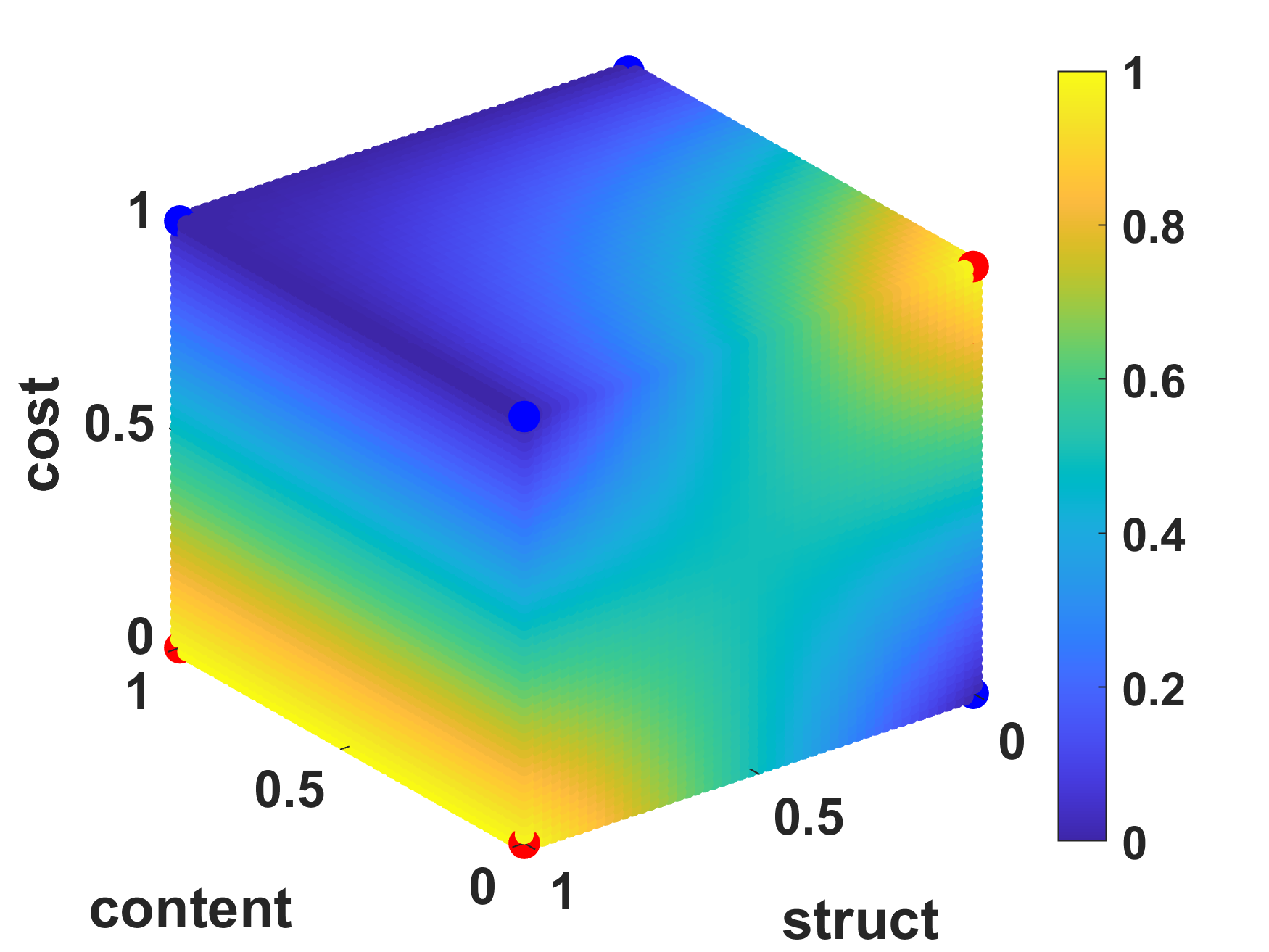
(b) Effect of the fitted function

Figure 4: Relevance.

Remark. There exist several different ways to define the distance between structure and content. But they are not suitable for solving our problems. For example, we could extract a finite-length feature vector for each plan, and then map it to a feature space to calculate the similarity via dot product. We have implemented this approach and conducted comparisons, which will be shown in Section VII.

Cost Difference. Finally, because the (time) cost is a real number, we can adopt $L1$ distance and apply Min-Max normalization accordingly. In all, we are now ready to present the definition of distance:

Definition IV.5

Given two plans $\pi_{a},\pi_{b}$ and the corresponding costs $cost_{a},cost_{b}$, the cost distance between the plans is defined as

$$cost\_dist(\pi_{a},\pi_{b})=\frac{|cost_{a}-cost_{b}|}{cost_{max}-cost_{min}}.$$

Definition IV.6

Given two query plans $\pi_{i},\pi_{j}$, the distance between them is

$$dist(\pi_{i},\pi_{j})=\alpha\cdot s\_dist(\pi_{i},\pi_{j})+\beta\cdot c\_dist(\pi_{i},\pi_{j})+$$

$$(1-\alpha-\beta)\cdot cost\_dist(\pi_{i},\pi_{j})$$

where $0\leq\alpha,\beta\leq 1$ are pre-defined weights.

IV-C Relevance of an Alternative Plan

The aforementioned distance measures enable us to avoid choosing plans with structure, content, and cost differences that are inconsistent with the feedbacks from volunteers. They can prevent selection of an alternative plan that is similar to plans that have been already viewed by a user. However, these measures individually cannot distil informative plans from uninformative ones. Therefore, we propose another measure called relevance (denoted as $rel(\cdot)$), to evaluate the “value” of each plan, such that informative plans receive higher relevance scores. Recall from Section II the 8 types of alternative plans. We convert the differences in these types into binary form (Fig. 4(a)) where 1 indicates large. We can also represent the informative value of these types (based on learner feedback) in binary form (1 means informative). We can then employ a multivariate function fitting to find an appropriate relevance function such that alternative plans that are close to the informative ones receive high scores. Since 8 existing samples are insufficient for fitting a polynomial function with an order higher than 3 [22], it should appear in the following form: $\rho_{1}\times s+\rho_{2}\times c+\rho_{3}\times cost+\rho_{4}\times s\times c+\rho_{5}\times s\times cost+\rho_{6}\times c\times cost+\rho_{7}\times s\times c\times cost$ where $\rho_{1},\ldots,\rho_{7}$ are parameters to be fit. By fitting the above polynomial, we can define the relevance measure as follows.

Definition IV.7

Given the normalized structure distance $s_{i}$, content distance $c_{i}$ and cost distance $cost_{i}$ between an alternative plan $\pi_{i}$ and the qep $\pi^{*}$, the relevance score of $\pi_{i}$ is defined as

$$rel(\pi_{i})=s_{i}+c_{i}+cost_{i}-s_{i}\cdot c_{i}-2\cdot s_{i}\cdot cost_{i}-2\cdot c_{i}\cdot cost_{i}+2\cdot s_{i}\cdot c_{i}\cdot cost_{i}.$$

The effect of $rel(\cdot)$ is shown in Fig. 4(b). The red vertices represent the plan types that learners consider the most informative, which can effectively be captured by $rel(\cdot)$. In addition, plans close to the informative ones receive high scores accordingly. In fact, each plan $\pi$ can be referred to as a 3-dimensional vector $\vec{\pi}$ in the space shown in Fig. 4(b), hence $rel(\cdot)$ transforms a vector to a scale value, we shall use $rel(\pi)$ instead of $rel(\vec{\pi})$ for short.

Remark. Note that the distance and relevance scores are different. The former evaluates the differences between plans, while the latter is used to assign a higher score to aqps that users consider informative. Any lower-order polynomial cannot satisfy this requirement. More importantly, these measures are generic and orthogonal to the distribution of plan categories and the characterization approach of informative alternative plans in specific applications.

IV-D Plan Interestingness

Intuitively, through the plan interestingness measure, we aim to maximize the minimum relevance and distance of the selected query plan set. To this end, we can exploit measures that have been used in diversifying search results such as MaxMin, MaxSum, DisC, etc. [10; 11]. An experimental study in [12] has reported the effect of these choices in diversifying search results. Specifically, MaxSum and k-medoids fail to cover all areas of the result space; MaxSum tends to focus on the outskirts of the results whereas k-medoids clustering reports only central points, ignoring sparser areas. MaxMin and DisC perform better in this aspect. However, in the DisC model, users need to select a radius $r$ instead of the number $k$ of diverse results [11]. As the distribution of plans is uncertain, it is difficult to choose a suitable radius for the DisC model. Hence, we utilize the MaxMin model.

Suppose the plan set is $\Pi$. Then the objective is to maximize the following condition where $\lambda>0$ is a parameter specifying the trade-off between relevance and distance.

$$(1-\lambda)\min\limits_{\pi_{i}\in\Pi}rel(\pi_{i})+\lambda\min\limits_{\pi_{i},\pi_{j}\in\Pi}dist(\pi_{i},\pi_{j})$$ (1)

Definition IV.8

Given two query plans $\pi_{i},\pi_{j}$, the refined distance function is

$$Dist(\pi_{i},\pi_{j})=\frac{(1-\lambda)}{2}(rel(\pi_{i})+rel(\pi_{j}))+\lambda dist(\pi_{i},\pi_{j}).$$

Lemma IV.9

The distance function defined in Definition IV.8 satisfies the triangle inequality.

Proof:

$dist(\cdot)$ is a linear combination of $s\_dist$, $c\_dist$ and $cost\_dist$. Because all of them is metric, $dist(\cdot)$ is a metric too. $dist(\cdot)$ satisfies the triangle inequality. Then we only need to prove that $\frac{1-\lambda}{2}\left(rel(a)+rel(b)\right)$ satisfies the triangle inequality. Let $R(a,b)=rel(a)+rel(b)$, then

$$R(a,b)+R(a,c) =rel(a)+rel(b)+rel(a)+rel(c)$$

$$=2\cdot rel(a)+rel(b)+rel(c)$$

$$=2\cdot rel(a)+R(b,c)$$

Since $rel(a)\geq 0$, $R(a,b)+R(a,c)\geq R(b,c)$. Similarly, we can prove that $R(a,b)-R(a,c)\leq R(b,c)$. Therefore the $Dist(\cdot)$ consists of $R(\cdot)$ and $dist(\cdot)$ also satisfies the triangle inequality. ∎

According to [15], the above bi-criteria objective problem can be transformed to find the refined distance defined in Definition IV.8. Consequently, we can define the plan interestingness $U(\cdot)$ as follows.

Definition IV.10

Given a query plan set $\Pi$, the plan interestingness is defined as $U(\Pi)=\min{Dist(\pi_{i},\pi_{j})}$ where $\pi_{i}\in\Pi,\pi_{j}\in\Pi.$

Now we consider $U_{r}$ in Defn. III.2, notably, i-tips allows a user to explore AP iteratively based on what has been revealed so far. We take into account the user preference in the form of $r\in\{1,0\}$ (i.e., prefer or not) during the exploration. For example, a user may want to find only those plans with different join orders but not others. This scenario can be easily addressed by i-tips, which allows one to mark whether a newly generated plan is preferred. Consider Fig. 4b where each AP is represented as a 3-dimensional vector $\vec{\pi}$ w.r.t. the qep ($\vec{\pi^{*}}=\langle 0,0,0\rangle$). According to Defn. IV.7, a preferred AP (as well as its neighbors) should receive higher relevance scores (warmer in the heatmap). Intuitively, finding the category of the preferred AP (i.e., $AP_{II}\sim AP_{IV},AP_{VII}$), say $AP_{II}$ (according to Fig. 4a, we can denote $\vec{AP_{II}}=\langle 0,0,1\rangle$), and moving the next plan towards (resp., away from) it if $r=1$ (resp., $r=0$), e.g., $\vec{\pi}=\vec{\pi}+\epsilon(\vec{AP_{II}}-\vec{\pi})$ would address this ($\epsilon=0.05$ by default). However, this strategy can affect only a single AP in the current iteration but not later. Therefore, instead of moving a single AP, we select to update the origin of the 3-dimensional system, i.e., $\vec{\pi^{*}}=\vec{\pi^{*}}-\epsilon(\vec{AP_{pre}}-\vec{\pi})$, where $\pi$ refers to the latest plan seen so far, and $AP_{pre}$ refers to the category to which $\pi$ belongs. To find $AP_{pre}$ for a plan $\pi$, we only need to perform a nearest neighbor search over the set of $\{\vec{AP_{II}},\vec{AP_{III}},\vec{AP_{IV}},\vec{AP_{VII}}\}$ (each can be encoded according to Fig. 4a) with respect to $\vec{\pi}$.

V The ARENA Framework

In this section, we present arena, an end-to-end framework for exploring informative alternative plans. The architecture of arena is shown in Fig. 5. It consists of the following components.

arena GUI. A browser-based visual interface that enables a user to retrieve and view information related to the qep and alternative query plans of her input query in a user-friendly manner. Once an sql query is submitted by a user, the corresponding qep is retrieved from the rdbms, based on which she may either invoke the b-tips or the i-tips component (detailed in Section VI).

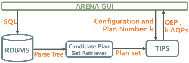
Figure 5: Architecture of arena.

Candidate Plan Set Retriever. In order to obtain the plan space for a given sql query (i.e., $\Pi^{*}$), we investigate a series of existing tools including [17; 16; 28; 30; 42; 40] and finally we decided to adopt orca [40]. orca is a modular top-down query optimizer based on the cascades optimization framework [16]. We adopt it in arena for the following reasons. First, it is a stand-alone optimizer and is independent of the rdbms a learner interacts with. Consequently, it facilitates portability of arena across different rdbms. Second, it interacts with the rdbms through a standard xml interface such that the effort to support a new rdbms is minimized. The only task one needs to undertake is to rewrite the parser that transforms a new format of query plan (e.g., xml in SQL Server, json in PostgreSQL) into the standard xml interface of orca. Consequently, this makes arena compatible with majority of rdbms as almost all of them output a qep in a particular format such that a parser can be easily written without touching the internal of the target rdbms. It is worth noting that the choice of implementation is orthogonal here. Other frameworks with similar functionality can also be adopted.

In order to implement the orca interface, we write all the information required by orca into an xml file, and then call the function in orca to read it for optimization. The xml file mainly consists of two parts: (a) the sql query and (b) statistical information related to the query. For further information, please refer to  [40] and its source code (https://github.com/greenplum-db/gporca). As a proof of concept, we have implemented this interface on top of PostgreSQL and Greenplum.

tips. The candidate plans from the above module are passed to the tips module. It implements the solutions proposed in the next section to retrieve the set of $k$ alternative query plans.

VI TIPS Algorithms

Recall from Section 1, we cannot integrate the selection of informative plans into the enumeration step of the query optimizer as these plans are selected based on the qep and aqps a learner have seen. Additionally, query optimizers search and filter on the basis of cost. In contrast, arena is neither seeking a single plan nor plans with the smallest cost. Hence, tips requires novel algorithms. Specifically, we present i-tips and b-tips to address the two variants of the problem introduced in Section III. We begin by introducing two pruning strategies that are exploited by them. Note that all these algorithms take as input a collection of candidate aqps $\Pi^{\ast}$ that is retrieved by arena from the underlying rdbms as detailed in Section V.

VI-A Group Forest-based Pruning (GFP)

Give that the plan space can be very large for some queries, traversing all aqps to select informative plans can adversely impact efficiency of our solutions. Therefore, we need a strategy to quickly filter out uninformative aqps. According to feedbacks from volunteers (Section II), $AP_{VI}$ and $AP_{VIII}$ in Table I are uninformative. Observe that both these categories of plans have significant structural differences w.r.t. the qep. Hence, a simple approach to filter uninformative plans is to calculate the difference between each aqp and the qep and then discard aqps with very large differences. Although this approach can reduce the number of plans, we still need to traverse the entire plan space for computing the differences. Hence, we propose a group forest-based pruning strategy, which can not only reduce the number of aqps but also avoid accessing the entire plan space during the pruning process.

1

Input: qep $\pi^{\ast}$, collection of all aqps $\Pi^{\ast}$

Output: sampling of $\Pi^{\ast}$

2 $\Pi_{1}\leftarrow\emptyset$;

3 for $\pi_{i}$ in $\Pi^{\ast}$ do

4       if $s\_dist(\pi_{i},\pi^{*})=0$ then

5            $\Pi_{1}=\Pi_{1}\cup\{\pi_{i}\}$

6       end if

7      

8 end for

9

10$\Pi_{2}=UniformSampling(\Pi^{\ast})$;

11 return $\Pi_{1}\cup\Pi_{2}$;

Algorithm 1 Algorithm ips

Cascade optimizers [16] utilize a memo structure (i.e., a forest of operator trees) to track all possible plans. A memo consists of a series of groups, each of which contains a number of expressions. An expression is employed to represent a logical/physical operator. Fig. 6a depicts an example of a memo, where each row represents a group and the square represents an expression in it. Each expression is associated with an id in the form of ‘GroupID.ExpressionID’, shown at the lower left corner (e.g., 3.1, 2.1). The lower right corner of an expression shows the id(s) of the child group(s) it points to. Different expressions in the same group are different operators that can achieve the same functionality. For example, both 3.1 (HashJoin) and 3.2 (NTLoop) implement the join operation. Suppose Group 3 is the root group. When we traverse down from the expression in the root group, we can get a plan. For example the id sequence (3.1, 2.1, 1.1) represents the plan HashJoin[TableScan, TableScan]. The upper right corner of each expression records the number of alternatives with this expression as the root node. For example, the number of expression 1.3 is 2, which includes 1.3$\rightarrow$1.1 and 1.3$\rightarrow$1.2.

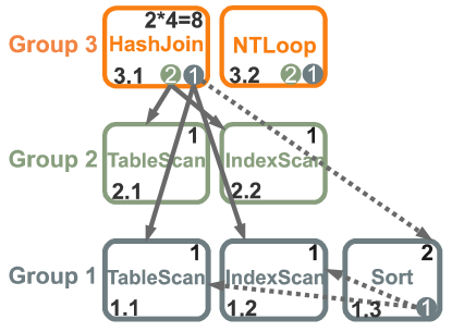
(a) MEMO Structure.

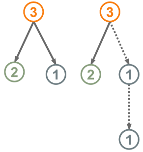
(b) Group Forest.

Figure 6: Example of MEMO and Group Forest.

Observe that the number of alternatives of the expression 3.1 in the root node is 8. That is, there are 8 different plans rooting at expression 3.1. However, there are only 2 tree structures over all these 8 plans as shown in Fig.  6b. The number in each node represents the id of the group. Since these trees represent connections between different groups, we refer to them collectively as group forest. Each group tree in a group forest represents multiple plans with the same structure and if the structure distance of a group tree and the qep is larger than a given distance threshold $\tau_{d}$, i.e., $s\_dist(\pi,\pi^{*})\geq\tau_{d}$, all the corresponding ids can be filtered out. Observe that the number of group trees is significantly smaller than the number of aqps. Therefore, uninformative plans can be quickly eliminated by leveraging them. In order to construct the group forest, we only need to traverse the memo in a bottom-up manner, which is extremely fast, i.e., time cost is linear to the height of the constructed tree.

Lastly, observe that if we filter based on $s\_dist$ only, informative plans of types $AP_{IV}$ and $AP_{VII}$ (Table I) may be abandoned. The difference between these two types of plans and $AP_{VI}$ and $AP_{VIII}$ is that the cost is smaller. Hence, we filter using both the structure and cost differences, i.e.,, $s\_dist(\pi,\pi^{*})\geq\tau_{d},cost\_dist(\pi,\pi^{*})\geq\tau_{c}$ where $\tau_{c}$ is a pre-defined cost threshold.

VI-B Importance-based Plan Sampling (IPS)

It is prohibitively expensive to enumerate the entire plan space to select informative plans when the number of joins is large (i.e., involving more than 10 relations). We may sample some plans from the entire plan space and select informative plans from them. However, simply deploying random sampling may discard many informative plans. To address that, we propose an importance-based plan sampling (ips) strategy that exploits the insights gained from feedbacks from volunteers in Section II to select plans for subsequent processing. The overall goal is to preserve the informative plans as much as possible during the sampling. However, retaining all informative plans will inevitably demand traversal of every aqp to compute plan interestingness. Hence, instead of preserving all informative plans, we select to keep the most important ones when the number of joined relations in a query is large. We exploit the feedbacks in Section II to sample plans. Observe that $AP_{II}$ plans receive a significant number of votes among all informative plans. Hence, we inject such plans as much as possible in our sample. Also, $AP_{II}$ plans have small structural differences with the qep. Hence, given a qep, we can easily determine whether an aqp belongs to $AP_{II}$ or not by finding all alternative plans with the same structure as qep. These plans are then combined with uniformly random sampled results. The pseudocode of the ips strategy is shown in Algorithm 1.

1

Input: qep $\pi^{*}$, collection of all aqps $\Pi^{*}$, ips threshold $\tau_{\ell}$, gfp threshold $\tau_{g}$

Output: an alternative informative query plan $\pi^{(i)}$ during iteration $i$

2

3if the number of join tables ¿ $\tau_{\ell}$ then

4      $\Pi^{*}=$ ips($\pi^{*}$, $\Pi^{*}$);

5      

6 end if

7

8if  $|\Pi^{*}|>\tau_{g}$ then

      $\Pi^{*}=$gfp($\pi^{*}$, $\Pi^{*}$) // Group forest-based pruning

9      

10 end if

11At iteration $i$;

12 if $\pi^{(i-1)}$ in last iteration is marked preferred then

13       $AP_{pre}=Cat(\pi^{(i-1)})$;

14       update the origin: $\vec{\pi^{*}}=\vec{\pi^{*}}-\epsilon(\vec{AP_{pre}}-\vec{\pi^{(i-1)}})$;

15 end if

16for $\pi_{j}\in\Pi^{\ast}-\Pi$ do

17       $d_{j}\leftarrow Dist(\vec{\pi_{j}},\vec{\pi^{*}})$

18 end for

19

20Find the plan $\pi^{(i)}\in\Pi^{\ast}-\Pi$ with the maximum $d$;

21 $\Pi=\Pi\bigcup\{\pi^{(i)}\}$;

return $\pi^{(i)}$

Algorithm 2 Algorithm i-tips

VI-C i-tips Algorithm

Algorithm 2 outlines the procedure to address the i-tips problem defined in Definition III.2. If the number of joined relations is greater than the predefined ips threshold $\tau_{\ell}$, we invoke ips (Line 2). In addition, if the number of aqps is greater than the predefined gfp threshold $\tau_{g}$, it invokes the group forest-based pruning strategy (Line 5), to filter out some uninformative plans early.

Notably, i-tips allows a user to explore AP iteratively based on what have been shown. We take into account user-preference during the exploration. For instance, a user may want to find only those plans with different join orders but not others. Such scenario can be easily addressed by i-tips, which enables one to mark whether a newly generated plan is preferred. Consider Fig. 4b where each AP is represented as a 3-dimensional vector $\vec{\pi}$ w.r.t. the qep ($\vec{\pi^{*}}=\langle 0,0,0\rangle$). According to Definition IV.7, a preferred AP (as well as its neighbors) should receive higher relevance scores (warmer in the heatmap). Intuitively, finding the category (Line 9) of the preferred AP (i.e., $AP_{II}\sim AP_{IV},AP_{VII}$), say $AP_{II}$ ($\vec{AP_{II}}=\langle 0,0,1\rangle$), and moving it towards it, e.g., $\vec{\pi}=\vec{\pi}+\epsilon(\vec{AP_{II}}-\vec{\pi})$ would address this ($\epsilon=0.05$ by default). However, this strategy can only affect a single AP in the current iteration but not the ones afterwards. Therefore, instead of moving a single AP, we select to update the origin for the 3-dimensional system, i.e., $\vec{\pi^{*}}=\vec{\pi^{*}}-\epsilon(\vec{AP_{pre}}-\vec{\pi})$ (Line 10), where $AP_{pre}$ refers to the category that $\pi$ belongs to.

1

Input: qep $\pi^{*}$, collection of all aqps $\Pi^{*}$, budget $k$, ips threshold $\tau_{\ell}$, gfp threshold $\tau_{g}$

Output: top-k informative query plans $\Pi$

2

3Lines 1-6 in Algorithm 2;

4

set $Heap$ as a max-heap // record the minimum distance

5 $\Pi\leftarrow\{\pi^{*}\}$

6

7foreach $\pi_{j}\in\Pi^{*}-\{\pi^{*}\}$ do

8       $d\leftarrow Dist(\pi^{*},\pi_{j})$;

9       $Heap.push(tuple(d,\pi_{j}))$;

10      

11 end foreach

12

13while $\left|\Pi\right|\neq k+1$ do

14       set $tmpRecord$ is $\emptyset$;

15       set $optTuple$ is None;

16      

17      while $Heap$ not empty do

18             $tmpTuple\leftarrow Heap.pop()$;

             if $tmpTuple<optTuple$ then // compare distance

19            

20                   break;

21             end if

22            if $tmpTuple$ is not latest then

23                   $tmpTuple\leftarrow Update(tmpTuple)$;

24                  

25             end if

26            if $tmpTuple>optTuple$ then

27                   $optTuple\leftarrow tmpTuple$;

28                  

29             end if

30            $tempRecord.push(tempTuple)$;

31            

32       end while

33      $\Pi\leftarrow\Pi\cup\{optTuple.\pi\}$;

       /* plans that are removed from the heap but not in use are put back into the heap */

34       foreach $t$ in $tmpRecord-\{optTuple\}$ do

35             $Heap.push(t)$ ;

36            

37       end foreach

38      

39 end while

40

return $\Pi-\{\pi^{*}\}$

Algorithm 3 Algorithm b-tips-heap

VI-D b-tips Algorithm

We propose two flavors of the algorithm to address b-tips, namely, b-tips-basic and b-tips-heap.

b-tips-basic algorithm. We can exploit Algorithm 2 to address the b-tips problem. We first add the qep $\pi^{*}$ to the final set $\Pi$. Then iteratively invoke the Algorithm 2 until there are $k+1$ plans in $\Pi$. Each time we just need to add the result of Algorithm 2 to $\Pi$. This algorithm has a time complexity of $O\left(k|\Pi^{\ast}|\right)$.

b-tips-heap algorithm. Since the minimum distance between plans in $\Pi^{*}-\Pi$ and $\Pi$ decrease monotonically with the increase of $|\Pi|$, we can use a max-heap to filter plans with very small distances to avoid unnecessary computation. Algorithm 3 describes the procedure. We first invoke our two pruning strategies (Line 1). In Line 6, we add a tuple which consists of the ID of an alternative plan $\pi$ and a distance to the heap, which indicates the minimum distance between $\pi$ and the plans in $\Pi$. Each time we choose a plan to add into $\Pi$, we do not update the distance of all tuples. Instead, we only need to check if this distance is correct (Line 17) and update it (Line 18). We select the alternative plan with the maximum minimum distance during each iteration. Observe that the worst-case time complexity is also $O\left(k|\Pi^{\ast}|\right)$. However, it is significantly more efficient than b-tips-basic in practice (detailed in Section VII).

For a MaxMin problem, a polynomial-time approximation algorithm provides a performance guarantee of $\rho\geq 1$, if for each instance of the problem, the minimum distance of the result set produced by the algorithm is at least $1/\rho$ of the optimal set minimum distance. We will also refer to such an algorithm as a $\rho$-approximation algorithm.

Theorem VI.1

b-tips algorithms are a 2-approximation algorithm if the distance satisfies the triangle inequality (Lemma IV.9).

Proof:

Suppose $\Pi_{OPT}$ is the optimal solution of the b-tips problem. $OPT=U(\Pi_{OPT}\cup\{\pi^{*}\})$ is the minimum distance. Let $\Pi$ and $\Pi^{\ast}$ represent the result selected by Algorithm 3 and all plans, respectively. Let $f(P)=\min\limits_{x,y\in P}\{Dist(x,y)\}$. We will prove the condition $f(\Pi\cup\{\pi^{*}\})\geq OPT/2$ holds after each addition to $\Pi$. Since $f(\Pi)$ represent the minimum distance of result of Algorithm 3 after the last addition to $\Pi$, the theorem would then follow.

The first addition inserts a plan that is farthest from $\pi^{*}$. There are two cases about $OPT$: $OPT=dist(\pi^{*},\pi_{i})$ or $OPT=dist(\pi_{j},\pi_{i})$ where $\pi_{i},\pi_{j}\neq\pi^{*}$. In either case, $f(\Pi\cup\{\pi^{*}\})>OPT$, Hence, the condition clearly holds after the first addition.

Assume that the condition holds after $k$ additions to $\Pi$, where $k\geq 1$. We will prove by contradiction that the condition holds after the $(k+1)^{th}$ addition to $\Pi$ as well. Let $\Pi_{k}={\pi_{1},\pi_{2},\ldots,\pi_{k},\pi^{*}}$ denote the set $\Pi$ after $k$ additions. Since we are assuming that the above condition does not hold after the $(k+1)^{th}$ addition, it must be that for each $\pi_{j}\in\Pi^{\ast}-\Pi_{k}$, there is a plan $\pi_{i}\in\Pi_{k}$ such that $dist(\pi_{i},\pi_{j})<OPT/2$. We describe this situation by saying that $\pi_{j}$ is blocked by $\pi_{i}$.

Let $\Pi^{\prime}=\Pi_{OPT}\cap(\Pi^{\ast}\setminus\Pi_{k})$. Note that $k<\left|\Pi_{OPT}\right|$ since an additional plan is to be added. Thus $\Pi^{\prime}\geq 1$. It is easy to verify that if $|\Pi^{\prime}|=1$, then the condition will hold after the $(k+1)^{th}$ addition. Therefore, assume that $|\Pi^{\prime}|=r\geq 2$. Furthermore, let $\Pi^{\prime}={y_{1},y_{2},\ldots,y_{r}}$. Since $\Pi^{\prime}\subseteq\Pi_{opt}$, we must have $Dist(y_{i},y_{j})\geq OPT$ for $1\leq i,j\leq r,(i\neq j)$. Since the distances satisfy the triangle inequality (Lemma IV.9), it is possible to show that no two distinct plans in $\Pi^{\prime}$ can be blocked by the same node $\pi_{i}\in\Pi_{k}$. Moreover, if there is a blocking plan in $\Pi_{k}$ that is also in $\Pi_{OPT}$, the minimum distance of $\Pi_{OPT}$ must be smaller than $OPT$, because this is a blocking plan whose minimum distance with $\Pi_{OPT}\setminus\Pi_{k}$ is smaller than $OPT/2$. Therefore, none of the blocking plans in $\Pi_{k}$ can be in $\Pi_{OPT}$ and $|\Pi^{\prime}|=|\Pi_{OPT}|$. It is possible to show that $\Pi_{k}$ must contain $\left|\Pi_{OPT}\right|$ plans to block all plans in $\Pi^{\prime}$. However, this contradicts our initial assumption that $k<\left|\Pi_{OPT}\right|$. Thus, the condition must hold after the $(k+1)^{th}$ addition. ∎

Remark. Our proposed algorithms are generic and not limited to database education. First, they are orthogonal to any candidate plan set retrieval strategy. Second, the strategies gfp and ips are designed based on informative and uninformative plan categories. Although in this paper we focus on categories relevant to database education application, it is easy to see that they can be easily adapted to other applications (e.g., database administration) where potentially different informative and uninformative plan categories may germinate from a human-centered characterization of aqps. It is also easy to be adapted to a non-human-centered characterization of aqps by changing the if-statement in Line 3 of Algorithm 1.

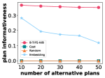
(a) tpch_18

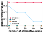
(b) tpch_17

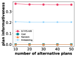
(c) tpch_11

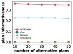
(d) tpch_15

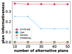
(e) tpch_22

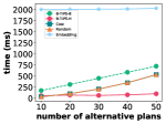
(f) tpch_18

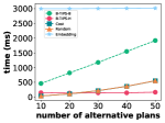
(g) tpch_17

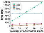
(h) tpch_11

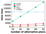
(i) tpch_15

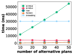
(j) tpch_22

Figure 7: (a-e) Plan informativeness; (f-j) Running time (for the 5 tpc-h queries in the first column of Table II).

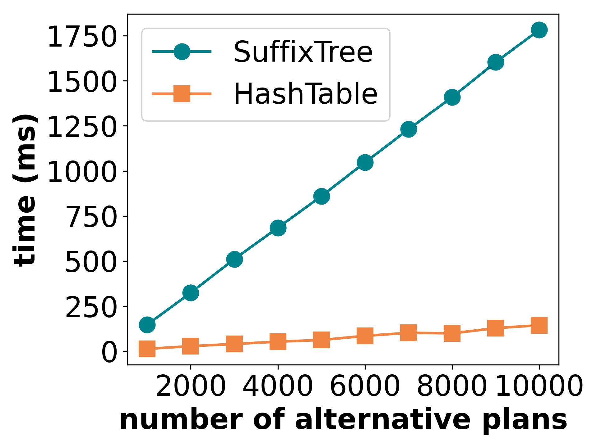
(a) Initialization

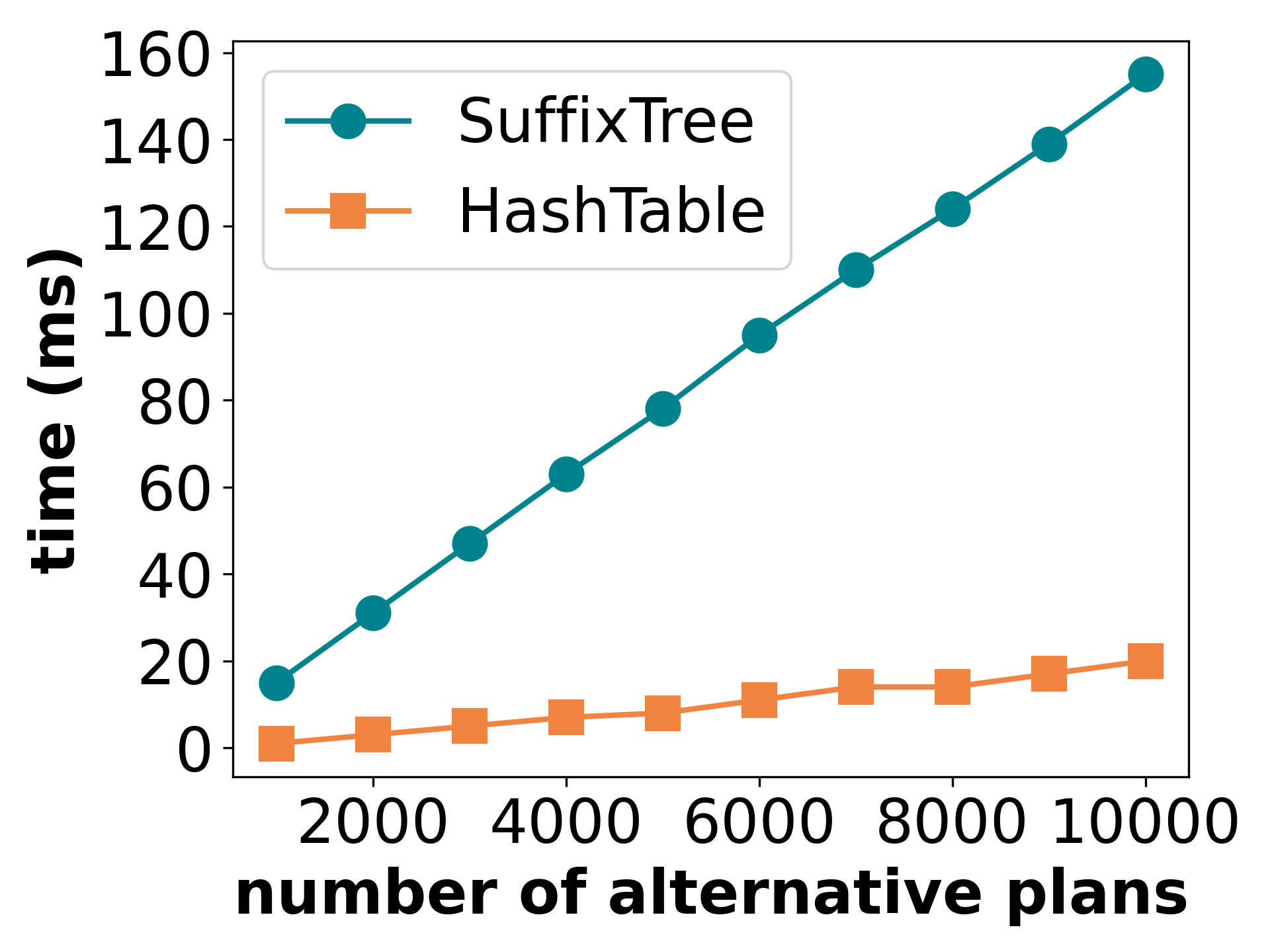
(b) Calculate subtree kernel

Figure 8: Subtree kernel.

VII Performance Study

In this section, we investigate the performance of arena. In the next section, we shall report the usefulness and application of arena in database education.

VII-A Experimental Setup

Datasets. We use two datasets. The first is the Internet Movie Data Base (IMDb) dataset [2; 25], containing two largest tables, cast_info and movie_info have 36M and 15M rows, respectively. The second one is the TPC-H dataset [3]. We use the TPC-H v3 and 1 GB data generated using dbgen [3].

Since the number of candidate plans impacts the performance of tips, which is mainly affected by the sql statement, we choose different sql queries to vary the plan size. For IMDb,  [25] provides 113 sql queries. We choose 8 of them for our experiments. For the TPC-H dataset, there are 22 standard sql statements. Because the uneven distribution of the plan space of these queries, it is difficult to find sql statements that are evenly distributed as in IMDb dataset. We select 6 sql queries from them for our experiments. These selected queries and the plan space size are reported in Table II. Note that the space sizes are the entire plan spaces from orca.

TABLE II: Dataset.

SQL	Space Size	SQL	Space Size
imdb_6b.sql	2059	imdb_6e.sql	10200
imdb_2a.sql	3211	tpch_18.sql	2070
imdb_5c.sql	3957	tpch_17.sql	2864
imdb_2b.sql	4975	tpch_11.sql	11880
imdb_1d.sql	7065	tpch_15.sql	13800
imdb_4b.sql	7887	tpch_21.sql	24300
imdb_1a.sql	9007	tpch_22.sql	51870

Baselines. We are unaware of any existing informative plan selection technique. Hence, we are confined to compare arena with the following baselines. (a) We implemented a random selection algorithm (denoted by random). It is executed repeatedly $n$ times and each time a result is randomly generated. The best result is returned after $n$ iterations. In our experiment, we set $n=30$. (b) A simple solution for tips is to return those with the least cost besides the qep. Hence, we implement a cost-based approach that returns the top-$k$ plans with the least cost in $\Pi^{\ast}$ (denoted by cost) besides the QEP. (c) We also implemented an embedding-based approach (denoted by embedding), where we embed each aqp into a vector by feeding its estimated time cost and tree structure into an autoencoder following [5] and then rank the aqps according to their Euclidean distance w.r.t. the qep. Afterwards, the plan informativeness of the top-$k$ can be computed following Defn. IV.10 accordingly.

All algorithms are implemented in C++ on a 3.2GHz 4-core machine with 16GB RAM. We denote b-tips-basic and b-tips-heap as b-tips-b and b-tips-h, respectively. Unless specified otherwise, we set $\alpha=0.33$, $\beta=0.33$, $\lambda=0.5$, $\tau_{\ell}=10$, and $\tau_{g}=50000$.

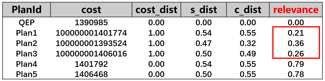
(a) the weight of relevance is 0

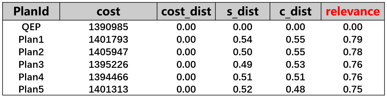
(b) the weight of relevance is 0.5

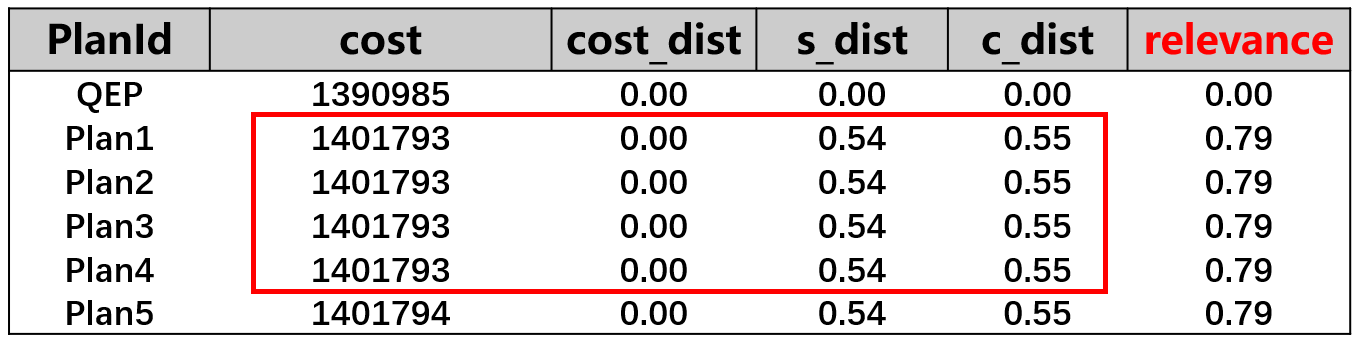
(c) the weight of relevance is 1

Figure 9: Effect of relevance.

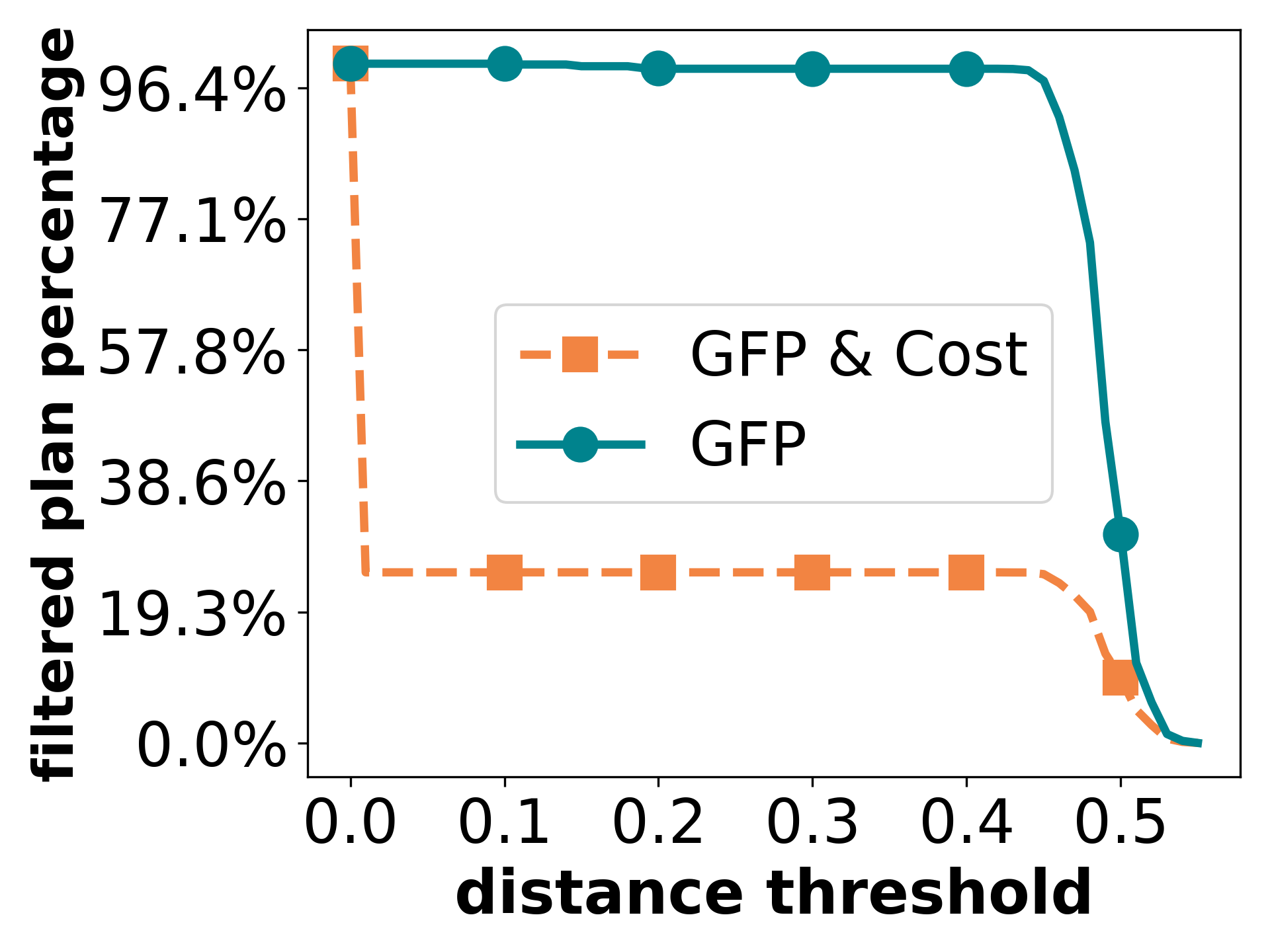
(a) Effect of pruning

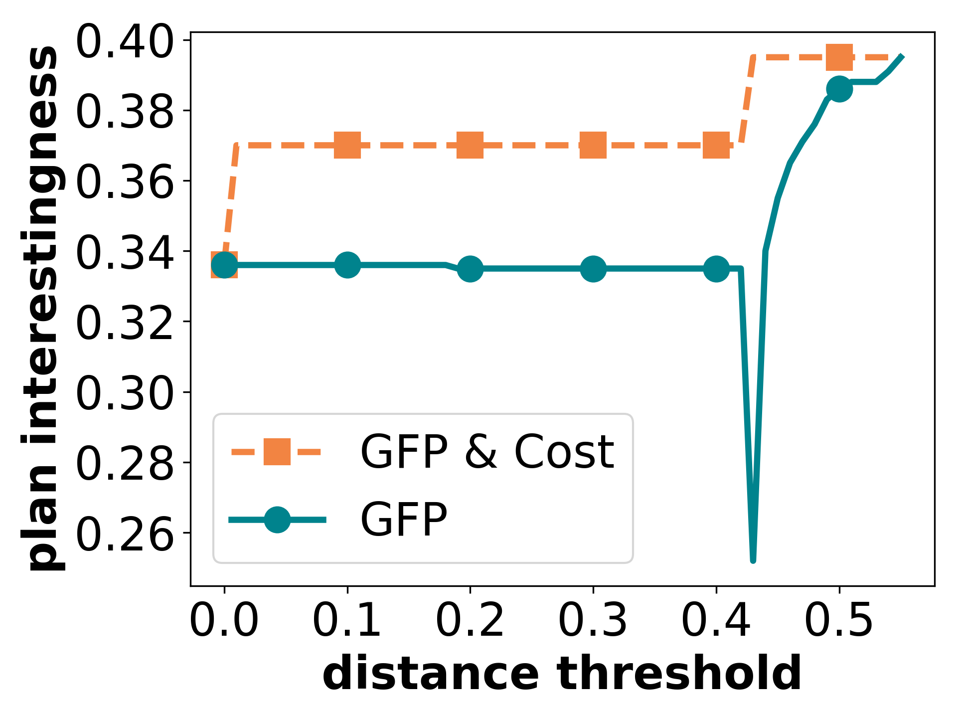
(b) Plan interestingness

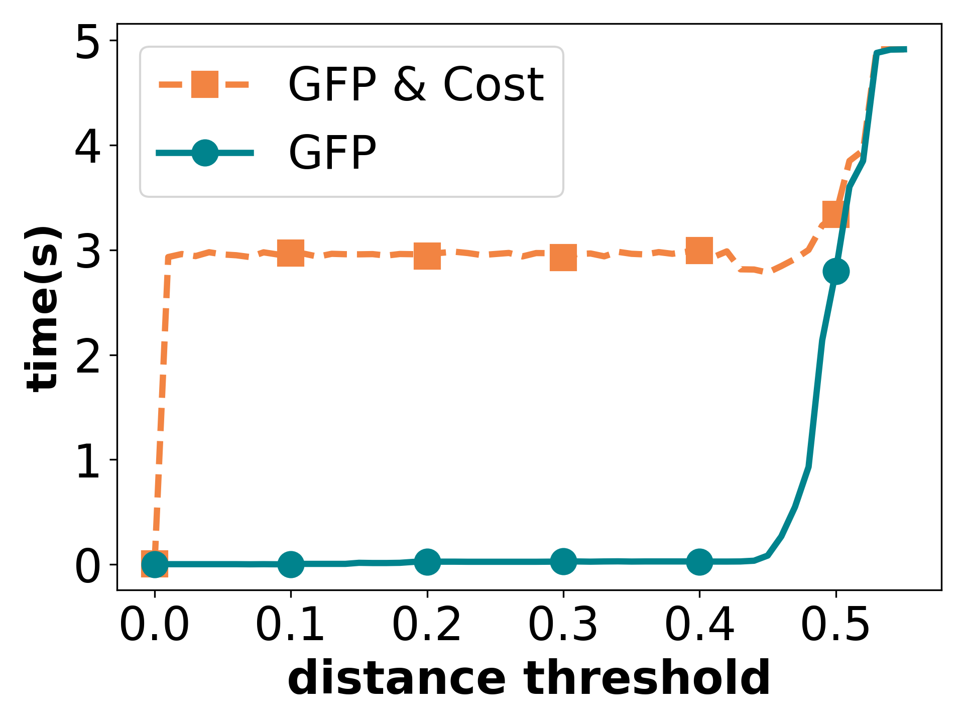
(c) Efficiency

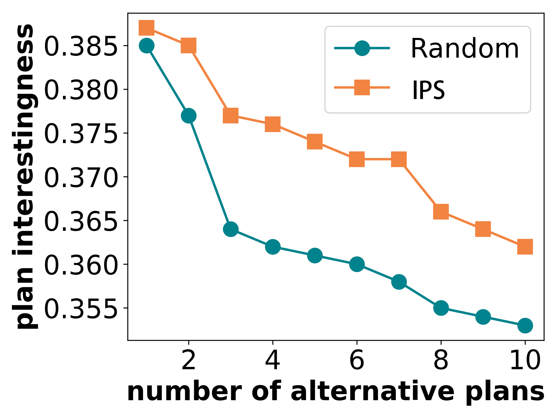
(d) Sample 1000 plans

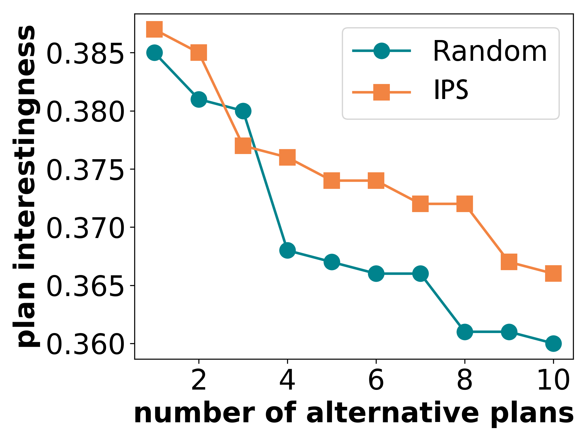
(e) Sample 5000 plans

Figure 10: Pruning strategies: (a,b,c) effect of gfp; (d,e) effect of ips.

VII-B Experimental Results

Exp 1: Efficiency and effectiveness. We first report the efficiency and effectiveness of different algorithms. For each query in Table II, we use different algorithms to select $k$ plans and report the plan informativeness $U$ and runtime, shown in Fig. 7(a-e) and  7(f-j), respectively. We make the following observations. First, the plan informativeness obtained by random, cost and embedding are significantly inferior to that of the b-tips algorithms. Moreover, the effectiveness of embedding decreases with respect to $k$ unless the volume of the plan space is large enough, i.e., $|\Pi^{*}|>10000$. Second, the running time of b-tips-h is closer to cost and random, significantly faster than b-tips-b and embedding, and stable with increasing $k$ due to the heap-based pruning strategy.

Exp 2: Comparison of strategies for subtree kernel. As discussed in Section IV-B, there are two methods to compute the subtree kernel. We compare the efficiency of these two methods in initializing and computing the subtree kernel. The results are reported in Fig. 8. Observe that our hash table-based strategy is consistently more efficient.

Exp 3: Impact of relevance. In this set of experiments, we report the importance of the relevance measure (Defn. IV.7). We set $\lambda$ to 0, 0.5, and 1, and use b-tips to select 5 aqps. The results are shown in Fig. 9. When $\lambda=0$ (resp., $\lambda=1$), $U$ is only composed of relevance (resp., distance). Hence, in Fig. 9LABEL:sub@subfig:relevance_0, the selected plans differ much from qep but have a small relevance. In Fig. 9LABEL:sub@subfig:relevance_1, the selected plans have a high relevance value but exhibit a smaller difference. Based on the learner-centric characterization of aqps in Section II, both of these cases are not desirable. When $\lambda=0.5$, $U$ is composed of distance and relevance. Furthermore, it can be seen from Fig. 9LABEL:sub@subfig:relevance_5 that when relevance and distance are considered together, these values are relatively reasonable and there is no case where a certain value is particularly small. The selected plans are not similar, while displaying large relevance. Therefore, this result is more reasonable and informative.

Exp 4: Impact of gfp strategy. Now we report the performance of the gfp-based pruning strategy. Fig. 10(a)-(c) plot the results on tpch22.sql, which have a large plan space. We compare the pruning power, plan informativeness, and efficiency of two variants of gfp, one pruned based only on $s\_dist(\cdot)$ and the other with both $s\_dist(\cdot)$ and $cost\_dist(\cdot)$ (referred to as gfp and Cost, respectively). We vary the distance threshold $\tau_{d}$ and set the cost threshold $\tau_{c}=\tau_{d}$. Since the distribution of the plans is not uniform, the curves do not change uniformly. Obviously, pruning based only on $s\_dist(\cdot)$ filters out more plans, but the plan informativeness is worse. If we do not use gfp strategy, the plan informativeness and time cost are 0.395 and 5s, respectively. That is, with gfp and Cost (resp., gfp), by saving more than 40% (resp., 95%) time cost, we may only sacrifice less than 6% (resp., 14%) of the plan informativeness. This justifies the reason for using both $s\_dist(\cdot)$ and $cost\_dist(\cdot)$ in gfp and Cost.

Exp 5: Impact of the ips strategy. We investigate the effect of the ips strategy described in Section VI. We choose 13c.sql in [25] which has 11 joins. We construct two sets of data: (a) We randomly select $n(n=1000,2000,\ldots,5000)$ plans from all the plans currently available as the baseline data. (b) We deploy the ips strategy. We find all alternative plans that have the same structure as qep, add them to the $n$ randomly selected alternative plans. Notably, for a fair comparison, we randomly delete the same number of plans from (b) to ensure that the two sets of data, i.e., (a) and (b), have the same size of plan space. After that, we execute b-tips on the two sets of data and compare the plan informativeness. Fig. 10(c) and  10(d) report the results. Observe that for most cases ips samples plans with higher plan informativeness.

VIII ARENA in Database Education

It is well-established in education that effective use of technology has a positive impact on learning [18]. Technology is best used as “a supplement to normal teaching rather than as a replacement for it” [18]. Hence, learner-friendly tools are often desirable to augment the traditional modes of learning (i.e., textbook, lecture). Indeed, database systems courses in major institutions around the world supplement traditional style of learning with the usage of off-the-shelf rdbms (e.g., PostgreSQL) to infuse knowledge about database techniques used in practice. Unfortunately, these rdbms are not designed for pedagogical support. Although they enable hands-on learning opportunities to build database applications and pose a wide variety of sql queries over it, very limited learner-friendly support is provided beyond it [6]. Specifically, they do not expose a representative set of aqps considered by the underlying query optimizer during the selection of a qep in a user-friendly manner to aid learning. Hence, arena can potentially address this gap by facilitating retrieval and exploration of informative aqps associated with a given query. In this section, we undertake a user study and academic assessment to demonstrate the usefulness of arena in database education. The various parameters are set to default (best) values as mentioned in the preceding section. In practice, these are set by administrators of arena.

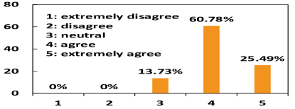
(a) Q1

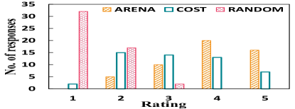
(b) Q2

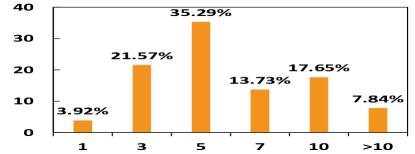
(c) Q4

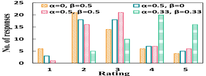
(d) Q5

(e) Q6

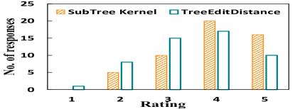
(f) Q7

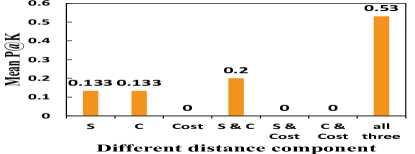
(g) b-tips

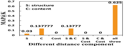
(h) i-tips

Figure 11: User study.

VIII-A User Study

We conducted a user study among cs undergraduate/postgraduate students who are enrolled in the database systems course in Xidian University. 51 unpaid volunteers participated in the study. Note that these volunteers are different from those who participated in the survey in Section II. After consenting to have their feedback recorded and analyzed, we presented a brief tutorial of the arena gui describing the tool and how to use it. Then they were allowed to explore it for an unstructured time. Through the gui, the participants can specify the choice of problem (b-tips vs i-tips), configure parameters (e.g., $\alpha,\beta,\lambda$), and switch between subtree kernel and tree edit distance.

US 1: Survey. We presented 30 predefined queries on IMDb to all volunteers. A list of returned alternative plans is shown to the participants for their feedback. For our study, we generate the alternative plans using arena, cost, and random. All these plans can be visualized using the arena gui. A participant can click on any returned alternative plan and arena will immediately plot it and the qep side-by-side, where the tree structure, physical operator of each node, as well as the estimated cost at each node are presented. Moreover, each different node representing different operator or same operator with different cost in an alternative plan is highlighted in red or green, respectively. Volunteers were allowed to take their own time to explore the alternative plan space. Finally, they were asked to fill up a survey form, which consists of a series of questions. Where applicable, every subject is asked to give a rating in the Likert scale of 1-5 with higher rating indicating greater agreement to the affirmative response to the question or the technique/setting. We also instructed them that there is no correlation between the survey outcome and their grades. In the following, we report the key results.

Q1: Does arena facilitate understanding of the qep selection process? Fig. 11a plots the results of the corresponding responses. Observe that 44 participants agree that the alternative plans returned by arena facilitate their understanding.

Q2: How well does arena/random/cost help in understanding the alternative plan space? In order to mitigate bias, the results of arena, cost, and random are presented in random order and participants were not informed of the approach used to select alternative plans. Fig. 11b reports the results. In general, arena receives the best scores (i.e., 36 out of 51 give a score over 3).

Q3: Preference for i-tips or b-tips. Among all the participants, 38 of them prefer to use b-tips whereas the remaining 13 prefer to use i-tips. The results justify that both these modes should be part of arena as different learners may prefer different mode for exploring alternative query plans.

Q4: How many alternative plans is sufficient to understand the qep selection? Fig. 11c shows the responses. Most participants think that 10 or less alternative plans are sufficient. Further feedbacks from these participants show that additional alternative plans exhibit limited marginal increase in their understanding. This also justifies that our approximate solution exhibits a diminishing return phenomenon.

Q5: Importance of structural, content, and cost differences. Fig. 11d reports the responses. Setting $\alpha$ (resp., $\beta$) as 0 indicates that the structural (resp., content) difference is not taken into account in arena. Similarly, by setting $\alpha=\beta=0.5$, arena ignores the cost difference between plans. We observe that $\alpha=\beta=1/3$ receives the best response. 36 participants give a score of 4 and above, while each of the remaining settings have less than 10 responses with scores 4-5. This highlights the importance of structural, content, and cost differences.

Q6: Importance of distance and relevance measures. $\lambda$ allows us to balance the impact of distance and relevance in selecting alternative plans. Fig. 11e reports the results. Clearly, by setting $\lambda=0.5$, the results of arena is significantly better than either disabling distance or relevance.

Q7: Tree Edit Distance vs Subtree Kernel. Fig. 11f reports the results. In general, subtree kernel-based structural difference computation strategy receives superior scores (i.e., 36 out of 51 give a score over 3) to tree edit distance-based strategies (i.e., 27 out 51). This justifies the choice of the former as the default structural difference computation technique in arena.

US 2: Impact of different distance components. We explore the impact of different distance components on alternative plan preferences. We consider various combinations of distance components ($x$ axis in Fig. 11(g) and 11(h)). For each combination, the distance components are of equal weight. These combinations were hidden from the learners to mitigate any bias. We choose 3 sql queries and ask the participants to mark and order the top-5 alternative plans (from 50 plans returned by arena under each settings) that they most want to see for each query. We then compare the user-marked list of plans in each case with the results returned by arena. For b-tips, we determine whether the returned result set contains the alternative plans that users expect to see and the number of such plans. We do not consider the order in which these plans appear. Therefore, we use the Mean P@k (k=5) [31] to measure similarity. i-tips, on the other hand, returns alternative plans iteratively. The order of appearance is an important factor here. Therefore, for i-tips, we use the MAP@K (k=5) [31].

The experimental results are reported in Fig. 11(g) and 11(h). Observe that regardless of the exploration mode, the effect when all the three distances (i.e., structural, content and cost) are considered at the same time is superior to other combinations. Interestingly, when the weight of cost distance is large, the values of Mean P@k and MAP@k are both 0, which means that the results that users expect to see cannot be obtained in this setting. That is, only considering the cost of plans as a factor for selecting alternative query plans will result in potentially sub-optimal collection as far as learners are concerned.

US 3: Result difference between i-tips and b-tips. Lastly, we investigate the differences in the returned results of the two proposed algorithms. We collected 80 groups of results from 20 volunteers, each of them is requested to use both i-tips and b-tips and view 10 aqps. Notably, in i-tips, for each returned aqp, users can mark whether it is useful to them and the aqps returned in the subsequent steps take this feedback into account. We observe that on average 56.07% of the returned aqps are different in both solutions.

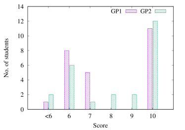
(a) Question 1

(b) Question 2

Figure 12: Score distribution in the quiz.

VIII-B Academic Outcomes

The preceding section demonstrates that volunteers find arena useful in understanding the qep selection process. In this section, we report the outcome of a quiz that test their understanding of this process. 50 learners from Xidian University participated in the quiz. These volunteers are different from those in the preceding section. They were given queries or query plans and were asked to answer questions on the followings: (a) other alternative plans that can also answer the query; (b) whether a plan is better than another; and (c) what plans the optimizer will never adopt. The questions can be found in appendix. In order to understand whether the adoption of arena useful to learners, we randomly separate them into a pair of test groups, each involving 25 students. The first group (referred to as GP1) does not have any experience with arena, but they were allowed to replay lecture video and review textbook material; and the second one (GP2) were exposed to arena before attending the quiz. Both groups are given the same time before the quiz, which are conducted simultaneously. The answer scripts of both groups were randomly mixed and graded by a teaching assistant, who is not involved with this research, in a double anonymity manner.

The distributions of scores for two questions in the quiz relevant to the study are depicted in Fig. 12. Observe that for both questions the performance of GP2 is significantly better than GP1. The average scores of learners in GP1 and GP2 are 7.76 and 8.24 for Question 1 (4.12 and 6.04 for Question 2), respectively. We also run a t-test for the assumption that the average score of GP2 is better in both questions. The $p$-values for the questions are 0.032 and 0.000303, respectively. In summary, GP2 significantly outperforms GP1 in the quiz.

Remark. We investigate the login and query logs of users since the system is open for public academic usage. The number of usage among the students in our University within recent two semesters are consistently above 100 until the holiday in each month. Among that, the learners have posed queries including nested subqueries, clustered functions, and multi-table (more than three table) joins. These facts demonstrate that learners actively turn to our system to improve their understanding of the process of plan exploration, especially for complex queries.

IX Related Work

Our work is related to the diversified top-k query, which aims to compute top-k results that are most relevant to a user query by taking diversity into consideration. This problem has been extensively studied in a wide variety of spectrum, such as, diversified keyword search in databases [46], documents [4] and graphs [14], diversified top-k pattern matchings [13], cliques [45] and structures [20] in a graph, and so on [47; 43]. In addition, [10] provides a comprehensive survey of different query result diversification approaches, [9] analyzed the complexity of query result diversification, and [15] used the axiomatic approach to analyze diversification systems. However, these techniques cannot be directly adopted here as they do not focus on informativeness of query plans in an rdbms.

Given the challenges faced by learners to learn sql [34], there has been increasing research efforts to build tools and techniques to facilitate comprehension of complex sql statements [23; 19; 32; 33; 26; 8]. There are also efforts to visualize sql queries [24; 26; 33] and query plans (e.g., [37]). However, scant attention has been paid to explore technologies that can enable learning of relational query processing [44; 29; 17; 6]. neuron [29] generates natural language descriptions of qeps using a rule-based technique and a question answering system to seek answers w.r.t. a qep. Using deep learning methods, lantern [44] enhances neuron to generate diversified natural language description of a qep. mocha [41] is a tool for learner-friendly interaction and visualization of the impact of alternative physical operator choices on a selected qep for a given sql query. In contrast to this work, mocha requires that the learner has clear preferences on the physical operators they wish to explore w.r.t. a qep. Picasso [17] depicts various visual diagrams of different qeps and their costs over the entire selectivity space. In summary, arena complements these efforts by facilitating exploration of informative aqps.

X Conclusions and Future Work

This paper presents a novel framework called arena that judiciously selects informative alternative query plans for an sql query in order to enhance one’s comprehension of the plan space considered by the underlying query optimizer during qep selection. To this end, arena implements efficient approximate algorithms that maximize the plan interestingness of the selected plans w.r.t. the qep or already-viewed plan set. A key use case of arena is for pedagogical support where it can facilitate comprehension of the query execution process in an off-the-shelf rdbms. Our performance study and user study with real-world learners indeed demonstrate the effectiveness of arena in facilitating comprehension of the alternative plan space. As part of future work, we plan to undertake a longitudinal study on the impact of arena on learners’ academic performance on this topic. Also, we wish to explore techniques to facilitate natural language-based interaction with the plan space.

[quiz questions]

-A Question 1

There is a SQL and the corresponding best plan (plan A) and an alternative plan (Plan B). Give some reasons why Plan A is better than Plan B. Explain each reason.

SELECTΨstudent.name
FROM Ψstudent, takes, course
WHERE   course.title = ’Image Processing’
        AND course.c_id = takes.c_id
        AND takes.year = 2002
        AND student.id = takes.id
        AND student.id < 1000;

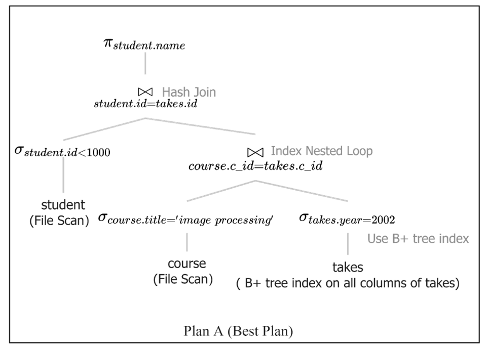
(a) Plan A

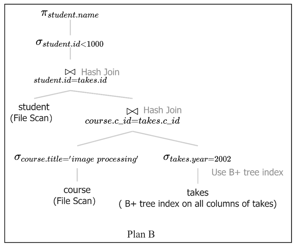
(b) Plan B

Figure 13: Best Plan and an alternative Plan.

-B Question 2

Consider the following SQL query that finds all courses offered by Professor Lembr in the spring.

SELECTΨtitle
FROM    course, teaches, instructor
WHEREΨcourse.c_id = teaches.c_id
        AND teaches.id = instructor.id
        AND instructor.name = ’Lembr’
        AND teaches.semester = ’Spring’;

TABLE III: Statistics of relations.

Relation	Cardinality	Number of pages	Primary key
course(c_id, title, credits)	20000	50	c_id
teaches (id, semester, c_id, year)	20000000	34000	(id, semester, c_id, year)
instructor (id, name)	5000	10	id

Assume that:

• teaches.id is a foreign key that references instructor.id.

• teaches.c_id is a foreign key that references course.c_id.

• teaches are evenly distributed on id and semester and semester can only be Spring or Fall.

• There is only one instructor named Lember.

• For each table, there is a B+ tree index on its primary key and all index pages are in memory.

• All intermediate tables can be stored in memory.

-B1 Question:

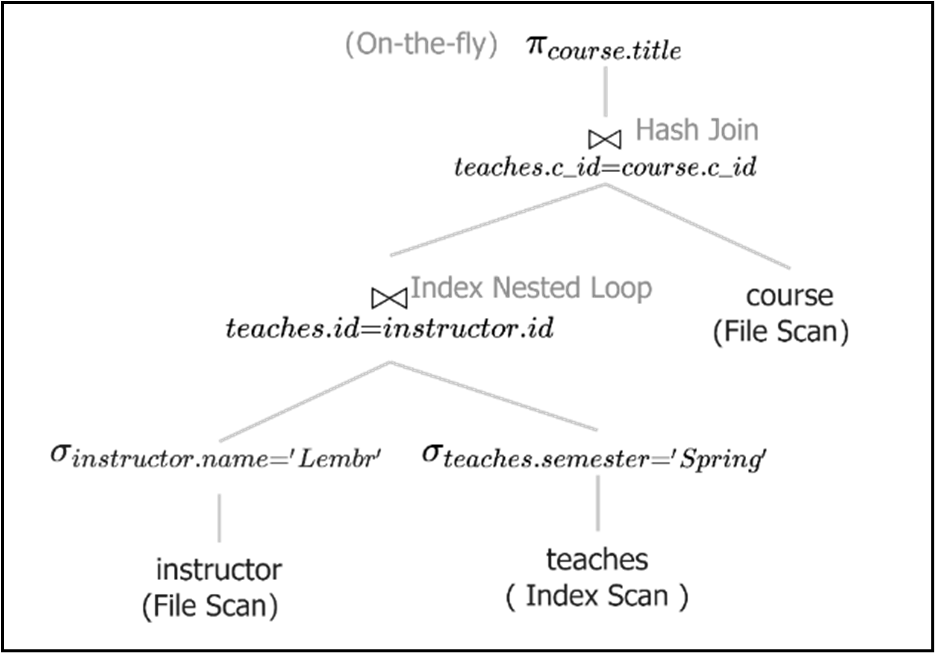
Figure 14: Physical plan

compute the worst cost of the physical query plan in Fig. 14.

-B2 Question:

Draw a query plan for the above query that the query optimizer will NOT consider. Justify your answer.

References

- [1]
- [2] Internet Movie Data Base (IMDb). http://www.imdb.com/.
- [3] TPC-H data set. http://www.tpc.org/tpch/.
- Angel and Koudas [2011] Albert Angel and Nick Koudas. 2011. Efficient diversity-aware search. In Proceedings of the ACM SIGMOD International Conference on Management of Data, SIGMOD 2011, Athens, Greece, June 12-16, 2011. ACM, 781–792.
- Arora et al. [2017] Sanjeev Arora and Yingyu Liang and Tengyu Ma. 2017. A Simple but Tough-to-Beat Baseline for Sentence Embeddings. In 5th International Conference on Learning Representations, ICLR 2017, Toulon, France, April 24-26, 2017, Conference Track Proceedings. OpenReview.net.
- [6] S. S. Bhowmick, H. Li. Towards Technology-Enabled Learning of Relational Query Processing. IEEE Data Engineering Bulletin, 45(3), 2022.
- [7] S. Chaudhuri. An Overview of Query Optimization in Relational Systems. In PODS, 1998.
- [8] J. Danaparamita, W. Gatterbauer. QueryViz: Helping Users Understand SQL Queries and Their Patterns. In EDBT, 2011.
- Deng and Fan [2013] Ting Deng and Wenfei Fan. 2013. On the Complexity of Query Result Diversification. Proc. VLDB Endow. 6, 8 (2013), 577–588.
- Drosou and Pitoura [2010] Marina Drosou and Evaggelia Pitoura. 2010. Search result diversification. ACM SIGMOD Record 39, 1 (2010), 41–47.
- Drosou and Pitoura [2012] Marina Drosou and Evaggelia Pitoura. 2012. DisC diversity: result diversification based on dissimilarity and coverage. Proc. VLDB Endow. 6, 1 (2012), 13–24.
- Drosou and Pitoura [2013] Marina Drosou and Evaggelia Pitoura. 2013. POIKILO: A Tool for Evaluating the Results of Diversification Models and Algorithms. Proc. VLDB Endow. 6, 12 (Aug. 2013), 1246–1249.
- Fan et al. [2013] Wenfei Fan, Xin Wang, and Yinghui Wu. 2013. Diversified Top-k Graph Pattern Matching. Proc. VLDB Endow. 6, 13 (2013), 1510–1521.
- Golenberg et al. [2008] Konstantin Golenberg, Benny Kimelfeld, and Yehoshua Sagiv. 2008. Keyword proximity search in complex data graphs. In Proceedings of the ACM SIGMOD International Conference on Management of Data, SIGMOD 2008, Vancouver, BC, Canada, June 10-12, 2008. ACM, 927–940.
- Gollapudi and Sharma [2009] Sreenivas Gollapudi and Aneesh Sharma. 2009. An Axiomatic Approach for Result Diversification. In Proceedings of the 18th International Conference on World Wide Web (Madrid, Spain) (WWW ’09). Association for Computing Machinery, 381–390.
- Graefe [1995] Goetz Graefe. 1995. The Cascades Framework for Query Optimization. IEEE Data Eng. Bull. 18, 3 (1995), 19–29.
- Haritsa [2010] Jayant R. Haritsa. 2010. The Picasso Database Query Optimizer Visualizer. Proc. VLDB Endow. 3, 2 (2010), 1517–1520.
- [18] S. Higgins, Z. M. Xiao, M. Katsipatak. The Impact of Digital Technology on Learning: A Summary for the Education. Education Endowment Foundation, 2012.
- [19] Y. Hu, Z. Miao, Z. Leong, H. Lim, Z. Zheng, S. Roy, K. Stephens-Martinez, J. Yang. I-Rex: An Interactive Relational Query Debugger for SQL. In ACM Technical Symposium on Computer Science Education (SIGCSE), 2022.
- Huang et al. [2013] Xin Huang, Hong Cheng, Rong-Hua Li, Lu Qin, and Jeffrey Xu Yu. 2013. Top-K Structural Diversity Search in Large Networks. Proc. VLDB Endow. 6, 13 (2013), 1618–1629.
- Ibaraki and Kameda [1984] Toshihide Ibaraki and Tiko Kameda. 1984. On the optimal nesting order for computing n-relational joins. ACM Transactions on Database Systems (TODS) 9, 3 (1984), 482–502.
- James et al. [2013] Gareth James, Daniela Witten, Trevor Hastie, and Robert Tibshirani. 2013. An introduction to statistical learning. Springer.
- [23] A. Kokkalis, P. Vagenas, A. Zervakis, A. Simitsis, G. Koutrika, Y. E. Ioannidis. Logos: A System for Translating Queries into Narratives. In SIGMOD, 2012.
- [24] W. Gatterbauer et al. Principles of Query Visualization. IEEE Data Engineering Bulletin, September 2022.
- Leis et al. [2015] Viktor Leis, Andrey Gubichev, Atanas Mirchev, Peter A. Boncz, Alfons Kemper, and Thomas Neumann. 2015. How Good Are Query Optimizers, Really? Proc. VLDB Endow. 9, 3 (2015), 204–215.
- [26] A. Leventidis, J. Zhang, C. Dunne, W. Gatterbauer, H. V. Jagadish, and M. Riedewald. QueryVis: Logic-based Diagrams help Users Understand Complicated SQL Queries Faster. In SIGMOD, 2020.
- Li and Liu [2007] Yujian Li and Bi Liu. 2007. A Normalized Levenshtein Distance Metric. IEEE Trans. Pattern Anal. Mach. Intell. 29, 6 (2007), 1091–1095.
- Li et al. [2016] Zhan Li, Olga Papaemmanouil, and Mitch Cherniack. 2016. OptMark: A Toolkit for Benchmarking Query Optimizers. In Proceedings of the 25th ACM International Conference on Information and Knowledge Management, CIKM 2016, Indianapolis, IN, USA, October 24-28, 2016. ACM, 2155–2160.
- Liu et al. [2019] Siyuan Liu, Sourav S Bhowmick, Wanlu Zhang, Shu Wang, Wanyi Huang, and Shafiq Joty. 2019. NEURON: Query Execution Plan Meets Natural Language Processing For Augmenting DB Education. In SIGMOD ’19: International Conference on Management of Data, Amsterdam, The Netherlands, June 30-July 5, 2019. ACM, 1953–1956.
- Marcus et al. [2021] Ryan Marcus, Parimarjan Negi, Hongzi Mao, Nesime Tatbul, Mohammad Alizadeh, and Tim Kraska. 2021. Bao: Making Learned Query Optimization Practical. In SIGMOD ’21: International Conference on Management of Data, Virtual Event, China, June 20-25, 2021. ACM, 1275–1288.
- McFee and Lanckriet [2010] Brian McFee and Gert RG Lanckriet. 2010. Metric learning to rank. In ICML.
- [32] Zhengjie Miao, Sudeepa Roy, Jun Yang. Explaining Wrong Queries Using Small Examples. SIGMOD, 2019.
- [33] D. Miedema, G. Fletcher. SQLVis: Visual Query Representations for Supporting SQL Learners. In VL/HCC, 2021.
- [34] D. Miedema, E. Aivaloglou, G. Fletcher. Identifying SQL Misconceptions of Novices: Findings from a Think-Aloud Study. In ICER, 2021.
- Pawlik and Augsten [2015] Mateusz Pawlik and Nikolaus Augsten. 2015. Efficient Computation of the Tree Edit Distance. ACM Trans. Database Syst. 40, 1, Article 3 (March 2015), 40 pages.
- Ravi et al. [2018] S. S. Ravi, Daniel J. Rosenkrantz, and Giri Kumar Tayi. 2018. Approximation Algorithms for Facility Dispersion. In Handbook of Approximation Algorithms and Metaheuristics, Second Edition, Volume 2: Contemporary and Emerging Applications. Chapman and Hall/CRC.
- [37] D. Scheibli, C. Dinse, A. Boehm. QE3D: Interactive Visualization and Exploration of Complex, Distributed Query Plans. In Proceedings of the 2015 ACM SIGMOD International Conference on Management of Data, 877-881, ACM, 2015.
- Shawe-Taylor and Cristianini [2004] John Shawe-Taylor and Nello Cristianini. 2004. Kernel Methods for Pattern Analysis. Cambridge University Press.
- Smola and Vishwanathan [2003] Alex Smola and S.v.n. Vishwanathan. 2003. Fast Kernels for String and Tree Matching. In Advances in Neural Information Processing Systems, Vol. 15.
- Soliman et al. [2014] Mohamed A. Soliman, Lyublena Antova, Venkatesh Raghavan, Amr El-Helw, Zhongxian Gu, Entong Shen, George C. Caragea, Carlos Garcia-Alvarado, Foyzur Rahman, Michalis Petropoulos, Florian Waas, Sivaramakrishnan Narayanan, Konstantinos Krikellas, and Rhonda Baldwin. 2014. Orca: a modular query optimizer architecture for big data. In International Conference on Management of Data, SIGMOD 2014, Snowbird, UT, USA, June 22-27, 2014. ACM, 337–348.
- [41] J. Tan, D. Yeo, R. Neoh, H.-E. Chua, S. S. Bhowmick. MOCHA: A Tool for Visualizing Impact of Operator Choices in Query Execution Plans for Database Education. PVLDB, 15(12), 2022.
- Waas and Galindo-Legaria [2000] Florian Waas and César A. Galindo-Legaria. 2000. Counting, Enumerating, and Sampling of Execution Plans in a Cost-Based Query Optimizer. In Proceedings of the 2000 ACM SIGMOD International Conference on Management of Data, May 16-18, 2000, Dallas, Texas, USA. ACM, 499–509.
- Wang et al. [2018] Bin Wang, Rui Zhu, Xiaochun Yang, and Guoren Wang. 2018. Top-K representative documents query over geo-textual data stream. World Wide Web 21, 2 (2018), 537–555.
- Wang et al. [2021] Weiguo Wang, Sourav S. Bhowmick, Hui Li, Shafiq R. Joty, Siyuan Liu, and Peng Chen. 2021. Towards Enhancing Database Education: Natural Language Generation Meets Query Execution Plans. In SIGMOD ’21: International Conference on Management of Data, Virtual Event, China, June 20-25, 2021. ACM, 1933–1945.
- Yuan et al. [2015] Long Yuan, Lu Qin, Xuemin Lin, Lijun Chang, and Wenjie Zhang. 2015. Diversified top-k clique search. In 31st IEEE International Conference on Data Engineering, ICDE 2015, Seoul, South Korea, April 13-17, 2015. IEEE Computer Society, 387–398.
- Zhao et al. [2011] Feng Zhao, Xiaolong Zhang, Anthony KH Tung, and Gang Chen. 2011. Broad: Diversified keyword search in databases. Technical Report.
- Zhu et al. [2017] Rui Zhu, Bin Wang, Xiaochun Yang, Baihua Zheng, and Guoren Wang. 2017. SAP: Improving Continuous Top-K Queries Over Streaming Data. IEEE Trans. Knowl. Data Eng. 29, 6 (2017), 1310–1328.