Structure-based Drug Design with Equivariant Diffusion Models

Abstract

Structure-based drug design (SBDD) aims to design small-molecule ligands that bind with high affinity and specificity to pre-determined protein targets. In this paper, we formulate SBDD as a 3D-conditional generation problem and present DiffSBDD, an SE(3)-equivariant 3D-conditional diffusion model that generates novel ligands conditioned on protein pockets. Comprehensive in silico experiments demonstrate the efficiency and effectiveness of DiffSBDD in generating novel and diverse drug-like ligands with competitive docking scores. We further explore the flexibility of the diffusion framework for a broader range of tasks in drug design campaigns, such as off-the-shelf property optimization and partial molecular design with inpainting.

1 Introduction

The rational design of molecular drug-like compounds remains an outstanding challenge in biopharmaceutical research. Structure-based drug design (SBDD) aims to generate small-molecule ligands that bind to a specific 3D protein structure with high affinity and specificity (Anderson, 2003). Traditionally, SBDD campaingns are initiated either by high-throughput experimental or virtual screening (Lyne, 2002; Shoichet, 2004) of large chemical databases. Not only is this expensive and time consuming but it restricts the exploration of chemical space to the historical knowledge of previously studied molecules, with a further emphasis usually placed on commercial availability (Irwin & Shoichet, 2005). Moreover, the optimization of initial lead molecules is often a biased process, with significant reliance on human intuition (Ferreira et al., 2015).

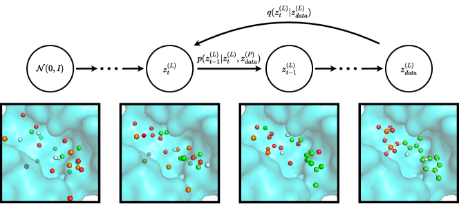
Figure 1: DiffSBDD in the protein-conditioned scenario. We first simulate the forward diffusion process $q$ to gain a trajectory of progressively noised samples over $T$ timesteps. We then train a model $p_{\theta}$ conditional on the target structure to reverse or denoise this process. Once trained, we can sample new drug candidates from a Gaussian distribution $\mathcal{N}\left(\boldsymbol{0},\boldsymbol{I}\right)$. Both atom features and coordinates are diffused throughout the process. Ligands ($z^{(L)}$) are represented as fully-connected graphs during the diffusion process (edges not shown for clarity) and covalent bonds are added to the resultant point cloud at the end of generation. The protein ($z^{(P)}$) is represented as a graph but is shown as a surface here for clarity.

Recent advances in geometric deep learning, especially in modelling geometric structures of biomolecules (Bronstein et al., 2021; Atz et al., 2021), provide a promising direction for structure-based drug design (Gaudelet et al., 2021). Despite remarkable progress in the use of deep learning as surrogate docking models (Lu et al., 2022; Stärk et al., 2022; Corso et al., 2022), deep learning-based design of ligands that bind to target proteins remains an open problem. Early attempts have been made to represent molecules as atomic density maps, and variational auto-encoders were utilized to generate new atomic density maps corresponding to novel molecules (Ragoza et al., 2022). However, it is nontrivial to map atomic density maps back to molecules, necessitating a subsequent atom-fitting stage. Follow-up work addressed this limitation by representing molecules as 3D graphs with atomic coordinates and types which circumvents the post-processing steps.  Li et al. (2021) proposed an autoregressive generative model to sample ligands given the protein pocket as a conditioning constraint.  Peng et al. (2022) improved this method by using an $E(3)$-equivariant graph neural network which respects rotation and translation symmetries in 3D space. Similarly, Drotár et al. (2021); Liu et al. (2022) used autoregressive models to generate atoms sequentially and incorporate angles during the generation process.  Li et al. (2021) formulated the generation process as a reinforcement learning problem and connected the generator with Monte Carlo Tree Search for protein pocket-conditioned ligand generation. However, the main premise of sequential generation methods may not hold in real scenarios, since it imposes an artificial ordering scheme in the generation process and, as a result, the global context of the generated ligands may be lost. In addition, previous methods often focus on de novo ligand generation and are not readily applicable to other drug design tasks and downstream molecular optimization.

In this work, we propose an $SE(3)$-equivariant 3D-conditional diffusion model for SBDD (DiffSBDD) that respects translation, rotation, and permutation symmetries. We evaluate our model in the following ways:

• We benchmark our model on the de novo molecule generation task, for which we introduce two strategies, protein-conditioned generation, which considers the protein as a fixed context, and learning the joint distribution of protein and ligand atoms. In the latter case, conditional samples can be produced with a modified sampling scheme.

• We further demonstrate how pre-trained DiffSBDD models can be used out-of-the-box to optimize arbitary molecular properties via a noise/denoise scheme in combination with an evolutionary algorithm.

• We present an inpainting-inspired approach to accomplish challenging molecular (re)design problems, such as scaffold hopping/elaboration and fragment growing/merging, all training a new model.

Finally, we curate an experimentally determined binding dataset derived from Binding MOAD (Hu et al., 2005), which supplements the commonly used synthetic CrossDocked (Francoeur et al., 2020) dataset to validate our model performance under realistic binding scenarios. The experimental results demonstrate that DiffSBDD is capable of generating novel, diverse and drug-like ligands with high predicted binding affinities to given protein pockets, and case studies underline the method’s flexibility as a tool for candidate molecule refinement.

2 Background

Denoising Diffusion Probabilistic Models

Denoising diffusion probabilistic models (DDPMs) (Sohl-Dickstein et al., 2015; Ho et al., 2020) are a class of generative models inspired by non-equilibrium thermodynamics. Briefly, they define a Markovian chain of random diffusion steps by slowly adding noise to sample data and then learning the reverse of this process (typically via a neural network) to reconstruct data samples from noise.

In this work, we closely follow the framework developed by Hoogeboom et al. (2022). In our setting, data samples are atomic point clouds $\bm{z}_{\text{data}}=[\bm{x},\bm{h}]$ with 3D geometric coordinates $\bm{x}\in\mathbb{R}^{N\times 3}$ and categorical features $\bm{h}\in\mathbb{R}^{N\times d}$, where $N$ is the number of atoms. A fixed noise process

$$q(\bm{z}_{t}|\bm{z}_{\text{data}})=\mathcal{N}(\bm{z}_{t}|\alpha_{t}\bm{z}_{\text{data}},\sigma_{t}^{2}\bm{I})$$ (1)

adds noise to the data $\bm{z}_{\text{data}}$ and produces a latent noised representation $\bm{z}_{t}$ for $t=0,\dotsc,T$. $\alpha_{t}$ controls the signal-to-noise ratio $\text{SNR}(t)=\alpha_{t}^{2}/\sigma_{t}^{2}$ and follows either a learned or pre-defined schedule from $\alpha_{0}\approx 1$ to $\alpha_{T}\approx 0$ (Kingma et al., 2021). We also choose a variance-preserving noising process (Song et al., 2020) with $\alpha_{t}=\sqrt{1-\sigma_{t}^{2}}$.

Since the noising process is Markovian, we can write the denoising transition from time step $t$ to $s<t$ in closed form as

$$q(\bm{z_{s}}|\bm{z}_{\text{data}},\bm{z}_{t})=\mathcal{N}\Big{(}\bm{z}_{s}\big{|}\frac{\alpha_{t|s}\sigma_{s}^{2}}{\sigma_{t}^{2}}\bm{z}_{t}+\frac{\alpha_{s}\sigma_{t|s}^{2}}{\sigma_{t}^{2}}\bm{z}_{\text{data}},\frac{\sigma_{t|s}^{2}\sigma_{s}^{2}}{\sigma_{t}^{2}}\bm{I}\Big{)}$$ (2)

with $\alpha_{t|s}=\frac{\alpha_{t}}{\alpha_{s}}$ and $\sigma_{t|s}^{2}=\sigma_{t}^{2}-\alpha_{t|s}^{2}\sigma_{s}^{2}$ following the notation of Hoogeboom et al. (2022). This true denoising process depends on the data sample $\bm{z}_{\text{data}}$, which is not available when using the model for generating new samples. Instead, a neural network $\phi_{\theta}$ is used to approximate the sample $\hat{\bm{z}}_{\text{data}}$. More specifically, we can reparameterize Equation (1) as $\bm{z}_{t}=\alpha_{t}\bm{z}_{\text{data}}+\sigma_{t}\bm{\epsilon}$ with $\bm{\epsilon}\sim\mathcal{N}(\bm{0},\bm{I})$ and directly predict the Gaussian noise $\hat{\bm{\epsilon}}_{\theta}=\phi_{\theta}(\bm{z}_{t},t)$. Thus, $\hat{\bm{z}}_{\text{data}}$ is simply given as $\hat{\bm{z}}_{\text{data}}=\frac{1}{\alpha_{t}}\bm{z}_{t}-\frac{\sigma_{t}}{\alpha_{t}}\hat{\bm{\epsilon}}_{\theta}$.

The neural network is trained to maximise the likelihood of observed data by optimizing a variational lower bound on the data, which is equivalent to the simplified training objective (Ho et al., 2020; Kingma et al., 2021) $\mathcal{L}_{\text{train}}=\frac{1}{2}||\bm{\epsilon}-\phi_{\theta}(\bm{z}_{t},t)||^{2}$ up to a scale factor (see Appendix A for details).

$E(n)$-equivariant Graph Neural Networks

A function $f:\mathcal{X}\rightarrow\mathcal{Y}$ is said to be equivariant w.r.t. the group $G$ if $f(g.\boldsymbol{x})=g.f(\boldsymbol{x})$, where $g.$ denotes the action of the group element $g\in G$ on $\mathcal{X}$ and $\mathcal{Y}$ (Serre et al., 1977). Graph Neural Networks (GNNs) are learnable functions that process graph-structured data in a permutation-equivariant way, making them particularly useful for molecular systems where nodes do not have an intrinsic order. Permutation invariance means that $\mathrm{GNN}(\boldsymbol{\Pi}\mathbf{X})=\boldsymbol{\Pi}\,\mathrm{GNN}(\mathbf{X})$ where $\boldsymbol{\Pi}$ is an $n\times n$ permutation matrix acting on the node feature matrix. Since the nodes of the molecular graph represent the 3D coordinates of atoms, we are interested in additional equivariance w.r.t. the Euclidean group $E(3)$ or rigid transformations. An $E(3)$-equivariant GNN (EGNN) satisfies $\mathrm{EGNN}(\boldsymbol{\Pi}\mathbf{X}\mathbf{A}+\mathbf{b})=\boldsymbol{\Pi}\,\mathrm{EGNN}(\mathbf{X})\mathbf{A}+\mathbf{b}$ for an orthogonal $3\times 3$ matrix $\mathbf{A}^{\top}\mathbf{A}=\mathbf{I}$ and some translation vector $\mathbf{b}$ added row-wise.

In our case, since the nodes have both geometric atomic coordinates $\boldsymbol{x}$ as well as atomic type features $\boldsymbol{h}$, we can use a simple implementation of EGNN proposed by Satorras et al. (2021), in which the updates for features $\bm{h}$ and coordinates $\bm{x}$ of node $i$ at layer $l$ are computed as follows:

$$\boldsymbol{m}_{ij} =\phi_{e}(\boldsymbol{h}^{l}_{i},\boldsymbol{h}^{l}_{j},d_{ij}^{2},a_{ij}),~{}\tilde{e}_{ij}=\phi_{\text{att}}(\bm{m}_{ij})$$ (3)

$$\boldsymbol{h}_{i}^{l+1} =\phi_{h}(\boldsymbol{h}^{l}_{i},\sum_{j\neq i}\tilde{e}_{ij}\boldsymbol{m}_{ij})$$ (4)

$$\boldsymbol{x}_{i}^{l+1} =\boldsymbol{x}_{i}^{l}+\sum_{j\neq i}\frac{\boldsymbol{x}_{i}^{l}-\boldsymbol{x}_{j}^{l}}{d_{ij}+1}\phi_{x}(\boldsymbol{h}^{l}_{i},\boldsymbol{h}^{l}_{j},d_{ij}^{2},a_{ij})$$ (5)

where $\phi_{e}$, $\phi_{\text{att}}$, $\phi_{h}$ and $\phi_{h}$ are learnable Multi-layer Perceptrons (MLPs) and $d_{ij}$ and $a_{ij}$ are the relative distances and edge features between nodes $i$ and $j$ respectively. In Section 3.1, we propose a modified coordinate update that breaks symmetry to reflections.

3 Equivariant Diffusion Models for SBDD

We use an equivariant DDPM to generate molecules and binding conformations jointly with respect to a specific protein target. We represent protein and ligand point clouds as graphs that are further processed by EGNNs (Satorras et al., 2021). We consider two distinct approaches to 3D pocket conditioning: (1) a conditional DDPM that receives a fixed pocket representation as context in each denoising step, and (2) a model that is trained to approximate the joint distribution of ligand-pocket pairs combined with a modified sampling procedure at inference time.

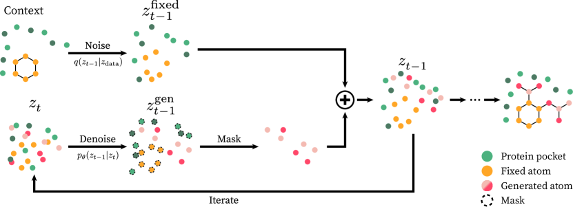
Figure 2: Replacement method for molecule inpainting. Sampling is conditioned on the fixed part of the molecular system by combining a forward diffused version of the corresponding atoms $z_{t-1}^{\text{fixed}}$ with the current generated representation $z_{t-1}^{\text{gen}}$ in each denoising step. Pocket nodes are shown in green hues.

3.1 Pocket-conditioned small molecule generation

In the conditional molecule generation setup, we provide fixed three-dimensional context in each step of the denoising process. To this end, we supplement the ligand node point cloud $\bm{z}^{(L)}_{t}$, denoted by superscript $L$, with protein pocket nodes $\bm{z}^{(P)}_{\text{data}}$, denoted by superscript $P$, that remain unchanged throughout the reverse diffusion process (Figure 1).

We parameterize the noise predictor $\hat{\bm{\epsilon}}_{\theta}=\phi_{\theta}(\bm{z}^{(L)}_{t},\bm{z}^{(P)}_{\text{data}},t)$ with an EGNN (Satorras et al., 2021; Hoogeboom et al., 2022). To process ligand and pocket nodes with a single GNN, atom types and residue types are first embedded in a joint node embedding space by separate learnable MLPs. We employ the same message-passing scheme outlined in Equations (3)-(5), however, following (Igashov et al., 2022), we do not update the coordinates of nodes that belong to the pocket to ensure the three-dimensional protein context remains fixed throughout the EGNN layers.

Equivariance

In the probabilistic setting with 3D-conditioning, we would like to ensure $SE(3)$-equivariance in the following sense: evaluating the likelihood of a molecule $\bm{x}^{(L)}\in\mathbb{R}^{3\times N_{L}}$ given the three-dimensional representation of a protein pocket $\bm{x}^{(P)}\in\mathbb{R}^{3\times N_{P}}$ should not depend on global $SE(3)$-transformations of the system, i.e. $p(\bm{R}\bm{x}^{(L)}+\bm{t}|\bm{R}\bm{x}^{(P)}+\bm{t})=p(\bm{x}^{(L)}|\bm{x}^{(P)})$ for orthogonal $\bm{R}\in\mathbb{R}^{3\times 3}$ with $\bm{R}^{T}\bm{R}=\bm{I}$, $\det(\bm{R})=1$ and $\bm{t}\in\mathbb{R}^{3}$ added column-wise. At the same time, it should be possible to generate samples $\bm{x}^{(L)}\sim p(\bm{x}^{(L)}|\bm{x}^{(P)})$ from this conditional probability distribution so that equivalently transformed ligands $\bm{R}\bm{x}^{(L)}+\bm{t}$ are sampled with the same probability if the input pocket is rotated and translated and we sample from $p(\bm{R}\bm{x}^{(L)}+\bm{t}|\bm{R}\bm{x}^{(P)}+\bm{t})$. This definition explicitly excludes reflections which are connected with chirality and can alter a biomolecule’s properties.

Equivariance to the orthogonal group $O(3)$ (comprising rotations and reflections) is achieved because we model both prior and transition probabilities with isotropic Gaussians where the mean vector transforms equivariantly w.r.t. rotations of the context (see  Hoogeboom et al. (2022) and Appendix E). Ensuring translation equivariance, however, is not as easy because the transition probabilities $p(\bm{z}_{t-1}|\bm{z}_{t})$ are not inherently translation-equivariant. In order to circumvent this issue, we follow previous works (Köhler et al., 2020; Xu et al., 2022; Hoogeboom et al., 2022) by limiting the whole sampling process to a linear subspace where the center of mass (CoM) of the system is zero. In practice, this is achieved by subtracting the center of mass of the system before performing likelihood computations or denoising steps. Since equivariance of the transition probabilities depends on the parameterization of the noise predictor $\hat{\bm{\epsilon}}_{\theta}$, we can make the model sensitive to reflections with a simple additive term in the EGNN’s coordinate update:

$$\bm{x}_{i}^{l+1}=\bm{x}_{i}^{l}+\sum_{j\neq i}\frac{\bm{x}_{i}^{l}-\bm{x}_{j}^{l}}{d_{ij}+1}\phi_{x}^{d}(\bm{h}^{l}_{i},\bm{h}^{l}_{j},d_{ij}^{2},a_{ij})+\\ \frac{(\bm{x}_{i}^{l}-\bar{\bm{x}}^{l})\times(\bm{x}_{j}^{l}-\bar{\bm{x}}^{l})}{||(\bm{x}_{i}^{l}-\bar{\bm{x}}^{l})\times(\bm{x}_{j}^{l}-\bar{\bm{x}}^{l})||+1}\phi_{x}^{\times}(\bm{h}^{l}_{i},\bm{h}^{l}_{j},d_{ij}^{2},a_{ij}),$$ (6)

using the cross product which changes sign under reflection. Here, $\bar{\bm{x}}^{l}$ denotes the center of mass of all nodes at layer $l$. $\phi_{x}^{\times}$ is an additional MLP. This modification is discussed in more detail in Appendix F.

3.2 Joint generation of pocket and small molecule

In addition to the pocket-conditional model presented above, we also train a DDPM for generating molecular systems consisting of pocket atoms and ligand atoms. This unconditional model thus approximates the joint distribution $p(\bm{z}^{(L)}_{\text{data}},\bm{z}^{(P)}_{\text{data}})$. The training procedure is identical to the equivariant molecule generation procedure developed by Hoogeboom et al. (2022) aside from the fully-connected neural networks that embed protein and ligand node features in a common space as described in Section 3.1, and the breaking of reflection symmetry using Equation (6).

When combined with inpainting, as described in the following section, this model can be used for target-specific molecule generation. Here, we do not learn the conditional distribution during training but delegate conditioning entirely to the sampling algorithm.

3.3 Inpainting

Generating compounds or parts thereof conditioned on the molecular context is reminiscent of inpainting, a technique originally introduced for completing missing parts of images (Song et al., 2020; Lugmayr et al., 2022) but also adopted in other domains, including biomolecular structures (Wang et al., 2022). An unconditional diffusion model can generate approximate conditional samples if the given context is injected into the sampling process by modifying the probabilistic transition steps. This idea has been successfully applied to image imputation (Song et al., 2020; Lugmayr et al., 2022) but can be readily extended to three-dimensional point cloud data.

As an example, Figure 2 outlines the sampling procedure for molecule generation with a fixed scaffold. A subset of all atoms is fixed and serves as the molecular context we want to condition on. All other atoms are generated by the DDPM. To the this end, we diffuse the fixed atoms at each time step and predict a new latent representation $z_{t-1}^{\text{gen}}$ with the neural network. We then replace the generated atoms corresponding to fixed nodes with their forward noised counterparts:

$$\bm{z}_{t-1}^{\text{fixed}} \sim q(\bm{z}_{t-1}|\bm{z}_{\text{data}})$$ (7)

$$\bm{z}_{t-1}^{\text{gen}} \sim p_{\theta}(\bm{z}_{t-1}|\bm{z}_{t})$$ (8)

$$\bm{z}_{t-1} =\big{[}\bm{z}_{t-1}^{\text{fixed}},\bm{z}_{t-1,i\notin\mathcal{M}}^{\text{gen}}\big{]},$$ (9)

where $\mathcal{M}$ denotes the set of mask indices used to uniquely identify nodes corresponding to fixed atoms. In this manner, we traverse the Markov chain in reverse order from $t=T$ to $t=0$ to generate conditional samples. Because the noise schedule decreases the noising process’s variance to almost zero at $t=0$ (Equation (1)), the final sample is guaranteed to contain an unperturbed representation of the fixed atoms. This approach can be applied to pocket-conditioned ligand-inpainting by fixing all pocket nodes when sampling from the joint distribution model (Section 3.2). However, it is much more general and allows us to mask and replace arbitrary parts of the ligand-pocket system without retraining—an option we explore in Section 4.4.

Equivariance

Since the equivariant diffusion process is defined for a CoM-free system, we must ensure that this requirement remains satisfied after the substitution step in Equation (9). To prevent a CoM shift, we therefore translate the fixed atom representation so that its center of mass coincides with the predicted representation: $\tilde{\bm{x}}_{t-1}^{\text{fixed}}=\bm{x}_{t-1}^{\text{fixed}}+\frac{1}{n}\sum_{i\in\mathcal{M}}\bm{x}_{t-1,i}^{\text{gen}}-\frac{1}{n}\sum_{i\in\mathcal{M}}\bm{x}_{t-1,i}^{\text{fixed}}$ before creating the new combined representation $\bm{z}_{t-1}=[\tilde{\bm{z}}_{t-1}^{\text{fixed}},\bm{z}_{t-1,i\notin\mathcal{M}}^{\text{gen}}]$ with $\tilde{\bm{z}}_{t-1}^{\text{fixed}}=[\tilde{\bm{x}}_{t-1}^{\text{fixed}},\bm{h}_{t-1}^{\text{fixed}}]$ and $n=|\mathcal{M}|$.

Resampling

Trippe et al. (2022) show that this simple replacement method inevitably introduces approximation error that can lead to inconsistent inpainted regions. In our experiments, we observe that the inpainting solution sometimes generates dislocated molecules that are not properly positioned in the target pocket (see Figure 7 for an example). Trippe et al. (2022) propose to address this limitation with a particle filtering scheme that upweights more consistent samples in each denoising step. We, however, choose to adopt the conceptually simpler idea of resampling (Lugmayr et al., 2022), where each latent representation is repeatedly diffused back and forth before advancing to the next time step as reviewed in Appendix C.1. This enables the model to harmonize its prediction for the generated part and the noisy sample from the fixed part (Eq. (7)), which does not include any information about the generated part. We choose $r=10$ resamplings per denoising step based on empirical results discussed in Appendix C.1.

4 Experiments

4.1 Setup

Datasets

We use the CrossDocked dataset (Francoeur et al., 2020) and follow the same filtering and splitting strategies as in previous work (Luo et al., 2021; Peng et al., 2022). This results in 100,000 high-quality protein-ligand pairs for the training set and 100 proteins for the test set. The split is done by 30% sequence identity using MMseqs2 (Steinegger & Söding, 2017).

Binding MOAD

We also evaluate our method on experimentally determined protein-ligand complexes found in Binding MOAD (Hu et al., 2005) which are filtered and split based on the proteins’ enzyme commission number as described in Appendix D. This results in 40,344 protein-ligand pairs for training and 130 pairs for testing.

Figure 3: Example molecules generated by DiffSBDD. Top row: DiffSBDD-inpainted trained on the CrossDocked dataset evaluated against the targets PDB: 4tos and PDB: 2v3r. Bottom row: DiffSBDD-conditional trained on the Binding MOAD dataset evaluated against the targets PDB: 6c0b and PDB: 3gt9. ‘Sim’ is the Tanimoto similarity between the generated and reference ligand.

Baselines

We compare with three recent deep learning methods for structure-based drug design. 3D-SBDD (Luo et al., 2021), Pocket2Mol (Peng et al., 2022) and GraphBP (Liu et al., 2022) are auto-regressive schemes relying on graph representations of the protein pocket and previously placed atoms to predict probabilities based on which new atoms are added. 3D-SBDD uses heuristics to infer bonds from generated atomic point clouds while Pocket2Mol directly predicts them during the sequential generation process. GraphBP incorporates relative locations with respect to a local coordinate system when placing each new atom. Additionally, we include a concurrently developed diffusion model for target-aware molecule design, TargetDiff (Guan et al., 2023), in the comparison. TargetDiff is conceptually very similar to our conditionally trained model (DiffSBDD-cond) but employs a different diffusion formalism for the categorical atom types. For 3D-SBDD, Pocket2Mol and TargetDiff, we re-evaluate the generated ligands on the CrossDocked dataset from the original papers. For GraphBP, we train the model with both CrossDocked and Binding MOAD datasets with the default hyperparameters. We also attempted to train Pocket2Mol on Binding MOAD, but did not manage to robustly train the model on this dataset due to instability during training.

Evaluation

For every experiment, we evaluated all combinations of all-atom and $C_{\alpha}$ level graphs with conditional and inpainting-based approaches respectively. Full details of model architecture and hyperparameters are given in Appendix C. We sampled 100 valid molecules for each target pocket and removed all atoms that are not bonded to the largest connected fragment. Ligand sizes were sampled from the training distribution as described in Appendix C. This procedure yields significantly smaller molecules than the reference ligands from the test set. We therefore increase the mean ligand size by 5 atoms for CrossDocked and 10 atoms for Binding MOAD, respectively, to sample approximately equally sized molecules. This correction improves the observed docking scores which are highly correlated with the ligand size (see Figure 6).

We employ widely-used metrics to assess the quality of our generated molecules (Peng et al., 2022; Li et al., 2021): (1) Vina Score is an empirical estimation of binding affinity between small molecules and their target pocket; (2) QED is a simple quantitative estimation of drug-likeness combining several desirable molecular properties; (3) SA (synthetic accessibility) is a measure estimating the difficulty of synthesis; (4) Lipinski measures how many rules in the Lipinski rule of five (Lipinski et al., 2012), which is a loose rule of thumb to assess the drug-likeness of molecules, are satisfied; (5) Diversity is computed as the average pairwise dissimilarity (1 - Tanimoto similarity) between all generated molecules for each pocket; (6) Inference Time is the average time to sample 100 molecules for one pocket across all targets. All docking scores and chemical properties are calculated with QuickVina2 (Alhossary et al., 2015) and RDKit (Landrum et al., 2016).

4.2 De novo molecular design

Table 1: Evaluation of generated molecules for targets from the CrossDocked and Binding MOAD test sets. The first, second, and third best performance are highlighted in each column. ^∗ denotes that we re-evaluate the generated ligands provided by the authors. The inference times are taken from their papers.

Vina (All) ($\downarrow$) Vina (Top-10%) ($\downarrow$) QED ($\uparrow$) SA ($\uparrow$) Lipinski ($\uparrow$) Diversity ($\uparrow$) Time (s, $\downarrow$) CrossDocked Test set $-6.871\pm 2.32$ — $0.476\pm 0.20$ $0.728\pm 0.14$ $4.340\pm 1.14$ — — 3D-SBDD (Luo et al., 2021)^∗ $-5.888\pm 1.91$ $-7.289\pm 2.34$ gray!10 $0.502\pm 0.17$ gray!10 $0.675\pm 0.14$ gray!10 $4.787\pm 0.51$ gray!10 $0.742\pm 0.09$ $19659\pm 14704$ Pocket2Mol (Peng et al., 2022)^∗ $-7.058\pm 2.80$ $-8.712\pm 3.18$ gray!30 $0.572\pm 0.16$ gray!30 $0.752\pm 0.12$ gray!30 $4.936\pm 0.27$ $0.735\pm 0.15$ $2504\pm 2207$ GraphBP (Liu et al., 2022) $-4.719\pm 4.03$ $-7.165\pm 1.40$ gray!10 $0.502\pm 0.12$ $0.307\pm 0.09$ gray!22 $4.883\pm 0.37$ gray!30 $0.844\pm 0.01$ gray!30 $10.247\pm 1.08$ TargetDiff (Guan et al., 2023)^∗ gray!22 $-7.318\pm 2.47$ gray!22 $-9.669\pm 2.55$ $0.483\pm 0.20$ $0.584\pm 0.13$ $4.594\pm 0.83$ $0.718\pm 0.09$ $\sim 3428$ DiffSBDD-cond ($C_{\alpha}$) $-6.770\pm 2.73$ $-8.796\pm 1.75$ $0.475\pm 0.22$ $0.612\pm 0.12$ $4.536\pm 0.91$ $0.725\pm 0.06$ gray!22 $49.651\pm 17.34$ DiffSBDD-inpaint ($C_{\alpha}$) gray!10 $-7.177\pm 3.28$ gray!10 $-9.233\pm 1.82$ gray!22 $0.556\pm 0.20$ gray!22 $0.729\pm 0.12$ $4.742\pm 0.59$ $0.718\pm 0.07$ gray!10 $94.481\pm 38.86$ DiffSBDD-cond $-6.950\pm 2.06$ $-9.120\pm 2.16$ $0.469\pm 0.21$ $0.578\pm 0.13$ $4.562\pm 0.89$ $0.728\pm 0.07$ $135.866\pm 51.66$ DiffSBDD-inpaint gray!30 $-7.333\pm 2.56$ gray!30 $-9.927\pm 2.59$ $0.467\pm 0.18$ $0.554\pm 0.12$ $4.702\pm 0.64$ gray!22 $0.758\pm 0.05$ $160.314\pm 73.30$ Binding MOAD Test set $-8.412\pm 2.03$ — $0.522\pm 0.17$ $0.692\pm 0.12$ $4.669\pm 0.49$ — — GraphBP (Liu et al., 2022) $-4.843\pm 2.24$ $-6.629\pm 0.95$ gray!10 $0.512\pm 0.11$ $0.310\pm 0.09$ gray!30 $4.945\pm 0.27$ gray!30 $0.826\pm 0.01$ gray!30 $13.761\pm 1.55$ DiffSBDD-cond ($C_{\alpha}$) $-6.863\pm 1.59$ $-8.587\pm 1.34$ $0.480\pm 0.20$ $0.554\pm 0.11$ $4.662\pm 0.68$ gray!10 $0.714\pm 0.05$ gray!22 $36.285\pm 8.13$ DiffSBDD-inpaint ($C_{\alpha}$) gray!10 $-6.926\pm 3.39$ gray!10 $-9.124\pm 1.35$ gray!30 $0.548\pm 0.19$ gray!22 $0.580\pm 0.13$ gray!10 $4.757\pm 0.51$ $0.709\pm 0.05$ gray!10 $58.305\pm 17.35$ DiffSBDD-cond gray!22 $-7.171\pm 1.89$ gray!22 $-9.184\pm 2.23$ $0.436\pm 0.20$ gray!10 $0.568\pm 0.12$ $4.542\pm 0.79$ gray!10 $0.714\pm 0.08$ $336.061\pm 85.02$ DiffSBDD-inpaint gray!30 $-7.309\pm 4.03$ gray!30 $-9.840\pm 2.18$ gray!22 $0.542\pm 0.21$ gray!30 $0.615\pm 0.12$ gray!22 $4.777\pm 0.53$ gray!22 $0.739\pm 0.05$ $369.873\pm 124.54$

De novo molecular design refers to designing new molecules from scratch. In our context, we sample new ligands that bind to specific protein pockets. We present quantitative benchmarks covering a range of molecular properties and in silico docking scores (Table 1) and provide examples of generated molecules for a qualitative assessment (Figure 3).

CrossDocked

Overall, the experimental results in Table 1 suggest that DiffSBDD can generate diverse small-molecule compounds with predicted high binding affinity, outperforming state-of-the-art methods. DiffSBDD’s advantage is even more apparent when only the best molecules from each pocket are compared (see Top-10% column and Table 8). Not surprisingly, however, molecules generated by TargetDiff have extremely similar properties to DiffSBDD molecules. Among our models, we observe that the joint probability approach with inpainting, while being the more complex case, achieves higher Vina scores than analogous conditional models and often yields better ligands. DiffSBDD aims to approximate the probability distribution of ligands interacting with their binding pockets and does not explicitly optimize any molecular property. It should therefore generate molecules with scores similar to the distribution observed for reference ligands from the test set. We see that this is indeed the case for all metrics except the synthesizability score (SA). While it is unclear why the model fails to better approximate the distribution of synthetic accessibility scores, simple techniques can be used for downstream optimization of this property once promising candidates are found (Section 4.3).

Generally, presenting the full atomic context to the model improves Vina scores as well as the agreement of predicted conformations with docked poses (Appendix G.5) compared to the $C_{\alpha}$-only models. This can be seen as evidence of better protein-ligand interaction modelling. Interestingly, it does not seem to happen at the expense of reduced diversity despite stricter constraints. It is also worth noting that DiffSBDD cannot reconstruct the full atomic detail of protein pockets well in the challenging case of joint distribution learning in full atom mode. Nevertheless, with inpainting we enforce correct pocket structures externally, which suffices to achieve competitive results empirically. A representative selection of molecules for two targets (4tos and 2v3r) are presented in Figure 3. This set is curated to be representative of our high scoring molecules, with both realistic and non-realistic motifs shown. Random selections of generated molecules are presented in Figure 10.

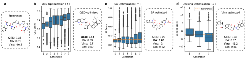
Figure 4: Examples of optimization runs. (a) Reference molecule. (b) QED optimization. (c) SA optimization. (d) Docking score optimization.

Binding MOAD

Results for the Binding MOAD dataset with experimentally determined binding complex data are reported in Table 1 as well. DiffSBDD generates highly diverse molecules but, unlike the CrossDocked case, docking scores are lower on average than corresponding reference ligands from this dataset. We believe the reason to be twofold: the Binding MOAD training set is much smaller and also contains more challenging ground-truth ligands (native binders) whereas CrossDocked complexes can have unrealistic protein-ligand interactions. This hypothesis is supported by the lower Vina scores of reference molecules from the synthetic dataset.

Generated molecules for two representative targets (PDB: 6c0b and PDB: 3gt9) are shown in Figure 3. The first target (PDB: 6c0b) is a human receptor which is involved in microbial infection (Chen et al., 2018) and possibly tumor suppression (Ding et al., 2016). The reference molecule, a long fatty acid (see Figure 3, bottom left panel) that aids receptor binding (Chen et al., 2018), has too high a number of rotatable bonds and low a number of hydrogen bond donors/acceptors to be considered a suitable drug (QED of 0.36). Our model however, generates drug-like (QED between 0.29-0.62) and suitably sized molecules by adding aromatic rings connected by a small number of rotatable bonds, which allows the molecules to adopt a complementary binding geometry and is entropically favourable (by reducing the degrees of freedom), a classic technique in medicinal chemistry (Ritchie & Macdonald, 2009).

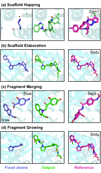
Figure 5: Examples of during molecular inpainting to accomplish (a) scaffold hopping, (b) scaffold elaboration, (c) fragment merging and (d) fragment growing. For each row, the left image shows the fixed atom input to the model, the middle image is the output (w$/$ inpainted region) and the right is an example from the PDB.

4.3 Molecule Optimization

We use our model to optimize exciting candidate molecules, a common task in drug discovery called lead optimization. This is when we take a compound found to have high binding affinity and optimize it for better ‘drug-like’ properties. We first noise the atom features and coordinates for $t$ steps (where $t$ is small) using the forward diffusion process. From this partially noised sample, we can then denoise the appropriate number of steps with the reverse process until $t=0$. This allows us to sample new candidates of various properties whilst staying in the same region of active chemical space, assuming $t$ is small (Appendix Figure 12). This approach is inspired by (Luo et al., 2022) but note this does not allow for direct optimization of specific properties. Instead, it can be regarded as an exploration around the local chemical space whilst maintaining high shape and chemical complementary via the conditional DDPM.

We extend this idea by combining the partial noising/denoising procedure with a simple evolutionary algorithm that optimizes for specific molecular properties. We find that our model performs well at this task out-of-the-box without requiring additional fine-tuning. As a showcase, we optimize a molecule in the test set targeting PDB 5ndu, a cancer therapeutic (Barone et al., 2020), which has low SA and QED scores, 0.31 and 0.35 respectively, but high binding affinity. Over a number of rounds of optimization, we can observe significant increases in QED (from 0.35 to mean of 0.43) whilst still maintaining high similarity to the original molecule (Figure 4a). We can also rescue the low synthetic accessibility score of the seed molecule by producing a battery of highly accessible molecules when selecting for SA. Finally, we observe that we can perform significant optimization of binding affinity after only a few rounds of optimization. Figures 4b-d show three optimization runs alongside representative molecules with substantially optimized scores (QED, SA or Vina) whilst maintaining comparable binding affinity and globally similar structures. Full details are provided in Appendix G.8.

4.4 Flexible molecule design with inpainting

In drug discovery it is very common to design molecules around previously identified potent substructures. For example, we may wish to design a scaffold around a set of functional groups (scaffold hopping) or extend an existing fragment to make a whole molecule (fragment growing). We can realise a number of these sub-tasks through molecular inpainting (see Section 3.3), whereby we can inpaint in and around fixed regions of the molecule to design whole molecules. Unlike previous methods, using DiffSBDD in this a way does not require retraining a new model on any specialized, usually synthetic, datasets. Rather, the simple definition of an arbitrary binary mask allows the method to generalize to any inpainting task whilst using a conditional DDPM trained on all protein-drug data. Four case studies are presented in Figure 5 as a proof-of-concept, with full methodological descriptions in Appendix C.2.

5 Conclusion

In this work, we propose DiffSBDD, an $SE(3)$-equivariant 3D-conditional diffusion model for structure-based drug design. We demonstrate the effectiveness of DiffSBDD in generating novel and diverse ligands with predicted high-affinity for given protein pockets on two datasets. We also show that a joint model in combination with an inpainting-based sampling approach can achieve competitive results to direct conditioning on a wide range of molecular metrics. Finally, we provide case studies that showcase the model’s versatility and applicability to downstream drug design tasks. Future work will attempt to study the performance in these domains further. We hope that this flexible approach to using DiffSBDD allows medicinal chemists to augment their domain expertise with a powerful data-driven diffusion model.

Appendix for
“Structure-based Drug Design with
Equivariant Diffusion Models”

Appendix A Variational Lower Bound

To maximise the likelihood of our training data, we aim at optimising the variational lower bound (VLB) (Kingma et al., 2021; Hoogeboom et al., 2022)

$$-\log p(\bm{z}_{\text{data}})\leq\underbrace{D_{\text{KL}}\big{(}q(\bm{z}_{T}|\bm{z}_{\text{data}})||p(\bm{z}_{T})\big{)}}_{\text{prior loss $\mathcal{L}_{\text{prior}}$}}\underbrace{-\mathbb{E}_{q(\bm{z}_{0}|\bm{z}_{\text{data}})}\big{[}\log p(\bm{z}_{\text{data}}|\bm{z}_{0})\big{]}}_{\text{reconstruction loss $\mathcal{L}_{0}$}}+\underbrace{\sum_{t=1}^{T}\mathcal{L}_{t}}_{\text{diffusion loss}}$$ (10)

with

$$\mathcal{L}_{t} =D_{\text{KL}}\big{(}q(\bm{z}_{t-1}|\bm{z}_{\text{data}},\bm{z}_{t})||p_{\theta}(\bm{z}_{t-1}|\hat{\bm{z}}_{\text{data}},\bm{z}_{t})\big{)}$$ (11)

$$=\mathbb{E}_{\bm{\epsilon}\sim\mathcal{N}(\bm{0},\bm{I})}\Big{[}\frac{1}{2}\Big{(}\frac{\text{SNR}(t-1)}{\text{SNR}(t)}-1\Big{)}||\bm{\epsilon}-\hat{\bm{\epsilon}}_{\theta}||^{2}\Big{]}$$ (12)

during training. The prior loss should always be close to zero and can be computed exactly in closed form while the reconstruction loss must be estimated as described in Hoogeboom et al. (2022). In practice, however, we simply minimise the mean squared error $\mathcal{L}_{\text{train}}=\frac{1}{2}||\bm{\epsilon}-\hat{\bm{\epsilon}}||^{2}$ while randomly sampling time steps $t\sim\mathcal{U}(0,\dots,T)$, which is equivalent up to a multiplicative factor.

Appendix B Note on Equivariance of the Conditional Model

The 3D-conditional model can achieve equivariance without the usual “subspace-trick”. The coordinates of pocket nodes provide a reference frame for all samples that can be used to translate them to a unique location (e.g. such that the pocket is centered at the origin: $\sum_{i}\bm{x}^{(P)}_{i}=\bm{0}$). By doing this for all training data, translation equivariance becomes irrelevant and the CoM-free subspace approach obsolete. To evaluate the likelihood of translated samples at inference time, we can first subtract the pocket’s center of mass from the whole system and compute the likelihood after this mapping. Similarly, for sampling molecules we can first generate a ligand in a CoM-free version of the pocket and move the whole system back to the original location of the pocket nodes to restore translation equivariance. As long as the mean of our Gaussian noise distribution $p(\bm{z}_{t}|\bm{z}^{(P)}_{\text{data}})=\mathcal{N}(\bm{\mu}(\bm{z}^{(P)}_{\text{data}}),\sigma^{2}\bm{I})$ depends equivariantly on the pocket node coordinates $\bm{x}^{(P)}$, $O(3)$-equivariance is satisfied as well (Appendix E). Since this change did not seem to affect the performance of the conditional model in our experiments, we decided to keep sampling in the linear subspace to ensure that the implementation is as similar as possible to the joint model, for which the subspace approach is necessary.

Appendix C Implementation Details

Molecule size

As part of a sample’s overall likelihood, we compute the empirical joint distribution of ligand and pocket nodes $p(N_{L},N_{P})$ observed in the training set and smooth it with a Gaussian filter ($\sigma=1$). In the conditional generation scenario, we derive the distribution $p(N_{L}|N_{P})$ and use it for likelihood computations.

For sampling, we can either fix molecule sizes manually or sample the number of ligand nodes from the same distribution given the number of nodes in the target pocket:

$$N_{L}\sim p(N_{L}|N_{P}).$$ (13)

For the experiments discussed in the main text, we increase the mean size of sampled molecules by 5 (CrossDocked) and 10 (Binding MOAD) atoms, respectively, to approximately match the sizes of molecules found in the test set. This modification makes the reported QuickVina scores more comparable as the in silico docking score is highly correlated with the molecular size, which is demonstrated in Figure 6. Average molecule sizes after applying the correction are shown in Table 2 together with corresponding values for generated molecules from other methods.

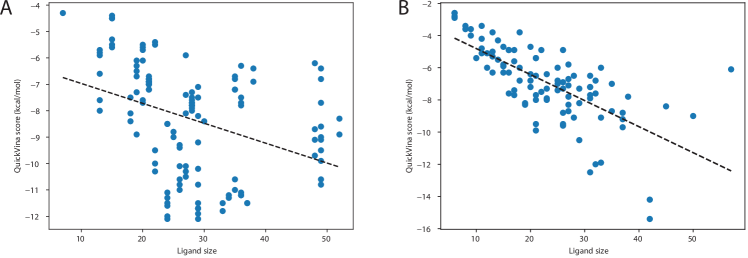
Figure 6: Correlation between ligand size and QuickVina score for reference molecules from the Binding MOAD (A) and CrossDocked (B) test sets.

Table 2: Average number of heavy atoms of generated molecules.

Method	CrossDocked	Binding MOAD
Test set	$22.75\pm 9.9$	$28.04\pm 10.2$
3D-SBDD (Luo et al., 2021)	$15.55\pm 6.1$	—
Pocket2Mol (Peng et al., 2022)	$18.09\pm 9.1$	—
GraphBP (Liu et al., 2022)	$18.62\pm 9.2$	$15.46\pm 6.2$
TargetDiff (Guan et al., 2023)	$24.15\pm 9.1$	—
DiffSBDD-cond ($C_{\alpha}$)	$24.69\pm 8.4$	$25.27\pm 7.8$
DiffSBDD-inpaint ($C_{\alpha}$)	$26.64\pm 8.8$	$26.80\pm 8.2$
DiffSBDD-cond	$24.40\pm 8.7$	$24.47\pm 7.9$
DiffSBDD-inpaint	$24.03\pm 9.1$	$25.14\pm 7.9$

Preprocessing

All molecules are expressed as graphs. For the $C_{\alpha}$ only model the node features for the protein are set as the one hot encoding of the amino acid type. The full atom model uses the same one hot encoding of atom types for ligand and protein nodes. We refrain from adding a categorical feature for distinguishing between protein and ligand atoms in this case and continue using two separate MLPs for embedding the node features instead.

Noise schedule

We use the pre-defined polynomial noise schedule introduced in (Hoogeboom et al., 2022):

$$\tilde{\alpha}_{t}=1-\Big{(}\frac{t}{T}\Big{)}^{2},\quad t=0,...,T$$ (14)

Following (Nichol & Dhariwal, 2021; Hoogeboom et al., 2022), values of $\tilde{\alpha}_{t|s}^{2}=\big{(}\frac{\tilde{\alpha}_{t}}{\tilde{\alpha}_{s}}\big{)}^{2}$ are clipped between 0.001 and 1 for numerical stability near $t=T$, and $\tilde{\alpha}_{t}$ is recomputed as

$$\tilde{\alpha}_{t}=\prod_{\tau=0}^{t}\tilde{\alpha}_{\tau|\tau-1}.$$ (15)

A tiny offset $\epsilon=10^{-5}$ is used to avoid numerical problems at $t=0$ defining the final noise schedule:

$$\alpha_{t}^{2}=(1-2\epsilon)\cdot\tilde{\alpha}_{t}^{2}+\epsilon.$$ (16)

Feature scaling

We scale the node type features $\bm{h}$ by a factor of 0.25 relative to the coordinates $\bm{x}$ which was empirically found to improve model performance in previous work (Hoogeboom et al., 2022). To train joint probability models in the all-atom scenario, it was necessary to scale down the coordinates (and corresponding distance cutoffs) by a factor of 0.2 instead in order to avoid introducing too many edges in the graph near the end of the diffusion process at $t=T$.

Hyperparameters

Hyperparameters for all presented models are summarized in Table 3. Training takes about $2.5\text{\,}\mathrm{h}$/$3.8\text{\,}\mathrm{h}$ (cond/inpaint) per 100 epochs on a single NVIDIA V100 for Binding MOAD in the $C_{\alpha}$ scenario and $11.5\text{\,}\mathrm{h}$/$14.7\text{\,}\mathrm{h}$ per 100 epochs with full atom pocket representation on two V100 GPUs. For CrossDocked, 100 training epochs take approximately $6\text{\,}\mathrm{h}$/$8\text{\,}\mathrm{h}$ in the $C_{\alpha}$ case and $48\text{\,}\mathrm{h}$/$60\text{\,}\mathrm{h}$ per 100 epochs on a single NVIDIA A100 GPU with all atom pocket representation.

Table 3: DiffSBDD hyperparameters.

CrossDocked Binding MOAD Cond Inpaint Cond ($C_{\alpha}$) Inpaint ($C_{\alpha}$) Cond Inpaint Cond ($C_{\alpha}$) Inpaint ($C_{\alpha}$) No. layers 5 5 6 6 6 6 5 5 Joint embedding dim. 32 32 128 128 128 128 32 32 Hidden dim. 128 128 256 256 192 192 128 128 Learning rate $10^{-3}$ $10^{-3}$ $10^{-3}$ $10^{-3}$ $5\cdot 10^{-4}$ $5\cdot 10^{-4}$ $5\cdot 10^{-4}$ $5\cdot 10^{-4}$ Weight decay $10^{-12}$ $10^{-12}$ $10^{-12}$ $10^{-12}$ $10^{-12}$ $10^{-12}$ $10^{-12}$ $10^{-12}$ Diffusion steps 500 500 500 500 500 500 500 500 Edges (ligand-ligand) fully connected fully connected fully connected fully connected fully connected fully connected fully connected fully connected Edges (ligand-pocket) $<$5\text{\,}\mathrm{\text{Å}}$$ $<$5\text{\,}\mathrm{\text{Å}}$$ $<$5\text{\,}\mathrm{\text{Å}}$$ $<$5\text{\,}\mathrm{\text{Å}}$$ $<$7\text{\,}\mathrm{\text{Å}}$$ $<$7\text{\,}\mathrm{\text{Å}}$$ $<$8\text{\,}\mathrm{\text{Å}}$$ $<$8\text{\,}\mathrm{\text{Å}}$$ Edges (pocket-pocket) $<$5\text{\,}\mathrm{\text{Å}}$$ $<$5\text{\,}\mathrm{\text{Å}}$$ $<$5\text{\,}\mathrm{\text{Å}}$$ $<$5\text{\,}\mathrm{\text{Å}}$$ $<$4\text{\,}\mathrm{\text{Å}}$$ $<$4\text{\,}\mathrm{\text{Å}}$$ $<$8\text{\,}\mathrm{\text{Å}}$$ $<$8\text{\,}\mathrm{\text{Å}}$$ Epochs 1000 1000 1000 1000 1000 1000 1000 1000

Postprocessing

For postprocessing of generated molecules, we use a similar procedure as in (Luo et al., 2021). Given a list of atom types and coordinates, bonds are first added using OpenBabel (O’Boyle et al., 2011). We then use RDKit to sanitise molecules and filter for the largest molecular fragment.

C.1 Resampling

Here, we briefly recapitulate the resampling algorithm introduced in Ref. (Lugmayr et al., 2022). The key intuition is that inpainting with the replacement method combines a generated part with an independently sampled latent representation of the known part. Even though the neural network tries to reconcile these two components in every step of the denoising trajectory, it cannot succeed because the same issue reoccurs in the following step. Lugmayr et al. (2022) thus propose to apply the neural network several times before proceeding to the next noise level, allowing the DDPM to preserve more conditional information and move the sample closer to the data distribution again. The procedure is summarized in Algorithm 1 including our center of mass adjustment discussed in Section 3.3.

Algorithm 1 Sampling with the replacement method and resampling iterations. $r$ denotes the number of resampling steps and $\mathcal{M}$ is a set of indices of all atoms we want to fix. Note that samples from the generative process $p_{\theta}(\bm{z}_{t-1}|\bm{z}_{t})$ are assumed to be CoM-free.

$r$, $\mathcal{M}$

$\bm{z}_{T}\sim\mathcal{N}(\bm{0},\bm{I})$

for $t=T,...,1$ do

     for $k=1,...,r$ do

         $\bm{z}_{t-1}^{\text{fixed}}\sim q(\bm{z}_{t-1}|\bm{z}_{\text{data}})$ $\triangleright$ Sample known context

         $\bm{z}_{t-1}^{\text{gen}}\sim p_{\theta}(\bm{z}_{t-1}|\bm{z}_{t})$ $\triangleright$ Sample generated part

         $\tilde{\bm{x}}_{t-1}^{\text{fixed}}=\bm{x}_{t-1}^{\text{fixed}}+\frac{1}{n}\sum_{i\in\mathcal{M}}\bm{x}_{t-1,i}^{\text{gen}}-\frac{1}{n}\sum_{i\in\mathcal{M}}\bm{x}_{t-1,i}^{\text{fixed}}$ $\triangleright$ Adjust center of mass

         $\bm{z}_{t-1}=[\tilde{\bm{z}}_{t-1}^{\text{fixed}},\bm{z}_{t-1,i\notin\mathcal{M}}^{\text{gen}}]$ $\triangleright$ Combine

         if $k<r$ then

              $\bm{z}_{t}\sim q(\bm{z}_{t}|\bm{z}_{t-1})$ $\triangleright$ Apply noise and repeat

         end if

     end for

end for

return $\bm{z}_{0}$

Number of resampling steps

To empirically study the effect of the number of resampling iterations applied, we generated ligands for all test pockets with $r=1$, $r=5$, and $r=10$ resampling steps, respectively. Because the resampling strategy slows down sampling approximately by a factor of $r$, we used the striding technique proposed by Nichol & Dhariwal (2021) and reduced the number of denoising steps proportionally to $r$. Nichol & Dhariwal (2021) showed that this approach reduces the number of sampling steps significantly without sacrificing sample quality. In our case, it allows us to retain sampling speed while increasing the number of resampling steps.

To gauge the effect of resampling for molecule generation we show the distribution of RMSD values between the center of mass of reference molecules and generated molecules in Figure 7. The unmodified replacement method ($r=1$) produces molecules that are clearly farther away from the presumed pocket center than the conditional model. Increasing $r$ moves the mean distance closer to the average displacement of molecules from the conditional method. This effect seems to saturate at $r=10$ which is in line with the results obtained for images (Lugmayr et al., 2022).

Table 4 shows that neither the additional resampling steps nor the shortened denoising trajectory degrade the performance on the reported molecular metrics. The average docking scores even improve slightly which might reflect better positioning of generated ligands in the pockets prior to docking. The same model trained with $T=500$ diffusion steps was used in all three cases.

Table 4: Evaluation of generated molecules for target pockets from the CrossDocked (C.D.) and Binding MOAD (B.M.) test sets with the inpainting approach and $C_{\alpha}$ pocket representation for varying numbers of resampling steps $r$ and denoising steps $T$. For Binding MOAD, these experiments have been conducted without the adjustment of molecule sizes described in Section C, which explains the lower average Vina scores compared to Table 1.

$r$ $T$ Vina Score (kcal/mol, $\downarrow$) QED ($\uparrow$) SA ($\uparrow$) Lipinski ($\uparrow$) Diversity ($\uparrow$) Time (s, $\downarrow$) C.D. 1 500 $-5.830\pm 2.47$ $0.403\pm 0.18$ $0.552\pm 0.13$ $4.620\pm 0.81$ $0.808\pm 0.06$ $97.434\pm 39.79$ 5 100 $-6.872\pm 2.43$ $0.444\pm 0.19$ $0.551\pm 0.12$ $4.654\pm 0.72$ $0.766\pm 0.06$ $96.205\pm 39.22$ 10 50 $-7.177\pm 3.28$ $0.556\pm 0.20$ $0.729\pm 0.12$ $4.742\pm 0.59$ $0.718\pm 0.07$ $94.481\pm 38.86$ B.M. 1 500 $-5.810\pm 2.00$ $0.468\pm 0.16$ $0.627\pm 0.14$ $4.839\pm 0.49$ $0.851\pm 0.04$ $40.298\pm 13.52$ 5 100 $-6.082\pm 2.01$ $0.537\pm 0.16$ $0.701\pm 0.13$ $4.924\pm 0.31$ $0.855\pm 0.05$ $45.074\pm 21.14$ 10 50 $-6.192\pm 2.24$ $0.560\pm 0.16$ $0.737\pm 0.13$ $4.941\pm 0.27$ $0.859\pm 0.05$ $41.490\pm 14.32$

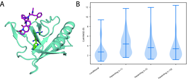
Figure 7: (A) Example of a generated molecule (green) without additional resampling steps and the reference molecule (magenta) from the target PDB 5ncf. The generated molecule is not placed in the target pocket but in the protein core. (B) RMSD between reference molecules’ center of mass and generated molecules’ center of mass for the conditional model and inpaining model with varying numbers of resampling steps $r$. The pocket representation is $C_{\alpha}$ in all cases.

C.2 Flexible molecule design with inpainting

Scaffold hopping

Molecular scaffolds, also called Bemis-Murcko scaffolds, are often a defined as the molecular core of a compound to which R (functional) groups are attached via attachment points (Bemis & Murcko, 1996). Defining the scaffold allows us to study the key functional groups mediating receptor binding and uncover structure-activity relationships (SAR). Once understood, we can fix the molecular decorations and build new scaffolds to support those functional groups in place, thus allowing us to find structurally distinct compounds that have the same/similar activity. Such a task is known as scaffold hopping and is a central process in medicinal chemistry which allows us to discover structurally novel compounds (Böhm et al., 2004).

In our case study (Figure 5a) we perform scaffold hopping around the functional groups of PDB:2gm1. Such a task could be simplified by partially noising then denoising the existing high performing scaffold and may even be desirable if there are medicinal or synthetic chemistry constraints in place. However, to demonstrate the power of our approach, we instead choose to sample a brand new scaffold de novo by sampling $n$ (where $n$ is the number of atoms present in the original scaffold) new atoms from $\mathcal{N}(\bm{0},\bm{I})$ whilst fixing the functional groups during inpainting.

Scaffold elaboration

Scaffold elaboration can be seen as the inverse problem of scaffold hopping. Here, we have a known scaffold of ideal structure and we wish to enumerate/optimize the functional groups at or around the attachment points to improve activity (Abel & Bhat, 2017).

For our case study (Figure 5b), we perform optimisation of all the R-groups attached to the molecule in PDB:5ndu. $n$ new atoms are sampled de novo as above while the scaffold is kept fixed. Note, the attachment points can be moved if deemed suitable by our learnt model.

Fragment merging

Fragment merging is the task of combining fragments with an overlapping binding site (Li, 2020).

For the fragment merging example, instead of masking existing molecules, we instead take fragments from an experimental fragment screen against the non structural protein 3 (NSP3) from SARS-CoV-2 (Schuller et al., 2021). Using two fragments as input (PDB:5rue and PDB:5rsw) we successfully replicate the fragment merge undertaking in Gahbauer et al. (2023) which was accomplished using the chemoinformatics-based approach Fragmenstein.

Fragment growing

Fragment growing is the task of adding chemical groups/whole other fragments to a seed fragment to improve properties (Li, 2020).

For our case study (Figure 5d), we perform fragment growing in two directions around the central fragment in PDB:5ndu. The molecule is broken into three fragments using the Breaking Retrosynthetically Interesting Chemical Substructures (BRICS) (Degen et al., 2008) protocol. Out of these, the middle fragment is fixed whilst the two outer fragment, plus accompanying linkers, are redesigned. Here, we elect to showcase the second regime of partially noising/denoising the inpainted region, allowing us to partially redesign the two peripheral fragments whilst fixing the central one, which could be useful for a number of retrosynthetic and activity reasons.

Appendix D Binding MOAD Dataset

We curate a dataset of experimentally determined complexed protein-ligand structures from Binding MOAD (Hu et al., 2005). We keep pockets with valid and moderately ‘drug-like’ ligands with QED score $>0.3$. We further discard small molecules that contain atom types $\notin\{C,N,O,S,B,Br,Cl,P,I,F\}$ as well as binding pockets with non-standard amino acids. We define binding pockets as the set of residues that have any atom within $8\text{\,}\mathrm{\text{Å}}$ of any ligand atom. Ligand redundancy is reduced by randomly sampling at most 50 molecules with the same chemical component identifier (3-letter-code). After removing corrupted entries that could not be processed, $40\,344$ training pairs and 130 testing pairs remain. A validation set of size 246 is used to monitor estimated log-likelihoods during training. The split is made to ensure different sets do not contain proteins from the same Enzyme Commission Number (EC Number) main class.

Appendix E Proofs

In the following proofs we do not consider categorical node features $\bm{h}$ as only the positions $\bm{x}$ are subject to equivariance constraints. Furthermore, we do not distinguish between the zeroth latent representation $\bm{x}_{0}$ and data domain representations $\bm{x}_{\text{data}}$ for ease of notation, and simply drop the subscripts.

E.1 $O(3)$-equivariance of the prior probability

The isotropic Gaussian prior $p(\bm{x}^{(L)}_{T}|\bm{x}^{(P)})=\mathcal{N}(\bm{\mu}(\bm{x^{(P)}}),\sigma^{2}\bm{I})$ is equivariant to rotations and reflections represented by an orthogonal matrix $\bm{R}\in\mathbb{R}^{3\times 3}$ as long as $\bm{\mu}(\bm{R}\bm{x}^{(P)})=\bm{R}\bm{\mu}(\bm{x}^{(P)})$ because:

$$p(\bm{R}\bm{x}^{(L)}_{T}|\bm{R}\bm{x}^{(P)}) =\frac{1}{\sqrt{(2\pi)^{N_{L}}\sigma^{2}}}\exp\Big{(}-\frac{1}{2\sigma^{2}}||\bm{R}\bm{x}^{(L)}_{T}-\bm{\mu}(\bm{R}\bm{x}^{(P)})||^{2}\Big{)}$$

$$=\frac{1}{\sqrt{(2\pi)^{N_{L}}\sigma^{2}}}\exp\Big{(}-\frac{1}{2\sigma^{2}}||\bm{R}\bm{x}^{(L)}_{T}-\bm{R}\bm{\mu}(\bm{x}^{(P)})||^{2}\Big{)}$$

$$=\frac{1}{\sqrt{(2\pi)^{N_{L}}\sigma^{2}}}\exp\Big{(}-\frac{1}{2\sigma^{2}}||\bm{R}\big{(}\bm{x}^{(L)}_{T}-\bm{\mu}(\bm{x}^{(P)})\big{)}||^{2}\Big{)}$$

$$=\frac{1}{\sqrt{(2\pi)^{N_{L}}\sigma^{2}}}\exp\Big{(}-\frac{1}{2\sigma^{2}}||\bm{x}^{(L)}_{T}-\bm{\mu}(\bm{x}^{(P)})||^{2}\Big{)}$$

$$=p(\bm{x}^{(L)}_{T}|\bm{x}^{(P)}).$$

Here we used $||\bm{R}\bm{x}||_{2}=||\bm{x}||_{2}$ for orthogonal $\bm{R}$.

E.2 $O(3)$-equivariance of the transition probabilities

The denoising transition probabilities from time step $t$ to $s<t$ are defined as isotropic normal distributions:

$$p_{\theta}(\bm{x}^{(L)}_{t-1}|\bm{x}^{(L)}_{t},\hat{\bm{x}}^{(L)},\bm{x}^{(P)})=\mathcal{N}(\bm{x}^{(L)}_{t-1}|\bm{\mu}_{t\rightarrow s}(\bm{x}^{(L)}_{t},\hat{\bm{x}}^{(L)},\bm{x}^{(P)}),\sigma_{t\rightarrow s}^{2}\bm{I}).$$ (17)

Therefore, $p_{\theta}(\bm{x}^{(L)}_{t-1}|\bm{x}^{(L)}_{t},\hat{\bm{x}}^{(L)},\bm{x}^{(P)})$ is $O(3)$-equivariant by a similar argument to Section E.1 if $\bm{\mu}_{t\rightarrow s}$ is computed equivariantly from the three-dimensional context.

Recalling the definition of $\bm{\mu}_{t\rightarrow s}=\frac{\alpha_{t|s}\sigma_{s}^{2}}{\sigma_{t}^{2}}\bm{x}^{(L)}_{t}+\frac{\alpha_{s}\sigma_{t|s}^{2}}{\sigma_{t}^{2}}\hat{\bm{x}}^{(L)}$, we can prove its equivariance as follows:

$$\bm{\mu}_{t\rightarrow s}(\bm{R}\bm{x}^{(L)}_{t},\bm{R}\bm{x}^{(P)}) =\frac{\alpha_{t|s}\sigma_{s}^{2}}{\sigma_{t}^{2}}\bm{R}\bm{x}^{(L)}_{t}+\frac{\alpha_{s}\sigma_{t|s}^{2}}{\sigma_{t}^{2}}\hat{\bm{x}}^{(L)}(\bm{R}\bm{x}_{t}^{(L)},\bm{R}\bm{x}^{(P)})$$

$$=\frac{\alpha_{t|s}\sigma_{s}^{2}}{\sigma_{t}^{2}}\bm{R}\bm{x}^{(L)}_{t}+\frac{\alpha_{s}\sigma_{t|s}^{2}}{\sigma_{t}^{2}}\bm{R}\hat{\bm{x}}^{(L)}(\bm{x}_{t}^{(L)},\bm{x}^{(P)})\quad\text{(equivariance of $\hat{\bm{x}}^{(L)}$)}$$

$$=\bm{R}\Big{(}\frac{\alpha_{t|s}\sigma_{s}^{2}}{\sigma_{t}^{2}}\bm{x}^{(L)}_{t}+\frac{\alpha_{s}\sigma_{t|s}^{2}}{\sigma_{t}^{2}}\hat{\bm{x}}^{(L)}(\bm{x}_{t}^{(L)},\bm{x}^{(P)})\Big{)}$$

$$=\bm{R}\bm{\mu}_{t\rightarrow s}(\bm{x}^{(L)}_{t},\bm{x}^{(P)}),$$

where $\hat{\bm{x}}^{(L)}$ defined as $\hat{\bm{x}}^{(L)}=\frac{1}{\alpha_{t}}\bm{x}_{t}^{(L)}-\frac{\sigma_{t}}{\alpha_{t}}\hat{\bm{\epsilon}}$ is equivariant because:

$$\hat{\bm{x}}^{(L)}(\bm{R}\bm{x}_{t}^{(L)},\bm{R}\bm{x}^{(P)}) =\frac{1}{\alpha_{t}}\bm{R}\bm{x}_{t}^{(L)}-\frac{\sigma_{t}}{\alpha_{t}}\hat{\bm{\epsilon}}(\bm{R}\bm{x}_{t}^{(L)},\bm{R}\bm{x}^{(P)},t)$$

$$=\frac{1}{\alpha_{t}}\bm{R}\bm{x}_{t}^{(L)}-\frac{\sigma_{t}}{\alpha_{t}}\bm{R}\hat{\bm{\epsilon}}(\bm{x}_{t}^{(L)},\bm{x}^{(P)},t)\quad\text{($\hat{\bm{\epsilon}}$ predicted by equivariant neural network)}$$

$$=\bm{R}\Big{(}\frac{1}{\alpha_{t}}\bm{x}_{t}^{(L)}-\frac{\sigma_{t}}{\alpha_{t}}\hat{\bm{\epsilon}}(\bm{x}_{t}^{(L)},\bm{x}^{(P)},t)\Big{)}$$

$$=\bm{R}\hat{\bm{x}}^{(L)}(\bm{x}_{t}^{(L)},\bm{x}^{(P)}).$$

E.3 $O(3)$-equivariance of the learned likelihood

Let $\bm{R}\in\mathbb{R}^{3\times 3}$ be an orthogonal matrix representing an element $g$ from the general orthogonal group $O(3)$. We obtain the marginal probability density of the Markovian denoising process as follows

$$p_{\theta}(\bm{x}^{(L)}_{0}|\bm{x}^{(P)}) =\int p(\bm{x}^{(L)}_{T}|\bm{x}^{(P)})p_{\theta}(\bm{x}^{(L)}_{0:T-1}|\bm{x}^{(L)}_{T},\bm{x}^{(P)})\text{d}\bm{x}_{1:T}$$

$$=\int p(\bm{x}^{(L)}_{T}|\bm{x}^{(P)})\prod_{t=1}^{T}p_{\theta}(\bm{x}^{(L)}_{t-1}|\bm{x}^{(L)}_{t},\bm{x}^{(P)})\text{d}\bm{x}_{1:T}$$

and the sample’s likelihood is $O(3)$-equivariant:

$$p_{\theta}(\bm{R}\bm{x}^{(L)}_{0}|\bm{R}\bm{x}^{(P)}) =\int p(\bm{R}\bm{x}^{(L)}_{T}|\bm{R}\bm{x}^{(P)})\prod_{t=1}^{T}p_{\theta}(\bm{R}\bm{x}^{(L)}_{t-1}|\bm{R}\bm{x}^{(L)}_{t},\bm{R}\bm{x}^{(P)})\text{d}\bm{x}_{1:T}$$

$$=\int p(\bm{x}^{(L)}_{T}|\bm{x}^{(P)})\prod_{t=1}^{T}p_{\theta}(\bm{R}\bm{x}^{(L)}_{t-1}|\bm{R}\bm{x}^{(L)}_{t},\bm{R}\bm{x}^{(P)})\text{d}\bm{x}_{1:T}\quad\text{(equivariant prior)}$$

$$=\int p(\bm{x}^{(L)}_{T}|\bm{x}^{(P)})\prod_{t=1}^{T}p_{\theta}(\bm{x}^{(L)}_{t-1}|\bm{x}^{(L)}_{t},\bm{x}^{(P)})\text{d}\bm{x}_{1:T}\quad\text{(equivariant transition probabilities)}$$

$$=p_{\theta}(\bm{x}^{(L)}_{0}|\bm{x}^{(P)})$$

Appendix F $SE(3)$-equivariant Graph Neural Network

Chiral molecules cannot be superimposed by any combination of rotations and translations. Instead they are mirrored along a stereocenter, axis, or plane. As chirality can significantly alter a molecule’s chemical properties, we use a variant of the $E(3)$-equivariant graph neural networks (Satorras et al., 2021) presented in Equations (3)-(5) that is sensitive to reflections and hence $SE(3)$-equivariant. We change the coordinate update equation, Equ. (5), of standard EGNNs in the following way

$$\bm{x}_{i}^{l+1}=\bm{x}_{i}^{l}+\sum_{j\neq i}\frac{\bm{x}_{i}^{l}-\bm{x}_{j}^{l}}{d_{ij}+1}\phi_{x}^{d}(\bm{h}^{l}_{i},\bm{h}^{l}_{j},d_{ij}^{2},a_{ij})+\frac{(\bm{x}_{i}^{l}-\bar{\bm{x}}^{l})\times(\bm{x}_{j}^{l}-\bar{\bm{x}}^{l})}{||(\bm{x}_{i}^{l}-\bar{\bm{x}}^{l})\times(\bm{x}_{j}^{l}-\bar{\bm{x}}^{l})||+1}\phi_{x}^{\times}(\bm{h}^{l}_{i},\bm{h}^{l}_{j},d_{ij}^{2},a_{ij}),$$ (18)

where $\bar{\bm{x}}^{l}$ denotes the center of mass of all nodes at layer $l$. This modification makes the EGNN layer sensitive to reflections while staying close to the original formalism. Since the resulting graph neural networks are only equivariant to the $SE(3)$ group, we will hereafter call them SE(3)GNNs for short.

F.1 Discussion of Equivariance

Here we study how the suggested change in the coordinate update equation breaks reflection symmetry while preserving equivariance to rotations. Messages and scalar feature updates (Equations (3) and (4)) remain $E(3)$-invariant as in the original model and are therefore not considered in this section. We analyze transformations composed of a translation by $\bm{t}\in\mathbb{R}^{3}$ and a rotation/reflection by an orthogonal matrix $\bm{R}\in\mathbb{R}^{3\times 3}$ with $\bm{R}^{T}\bm{R}=\bm{I}$. The output at layer $l+1$ given the transformed input $\bm{R}\bm{x}^{l}_{i}+\bm{t}$ at layer $l$ is calculated as:

$$\bm{R}\bm{x}^{l}_{i}+\bm{t}+\sum_{j\neq i}\frac{\bm{R}\bm{x}^{l}_{i}+\bm{t}-(\bm{R}\bm{x}^{l}_{j}+\bm{t})}{d_{ij}+1}\phi_{x}^{d}(\cdot)+\frac{(\bm{R}\bm{x}^{l}_{i}+\bm{t}-(\bm{R}\bar{\bm{x}}^{l}+\bm{t}))\times(\bm{R}\bm{x}^{l}_{j}+\bm{t}-(\bm{R}\bar{\bm{x}}^{l}+\bm{t}))}{Z^{\times}_{ij}+1}\phi_{x}^{\times}(\cdot)$$ (19)

$$=\bm{R}\bm{x}^{l}_{i}+\bm{t}+\sum_{j\neq i}\frac{\bm{R}(\bm{x}^{l}_{i}-\bm{x}^{l}_{j})}{d_{ij}+1}\phi_{x}^{d}(\cdot)+\frac{(\bm{R}\bm{x}^{l}_{i}-\bm{R}\bar{\bm{x}}^{l})\times(\bm{R}\bm{x}^{l}_{j}-\bm{R}\bar{\bm{x}}^{l})}{Z^{\times}_{ij}+1}\phi_{x}^{\times}(\cdot)$$ (20)

$$=\bm{R}\bm{x}^{l}_{i}+\bm{t}+\sum_{j\neq i}\frac{\bm{R}(\bm{x}^{l}_{i}-\bm{x}^{l}_{j})}{d_{ij}+1}\phi_{x}^{d}(\cdot)+\frac{\det(\bm{R})\bm{R}\big{(}(\bm{x}^{l}_{i}-\bar{\bm{x}}^{l})\times(\bm{x}^{l}_{j}-\bar{\bm{x}}^{l})\big{)}}{Z^{\times}_{ij}+1}\phi_{x}^{\times}(\cdot)$$ (21)

$$=\bm{R}\bm{x}_{i}^{l+1}+\bm{t}+\big{(}\det(\bm{R})-1\big{)}\sum_{j\neq i}\frac{\bm{R}\big{(}(\bm{x}^{l}_{i}-\bar{\bm{x}}^{l})\times(\bm{x}^{l}_{j}-\bar{\bm{x}}^{l})\big{)}}{Z^{\times}_{ij}+1}.$$ (22)

This result shows that the output coordinates are only equivariantly transformed if $\bm{R}$ is orientation preserving, i.e. $\det(\bm{R})=1$. If $\bm{R}$ is a reflection ($\det(\bm{R})=-1$), coordinates will be updated with an additional summand that breaks the symmetry.

The learnable coefficients $\phi_{x}^{d}(\bm{h}^{l}_{i},\bm{h}^{l}_{j},d_{ij}^{2},a_{ij})$ and $\phi_{x}^{\times}(\bm{h}^{l}_{i},\bm{h}^{l}_{j},d_{ij}^{2},a_{ij})$ only depend on relative distances and are therefore $E(3)$-invariant. Their arguments are represented with the “$\cdot$” symbol for brevity. Likewise, the normalization factor $||(\bm{x}_{i}^{l}-\bar{\bm{x}}^{l})\times(\bm{x}_{j}^{l}-\bar{\bm{x}}^{l})||$ is abbreviated as $Z^{\times}_{ij}$. Already in the first line we used the fact that the mean transforms equivariantly. Furthermore, we use $\bm{R}\bm{a}\times\bm{R}\bm{b}=\det(\bm{R})\bm{R}(\bm{a}\times\bm{b})$ in the second step, which can be derived as follows:

$$\bm{x}^{T}(\bm{R}\bm{a}\times\bm{R}\bm{b}) =\det(\underbrace{[\bm{x},\bm{R}\bm{a},\bm{R}\bm{b}]}_{\in\mathbb{R}^{3\times 3}})$$ (23)

$$=\det(\bm{R}[\bm{R}^{T}\bm{x},\bm{a},\bm{b}])$$ (24)

$$=\det(\bm{R})\det([\bm{R}^{T}\bm{x},\bm{a},\bm{b}])$$ (25)

$$=\det(\bm{R})\Big{(}\bm{x}^{T}\bm{R}(\bm{a}\times\bm{b})\Big{)}$$ (26)

$$=\bm{x}^{T}\Big{(}\det(\bm{R})\bm{R}(\bm{a}\times\bm{b})\Big{)}$$ (27)

The stated property of the cross product follows because this derivation is true for all $\bm{x}\in\mathbb{R}^{3}$.

Table 5: Accuracy on the R/S classification task. Results in the first section are taken from (Adams et al., 2021) and included for reference.

Model	R/S Accuracy (%)
ChIRo	$98.5$
SchNet	$54.4$
DimeNet++	$65.7$
SphereNet	$98.2$
EGNN	$50.4$
SE(3)GNN	$83.4$

F.2 Empirical Results

To show the effectiveness of this architecture on a simple toy example, we repeat the classification experiment by Adams et al. (2021) who train neural networks to classify tetrahedral chiral centers as right-handed (rectus, ‘R’) or left-handed (sinister, ‘S’). We closely follow their data split and experimental set-up and only replace the classifier with EGNN and SE(3)GNNs, respectively. The results in Table 5 clearly demonstrate that the $SE(3)$-equivariant EGNN is capable of solving this task (without any hyperparameter optimization) whereas the $E(3)$-equivariant version does not do better than random guessing.

Appendix G Extended results

G.1 Additional Experimental Details

The numbers of available molecules differ slightly between different methods due to computational issues or missing molecules in the available baseline sets. More precisely, on average $100$, $99.7$, $100$ and $100$ molecules have been evaluated per pocket for DiffSBDD-cond, Diff-SBDD-inpaint, DiffSBDD-cond ($C_{\alpha}$), and DiffSBDD-inpaint ($C_{\alpha}$), respectively. For Pocket2Mol, $98.4$ molecules are available per pocket. The set of 3D-SBDD molecules does not contain generated ligands for two test pockets. For the remaining $98$ pockets, $89.9$ molecules are available on average. For GraphBP, $86.1$ molecules are evaluated per pocket. For Binding MOAD, $100$ molecules were available per pocket for evaluation of all DiffSBDD models except for the conditional model with full atomic pocket representation ($99.9$ on average). We could further evaluate $88$ molecules from GraphBP per pocket.

G.2 Additional Molecular Metrics

In addition to the molecular properties discussed in Section 4 we assess the models’ ability to produce novel and valid molecules using four simple metrics: validity, connectivity, uniqueness, and novelty. Validity measures the proportion of generated molecules that pass basic tests by RDKit–mostly ensuring correct valencies. Connectivity is the proportion of valid molecules that do not contain any disconnected fragments. We convert every valid and connected molecule from a graph into a canonical SMILES string representation, count the number unique occurrences in the set of generated molecules and compare those to the training set SMILES to compute uniqueness and novelty respectively.

Table 6 shows that only a small fraction of all generated molecules is invalid and must be discarded for downstream processing. A much larger percentage of molecules is fragmented but, since we can simply select and process the largest fragments in these cases, low connectivity does not necessarily affect the efficiency of the generative process. Moreover, all models produce diverse sets of molecules unseen in the training set.

Table 6: Basic molecular metrics for generated small molecules given a $C_{\alpha}$ and full atom representation of the protein pocket.

Model	Validity	Connectivity	Uniqueness	Novelty
CrossDocked test set	100%	100%	96%	96.88%
DiffSBDD-cond ($C_{\alpha}$)	95.52%	79.52%	99.99%	99.97%
DiffSBDD-inpaint ($C_{\alpha}$)	99.18%	98.25%	99.52%	99.97%
DiffSBDD-cond	97.10%	78.27%	99.98%	99.99%
DiffSBDD-inpaint	92.99%	67.52%	100%	100%
Binding MOAD test set	97.69%	100%	38.58%	77.55%
DiffSBDD-cond ($C_{\alpha}$)	94.41%	77.38%	100%	100%
DiffSBDD-inpaint ($C_{\alpha}$)	98.36%	91.60%	99.99%	99.98%
DiffSBDD-cond	96.32%	63.37%	100%	100%
DiffSBDD-inpaint	93.88%	75.60%	100%	100%

G.3 Octanol-water partition coefficient

The octanol-water partition coefficient ($\log P$) is a measure of lipophilicity and is commonly reported for potential drug candidates (Wildman & Crippen, 1999). We summarize this property for our generated molecules in Table 7.

Table 7: LogP values of generated molecules.

	CrossDocked	Binding MOAD
Test set	$0.894\pm 2.73$	$1.785\pm 2.62$
3D-SBDD (Luo et al., 2021)	$0.273\pm 2.01$	—
Pocket2Mol (Peng et al., 2022)	$1.720\pm 1.97$	—
GraphBP (Liu et al., 2022)	$0.664\pm 1.12$	$0.347\pm 0.77$
TargetDiff (Guan et al., 2023)	$1.371\pm 2.34$	—
DiffSBDD-cond ($C_{\alpha}$)	$1.232\pm 2.22$	$1.596\pm 2.15$
DiffSBDD-inpaint ($C_{\alpha}$)	$3.494\pm 2.16$	$2.791\pm 2.42$
DiffSBDD-cond	$1.209\pm 2.04$	$1.150\pm 2.28$
DiffSBDD-inpaint	$2.498\pm 2.64$	$3.084\pm 2.18$

G.4 Vina scores for subsets of generated molecules

Table 8 summarizes Vina docking scores for different subsets of molecules with the highest scores among all molecules generated for a given pocket. While there is a significant number of poorly scoring molecules among all generated candidates, these results show that DiffSBDD also produces a large population with high predicted binding affinity. Furthermore, the performance gap between DiffSBDD and competing methods increases as the selection becomes stricter.

Table 8: Docking score evaluation for different subsets of generated molecules for targets from the CrossDocked and Binding MOAD test sets. ^∗ denotes that we re-evaluate the generated ligands provided by the authors.

top-1 top-5 top-10 top-20 top-50 top-100 CrossDocked Test set $-6.871\pm 2.32$ — — — — — 3D-SBDD (Luo et al., 2021)^∗ $-7.797\pm 2.53$ $-7.491\pm 2.42$ $-7.289\pm 2.34$ $-7.003\pm 2.23$ $-6.527\pm 2.02$ $-5.888\pm 1.91$ Pocket2Mol (Peng et al., 2022)^∗ $-9.225\pm 3.4$ $-8.92\pm 3.27$ $-8.712\pm 3.18$ $-8.446\pm 3.09$ $-7.937\pm 2.93$ $-7.058\pm 2.8$ GraphBP (Liu et al., 2022) $-8.989\pm 1.77$ $-7.746\pm 1.53$ $-7.165\pm 1.4$ $-6.575\pm 1.29$ $-5.691\pm 1.23$ $-4.719\pm 4.03$ TargetDiff (Guan et al., 2023)^∗ $-10.980\pm 2.86$ $-10.134\pm 2.62$ $-9.669\pm 2.55$ $-9.135\pm 2.46$ $-8.252\pm 2.37$ $-7.318\pm 2.47$ DiffSBDD-cond ($C_{\alpha}$) $-9.633\pm 1.87$ $-9.106\pm 1.79$ $-8.796\pm 1.75$ $-8.415\pm 1.70$ $-7.752\pm 1.69$ $-6.770\pm 2.73$ DiffSBDD-inpaint ($C_{\alpha}$) $-10.048\pm 1.90$ $-9.527\pm 1.84$ $-9.233\pm 1.82$ $-8.875\pm 1.81$ $-8.240\pm 1.85$ $-7.177\pm 3.28$ DiffSBDD-cond $-10.249\pm 2.48$ $-9.5180\pm 2.26$ $-9.120\pm 2.16$ $-8.666\pm 2.07$ $-7.922\pm 1.96$ $-6.950\pm 2.06$ DiffSBDD-inpaint gray!30 $-11.176\pm 2.82$ gray!30 $-10.394\pm 2.67$ gray!30 $-9.927\pm 2.59$ gray!30 $-9.393\pm 2.52$ gray!30 $-8.510\pm 2.43$ gray!30 $-7.333\pm 2.56$ Binding MOAD Test set $-8.412\pm 2.03$ — — — — — GraphBP (Liu et al., 2022) $-7.802\pm 1.16$ $-7.001\pm 1.00$ $-6.629\pm 0.95$ $-6.213\pm 0.91$ $-5.553\pm 0.90$ $-4.843\pm 2.24$ DiffSBDD-cond ($C_{\alpha}$) $-9.375\pm 1.42$ $-8.888\pm 1.36$ $-8.587\pm 1.34$ $-8.237\pm 1.31$ $-7.643\pm 1.29$ $-6.863\pm 1.59$ DiffSBDD-inpaint ($C_{\alpha}$) $-10.059\pm 1.28$ $-9.475\pm 1.33$ $-9.124\pm 1.35$ $-8.699\pm 1.37$ $-8.018\pm 1.41$ $-6.926\pm 3.39$ DiffSBDD-cond $-10.276\pm 2.53$ $-9.582\pm 2.35$ $-9.184\pm 2.23$ $-8.724\pm 2.11$ $-7.983\pm 1.96$ $-7.171\pm 1.89$ DiffSBDD-inpaint gray!30 $-11.177\pm 2.44$ gray!30 $-10.302\pm 2.24$ gray!30 $-9.840\pm 2.18$ gray!30 $-9.331\pm 2.11$ gray!30 $-8.550\pm 2.01$ gray!30 $-7.309\pm 4.03$

G.5 Agreement of generated and docked conformations

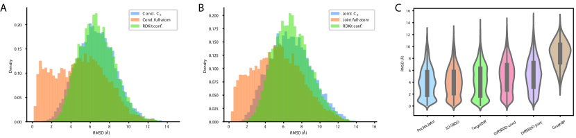
Figure 8: RMSD between generated and docked conformations for the CrossDocked dataset. Full-atom models are compared to $C_{\alpha}$ models as well as a baseline of random RDKit conformers of the molecules generated by the $C_{\alpha}$-model. (A) Conditionally trained models. (B) Joint probability models with inpainting. (C) Comparison between DiffSBDD given full atomic context and other models for de novo design.

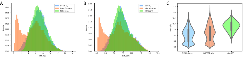
Figure 9: RMSD between generated and docked conformations for the Binding MOAD dataset. Full-atom models are compared to $C_{\alpha}$ models as well as a baseline of random RDKit conformers of the molecules generated by the $C_{\alpha}$-model. (A) Conditionally trained models. (B) Joint probability models with inpainting. (C) Comparison between DiffSBDD given full atomic context and GraphBP.

Here we discuss an alternative way of using QuickVina for assessing the quality of the conditional generation procedure besides its in silico docking score. We compare the generated raw conformations to the best scoring QuickVina docking pose and plot the distribution of resulting RMSD values in Figures 8 and 9. As a baseline, the procedure is repeated for RDKit conformers of the same molecules with identical center of mass. For a large percentage of molecules generated by the all-atom models, QuickVina agrees with the predicted bound conformations, leaving them almost unchanged (RMSD below $2\text{\,}\mathrm{\text{Å}}$). This demonstrates successful conditioning on the geometry of the given protein pockets. For the $C_{\alpha}$-only models results are less convincing. They produce poses that only slightly improve upon conformers lacking pocket-context. Likely, this is caused by atomic clashes with the proteins’ side chains that QuickVina needs to resolve. Figure 8C shows that DiffSBDD performs competitively on this metric, albeit with slightly higher mean RMSDs than some of the methods we compare to.

G.6 Random generated molecules

Randomly selected molecules generated with our method and 2 baseline methods (3D-SBDD and Pocket2Mol) when trained with CrossDocked are presented in Figure 10.

Figure 10: Generated molecules for ten randomly chosen targets in the CrossDocked test set. For each target, three randomly selected generated molecules from three models are shown.

G.7 Distribution of docking scores by target

We present extensive evaluation of the docking scores for our generated molecules in Figure 11. We evaluate all models trained with a given dataset first against all targets (Figure 11A+C) and 8 randomly chosen targets (Figure 11B+D). We note that the all-atom model trained using CrossDocked data outperforms all other methods. Unsurprisingly, model performance is highly target dependent, likely varying with properties like pocket geometry, size, charge, and hydrophbicity, which would affect the propensity of generating high affinity molecules.

Figure 11: Docking scores of generated molecules for various methods trained on the CrossDocked (A-B) and Binding MOAD (C-D) datasets. (A) Violin plot of docking scores for all four methods trained using CrossDocked. (B) Same as before but for eight randomly chosen targets sorted by mean score. (C) Violin plot of docking scores for all four methods trained using Binding MOAD. (D) Same as before but for eight randomly chosen targets sorted by mean score.

G.8 Optimization

We demonstrate the effect the number of noising/denoising steps ($t$) has on various molecular properties in Figure 12. We test all values of $t$ at intervals of 10 steps and 200 molecules are sampled at every timestep. Note this does not allow for explicit optimization of any particular property unless combined with the evolutionary algorithm.

During the evolutionary algorithm, at the end of every generation the top 10 docking molecules are used to seed the next population. Every seed molecule is elaborated into 20 new candidates with a randomly chosen $t$ between 10 and 150. To make the first population, we start with the single reference molecule and sample 200 new molecules with $t$ chosen as above.

Figure 12: Effect of number of noising/denoising steps on molecule properties.

Appendix H Related Work

Diffusion Models for Molecules

Inspired by non-equilibrium thermodynamics, diffusion models have been proposed to learn data distributions by modeling a denoising (reverse diffusion) process and have achieved remarkable success in a variety of tasks such as image, audio synthesis and point cloud generation (Kingma et al., 2021; Kong et al., 2021; Luo & Hu, 2021). Recently, efforts have been made to utilize diffusion models for molecule design (Du et al., 2022b). Specifically, Hoogeboom et al. (2022) propose a diffusion model with an equivariant network that operates both on continuous atomic coordinates and categorical atom types to generate new molecules in 3D space. Torsional Diffusion (Jing et al., 2022) focuses on a conditional setting where molecular conformations (atomic coordinates) are generated from molecular graphs (atom types and bonds). Similarly, 3D diffusion models have been applied to generative design of larger biomolecular structures, such as antibodies (Luo et al., 2022) and other proteins (Anand & Achim, 2022; Trippe et al., 2022).

Structure-based Drug Design

Structure-based Drug Design (SBDD) (Ferreira et al., 2015; Anderson, 2003) relies on the knowledge of the 3D structure of the biological target obtained either through experimental methods or high-confidence predictions using homology modelling (Kelley et al., 2015). Candidate molecules are then designed to bind with high affinity and specificity to the target using interactive software (Kalyaanamoorthy & Chen, 2011) and often human-based intuition (Ferreira et al., 2015). Recent advances in deep generative models have brought a new wave of research that model the conditional distribution of ligands given biological targets and thus enable de novo structure-based drug design. Most of recent work consider this task as a sequential generation problem and design a variety of generative methods including autoregressive models, reinforcement learning, etc., to generate ligands inside protein pockets atom by atom (Drotár et al., 2021; Luo et al., 2021; Li et al., 2021; Peng et al., 2022).

Geometric Deep Learning for Drug Discovery

Geometric deep learning refers to incorporating geometric priors in neural architecture design that respects symmetry and invariance, thus reduces sample complexity and eliminates the need for data augmentation (Bronstein et al., 2021). It has been prevailing in a variety of drug discovery tasks from virtual screening to de novo drug design as symmetry widely exists in the representation of drugs. One line of work introduces graph and geometry priors and designs message passing neural networks and equivariant neural networks that are permutation- and translation-, rotation-, reflection-equivariant, respectively (Duvenaud et al., 2015; Gilmer et al., 2017; Satorras et al., 2021; Lapchevskyi et al., 2020; Du et al., 2022a). These architectures have been widely used in representing biomolecules from small molecules to proteins (Atz et al., 2021) and solving downstream tasks such as molecular property prediction (Schütt et al., 2018; Klicpera et al., 2020), binding pose prediction (Stärk et al., 2022) or molecular dynamics (Batzner et al., 2022; Holdijk et al., 2022). Another line of work focuses on generative design of new molecules (Du et al., 2022b, c). More specifically, molecule design is formulated as a graph or geometry generation problem, following either a one-shot generation strategy that generates graphs (atom and bond features) in one step or attempting to generate them sequentially.

References

- Abel & Bhat (2017) Abel, R. and Bhat, S. Free energy calculation guided virtual screening of synthetically feasible ligand r-group and scaffold modifications: an emerging paradigm for lead optimization. In Annual Reports in Medicinal Chemistry, volume 50, pp. 237–262. Elsevier, 2017.
- Adams et al. (2021) Adams, K., Pattanaik, L., and Coley, C. W. Learning 3d representations of molecular chirality with invariance to bond rotations. arXiv preprint arXiv:2110.04383, 2021.
- Alhossary et al. (2015) Alhossary, A., Handoko, S. D., Mu, Y., and Kwoh, C.-K. Fast, accurate, and reliable molecular docking with quickvina 2. Bioinformatics, 31(13):2214–2216, 2015.
- Anand & Achim (2022) Anand, N. and Achim, T. Protein structure and sequence generation with equivariant denoising diffusion probabilistic models. arXiv preprint arXiv:2205.15019, 2022.
- Anderson (2003) Anderson, A. C. The process of structure-based drug design. Chemistry & biology, 10(9):787–797, 2003.
- Atz et al. (2021) Atz, K., Grisoni, F., and Schneider, G. Geometric deep learning on molecular representations. Nature Machine Intelligence, 3(12):1023–1032, 2021.
- Barone et al. (2020) Barone, M., Müller, M., Chiha, S., Ren, J., Albat, D., Soicke, A., Dohmen, S., Klein, M., Bruns, J., van Dinther, M., et al. Designed nanomolar small-molecule inhibitors of ena/vasp evh1 interaction impair invasion and extravasation of breast cancer cells. Proceedings of the National Academy of Sciences, 117(47):29684–29690, 2020.
- Batzner et al. (2022) Batzner, S., Musaelian, A., Sun, L., Geiger, M., Mailoa, J. P., Kornbluth, M., Molinari, N., Smidt, T. E., and Kozinsky, B. E (3)-equivariant graph neural networks for data-efficient and accurate interatomic potentials. Nature communications, 13(1):1–11, 2022.
- Bemis & Murcko (1996) Bemis, G. W. and Murcko, M. A. The properties of known drugs. 1. molecular frameworks. Journal of medicinal chemistry, 39(15):2887–2893, 1996.
- Böhm et al. (2004) Böhm, H.-J., Flohr, A., and Stahl, M. Scaffold hopping. Drug discovery today: Technologies, 1(3):217–224, 2004.
- Bronstein et al. (2021) Bronstein, M. M., Bruna, J., Cohen, T., and Veličković, P. Geometric deep learning: Grids, groups, graphs, geodesics, and gauges. arXiv preprint arXiv:2104.13478, 2021.
- Chen et al. (2018) Chen, P., Tao, L., Wang, T., Zhang, J., He, A., Lam, K.-h., Liu, Z., He, X., Perry, K., Dong, M., et al. Structural basis for recognition of frizzled proteins by clostridium difficile toxin b. Science, 360(6389):664–669, 2018.
- Corso et al. (2022) Corso, G., Stärk, H., Jing, B., Barzilay, R., and Jaakkola, T. Diffdock: Diffusion steps, twists, and turns for molecular docking. arXiv preprint arXiv:2210.01776, 2022.
- Degen et al. (2008) Degen, J., Wegscheid-Gerlach, C., Zaliani, A., and Rarey, M. On the art of compiling and using’drug-like’chemical fragment spaces. ChemMedChem: Chemistry Enabling Drug Discovery, 3(10):1503–1507, 2008.
- Ding et al. (2016) Ding, L.-C., Huang, X.-Y., Zheng, F.-F., Xie, J., She, L., Feng, Y., Su, B.-H., Zheng, D.-L., and Lu, Y.-G. Fzd2 inhibits the cell growth and migration of salivary adenoid cystic carcinomas. Oncology Reports, 35(2):1006–1012, 2016.
- Drotár et al. (2021) Drotár, P., Jamasb, A. R., Day, B., Cangea, C., and Liò, P. Structure-aware generation of drug-like molecules. arXiv preprint arXiv:2111.04107, 2021.
- Du et al. (2022a) Du, W., Zhang, H., Du, Y., Meng, Q., Chen, W., Zheng, N., Shao, B., and Liu, T.-Y. Se (3) equivariant graph neural networks with complete local frames. In International Conference on Machine Learning, pp. 5583–5608. PMLR, 2022a.
- Du et al. (2022b) Du, Y., Fu, T., Sun, J., and Liu, S. Molgensurvey: A systematic survey in machine learning models for molecule design. arXiv preprint arXiv:2203.14500, 2022b.
- Du et al. (2022c) Du, Y., Liu, X., Shah, N., Liu, S., Zhang, J., and Zhou, B. Chemspace: Interpretable and interactive chemical space exploration. 2022c.
- Duvenaud et al. (2015) Duvenaud, D. K., Maclaurin, D., Iparraguirre, J., Bombarell, R., Hirzel, T., Aspuru-Guzik, A., and Adams, R. P. Convolutional networks on graphs for learning molecular fingerprints. Advances in neural information processing systems, 28, 2015.
- Ferreira et al. (2015) Ferreira, L. G., Dos Santos, R. N., Oliva, G., and Andricopulo, A. D. Molecular docking and structure-based drug design strategies. Molecules, 20(7):13384–13421, 2015.
- Francoeur et al. (2020) Francoeur, P. G., Masuda, T., Sunseri, J., Jia, A., Iovanisci, R. B., Snyder, I., and Koes, D. R. Three-dimensional convolutional neural networks and a cross-docked data set for structure-based drug design. Journal of Chemical Information and Modeling, 60(9):4200–4215, 2020.
- Gahbauer et al. (2023) Gahbauer, S., Correy, G. J., Schuller, M., Ferla, M. P., Doruk, Y. U., Rachman, M., Wu, T., Diolaiti, M., Wang, S., Neitz, R. J., et al. Iterative computational design and crystallographic screening identifies potent inhibitors targeting the nsp3 macrodomain of sars-cov-2. Proceedings of the National Academy of Sciences, 120(2):e2212931120, 2023.
- Gaudelet et al. (2021) Gaudelet, T., Day, B., Jamasb, A. R., Soman, J., Regep, C., Liu, G., Hayter, J. B. R., Vickers, R., Roberts, C., Tang, J., Roblin, D., Blundell, T. L., Bronstein, M. M., and Taylor-King, J. P. Utilizing graph machine learning within drug discovery and development. Briefings in Bioinformatics, 22(6), May 2021. doi: 10.1093/bib/bbab159. URL https://doi.org/10.1093/bib/bbab159.
- Gilmer et al. (2017) Gilmer, J., Schoenholz, S. S., Riley, P. F., Vinyals, O., and Dahl, G. E. Neural message passing for quantum chemistry. In International conference on machine learning, pp. 1263–1272. PMLR, 2017.
- Guan et al. (2023) Guan, J., Qian, W. W., Peng, X., Su, Y., Peng, J., and Ma, J. 3d equivariant diffusion for target-aware molecule generation and affinity prediction. arXiv preprint arXiv:2303.03543, 2023.
- Ho et al. (2020) Ho, J., Jain, A., and Abbeel, P. Denoising diffusion probabilistic models. Advances in Neural Information Processing Systems, 33:6840–6851, 2020.
- Holdijk et al. (2022) Holdijk, L., Du, Y., Hooft, F., Jaini, P., Ensing, B., and Welling, M. Path integral stochastic optimal control for sampling transition paths. arXiv preprint arXiv:2207.02149, 2022.
- Hoogeboom et al. (2022) Hoogeboom, E., Satorras, V. G., Vignac, C., and Welling, M. Equivariant diffusion for molecule generation in 3d. In International Conference on Machine Learning, pp. 8867–8887. PMLR, 2022.
- Hu et al. (2005) Hu, L., Benson, M. L., Smith, R. D., Lerner, M. G., and Carlson, H. A. Binding moad (mother of all databases). Proteins: Structure, Function, and Bioinformatics, 60(3):333–340, 2005.
- Igashov et al. (2022) Igashov, I., Stärk, H., Vignac, C., Satorras, V. G., Frossard, P., Welling, M., Bronstein, M., and Correia, B. Equivariant 3d-conditional diffusion models for molecular linker design. arXiv preprint arXiv:2210.05274, 2022.
- Irwin & Shoichet (2005) Irwin, J. J. and Shoichet, B. K. Zinc- a free database of commercially available compounds for virtual screening. Journal of chemical information and modeling, 45(1):177–182, 2005.
- Jing et al. (2022) Jing, B., Corso, G., Chang, J., Barzilay, R., and Jaakkola, T. Torsional diffusion for molecular conformer generation. arXiv preprint arXiv:2206.01729, 2022.
- Kalyaanamoorthy & Chen (2011) Kalyaanamoorthy, S. and Chen, Y.-P. P. Structure-based drug design to augment hit discovery. Drug discovery today, 16(17-18):831–839, 2011.
- Kelley et al. (2015) Kelley, L. A., Mezulis, S., Yates, C. M., Wass, M. N., and Sternberg, M. J. The phyre2 web portal for protein modeling, prediction and analysis. Nature protocols, 10(6):845–858, 2015.
- Kingma et al. (2021) Kingma, D., Salimans, T., Poole, B., and Ho, J. Variational diffusion models. Advances in neural information processing systems, 34:21696–21707, 2021.
- Klicpera et al. (2020) Klicpera, J., Groß, J., and Günnemann, S. Directional message passing for molecular graphs. arXiv preprint arXiv:2003.03123, 2020.
- Köhler et al. (2020) Köhler, J., Klein, L., and Noé, F. Equivariant flows: exact likelihood generative learning for symmetric densities. In International conference on machine learning, pp. 5361–5370. PMLR, 2020.
- Kong et al. (2021) Kong, Z., Ping, W., Huang, J., Zhao, K., and Catanzaro, B. Diffwave: A versatile diffusion model for audio synthesis. In International Conference on Learning Representations, 2021.
- Landrum et al. (2016) Landrum, G. et al. Rdkit: Open-source cheminformatics software. 2016.
- Lapchevskyi et al. (2020) Lapchevskyi, K., Miller, B., Geiger, M., and Smidt, T. Euclidean neural networks (e3nn) v1. 0. Technical report, Lawrence Berkeley National Lab.(LBNL), Berkeley, CA (United States), 2020.
- Li (2020) Li, Q. Application of fragment-based drug discovery to versatile targets. Frontiers in molecular biosciences, 7:180, 2020.
- Li et al. (2021) Li, Y., Pei, J., and Lai, L. Structure-based de novo drug design using 3d deep generative models. Chemical science, 12(41):13664–13675, 2021.
- Lipinski et al. (2012) Lipinski, C. A., Lombardo, F., Dominy, B. W., and Feeney, P. J. Experimental and computational approaches to estimate solubility and permeability in drug discovery and development settings. Advanced drug delivery reviews, 64:4–17, 2012.
- Liu et al. (2022) Liu, M., Luo, Y., Uchino, K., Maruhashi, K., and Ji, S. Generating 3d molecules for target protein binding. arXiv preprint arXiv:2204.09410, 2022.
- Lu et al. (2022) Lu, W., Wu, Q., Zhang, J., Rao, J., Li, C., and Zheng, S. Tankbind: Trigonometry-aware neural networks for drug-protein binding structure prediction. bioRxiv, 2022.
- Lugmayr et al. (2022) Lugmayr, A., Danelljan, M., Romero, A., Yu, F., Timofte, R., and Van Gool, L. Repaint: Inpainting using denoising diffusion probabilistic models. In Proceedings of the IEEE/CVF Conference on Computer Vision and Pattern Recognition, pp. 11461–11471, 2022.
- Luo & Hu (2021) Luo, S. and Hu, W. Diffusion probabilistic models for 3d point cloud generation. In Proceedings of the IEEE/CVF Conference on Computer Vision and Pattern Recognition, pp. 2837–2845, 2021.
- Luo et al. (2021) Luo, S., Guan, J., Ma, J., and Peng, J. A 3d generative model for structure-based drug design. Advances in Neural Information Processing Systems, 34:6229–6239, 2021.
- Luo et al. (2022) Luo, S., Su, Y., Peng, X., Wang, S., Peng, J., and Ma, J. Antigen-specific antibody design and optimization with diffusion-based generative models. bioRxiv, 2022.
- Lyne (2002) Lyne, P. D. Structure-based virtual screening: an overview. Drug discovery today, 7(20):1047–1055, 2002.
- Nichol & Dhariwal (2021) Nichol, A. Q. and Dhariwal, P. Improved denoising diffusion probabilistic models. In International Conference on Machine Learning, pp. 8162–8171. PMLR, 2021.
- O’Boyle et al. (2011) O’Boyle, N. M., Banck, M., James, C. A., Morley, C., Vandermeersch, T., and Hutchison, G. R. Open babel: An open chemical toolbox. Journal of cheminformatics, 3(1):1–14, 2011.
- Peng et al. (2022) Peng, X., Luo, S., Guan, J., Xie, Q., Peng, J., and Ma, J. Pocket2mol: Efficient molecular sampling based on 3d protein pockets. arXiv preprint arXiv:2205.07249, 2022.
- Ragoza et al. (2022) Ragoza, M., Masuda, T., and Koes, D. R. Generating 3d molecules conditional on receptor binding sites with deep generative models. Chemical science, 13(9):2701–2713, 2022.
- Ritchie & Macdonald (2009) Ritchie, T. J. and Macdonald, S. J. The impact of aromatic ring count on compound developability–are too many aromatic rings a liability in drug design? Drug discovery today, 14(21-22):1011–1020, 2009.
- Satorras et al. (2021) Satorras, V. G., Hoogeboom, E., and Welling, M. E (n) equivariant graph neural networks. In International conference on machine learning, pp. 9323–9332. PMLR, 2021.
- Schuller et al. (2021) Schuller, M., Correy, G. J., Gahbauer, S., Fearon, D., Wu, T., Díaz, R. E., Young, I. D., Carvalho Martins, L., Smith, D. H., Schulze-Gahmen, U., et al. Fragment binding to the nsp3 macrodomain of sars-cov-2 identified through crystallographic screening and computational docking. Science advances, 7(16):eabf8711, 2021.
- Schütt et al. (2018) Schütt, K. T., Sauceda, H. E., Kindermans, P.-J., Tkatchenko, A., and Müller, K.-R. Schnet–a deep learning architecture for molecules and materials. The Journal of Chemical Physics, 148(24):241722, 2018.
- Serre et al. (1977) Serre, J.-P. et al. Linear representations of finite groups, volume 42. Springer, 1977.
- Shoichet (2004) Shoichet, B. K. Virtual screening of chemical libraries. Nature, 432(7019):862–865, 2004.
- Sohl-Dickstein et al. (2015) Sohl-Dickstein, J., Weiss, E., Maheswaranathan, N., and Ganguli, S. Deep unsupervised learning using nonequilibrium thermodynamics. In International Conference on Machine Learning, pp. 2256–2265. PMLR, 2015.
- Song et al. (2020) Song, Y., Sohl-Dickstein, J., Kingma, D. P., Kumar, A., Ermon, S., and Poole, B. Score-based generative modeling through stochastic differential equations. arXiv preprint arXiv:2011.13456, 2020.
- Stärk et al. (2022) Stärk, H., Ganea, O., Pattanaik, L., Barzilay, R., and Jaakkola, T. Equibind: Geometric deep learning for drug binding structure prediction. In International Conference on Machine Learning, pp. 20503–20521. PMLR, 2022.
- Steinegger & Söding (2017) Steinegger, M. and Söding, J. MMseqs2 enables sensitive protein sequence searching for the analysis of massive data sets. Nature Biotechnology, 35(11):1026–1028, October 2017. doi: 10.1038/nbt.3988. URL https://doi.org/10.1038/nbt.3988.
- Trippe et al. (2022) Trippe, B. L., Yim, J., Tischer, D., Broderick, T., Baker, D., Barzilay, R., and Jaakkola, T. Diffusion probabilistic modeling of protein backbones in 3d for the motif-scaffolding problem. arXiv preprint arXiv:2206.04119, 2022.
- Wang et al. (2022) Wang, J., Lisanza, S., Juergens, D., Tischer, D., Watson, J. L., Castro, K. M., Ragotte, R., Saragovi, A., Milles, L. F., Baek, M., et al. Scaffolding protein functional sites using deep learning. Science, 377(6604):387–394, 2022.
- Wildman & Crippen (1999) Wildman, S. A. and Crippen, G. M. Prediction of physicochemical parameters by atomic contributions. Journal of chemical information and computer sciences, 39(5):868–873, 1999.
- Xu et al. (2022) Xu, M., Yu, L., Song, Y., Shi, C., Ermon, S., and Tang, J. Geodiff: A geometric diffusion model for molecular conformation generation. arXiv preprint arXiv:2203.02923, 2022.