Noise Injection as a Probe of Deep Learning Dynamics

Abstract

We propose a new method to probe the learning mechanism of Deep Neural Networks (DNN) by perturbing the system using Noise Injection Nodes (NINs). These nodes inject uncorrelated noise via additional optimizable weights to existing feed-forward network architectures, without changing the optimization algorithm. We find that the system displays distinct phases during training, dictated by the scale of injected noise. We first derive expressions for the dynamics of the network and utilize a simple linear model as a test case. We find that in some cases, the evolution of the noise nodes is similar to that of the unperturbed loss, thus indicating the possibility of using NINs to learn more about the full system in the future.

1 Introduction

Deep learning has proven exceedingly successful, leading to dramatic improvements in multiple domains. Nevertheless, our current theoretical understanding of deep learning methods has remained unsatisfactory. Specifically, the training of DNNs is a highly opaque procedure, with few metrics, beyond curvature evolution [1, 2, 3, 4, 5, 6, 7], available to describe how a network evolves as it trains.

An interesting attempt at parameterizing the interplay between training dynamics and generalization was explored in the seminal work of Ref. [8], which demonstrated that when input data was corrupted by adding random noise, the generalization error deteriorated in correlation with its strength. Noise injection has gained further traction in recent years, both as a means of effective regularization  [9, 10, 11, 12, 13, 14, 15, 16, 17, 18], as well as a route towards understanding DNN dynamics and generalization. For instance, label noise has been shown to affect the implicit bias of Stochastic Gradient Descent (SGD) [19, 20, 21, 22, 23], as sparse solutions appear to be preferred over those which reduce the Euclidean norm, in certain cases.

In this work, we take another step along this direction, by allowing the network to actively regulate the effects of the injected noise during training. Concretely, we define Noise Injection Nodes (NINs), whose output is a random variable, chosen sample-wise from a given distribution. These NINs are connected to existing feed-forward DNNs via trainable Noise Injection Weights (NIWs). The network is subsequently trained to perform a classification/regression task using vanilla SGD.

We study such systems both numerically and analytically, providing a detailed analytic understanding for a simple linear network. Our main results, partly summarized in Fig. 1, are as follows:

1. The system exhibits 4 NIN-related phases, depending mostly on the strength of the injected noise.

2. In two of the phases, the NIWs evolve to small values, implying that a well-trained network is able to recognize that the noise contains no useful information within it.

3. For those two phases, the NIW dynamics is dictated by the local curvature of the training loss function.

Item Item (ii) may be expected if the NIN is re-randomized at each training epoch, yet we find essentially the same behavior repeated even when the NIN values are generated only once and fixed before training, putting them on equal footing with actual data inputs, as shown in Fig. 1 (center,right). It appears that while the system might in principle be able to memorize the specific noise samples, optimization dynamics still prefer to suppress them. This implies a relation between the NIN reduction mechanism and the network’s ability to generalize, to be explored further in future works.

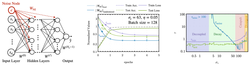
Figure 1: Schematic of a generic DNN, with the addition of a single NIN connected via NIWs. Center: Example evolution displaying a decay behavior for both the NIWs and the losses within the decay phase of the system discussed below and with a fixed noise strength, $\sigma_{\epsilon}$. Two cases are shown: re-initialized NIN at every epoch, and fixed value NIN. The similar behavior of the systems in both cases (blue and light blue points respectively) hint at a potent relation between the NIWs evolution and generalization. The blue, green and violet stars indicate the NIW, test loss and training loss decay time-scales. The three solid curves are fits to exponential decays, while the data is represented with points. Right: The different decay times as a function of the noise injection magnitude. The four shaded regions indicate the four phases of the system discussed in Sec. 3. The results are shown for a 3-hidden layer ReLU MLP with CE loss, trained on FMNIST to $100\text{\,}\mathrm{\char 37\relax}$ training accuracy.

2 Noise Injection Weights Evolution

Consider a DNN with parameters $\boldsymbol{\theta}=\{W^{(\ell)},b^{(\ell)}\in\mathbb{R}^{d_{\ell}\times d_{\ell+1}},\mathbb{R}^{d_{\ell+1}}|\ell=0,\dotsc,N_{L}-1\}$, corresponding to the weights and biases, and $N_{L}$ layers, defined by its single sample loss function $\mathcal{L}:\mathbb{R}^{d_{\mathrm{in}}}\to\mathbb{R}$ and optimized under SGD to perform a supervised learning task. Here, at each SGD iteration, a mini-batch $\mathcal{B}$ consists of a set of labeled examples, $\{(\boldsymbol{x}_{i},\boldsymbol{y}_{i})\}_{i=1}^{|\mathcal{B}|}\subseteq\mathbb{R}^{d_{\mathrm{in}}}\times\mathbb{R}^{d_{\mathrm{label}}}$.

We study the simple case of connecting a given NIN to a specific layer, denoted as $\ell_{\rm NI}$, via a NIW vector $W_{\mathrm{NI}}\in\mathbb{R}^{1\times d_{\ell_{\mathrm{NI}}+1}}$ (see Fig. 1, left). In this setup, the injected noise is taken as a random scalar variable, $\epsilon$, sampled repeatedly at each SGD training epoch from a chosen distribution. The NIWs’ evolution is best studied via their effect on preactivations, defined as $\boldsymbol{z}^{(\ell)}=W^{(\ell)}\cdot\boldsymbol{x}^{(\ell)}+b^{(\ell)}$. When a NIN is added, the preactivations at layer $\ell_{\mathrm{NI}}$ are subsequently shifted to $\boldsymbol{z}^{(\ell_{\rm{NI}})}\to\boldsymbol{z}^{(\ell_{\mathrm{NI}})}+W_{\rm{NI}}\epsilon$.

For a single NIN connected at layer $\ell_{\mathrm{NI}}$, the batch-averaged loss function can be written as a series expansion in the noise translation parameter

$$L({\boldsymbol{\theta}},{W_{\mathrm{NI}}}) =\frac{1}{|\mathcal{B}|}\sum_{\begin{subarray}{c}\{\boldsymbol{x},\epsilon,\boldsymbol{y}\}\in\mathcal{B}\end{subarray}}\mathcal{L}(\tilde{\boldsymbol{\theta}};\boldsymbol{z}^{(\ell_{\rm{NI}})}+{W_{\rm{NI}}}\epsilon,\boldsymbol{y})$$ (1)

$$=L({\boldsymbol{\theta}})+\frac{1}{|\mathcal{B}|}\sum_{\begin{subarray}{c}\{\boldsymbol{x},\epsilon,\boldsymbol{y}\}\in\mathcal{B}\end{subarray}}\sum_{k=1}^{\infty}\frac{(\epsilon{W^{T}_{\rm{NI}}}\cdot\nabla_{{\boldsymbol{z}^{(\ell_{\rm{NI}})}}})^{k}}{k!}\mathcal{L}(\boldsymbol{\theta};{\boldsymbol{x}},\epsilon,{\boldsymbol{y}}),$$

where ${\tilde{\boldsymbol{\theta}}}=\boldsymbol{\theta}\setminus\{W^{(\ell_{\rm{NI}})}\}$ and $L(\boldsymbol{\theta})$ is the loss function in the absence of a NIN. Focusing on a distribution with zero mean for the NIN (e.g., $\epsilon\sim\mathcal{N}(0,\sigma_{\epsilon}^{2})$) and performing the batch averaging on each term, we arrive at the update rule for the NIWs from the noisy loss expansion

$$W_{\rm{NI}}^{(t+1)}=W_{\rm{NI}}^{(t)}-\eta\frac{\sigma_{\epsilon}\Phi}{\sqrt{|\mathcal{B}|}}\sqrt{\langle(\boldsymbol{\textsl{g}}_{\ell_{\rm{NI}}}^{(t)})^{2}\rangle}-\frac{\eta\sigma^{2}_{\epsilon}}{2}\left\langle\mathcal{H}_{\ell_{\rm{NI}}}^{(t)}\right\rangle W_{\rm{NI}}^{(t)}+\dots.$$ (2)

Here, batch averaging is denoted by $\langle\,\dotsi\rangle$, $\Phi$ is a random variable with zero mean and unit variance, and $\sigma^{2}_{\epsilon}$ is the variance of the injected noise. We denote the network-dependent local gradient and Hessian at the NIN layer as

$${\boldsymbol{\textsl{g}}}_{\ell_{\rm{NI}}}=\nabla_{{\boldsymbol{z}}^{(\ell_{\rm{NI}})}}\mathcal{L}({\boldsymbol{\theta}};{\boldsymbol{x}},{\boldsymbol{y}}),\qquad{{\mathcal{H}_{\ell_{\rm{NI}}}}}={\nabla_{\boldsymbol{z}^{(\ell_{\rm{NI}})}}\nabla^{T}_{\boldsymbol{z}^{(\ell_{\rm{NI}})}}}\mathcal{L}(\boldsymbol{\theta};\boldsymbol{x},\boldsymbol{y}).$$ (3)

A more complete derivation, along with a proof for the $1/\sqrt{\mathcal{B}}$ scaling of odd terms in the expansion is given in App. C.

Terminating the expansion in Eq. 2 at 2nd order need not be valid for large $\sigma_{\epsilon}$. We thus proceed by studying a linear test case for which the 2nd order expansion is precise. The persistence of analogous network behavior, and in particular its phases, for a more realistic setup is confirmed empirically.

3 Linear Toy Model

Consider a two-layer DNN with linear activations and layer widths ($d_{0,1}=1$) and no biases ($b=0$), tasked with univariate linear regression, and with a single NIN connected to the first layer ($\ell_{\mathrm{NI}}=0$). The data consists of a set of training samples $\{(x_{i},y_{i})\in\mathbb{R}\times\mathbb{R}\}_{i=1}^{m}$, and we sample $x_{i}$ and the noise $\epsilon_{i}$ from the normal distributions, $x_{i},\epsilon_{i}\sim\mathcal{N}(0,\sigma_{x,\epsilon}^{2})$. The corresponding data labels are given by a linear transformation of the inputs $y_{i}=M\cdot x_{i}$ with a fixed $M\in\mathbb{R}$. This regression problem is solved by minimizing the empirical loss, taken as the Mean Squared Error (MSE),

$$L_{\mathrm{MSE}}=\frac{1}{2|\mathcal{B}|}\sum_{i\in\mathcal{B}}(w^{(1)}(w^{(0)}\cdot x_{i}+w_{\rm{NI}}\epsilon_{i})-y_{i})^{2},$$ (4)

with optimal solution $w^{(1)}_{*}w^{(0)}_{*}=M,w_{\mathrm{NI},*}=0$.

The evolution of the system can be studied by focusing on the coupled SGD equations for the hidden layer weight and the NIW, parameterized as

$$w^{(1)}_{t+1} =A_{t}\sigma_{\epsilon}+w^{(1)}_{t}(1-B_{t}\sigma_{\epsilon}^{2})-C_{t},$$ (5)

$$w_{\mathrm{NI},t+1} =\tilde{A}_{t}\sigma_{\epsilon}+w_{\mathrm{NI},t}(1-\tilde{B}_{t}\sigma_{\epsilon}^{2}).$$

Here, the various terms are given explicitly by

$$\begin{split}A_{t}&=\eta\frac{\Phi_{t}\sigma_{x}}{\sqrt{|\mathcal{B}|}}w_{\mathrm{NI},t}(2w_{t}^{(1)}w_{t}^{(0)}-M),\qquad\tilde{A}_{t}=\eta\frac{\Phi_{t}\sigma_{x}}{\sqrt{|\mathcal{B}|}}w_{t}^{(1)}(w_{t}^{(1)}w_{t}^{(0)}-M),\\ B_{t}&=\eta\,w_{\rm{NI},t}^{2},\qquad\tilde{B}_{t}=\eta(w^{(1)}_{t})^{2},\qquad C_{t}=\eta(w^{(1)}_{t}w^{(0)}_{t}-M)w^{(0)}_{t}\sigma_{x}^{2},\end{split}$$ (6)

and are functions of the NIW, the data weights, the learning rate $\eta$ and the batch size $|\mathcal{B}|$.

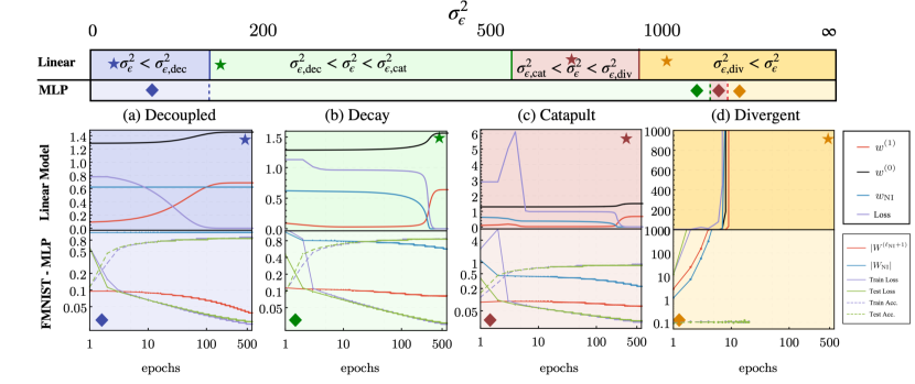
Figure 2: Evolution for a DNN with a NIN coupled to the first hidden layer, for two different models. Top bar: Regions for the phases as a function of the noise strength $\sigma_{\epsilon}$. The top darker shaded and bottom lighter shaded bar regions correspond to the linear and Multi-Layer Perceptron (MLP) models respectively. The stars and diamonds indicate the values of $\sigma_{\epsilon}$ used in the bottom plots. Top plots: Numerical solutions for the various phases of Eq. 5, describing the linear model. The data weights (black and red lines), NIW (blue) and loss functions (purple) are shown. In the decoupled and decay phases, data weights approach optimum values while the NIW decays slowly, whereas a larger noise magnitude results in a longer relaxation time. In the initial stages of the catapult phase no learning is achieved until the NIW sufficiently decays, when standard learning is resumed. In the divergent phase the system fails to learn, with breakdown after only a few epochs. Bottom plots: Various phases of NIW dynamics during training for a 1-hidden layer MLP with MSE loss and ReLU activations, trained on FMNIST. Solid (dashed) curves represent the loss (accuracy) values, for training (purple) and test (green) instances. The behavior displayed by the loss function, the NIWs (blue) and the subsequent layer weights (red) norms, corroborates the predictions of the linear model, discussed in Sec. 2. For experimental details, see App. B.

While non-linear, the solution to Eq. 5 is rather simple and is dictated by $\sigma_{\epsilon}$ and the initial conditions. We identify four different phases, demonstrated in Fig. 1 (right) and Fig. 2:

Decoupled phase.  When the scale of injected noise is sufficiently small, $\sigma_{\epsilon}\leq\sigma_{\epsilon,\rm{dec}}\equiv 2{\tilde{A}_{0}}/{\tilde{B}_{0}}$, the original optimization trajectory, driven by the $C_{t}$ term, is on average unaffected by the NIN, and the NIWs evolve according to a random walk, with step size dictated by the local gradient, $\tilde{A}_{t}$.

Decay phase.  For $\sigma_{\epsilon,\mathrm{dec}}^{2}<\sigma_{\epsilon}^{2}\ll\sigma_{\epsilon,\mathrm{cat}}^{2}\equiv\min[2/B_{0},2/\tilde{B}_{0}]$ the dynamics is initially dominated by the $\tilde{B}_{t}$ and $C_{t}$ terms, and as a consequence $w_{\mathrm{NI}}$ exponentially falls. Once $w_{\mathrm{NI}}$ is sufficiently small, the $A$-terms dominate and the dynamics is decoupled from the noise as in the previous phase.

The above two phases occur for rather small noise injection and, as discussed above, the noise is a mere small perturbation to the dynamics. However, for $\sigma_{\epsilon}>\sigma_{\epsilon,\rm cat}$, the equations become noise-dominated at initialization and the early dynamics becomes insensitive to the original learning objective. Early time evolution can then be understood by neglecting the $A$- and $C$-terms, and the equations become noise dominated at initialization, with the early times evolution entirely determined by $B_{t},\tilde{B}_{t}$ as

$$w^{(1)}_{t+1}=w^{(1)}_{t}(1-B_{t}\sigma_{\epsilon}^{2}),$$ (7)

$$w_{\rm{NI},t+1}=w_{\rm{NI},t}(1-\tilde{B}_{t}\sigma_{\epsilon}^{2}).$$

Consequently, the equations describe a DNN, trained using completely random data with no labels or learning objectives. The network evolution can then be separated into the following two distinct phases:

Catapult phase.  When $\sigma_{\epsilon,\mathrm{cat}}<\sigma_{\epsilon}<\sigma_{\epsilon,\mathrm{div}}\equiv\max(2/B_{0},2/\tilde{B}_{0})$, some, but not all, of the network weights begin diverging, as a stiff equation regime ensues due to the discrete nature of the SGD algorithm. Generally, this divergence can be driven by either the data or the NIWs, though in realistic scenarios the latter is more common and we therefore discuss for concreteness the $2/\tilde{B}_{0}<\sigma_{\epsilon}<2/B_{0}$ case. While the NIW (and the loss function) diverges, $w_{t}^{(1)}$ decays fast enough for the Hessian to be reduced, allowing for the network to recover, and resulting in a catapult effect. At this point the dynamics of the system behave similarly to the Decay Phase, albeit typically at a slower rate since the Hessian is now significantly smaller. These results are visible in Fig. 2(c).

Divergent phase. Once $\sigma_{\epsilon}^{2}\geq\sigma_{\epsilon,\rm{div}}^{2}$, the NIN overwhelms the network, and all weights (and loss function) diverge resulting in a failed training process. In non-linear networks, this phase can also occur if the second order perturbative approximation for the loss function breaks down.

While the discussion above pertained to a simplified scenario, it is expected to capture the features of the dynamics in the limit of large batch size $|\mathcal{B}|\to\infty$ and small noise variance $\sigma_{\epsilon}\ll 1$, as in this limit the second-order truncation of Eq. 2 is justified; we verify this numerically. The bottom row of Fig. 2 demonstrates the persistence of our predicted phase diagram for an over-parameterized DNN trained on the FMNIST dataset [28]. While the decoupled and decay phases occur for similar $\sigma_{\epsilon}$ values as those in the linear model, the large noise behavior is altered by the choice of non-linearities, loss function, batch size and number of layers. In particular, the noise variance values dictating the phase boundaries are somewhat different than those predicted by the linear model, however the existence of the boundaries themselves persists throughout our experiments. Some of these effects are partially explored in App. A.

4 Relating the Evolution of the NIWs and Loss

As discussed in Sec. 1, during the decay and catapult phases, the NIWs decay as the network attempts to learn, a phenomena which repeats both for re-randomized as well as fixed value NINs. Since the latter can be interpreted as the suppression of uncorrelated data features, understanding the relationship between the NIWs and loss evolutions could provide future insights regarding generalization.

Here, we take a step towards connecting the NIW dynamics with the loss dynamics, for the simple linear model, hinting that more complicated constructions could allow a more direct relationship between the two. With no NINs and for small enough learning rates,

$$\delta L^{(t+1)}=L^{(t+1)}-L^{(t)}\approx\frac{\partial L^{(t)}}{\partial\theta^{ij}}\left(\theta_{ij}^{(t+1)}-\theta_{ij}^{(t)}\right)=-\eta\left(\frac{\partial L^{(t)}}{\partial\theta^{ij}}\right)^{2}.$$ (8)

In the linear case, this simplifies to the trace of the global Hessian, multiplied by the loss, as shown in App. D. We demonstrate that a similar behavior holds for a realistic DNN in Fig. 1(center, right).

To show how this relates to the noise node, it is easier (though not necessary) to take the continuous time limit ($\eta\to 0$) of Eq. 5 resulting in a set of coupled Langevin equations [29]. In App. D, we show that if we can neglect the effect of the NIN on the loss, the solution of the full continuous time equations leads to the following relations

$$L_{\epsilon=0}(t) \sim L_{\epsilon=0}(0)e^{-2\sigma_{x}^{2}\int_{0}^{t}\left[(w^{(0)}(t^{\prime}))^{2}+(w^{(1)}(t^{\prime}))^{2}\right]dt^{\prime}},$$ (9)

$$w_{\mathrm{NI}}(t) \sim e^{-\sigma_{\epsilon}^{2}\int_{0}^{t}(w^{(1)}(t^{\prime}))^{2}dt^{\prime}}.$$

We define the two time scales

$$\tau_{\mathrm{noise}}=-w_{\mathrm{NI}}/\dot{w}_{\mathrm{NI}}|_{t=0},\qquad\leavevmode\nobreak\ \tau_{\mathrm{loss}}=-L_{\epsilon=0}/\dot{L}_{\epsilon=0}|_{t=0},$$ (10)

which differ both by a multiplicative factor and by the magnitude of the weight connecting the input with the first layer. The first comes from the difference between data and noise distributions, while the second is due to the NINs being connected at the same layer as the input ($\ell_{\mathrm{NI}}=0$), such that the local Hessian which controls their evolution is insensitive to first layer contributions to the loss evolution. Adding multiple NINs in more complicated constructions which would be sensitive to the input layer’s weights could provide a novel probe for how various local parts of the Hessian affect the evolution of loss functions.

5 Conclusions

The study of the relations between training dynamics and learning capabilities of DNNs via the injection of noise through optimizable connections provides a novel path toward interpretable deep learning. In the future, NINs could have many possible technological applications. For instance, one could recognize the evolution of NIWs among regular data weights to identify features which are uncorrelated with the labels, and thus build normalization schemes [30, 31, 32, 33, 34] to suppress such weights in an effort to tackle internal covariate shift. Furthermore, it’s possible that by observing the evolution of the NIWs one could learn more about how the different parts of the DNN affect the evolution of the loss, as well as possibly teach one about generalization, as the NIWs cannot be memorized by the network, only suppressed. Specifically, landing in different points on the loss landscape as a result of noise mitigation could inform us on the possible relation between loss curvature and noise resistant networks. While this early study clearly shows that our analytical understanding captures at least some features of NIN dynamics, more complicated architectures are expected to have much richer structure and thus more complex evolution. For example, bounded nonlinearities cannot generate a divergence in the loss function, implying a different behavior during the catapult and divergent phases. There is also a clear interplay with the network hyperparameters — a small batch size increases the effect of the stochastic gradient, while changing the learning rate can change the boundaries of the phases. Analytical studies of other DNNs, including convolutional, recurrent, and transformer architectures, could identify analogous probes for techniques deployed at industry scale.

Appendix A Additional Empirical Results

Here, we present additional results not included in the main text.

In Fig. 3 below, we show the different phases predicted in Sec. 2, for a 3 layer MLP with ReLU activations, trained on FMNIST using cross-entropy (CE) loss. These results are similar to the ones obtained for a network which was trained using the MSE loss, shown in Fig. 2(bottom), demonstrating the persistence of the phase structure regardless of the loss function.

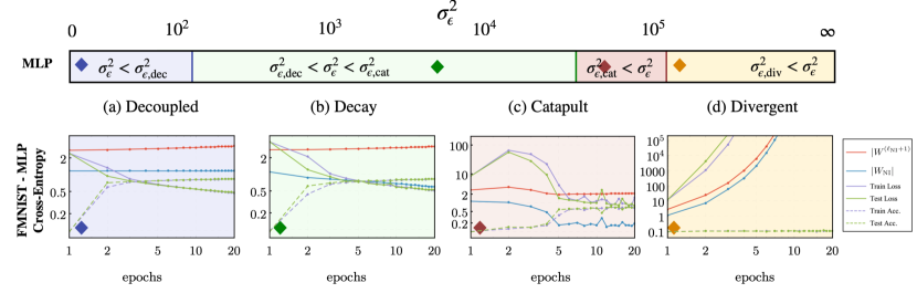
Figure 3: Dynamical evolution of a network with a NIN coupled to the first hidden layer of a DNN. Top bar: The light shaded regions separating the four phases as a function of the noise strength, $\sigma_{\epsilon}$. The colored diamonds indicate the values of $\sigma_{\epsilon}$ used in the bottom plots. Bottom plots: Various phases of the NIW dynamics during training for a 1-hidden layer MLP with Cross-Entropy loss and ReLU activations, trained on the full FMNIST dataset. The data weights (black and red lines), NIW (blue) and loss functions (purple) are shown. In the decoupled and decay phases, data weights approach optimum values while the NIW decays slowly. Larger noise implies longer time for this process to end. In the initial stages of the catapult phase no learning is achieved until the NIW sufficiently decays, when standard learning is resumed. Lastly, in the divergent phase the system fails to learn, reaching a breakdown after only a few epochs. Solid (dashed) curves represent the loss (accuracy) values, for training (violate) and test (green) instances. The behavior displayed by the loss function, the norms of the NIWs (blue) and the weights connected to the subsequent layer (red), corroborates the predictions of the linear model, as well as the results obtained on the same network, trained using an MSE loss function, discussed in Sec. 2. For experimental details, see App. B.

Appendix B Experimental Details

In the main text we present results for models trained on the Fashion-MINST (FMNIST) dataset [28]. FMNIST contains 70,000 grayscale images in 10 categories. The images show individual articles of clothing at low resolution ($28\times 28$ pixels). We preprocess the data by subtracting the mean and dividing by the variance of the training data, and train using a $60/40$ training/validation split. All test accuracy evaluations are done with the NIN output set to $0$, i.e., $\epsilon=0$.

Implementation Details : For all of our experiments, we utilize a Multi-Layer Perceptron (MLP).

We optimize using vanilla SGD with either MSE or Sparse Cross-Entropy loss. The model parameters $\boldsymbol{\theta},\boldsymbol{w}_{\rm{NI}}$ are initialized at iteration $t=0$ using a normal distribution as $\boldsymbol{w}_{0},\boldsymbol{w}_{\rm{NI},0}=1/\sqrt{N_{\mathrm{fan-in}}}$ unless otherwise specified.

Here we describe experimental settings specific to a figure.

Figure 1. Fully connected, 3 hidden layers, $N_{w}=1024$, ReLU non-linearity trained using SGD (no momentum) on FMNIST using a Sparse-Cross-Entropy loss function. Batch size = 128, with learning rate $\eta=0.05$, using weight normalization $w^{(\ell)}\sim\mathcal{N}(0,1/d_{\ell}),b=0$. The hyperparameters are chosen to obtain good generalization performance without a NIN.

Figure 2. (top row): Numerical solution of Eq. 5. Learning rate set at $\eta=0.01$. Intialization values for the weights were chosen to mimic a standard over-parameterized regime, i.e. $w^{(0)},w_{\rm{NI}}^{(0)}\sim\mathcal{N}(0,1)$, while $w^{(0)},w_{\rm{NI}}^{(0)}\sim\mathcal{N}(0,1/100)$. The target is the identity, i.e. $M=1$, as the equations are invariant under reparameterization with respect to $M$. The only values of consequence are then the ratios of weights at initialization and the learning rate. Therefore the actual values of the learning rate and noise variance are chosen to make the effects visible to the eye for a short training period but do not affect the final results in any way.

Figure 2 (bottom row), Fig. 3. Fully connected, one hidden layer $N_{w}=1024$, ReLU non-linearity trained using SGD (no momentum) on FMNIST. Batch size = 1000, with learning rate $\eta=0.01$, using weight normalization $W^{(\ell)}\sim\mathcal{N}(0,1/d_{\ell}),b=0$. The hyperparameters are chosen to obtain good generalization performance without a NIN.

In Fig. 2(bottom) and Fig. 3 we use different loss functions, namely, MSE and Cross-Entropy, respectively. We detail the amount of noise injection used in each of the two figures in Table 1.

	Decoupled ($\sigma_{\epsilon}^{2}$)	Decay ($\sigma_{\epsilon}^{2}$)	Catapult ($\sigma_{\epsilon}^{2}$)	Divergent ($\sigma_{\epsilon}^{2}$)
MSE	$10^{-4}\cdot d_{\rm{Input}}/(N_{w}\eta)$	$30\cdot d_{\rm{Input}}/(N_{w}\eta)$	$47\cdot d_{\rm{Input}}/(N_{w}\eta)$	$50\cdot d_{\rm{Input}}/(N_{w}\eta)$
CE	$10^{-4}\cdot d_{\rm{Input}}/\eta$	$0.1\cdot d_{\rm{Input}}/\eta$	$d_{\rm{Input}}/\eta$	$1.8\cdot d_{\rm{Input}}/\eta$

Table 1: Noise injection strength ($\sigma_{\epsilon}^{2}$) used in Fig. 2(bottom), denoted as MSE, and Fig. 3, denoted as CE.

Appendix C Further Details On the Noise Parameter Expansion

Here we provide additional details on the theoretical analysis of the general model in Sec. 2. Starting with the noise translated loss function

$$L({\boldsymbol{\theta}},{W_{\mathrm{NI}}}) =\frac{1}{|\mathcal{B}|}\sum_{\{\boldsymbol{x},\epsilon,\boldsymbol{y}\}\in\mathcal{B}}\mathcal{L}(\boldsymbol{\theta},{W_{\rm{NI}}};{\boldsymbol{x}},\epsilon,\boldsymbol{y})=\frac{1}{|\mathcal{B}|}\sum_{\{\boldsymbol{x},\epsilon,\boldsymbol{y}\}\in\mathcal{B}}e^{\epsilon{W^{T}_{\rm{NI}}}\nabla_{{\boldsymbol{z}}^{(\ell_{\rm NI})}}}\mathcal{L}(\boldsymbol{\theta};{\boldsymbol{x}},\boldsymbol{y})$$

$$=L({\boldsymbol{\theta}})+\frac{1}{|\mathcal{B}|}\sum_{\begin{subarray}{c}\{\boldsymbol{x},\epsilon,\boldsymbol{y}\}\\ \in\mathcal{B}\end{subarray}}\sum_{k=1}^{\infty}\frac{1}{k!}(\epsilon{W^{T}_{\rm{NI}}}\cdot\nabla_{{\boldsymbol{z}^{(\ell_{\rm{NI}})}}})^{k}\mathcal{L}(\boldsymbol{\theta};{\boldsymbol{x}},\epsilon,{\boldsymbol{y}}).$$

Expanding in powers of $\epsilon{W_{\rm{NI}}}$, we obtain an infinite series given by

$$L({\boldsymbol{\theta}},{W_{\rm{NI}}})=L({\boldsymbol{\theta}})+\frac{1}{|\mathcal{B}|}\sum_{\{\boldsymbol{x},\epsilon,\boldsymbol{y}\}\in\mathcal{B}}\sum_{k=1}^{\infty}\frac{1}{k!}(\epsilon{W^{T}_{\rm{NI}}}\cdot\nabla_{{\boldsymbol{z}^{(\ell_{\rm{NI}})}}})^{k}\mathcal{L}(\boldsymbol{\theta};{\boldsymbol{x}},\epsilon,{\boldsymbol{y}}).$$ (11)

Performing the batch averaging explicitly amounts to averaging over the statistics of the data and noise, resulting in the loss

$$\langle\mathcal{L}(\boldsymbol{\theta},W_{\rm{NI}})\rangle=\langle\mathcal{L}(\boldsymbol{\theta})\rangle+W^{T}_{\rm{NI}}\cdot\langle{\epsilon}\boldsymbol{\textsl{g}}_{\ell_{\rm{NI}}}\rangle+\frac{1}{2}{W}_{\rm{NI}}^{T}\langle\epsilon^{2}\mathcal{H}_{\ell_{\rm{NI}}}\rangle{W}_{\rm{NI}}+\ldots$$ (12)

Here, batch averaging is denoted by $\langle..\rangle$, the local gradient is ${\boldsymbol{\textsl{g}}}_{\ell_{\rm{NI}}}=\nabla_{{\boldsymbol{z}}^{(\ell_{\rm{NI}})}}\mathcal{L}({\boldsymbol{\theta}};{\boldsymbol{x}},{\boldsymbol{y}})$ and Hessian ${{\mathcal{H}_{\ell_{\rm{NI}}}}}={\nabla_{\boldsymbol{z}^{(\ell_{\rm{NI}})}}\nabla^{T}_{\boldsymbol{z}^{(\ell_{\rm{NI}})}}}\mathcal{L}(\boldsymbol{\theta};\boldsymbol{x},\boldsymbol{y})$ are network-dependent functions, pertaining to the NIN layer.

Taking $\epsilon$ sampled from a distribution with zero mean, the local gradient and Hessian contributions simplify as $\langle\epsilon{\boldsymbol{\textsl{g}}}_{\ell_{\rm{NI}}}\rangle\sim\sqrt{\langle{\boldsymbol{\textsl{g}}}_{\ell_{\rm{NI}}}^{2}\rangle}\Phi\sigma_{\epsilon}/\sqrt{|\mathcal{B}|}$, where $\langle{\boldsymbol{\textsl{g}}}_{\ell_{\rm{NI}}}^{2}\rangle$ is the vector of the batch-averaged absolute value of the gradient and $\Phi$ is a random variable with mean $0$ and variance $1$, and $\langle\epsilon^{2}\mathcal{H}_{\ell_{\mathrm{NI}}}\rangle\sim\sigma_{\epsilon}^{2}\langle\mathcal{H}_{\ell_{\rm{NI}}}\rangle$, where we define $\sigma^{2}_{\epsilon}\equiv\langle\epsilon^{2}\rangle$ as the variance of the injected noise.

This result, as proven below, makes explicit that odd terms in the expansion are suppressed by $|\mathcal{B}|^{-1/2}$.

The last step in the derivation is performed by taking the SGD update step with respect to the NIWs, which is simply

$$W_{\rm{NI}}^{(t+1)}=W_{\rm{NI}}^{(t)}-\eta\frac{\partial L(\boldsymbol{\theta}^{(t)},W_{\rm{NI}}^{(t)})}{\partial W_{\rm{NI}}^{(t)}}.$$ (13)

Finally, utilizing Eq. 12 we arrive at

$$W_{\rm{NI}}^{(t+1)}=W_{\rm{NI}}^{(t)}-\eta\frac{\sigma_{\epsilon}\Phi}{\sqrt{|\mathcal{B}|}}\sqrt{\langle(\boldsymbol{\textsl{g}}_{\ell_{\rm{NI}}}^{(t)})^{2}\rangle}-\frac{\eta\sigma^{2}_{\epsilon}}{2}\left\langle\mathcal{H}_{\ell_{\rm{NI}}}^{(t)}\right\rangle W_{\rm{NI}}^{(t)}+\dots,$$ (14)

which is given in the main text as Eq. 2.

We now turn to discuss our estimation of batch-averaged terms which are proportional to powers of $\epsilon$. Generically, such terms can be written as $q\epsilon^{n}$, where $n$ is an integer, and $q$ is some sample-dependent variable, possibly with other indices.

The goal of this appendix is to prove the following theorem:

Theorem 1.

Let q be a sample-dependent variable, with a finite mean $\langle q\rangle$ and with $Q\equiv\sqrt{\langle q^{2}\rangle}$. And let $\epsilon$ be the output of some NIN, which has a PDF symmetric around zero (and consequentially of zero mean), and for some integer $n$, $\langle\epsilon^{n}\rangle=(\sigma_{n,\epsilon})^{n}$, and $\langle\epsilon^{2n}\rangle=(\sigma_{2n,\epsilon})^{2n}$. For such a case, the average of $q\epsilon^{n}$ over a batch ${\mathcal{B}}$ has a mean of $\langle q\rangle(\sigma_{n,\epsilon})^{n}$, and a variance of $\left(\sigma_{2n,\epsilon}^{2n}Q^{2}-\langle q\rangle^{2}\sigma_{n,\epsilon}^{2n}\right)/\sqrt{|B|}$.

For odd $n$s, this simplifies to having zero mean, and a standard deviation of $Q\sigma_{2n,\epsilon}^{n}/\sqrt{|\mathcal{B}|}$.

We note that this theorem is the reasoning for the estimate $|\left\langle q\epsilon^{n}\right\rangle_{\mathcal{B}}|\sim\mathcal{O}(1)(\sigma_{\epsilon,2n})^{n}Q/\sqrt{|\mathcal{B}|}$ for odd $n$s, as well as the estimate of $\left\langle q\epsilon^{n}\right\rangle_{\mathcal{B}}\approx\sigma_{n,\epsilon}^{2n}\left\langle q\right\rangle$, for an even $n$ and a large enough $|\mathcal{B}|$. We also note that for a large enough $|\mathcal{B}|$, this theorem immediately follows from the law of large numbers, however we prove it for any $|\mathcal{B}|$.

Proof.

We can see that for a single term, and the average over the entire distribution

$$\left\langle q\epsilon^{n}\right\rangle=\left\langle q\right\rangle\left\langle\epsilon^{n}\right\rangle.$$ (15)

This is due to the fact that $\epsilon$ is a random output that is independent of $q$, and thus $\langle q\epsilon^{n}\rangle=\langle q\rangle\langle\epsilon^{n}\rangle$. For an odd $n$, this is simply equal to 0, since $\epsilon$’s PDF is symmetric around zero, so for odd $n$s, $\langle\epsilon^{n}\rangle=0$.

Similarly, we may note that

$${\rm Var}(q\epsilon^{n})=\left\langle(q\epsilon^{n})^{2}-\left\langle(q\epsilon^{n})\right\rangle^{2}\right\rangle=Q^{2}\sigma_{\epsilon,n}^{2n}-\langle q\rangle\langle\epsilon^{n}\rangle.$$ (16)

Where we once again use the independence of $q$ and $\epsilon$, and this time also use the definitions of $Q$ and $\sigma_{\epsilon,n}$.

We can now see that

$$\left\langle\left\langle q\epsilon^{n}\right\rangle_{\mathcal{B}}\right\rangle=\frac{1}{|\mathcal{B}|}\left\langle\sum_{i=1}^{|\mathcal{B}|}q_{i}\epsilon_{i}^{n}\right\rangle=\frac{1}{|\mathcal{B}|}\sum_{i=1}^{|\mathcal{B}|}\left\langle q\epsilon^{n}\right\rangle=\langle q\rangle\langle\epsilon^{n}\rangle,$$ (17)

and similarly,

$${\rm Var}\left(\left\langle q\epsilon^{n}\right\rangle_{\mathcal{B}}\right)=\left\langle\left\langle q\epsilon^{n}\right\rangle_{\mathcal{B}}^{2}-\left\langle q\epsilon^{n}\right\rangle_{\mathcal{B}}^{2}\right\rangle.$$ (18)

We have already computed the second term, so now let us compute the first one,

$$\left\langle\left\langle q\epsilon^{n}\right\rangle_{\mathcal{B}}^{2}\right\rangle=\frac{1}{|\mathcal{B}|^{2}}\left\langle\sum_{j=1}^{|\mathcal{B}|}\sum_{i=1}^{|\mathcal{B}|}(q_{j}\epsilon_{j}^{n})(q_{i}\epsilon_{i}^{n})\right\rangle=\frac{1}{|\mathcal{B}|}\left\langle q^{2}\epsilon^{2n}\right\rangle+\frac{1}{|\mathcal{B}|^{2}}\left\langle\sum_{j=1}^{|\mathcal{B}|}\sum_{i=1,i\neq j}^{|\mathcal{B}|}(q_{j}\epsilon_{j}^{n})(q_{i}\epsilon_{i}^{n})\right\rangle$$ (19)

, where we divided the two sums to the contribution from $i=j$ and the contribution from $i\neq j$. The second term in Eq. (19) is simply $|\mathcal{B}|^{2}-|\mathcal{B}|$ times the same term, and is therfore equal to,

$$\frac{1}{|\mathcal{B}|^{2}}\left\langle\sum_{j=1}^{|\mathcal{B}|}\sum_{i=1,i\neq j}^{|\mathcal{B}|}(q_{j}\epsilon_{j}^{n})(q_{i}\epsilon_{i}^{n})\right\rangle=\frac{|\mathcal{B}|^{2}-|\mathcal{B}|}{|\mathcal{B}|^{2}}\left\langle(q_{j}\epsilon_{j}^{n})(q_{i}\epsilon_{i}^{n})\right\rangle_{i\neq j}.$$ (20)

We assume there is an arbitrarily large space of samples, which we may name as $\mathcal{A}$. Let us write its size as $|\mathcal{A}|$, and assume that $|\mathcal{A}|\to\infty$ and therefore,

$$\left\langle(q_{j}\epsilon_{j}^{n})(q_{i}\epsilon_{i}^{n})\right\rangle_{i\neq j} =\frac{1}{|\mathcal{A}|}\sum_{i,j\in\mathcal{A},i\neq j}(q_{j}\epsilon_{j}^{n})(q_{i}\epsilon_{i}^{n})=\frac{1}{|\mathcal{A}|^{2}}\sum_{i,j\in\mathcal{A}}(q_{j}\epsilon_{j}^{n})(q_{i}\epsilon_{i}^{n})-\frac{1}{|\mathcal{A}|^{2}}\sum_{j\in\mathcal{A}}(q_{j}\epsilon_{j}^{n})^{2}$$ (21)

$$=\left\langle q\epsilon^{n}\right\rangle^{2}-\frac{1}{|\mathcal{A}|}\left\langle(q\epsilon^{n})\right\rangle=\left\langle q\epsilon^{n}\right\rangle^{2},$$

where in the last equality we used $|\mathcal{A}|\to\infty$. We can now write the variance of the batch averaged quantity, by collecting all the different terms, and find tha

$${\rm Var}\left(\left\langle q\epsilon^{n}\right\rangle_{\mathcal{B}}\right)=\frac{1}{|\mathcal{B}|}\left(\left\langle q^{2}\epsilon^{2n}\right\rangle-\left\langle q\epsilon^{n}\right\rangle^{2}\right),$$ (22)

as originally postulated. ∎

Appendix D Decay Time-scale Derivation

Here, we derive the timescale for the NIW to decay, while the loss converges to its minimum, for the linear example given in Sec. 2.

Assuming that the system is in the decay phase, i.e. the SGD equations are given by

$$w^{(1)}_{t+1} =w^{(1)}_{t}-\eta(w^{(1)}_{t}w^{(0)}_{t}-M)w^{(0)}_{t}\sigma_{x}^{2},$$ (23)

$$w_{\mathrm{NI},t+1} =w_{\mathrm{NI},t}(1-\eta(w^{(1)}_{t})^{2}\sigma_{\epsilon}^{2}).$$ (24)

Since the noise injection does not cause the system to diverge at this stage, the continuous time limit ($\eta\to 0$) is expected to hold, simplifying the equations as

$$\dot{w}^{(1)} =-(w^{(1)}w^{(0)}-M)w^{(0)}\sigma_{x}^{2},$$ (25)

$$\dot{w}_{\mathrm{NI}} =-(w^{(1)})^{2}\sigma_{\epsilon}^{2}{w}_{\mathrm{NI}},$$ (26)

where it is implied that all weights are functions of time, $w=w(t)$. Next, we can define the loss function in the absence of noise, which will be the quantity we wish to track. This function is simply

$$L=\frac{1}{2}\left((w^{(1)}w^{(0)}-M)\sigma_{x}\right)^{2},$$ (27)

which results in the continuous time update equation for the loss and the data weights

$$\dot{L} =\sigma_{x}^{2}\left((w^{(1)}w^{(0)}-M)\right)\left(\dot{w}^{(1)}w^{(0)}+\dot{w}^{(0)}w^{(1)}\right)=\sigma_{x}\sqrt{2L}\left(\dot{w}^{(1)}w^{(0)}+\dot{w}^{(0)}w^{(1)}\right),$$ (28)

$$\dot{w}^{(1)} =-{\rm{sign}}(w^{(1)}w^{(0)}-M)\sqrt{2L}\sigma_{x}w^{(0)},\quad\dot{w}^{(0)}=-{\rm{sign}}(w^{(1)}w^{(0)}-M)\sqrt{2L}\sigma_{x}w^{(1)},$$ (29)

combining these equations we obtain for the loss function and the NIW we have

$$\dot{L} =-2\sigma_{x}^{2}\left((w^{(0)})^{2}+(w^{(1)})^{2}\right)L,$$ (30)

$$\dot{w}_{\mathrm{NI}} =-\sigma_{\epsilon}^{2}(w^{(1)})^{2}{w}_{\mathrm{NI}},$$ (31)

where we identify that the loss function evolves according to the trace of the full Hessian $\operatorname{Tr}{(H_{\boldsymbol{\theta}})}=\sigma_{x}^{2}\left((w^{(0)})^{2}+(w^{(1)})^{2}\right)$, while the NIW evolves according to the trace of the local Hessian $\operatorname{Tr}{(\mathcal{H}_{z})}=(w^{(1)})^{2}$.

These equations imply an exponential evolution for both the loss function and the NIW. The relevant timescales can be read by integrating the equations, hence

$$L(t) \sim e^{-2\sigma_{x}^{2}\int_{0}^{t}\left((w^{(0)}(t^{\prime}))^{2}+(w^{(1)}(t^{\prime}))^{2}\right)dt^{\prime}},$$ (32)

$$w_{\mathrm{NI}}(t) \sim e^{-\sigma_{\epsilon}^{2}\int_{0}^{t}(w^{(1)}(t^{\prime}))^{2}dt^{\prime}}.$$ (33)

as presented in the main text.

References

• Hochreiter and Schmidhuber [1997] Sepp Hochreiter and Jürgen Schmidhuber. Flat minima. Neural computation, 9(1):1–42, 1997.
• Sagun et al. [2016] Levent Sagun, Leon Bottou, and Yann LeCun. Eigenvalues of the hessian in deep learning: Singularity and beyond. arXiv preprint arXiv:1611.07476, 2016.
• Gur-Ari et al. [2018] Guy Gur-Ari, Daniel A. Roberts, and Ethan Dyer. Gradient descent happens in a tiny subspace, 2018. URL https://arxiv.org/abs/1812.04754.
• Ghorbani et al. [2019] Behrooz Ghorbani, Shankar Krishnan, and Ying Xiao. An investigation into neural net optimization via hessian eigenvalue density. In International Conference on Machine Learning, pages 2232–2241. PMLR, 2019.
• Yao et al. [2020] Zhewei Yao, Amir Gholami, Kurt Keutzer, and Michael W Mahoney. Pyhessian: Neural networks through the lens of the hessian. In 2020 IEEE international conference on big data (Big data), pages 581–590. IEEE, 2020.
• Papyan [2018] Vardan Papyan. The full spectrum of deepnet hessians at scale: Dynamics with sgd training and sample size. arXiv preprint arXiv:1811.07062, 2018.
• Li et al. [2020] Xinyan Li, Qilong Gu, Yingxue Zhou, Tiancong Chen, and Arindam Banerjee. Hessian based analysis of sgd for deep nets: Dynamics and generalization. In Proceedings of the 2020 SIAM International Conference on Data Mining, pages 190–198. SIAM, 2020.
• Zhang et al. [2016] Chiyuan Zhang, Samy Bengio, Moritz Hardt, Benjamin Recht, and Oriol Vinyals. Understanding deep learning requires rethinking generalization. CoRR, abs/1611.03530, 2016. URL http://arxiv.org/abs/1611.03530.
• Graves [2011] Alex Graves. Practical variational inference for neural networks. Advances in neural information processing systems, 24, 2011.
• Ba and Frey [2013] Jimmy Ba and Brendan Frey. Adaptive dropout for training deep neural networks. Advances in neural information processing systems, 26:3084–3092, 2013.
• Goodfellow et al. [2013] Ian J Goodfellow, Dumitru Erhan, Pierre Luc Carrier, Aaron Courville, Mehdi Mirza, Ben Hamner, Will Cukierski, Yichuan Tang, David Thaler, Dong-Hyun Lee, et al. Challenges in representation learning: A report on three machine learning contests. In International conference on neural information processing, pages 117–124. Springer, 2013.
• Srivastava et al. [2014] Nitish Srivastava, Geoffrey Hinton, Alex Krizhevsky, Ilya Sutskever, and Ruslan Salakhutdinov. Dropout: a simple way to prevent neural networks from overfitting. The journal of machine learning research, 15(1):1929–1958, 2014.
• Wan et al. [2013] Li Wan, Matthew Zeiler, Sixin Zhang, Yann Le Cun, and Rob Fergus. Regularization of neural networks using dropconnect. In International conference on machine learning, pages 1058–1066. PMLR, 2013.
• Kang et al. [2016] Guoliang Kang, Jun Li, and Dacheng Tao. Shakeout: A new regularized deep neural network training scheme. In Thirtieth AAAI Conference on Artificial Intelligence, 2016.
• Wager et al. [2013] Stefan Wager, Sida Wang, and Percy S Liang. Dropout training as adaptive regularization. Advances in neural information processing systems, 26:351–359, 2013.
• Li and Liu [2018] Yinan Li and Fang Liu. Whiteout: Gaussian adaptive noise regularization in deep neural networks, 2018.
• Li and Liu [2020] Yinan Li and Fang Liu. Adaptive gaussian noise injection regularization for neural networks. In Min Han, Sitian Qin, and Nian Zhang, editors, Advances in Neural Networks – ISNN 2020, pages 176–189, Cham, 2020. Springer International Publishing. ISBN 978-3-030-64221-1.
• Dhifallah and Lu [2021] Oussama Dhifallah and Yue M. Lu. On the inherent regularization effects of noise injection during training, 2021. URL https://arxiv.org/abs/2102.07379.
• Blanc et al. [2020] Guy Blanc, Neha Gupta, Gregory Valiant, and Paul Valiant. Implicit regularization for deep neural networks driven by an Ornstein–Uhlenbeck like process. In Conference on learning theory, pages 483–513. PMLR, 2020.
• Damian et al. [2021] Alex Damian, Tengyu Ma, and Jason D Lee. Label noise SDG provably prefers flat global minimizers. Advances in Neural Information Processing Systems, 34:27449–27461, 2021.
• HaoChen et al. [2021] Jeff Z HaoChen, Colin Wei, Jason Lee, and Tengyu Ma. Shape matters: Understanding the implicit bias of the noise covariance. In Conference on Learning Theory, pages 2315–2357. PMLR, 2021.
• Li et al. [2021] Zhiyuan Li, Tianhao Wang, and Sanjeev Arora. What happens after SGD reaches zero loss? -a mathematical framework. CoRR, abs/2110.06914, 2021. URL https://arxiv.org/abs/2110.06914.
• Pillaud-Vivien et al. [2022] Loucas Pillaud-Vivien, Julien Reygner, and Nicolas Flammarion. Label noise (stochastic) gradient descent implicitly solves the lasso for quadratic parametrisation, 2022. URL https://arxiv.org/abs/2206.09841.
• Thomas et al. [2020] Valentin Thomas, Fabian Pedregosa, Bart Merriënboer, Pierre-Antoine Manzagol, Yoshua Bengio, and Nicolas Le Roux. On the interplay between noise and curvature and its effect on optimization and generalization. In International Conference on Artificial Intelligence and Statistics, pages 3503–3513. PMLR, 2020.
• Roberts [2021] Daniel A Roberts. SGD implicitly regularizes generalization error. arXiv preprint arXiv:2104.04874, 2021.
• Gunasekar et al. [2018] Suriya Gunasekar, Jason Lee, Daniel Soudry, and Nathan Srebro. Implicit bias of gradient descent on linear convolutional networks, 2018. URL https://arxiv.org/abs/1806.00468.
• Lewkowycz et al. [2020] Aitor Lewkowycz, Yasaman Bahri, Ethan Dyer, Jascha Sohl-Dickstein, and Guy Gur-Ari. The large learning rate phase of deep learning: the catapult mechanism, 2020.
• Xiao et al. [2017] Han Xiao, Kashif Rasul, and Roland Vollgraf. Fashion-MNIST: a novel image dataset for benchmarking machine learning algorithms, 2017.
• Lemons and Gythiel [1997] Don S. Lemons and Anthony Gythiel. Paul langevin’s 1908 paper “on the theory of brownian motion” [“sur la théorie du mouvement brownien,” c. r. acad. sci. (paris) 146, 530–533 (1908)]. American Journal of Physics, 65(11):1079–1081, 1997. doi: 10.1119/1.18725. URL https://doi.org/10.1119/1.18725.
• Ioffe and Szegedy [2015] Sergey Ioffe and Christian Szegedy. Batch normalization: Accelerating deep network training by reducing internal covariate shift. In ICML, 2015.
• Arpit et al. [2016] Devansh Arpit, Yingbo Zhou, Bhargava U. Kota, and Venu Govindaraju. Normalization propagation: A parametric technique for removing internal covariate shift in deep networks, 2016. URL https://arxiv.org/abs/1603.01431.
• Hoffer et al. [2018] Elad Hoffer, Ron Banner, Itay Golan, and Daniel Soudry. Norm matters: efficient and accurate normalization schemes in deep networks. In NeurIPS, 2018.
• Schneider et al. [2020] Steffen Schneider, Evgenia Rusak, Luisa Eck, Oliver Bringmann, Wieland Brendel, and Matthias Bethge. Improving robustness against common corruptions by covariate shift adaptation. ArXiv, abs/2006.16971, 2020.
• Xu et al. [2021] Renzhe Xu, Peng Cui, Zheyan Shen, Xingxuan Zhang, and Tong Zhang. Why stable learning works? a theory of covariate shift generalization. ArXiv, abs/2111.02355, 2021.