Causal Explanation for Reinforcement Learning:
Quantifying State and Temporal Importance

Abstract

Explainability plays an increasingly important role in machine learning. Furthermore, humans view the world through a causal lens and thus prefer causal explanations over associational ones. Therefore, in this paper, we develop a causal explanation mechanism that quantifies the causal importance of states on actions and such importance over time. We also demonstrate the advantages of our mechanism over state-of-the-art associational methods in terms of RL policy explanation through a series of simulation studies, including crop irrigation, Blackjack, collision avoidance, and lunar lander.

1 Introduction

Reinforcement learning (RL) is increasingly being considered in domains with significant social and safety implications such as healthcare, transportation, and finance. This growing societal-scale impact has raised a set of concerns, including trust, bias, and explainability. For example, can we explain how an RL agent arrives at a certain decision? When a policy performs well, can we explain why? These concerns mainly arise from two factors. First, many popular RL algorithms, particularly deep RL, utilize neural networks, which are essentially black boxes with their inner workings being opaque not only to lay persons but also to data scientists. Second, RL is a trial-and-error learning algorithm in which an agent tries to find a policy that minimizes a long-term reward by repeatedly interacting with its environment. Temporal information such as relationships between states at different time instances plays a key role in RL and subsequently adds another layer of complexity compared to supervised learning.

The field of explainable RL (XRL), a sub-field of explainable AI (XAI), aims to partially address these concerns by providing explanations as to why an RL agent arrives at a particular conclusion or action. While still in its infancy, XRL has made good progress over the past few years, particularly by taking advantage of existing XAI methods (Puiutta and Veith 2020; Heuillet, Couthouis, and Díaz-Rodríguez 2021; Wells and Bednarz 2021). For instance, inspired by the saliency map method (Simonyan, Vedaldi, and Zisserman 2014) in supervised learning which explains image classifiers by highlighting “important” pixels in terms of classifying images, some XRL methods attempt to explain the decisions made by an RL agent by generating maps that highlight “important” state features (Iyer et al. 2018; Greydanus et al. 2018; Mott et al. 2019). However, there exist at least two major limitations in state-of-the-art XRL methods. First, the majority of them take an associational perspective. For instance, the aforementioned studies quantify the “importance” of a feature by calculating the correlation between the state feature and an action. Since it is well known that “correlation doesn’t imply causation” (Pearl 2009), it is possible that features with a high correlation may not necessarily be the real “cause” of the action, resulting in a misleading explanation that can lead to user skepticism and possibly even rejection of the RL system. Second, temporal information is not generally considered. Temporal effects, such as the interaction between states and actions over time, which as mentioned previously is essential in RL, are not taken into account.

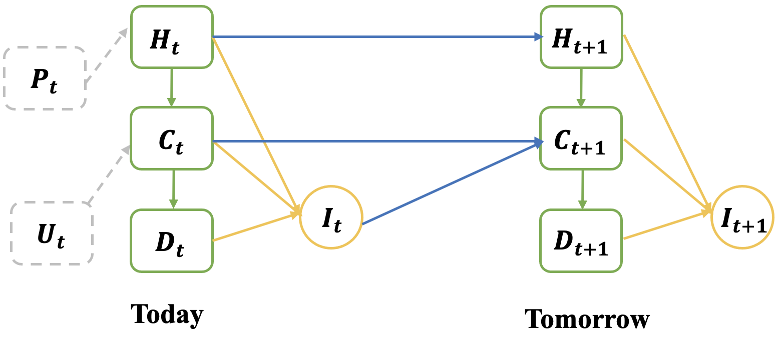
Figure 1: Causal graph of the crop irrigation problem. Endogenous and exogenous states are denoted by dashed and solid rectangles, respectively, while actions are denoted by circles. More details about causal graphs can be found in the Preliminaries section.

In this paper, we propose a causal XRL mechanism. Specifically, we explain an RL policy by incorporating a causal model that we have about the relationship between states and actions. To best illustrate the key features of our XRL mechanism, we use a concrete crop irrigation problem as an example, as shown in Fig. 1 (more details can be found in the Evaluation section). In this problem, an RL policy $\pi$ controls the amount of irrigation water ($I_{t}$) based on the following endogenous (observed) state variables: humidity ($H_{t}$), crop weight ($C_{t}$), and radiation ($D_{t}$). Its goal is to maximize the crop yield during harvest. Crop growth is also affected by some other features, including the observed precipitation ($P_{t}$) and other exogenous (unobserved) variables $U_{t}$. To explain why policy $\pi$ arrives at a particular action $I_{t}$ at the current state, our XRL method quantifies the causal importance of each state feature, such as $H_{t}$, in the context of this action $I_{t}$ via counterfactual reasoning (Byrne 2019; Miller 2019), i.e., by calculating how the action would have changed if the feature had been different.

Our proposed XRL mechanism addresses the aforementioned limitations as follows. First, our method can generate inherently causal explanations. To be more specific, in essence, importance measures used in associational methods can only capture direct effects while our causal importance measures capture total causal effects. For example, for the state feature $H_{t}$, our method can account for two causal chains: the direct effect chain $H_{t}\to I_{t}$ and the indirect effect chain $H_{t}\to C_{t}\to I_{t}$, while associational methods only consider the former. Second, our method can quantify the temporal effect between actions and states, such as the effect of today’s humidity $H_{t}$ on tomorrow’s irrigation $I_{t+1}$. In contrast, associational methods, such as saliency map (Greydanus et al. 2018), cannot measure how previous state features can affect the current action because their models only formulate the relationship between state and action in one time step and ignore temporal relations. To the best of our knowledge, our XRL mechanism is the first work that explains RL policies by causally explaining their actions based on causal state and temporal importance. It has been studied that humans are more receptive to a contrastive explanation, i.e., humans answer a “Why X?” question through the answer to the often only implied-counterfactual “Why not Y instead?” (Hilton 2007; Miller 2019). Because our causal explanations are based on contrastive samples, users may find our explanations more intuitive.

2 Related Work

Explainable RL (XRL)

Based on how an XRL algorithm generates its explanation, we can categorize existing XRL methods into state-based, reward-based, and global surrogate explanations (Puiutta and Veith 2020; Heuillet, Couthouis, and Díaz-Rodríguez 2021; Wells and Bednarz 2021). State-based methods explain an action by highlighting state features that are important in terms of generating the action (Greydanus et al. 2018; Puri et al. 2019). Reward-based methods generally apply reward decomposition and identify the sub-rewards that contribute the most to decision making (Juozapaitis et al. 2019). Global surrogate methods generally approximate the original RL policy with a simpler and transparent (also called intrinsically explainable) surrogate model, such as decision trees, and then generate explanations with the surrogate model (Verma et al. 2018). In the context of state-based methods, there are generally two ways to quantify feature importance: (i) gradient-based methods, such as simple gradient (Simonyan, Vedaldi, and Zisserman 2013) and integrated gradients (Sundararajan, Taly, and Yan 2017), and (ii) sensitivity-based methods, such as LIME (Ribeiro, Singh, and Guestrin 2016) and SHAP (Lundberg and Lee 2017). Our work belongs to the category of state-based methods. However, instead of using associations to calculate importance, a method generally used in existing state-based methods, our method adopts a causal perspective. The benefits of such a causal approach have been discussed in the Introduction section.

Causal Explanation

Causality has already been utilized in XAI, mainly in supervised learning settings. Most existing studies quantify feature importance by either using Granger causality (Schwab and Karlen 2019) and average or individual causal effect metric (Chattopadhyay et al. 2019) or by applying random valued interventions (Datta, Sen, and Zick 2016). Two recent studies (Madumal et al. 2020) and (Olson et al. 2021) are both focused on causal explanations in an RL setting. Compared with (Madumal et al. 2020), the main difference is that we provide a different type of explanation. Our method involves finding an importance vector that quantifies the impact of each state feature, while (Madumal et al. 2020) provides a causal chain starting from the action. We also demonstrate the ability of our approach to provide temporal importance explanations that can capture the impact of a state feature or action on the future state or action. This aspect has been discussed in the crop irrigation experiment in Section 6.1. Additionally, we construct structural causal models(SCM) differently. While the action is modeled as an edge in the SCM in the paper (Madumal et al. 2020), our method formulates the action as a vertex in the SCM model, allowing us to quantify the state feature impact on action. As for (Olson et al. 2021), our approach is unique in that it can calculate the temporal importance of a state, which is not achievable by their method. Furthermore, we have provided a value-based importance definition of Q-value that differs from their method. Another significant difference between our approach and (Olson et al. 2021) is the underlying assumption. Our method takes into account intra-state relations, which are ignored in Olson’s work. Neglecting intra-state causality is more likely to result in an invalid state after the intervention, leading to inaccurate estimates of importance. Therefore, our approach considers the causal relationships between state features to provide a more accurate and comprehensive explanation of the problem.

3 Preliminaries

We introduce the notations used throughout the paper. We use capital letters such as $X$ to denote a random variable and small letters such as $x$ for its value. Bold letters such as $\mathbf{X}$ denote a vector of random variables and superscripts such as $\mathbf{X}^{(i)}$ denote its $i$-th element. Calligraphic letters such as $\mathcal{X}$ denote sets. For a given natural number $n$, $[n]$ denotes the set $\{1,2,\cdots,n\}$.

Causal Graph and Skeleton

Causal graphs are probabilistic graphical models that define data-generating processes (Pearl 2009). Each vertex of the graph represents a variable. Given a set of variables $\mathcal{V}=\{V_{i},i\in[n]\}$, a directed edge from a variable $V_{j}$ to $V_{i}$ denotes that $V_{i}$ responds to changes in $V_{j}$ when all other variables are held constant. Variables connected to $V_{i}$ through directed edges are defined as the parents of $V_{i}$, or “direct causes of $V_{i}$,” and the set of all such variables is denoted by $\mathcal{P}a_{i}$. The skeleton of a causal graph is defined as the topology of the graph. The skeleton can be obtained using background knowledge or learned using causal discovery algorithms, such as the classical constraint-based PC algorithm (Spirtes et al. 2000) and those based on linear non-Gaussian models (Shimizu et al. 2006). In this work, we assume the skeleton is given.

SCM

In a causal graph, we can define the value of each variable $V_{i}$ as a function of its parents and exogenous variables. Formally, we have the following definition of SCM: let $\mathcal{V}=\{V_{i},i\in[n]\}$ be a set of endogenous(observed) variables and $\mathcal{U}=\{U_{i},i\in[n]\}$ be a set of exogenous(unobserved) variables. A SCM (Pearl 2009) is defined as a set of structural equations in the form of

$$V_{i}=f_{i}(\mathcal{P}a_{i},U_{i}),\mathcal{P}a_{i}\subset\mathcal{V},U_{i}\subset\mathcal{U},i\in[n],$$ (1)

where function $f_{i}$ represents a causal mechanism that determines the value of $V_{i}$ using its parents and the exogenous variables.

Intervention and Do-operation

SCM can be used for causal interventions, denoted by the $do(\cdot)$ operator. $do(V_{i}=v)$ means setting the value of $V_{i}$ to a constant $v$ regardless of its structural equation in the SCM, i.e., ignoring the edges into the vertex $V_{i}$. Note that the do-operation differs from the conditioning operation in statistics. Conditioning on a variable implies information about its parent variables due to correlation.

Counterfactual Reasoning

Counterfactual reasoning allows us to answer “what if” questions. For example, assume that the state is $X_{t}=x$ and the action is $A_{t}=a$. We are interested in knowing what would have happened if the state had been at a different value $x^{\prime}$. This implies a counterfactual question (Pearl 2009). The counterfactual outcome of $A_{t}$ can be represented as $A_{t,X_{t}=x^{\prime}}|X_{t}=x,A_{t}=a$. Given an SCM, we can perform counterfactual reasoning based on intervention through the following two steps:

1. Recover the value of exogenous variable $U$ as $u$ through the structural function $f$ and the values $X_{t}=x$, $A_{t}=a$;

2. Calculate the counterfactual outcome as $A_{t}|do(X_{t}=x^{\prime}),U=u$. More specifically, in SCM, we set up the value of $X_{t}$ to $x^{\prime}$. Then we substitute all exogenous variable values to the right side of the functions and get the counterfactual outcome $A_{t}$.

MDP and RL

An infinite-horizon Markov Decision Process (MDP) is a tuple $(\mathcal{S},\mathcal{A},P,R)$ , where $\mathcal{S}\in\mathbb{R}^{m}$ and $\mathcal{A}\in\mathbb{R}$ are finite sets of states and actions, $P(\mathbf{s},a,\mathbf{s}^{\prime})$ is the probability of transitioning from state $\mathbf{s}$ to state $\mathbf{s}^{\prime}$ after taking action $a$, and $R(\mathbf{s},a)$ is the reward for taking $a$ in $\mathbf{s}$. An RL policy $\pi$ returns an action to take at state $\mathbf{s}$, and its associated Q-function, $Q_{\pi}(\mathbf{s},a)$, provides the expected infinite-horizon $\gamma$-discounted cumulative reward for taking action $a$ at state $\mathbf{s}$ and following $\pi$ thereafter.

4 Problem Formulation

Our focus is on policy explainability, and we assume that the policy $\pi$ and its associated Q-function, $Q_{\pi}(\mathbf{s},a)$, are given. Note that the policy may or may not be optimal. We require a dataset containing trajectories of the agent interacting with the MDP using the policy $\pi$. A single trajectory consists of a sequence of $(\mathbf{s},a,r,\mathbf{s^{\prime}})$ tuples. Additionally, We assume that the skeleton of the causal graph, such as the one shown in Fig. 1 for the crop irrigation problem, is known. We do not assume that the SCM, more specifically its structural functions, is given. We assume the additive noise for the SCM but not its linearity (discussed in Eq. (2) in Section 5.1). The goal is to answer the question “why does the policy $\pi$ select the current action $a$ at the current state $\mathbf{s}$?” We provide causal explanations for this question from two perspectives: state importance and temporal importance.

Importance vector for state

The first aspect of our explanation is to use the important state feature to provide an explanation. Specifically, we seek to construct an importance vector for the state, where each dimension measures the impact of the corresponding state feature on the action. For instance, in the crop irrigation problem, we can answer the question “why does the RL agent irrigate more water today?” by stating that “the impact of humidity, crop weight, and radiation on the current irrigation decision is quantified as $[0.8,0.1,0.1]$ respectively. Formally, we have the following definition of the importance vector for state explanation. Given state $\mathbf{s}_{t}$ and policy $\pi$, the importance of each feature of $\mathbf{s}_{t}$ for the current action $a_{t}$ is quantified as $\mathbf{w}_{t}$. The explanation is that the features in state $\mathbf{s}_{t}$ have causal importance $\mathbf{w}_{t}$ on policy $\pi$ to select action $a_{t}$ at state $\mathbf{s}_{t}$.

Temporal importance of action/state

The second aspect of our explanation considers the temporal aspect of RL. Here, we measure how the actions and states in the past impact the current action. We can generalize the importance vector above to past states and actions. Formally, given state $\mathbf{s}_{t}$, policy $\pi$ and the history trajectory of the agent $\mathcal{H}_{t}:=\{(\mathbf{s}_{\tau},a_{\tau}),\tau\leq t\}$, we define the effect of a past action $a_{\tau}$ on the current action $a_{t}$ as $w^{a_{\tau}}_{t}$. Similarly, for a past state $\mathbf{s}_{\tau}$, we define the temporal importance vector $\mathbf{w}_{t}^{\tau}$, in which each dimension measures the impact of the corresponding state feature at time step $\tau$ on current action $a_{t}$. Then we use $w^{a_{\tau}}_{t}$ and $\mathbf{w}_{t}^{\tau}$ to quantify the impact of past states and action.

5 Explanation

5.1 Importance Vector for State

Our mechanism implements the following two steps to obtain the importance vector $\mathbf{w}_{t}$.

1. Train SCM structural functions between the states and actions using the data of historical trajectories of the RL agent;

2. Compute the important vector by intervening in the SCM.

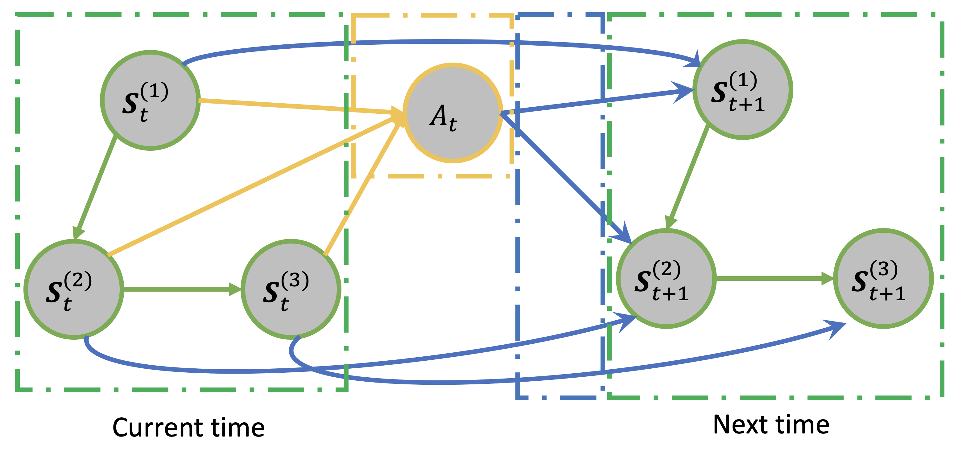
Figure 2: Example causal graph between the state and action. $\mathbf{S}_{t}^{(i)}$ is the $i$-th dimension of the interested state $\mathbf{S}$ at time $t$. Each vertex also has a corresponding exogenous variable, which has no parent and its only child is the associated endogenous variable. Per causality conventions, the exogenous variables are omitted in the graph.

First, we notice that there are three types of causal relations between the states and actions: intra-state, policy-defined, and transition-defined relations. As shown in Fig. 2, the green directed edges represent the intra-state relations, which are defined by the underlying causal mechanism. The orange edges describe the policy and represent how the state variables affect the action. The third type of relation shown as blue edges is the causal relationship between the states across different times. They represent the dynamics of the environment and depend on the transition probability $P(\mathbf{s}_{t},a_{t},\mathbf{s}_{t+1})$ in the MDP.

We assume that the intra-state and transition-defined causal relations are captured by the causal graph skeleton. For the policy-defined relations, we assume a general case where all state features are the causal parents of the action. In the causal graph, each edge defines a causal relation, and the vertex defines a variable $V$ with a causal structural function $f$. Then we only need to learn the causal structural functions between the vertices. To achieve this, we can learn each vertex’s function separately. For a vertex $V_{i}$ and its parents $\mathcal{P}a_{i}$, based on Eq. (1), we make an additive noise assumption to simplify the problem and formulate the function mapping between $V_{i}$ and $\mathcal{P}a_{i}$ as

$$V_{i}=f_{i}(\mathcal{P}a_{i})+U_{i},$$ (2)

where $U_{i}$ is an exogenous variable. We note that the additive noise assumption is widely used in the causal discovery literature (Hoyer et al. 2008; Peters et al. 2014). We then use supervised learning to learn the function mapping among the vertices. Specifically, $f_{a}$ for action $a_{t}$ is defined as

$$A_{t}=f_{a}(\mathbf{S}_{t}^{(1)},\cdots,\mathbf{S}_{t}^{(m)},U_{a}),$$

where $m$ is the dimension of the state, and $U_{a}$ is the exogenous variable for the actions.

For the state variables, we denote all exogenous variables as a vector $\mathbf{U_{S}}:=[U_{1},\cdots,U_{m}]$ and learn the structural functions. Intuitively, the exogenous variables $U_{a}$ and $\mathbf{U_{S}}$ represent not only random noise but also hidden features or the stochasticity of the policy for the intra-state and policy-defined causal relations. For transition-defined relations, the exogenous variables can be regarded as the stochasticity in the environment.

5.2 Action-based Importance

Given a state $\mathbf{s}_{t}$ and an action $a_{t}$, the importance vector $\mathbf{w}_{t}$ is calculated by applying intervention on the learned SCM. Based on the additive noise assumption, we recover the values of the exogenous variables $\mathbf{U_{s}}$ and $U_{a}$ according to the value of $a_{t}$, $\mathbf{s_{t}}$ and the learned causal structural functions. Then we define $\mathbf{w}_{t}$ using the intervention operation (counterfactual reasoning). Specifically, we define the importance vector $\mathbf{w}_{t}=[\mathbf{w}_{t}^{(1)},\cdots,\mathbf{w}_{t}^{(m)}]$ as

$$\mathbf{w}_{t}^{(i)}=\frac{\left|\left(\left.A_{t,\mathbf{S}_{t}^{(i)}=\mathbf{s}_{t}^{(i)}+\delta}\right|\mathbf{S}_{t}=\mathbf{s}_{t},A_{t}=a_{t}\right)-a_{t}\right|}{\delta},$$ (3)

where $|\cdot|$ is a vector norm (e.g., absolute-value norm) and $\delta$ is a small perturbation value chosen according to the problem setting. The term $A_{t,\mathbf{S}_{t}^{(i)}=\mathbf{s}_{t}^{(i)}+\delta}|\mathbf{S}_{t}=\mathbf{s}_{t},A_{t}=a_{t}$ represents the counterfactual outcome of $A_{t}$ if we set $\mathbf{S}_{t}^{(i)}=\mathbf{s}_{t}^{(i)}+\delta$. In our case, the value of the exogenous variables can be recovered using the additive noise assumption, so the value of $A_{t,\mathbf{S}_{t}^{(i)}=\mathbf{s}_{t}^{(i)}+\delta}|\mathbf{S}_{t}=\mathbf{s}_{t},A_{t}=a_{t}$ can be determined. We interpret the result as that the features with a larger $\mathbf{w}_{t}^{(i)}$ have a more significant causal impact on the agent’s action $a_{t}$. Note that in the simulation, we average the importance from both positive and negative $\delta$ and return the average as the final score. The perturbation amount $\delta$ is a hyperparameter and should be selected according to each problem setting.

5.3 Q-value-based Importance

While action-based importance can capture the causal impact of states on the change of the action, it may not capture the more subtle causal importance when the selected action does not change, especially when the action space is discrete. Specifically, $A_{t,\mathbf{S}_{t}^{(i)}=\mathbf{s}_{t}^{(i)}+\delta}|\mathbf{S}_{t}=\mathbf{s}_{t},A_{t}=a_{t}$ may not change after a perturbation of $\delta$, which will result in a $\mathbf{w}_{t}^{(i)}=0$. However, this is different from when there are no causal paths from feature $\mathbf{S}_{t}^{(i)}$ to the action $A_{t}$, also resulting in a $\mathbf{w}_{t}^{(i)}=0$. Therefore, we also define Q-value-based importance as follows:

$${{}^{Q}}\mathbf{w}_{t}^{(i)}=\frac{|Q_{\pi}^{\text{perturb}}-Q_{\pi}(\mathbf{s}_{t},a_{t})|}{\delta},$$ (4)

where $Q_{\pi}^{\text{perturb}}=Q_{\pi}(\mathbf{S}_{t,\mathbf{S}_{t}^{(i)}=\mathbf{s}_{t}^{(i)}+\delta},A_{t,\mathbf{S}_{t}^{(i)}=\mathbf{s}_{t}^{(i)}+\delta}|\mathbf{S}_{t}\!=\!\mathbf{s}_{t},A_{t}\!=\!a_{t})$. In detail, we use counterfactual reasoning to compute the counterfactual outcome of $A_{t}$ and $S_{t}$ after setting $\mathbf{S}_{t}^{(i)}=\mathbf{s}_{t}^{(i)}+\delta$ and then substituting them into $Q_{\pi}$ to evaluate the corresponding Q-value. Similar to the action-based importance, we account for both positive and negative importance in practice. See the Blackjack Section 6.3 in evaluation for a comparison between Eq. (3) and Eq. (4) on an example with a discrete action space.

In most RL algorithms, Q-value critically impacts which actions to choose. Therefore, we consider Q-valued-based importance as explanations on the action through the Q-value. However, we note that the Q-value-based importance method sometimes cannot reflect which features the policy really depends on. Some features may contribute largely to the Q-value of all state-action pairs ({$Q(\mathbf{s}_{t},a_{t}),a_{t}\in\mathcal{A}\}$, but not to the decision making process - the action with the largest Q-value ($\arg\max_{a_{t}\in\mathcal{A}}Q(\mathbf{s}_{t},a_{t})$). In such cases, these features may have an equal impact on the Q-value regardless of the action. For example, in the crop irrigation problem, crop pests have an impact on the crop yield (Q-value) but don’t impact the amount of irrigation water (the action). Some related simulations are shown in Appendix C. In summary, we suggest using the action-based importance method by default and the Q-value-based method as a supplement.

5.4 Temporal Importance and Cascading SCM

Temporal importance allows us to quantify the impact of past states and actions on the current action. In RL, estimating of temporal effect is important because policies are generally non-myopic, and actions should affect all future states and actions. To measure the importance beyond the previous step, we define an extended causal model that includes state features and actions in the previous time step, as shown in Fig. 1. In this model, the vertices in the graph are $\{\mathbf{S}_{\tau},A_{\tau}\}_{\tau=1}^{T}$. For simplicity, we assume the system is stationary, so the causal relations are stationary and do not change over time. Therefore, the structural functions are the same as those defined in Fig. 2, i.e., the mechanism of an edge $(\mathbf{S}_{\tau}^{(i)},\mathbf{S}_{\tau+1}^{(j)})$ will be the same as the edge $(\mathbf{S}_{t}^{(i)},\mathbf{S}_{t+1}^{(j)})$. The extended causal model can be regarded as a cascade of multiple copies of the same module, where each module is similar to that in Fig. 2. We can estimate the effect of perturbing any features or actions at any step through intervention, and the effect will propagate through the modules to the final time step. We illustrate the temporal importance in the Blackjack experiment in Section 6.3.

5.5 Comparison with Associational Methods

In Eq. (3), we define importance by applying intervention. If we change the $do$ action to the conditioning operation, we have the following definition, which is the same as the association-based saliency map method:

$${{}_{\text{sal}}}\mathbf{w}_{t}^{(i)}\!=\!\frac{\left.|A_{t}|\mathbf{S}_{t}\!=\![\mathbf{s}_{t}^{(1)},\cdots\!,\mathbf{s}_{t}^{(i)}\!+\!\delta,\cdots\!,\mathbf{s}_{t}^{(m)}]-a_{t}\right|}{\delta}$$ (5)

Associational models cannot perform individual-level counterfactual reasoning and hence cannot infer the counterfactual outcome after changing the value of one feature of the current state. As pointed out by (Pearl 2009), counterfactual reasoning can infer the specific property of the considered individual that is related to the exogenous variables, and then derives what would have happened if the agent had been in an alternative state. In our method, we use counterfactual reasoning to recover the environment at the current state and estimate how the action responds to the change in one of the state features. So our causal importance can capture more insights compared to the associational methods.

In Fig. 3, we use a one-step MDP toy example to demonstrate the difference. Omitting the time step subscript in the notation, we assume the policy is defined on the state space $\mathbf{S}=[\mathbf{S}^{(1)},\mathbf{S}^{(2)},\mathbf{S}^{(3)}]$. An observed variable $V_{p}$ is a causal parent of $\mathbf{S}^{(3)}$ but is not defined in the state space. We define the ground truth of the state and policy as Eq. (6), where $c_{1},c_{2},c_{3},c_{12},c_{p}$ are constant parameters and $U_{a},U_{1},U_{2},U_{3},U_{p}$ are exogenous variables. We use a linear SCM to show the difference between the two methods. We do not assume the SCM to have linear dependencies.

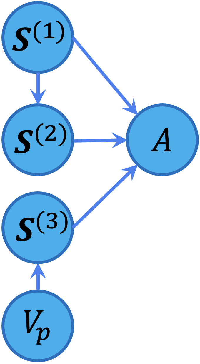
$$\begin{cases}\mathbf{S}^{(1)}&=\!U_{1}\\ \mathbf{S}^{(2)}&=\!c_{12}\mathbf{S}^{(1)}\!+\!U_{2}\\ \mathbf{S}^{(3)}&=\!c_{p}V_{p}\!+\!U_{3}\\ A&=\!c_{1}\mathbf{S}^{(1)}\!+\!c_{2}(\mathbf{S}^{(2)})^{2}\!+\!c_{3}\mathbf{S}^{(3)}\!+\!U_{a}\\ V_{p}&=\!U_{p}\end{cases}$$ (6)

Figure 3: Example of a one-step MDP

We assume that both the associational method saliency map and our causal method can learn the ground truth functions. Given a state $\mathbf{s}$, the importance vectors using the two methods are compared in Table 1. We notice that, for $\mathbf{s}^{(1)}$, our method can capture the effect of $\mathbf{s}^{(1)}$ through two causal chains $\mathbf{S}^{(1)}\!\to\!A$ and $\mathbf{S}^{(1)}\!\to\!\mathbf{S}^{(2)}\!\to\!A$, while the saliency map method captures only $\mathbf{S}^{(1)}\!\to\!A$. Our causal method considers the fact that a change in $\mathbf{S}^{(1)}$ will result in a change of $\mathbf{S}^{(2)}$ and thus additionally influence the action $A$. The non-direct paths are also meaningful in explanation and should be considered in measuring the importance of $\mathbf{S}^{(1)}$. However, they are ignored in the saliency map method. The causal importance vector for $\mathbf{s}^{(1)}$ also considers the effect of $u_{2}$, which is recovered through counterfactual reasoning. This makes the causal-based importance specific to the current state. Additionally, our method can calculate the effect of $V_{p}$ on the action $A$, which can not be achieved by the associational method saliency map.

Table 1: Importance vector on the environment in Fig. 3 using our method and the saliency map method.

	Our method	Saliency map
$\mathbf{s}^{(1)}$	$c_{1}+c_{2}c_{12}(c_{12}(2\mathbf{s}^{(1)}+\delta)+2u_{2})$	$c_{1}$
$\mathbf{s}^{(2)}$	$c_{2}(2\mathbf{s}^{(2)}+\delta)$	$c_{2}(2\mathbf{s}^{(2)}+\delta)$
$\mathbf{s}^{(3)}$	$c_{3}$	$c_{3}$
$v_{p}$	$c_{p}c_{3}$	N/A

We also note that for features $\mathbf{s}^{(2)}$ and $\mathbf{s}^{(3)}$, the two methods obtain the same result. In cases where a state feature is (1) not a causal parent of other features, (2) the policy is deterministic, and (3) there are no exogenous variables, our method is equivalent to the saliency-style approach. However, these conditions may not be common in RL. In general, there are causal relations among state features, such as the chess positions in the game of chess, the state features [position, velocity, acceleration] in a self-driving problem, and the state features [radiation, temperature, humidity] in a greenhouse control problem.

6 Evaluation

We test our causal explanation framework in three toy environments: crop irrigation (Section 6.1), collision avoidance (Section 6.2), and Blackjack (Section 6.3). We also conduct experiments on Lunar Lander, which is a more sophisticated RL environment (Appendix A.4). For each experiment, the system dynamics, policy, training details, and perturbation values used can be found in Appendix A.

6.1 Crop Irrigation Problem

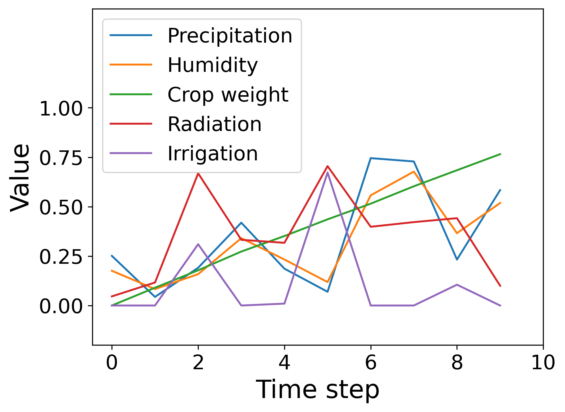
(a) A trajectory of the crop irrigation problem

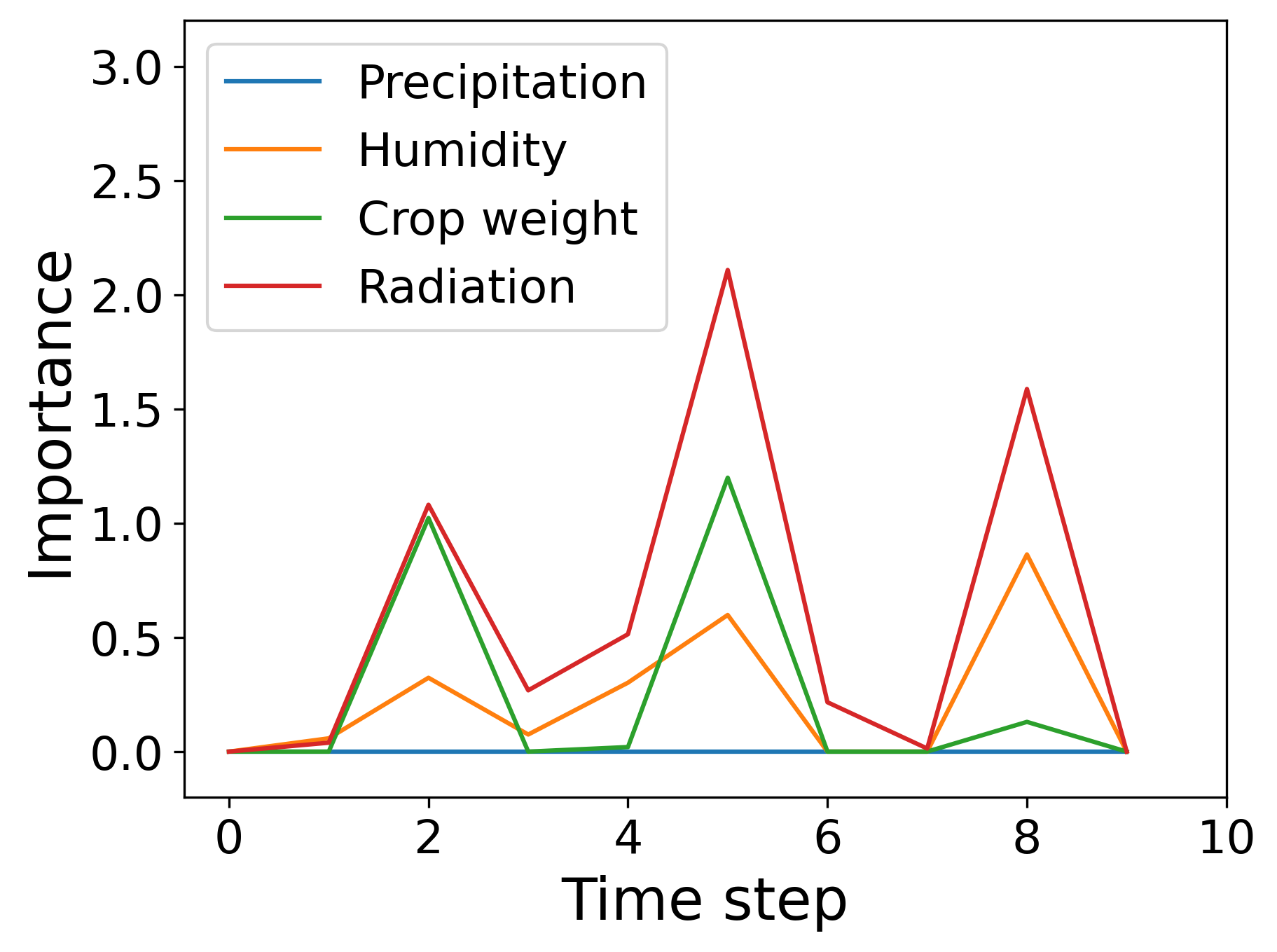
(b) Saliency map method result

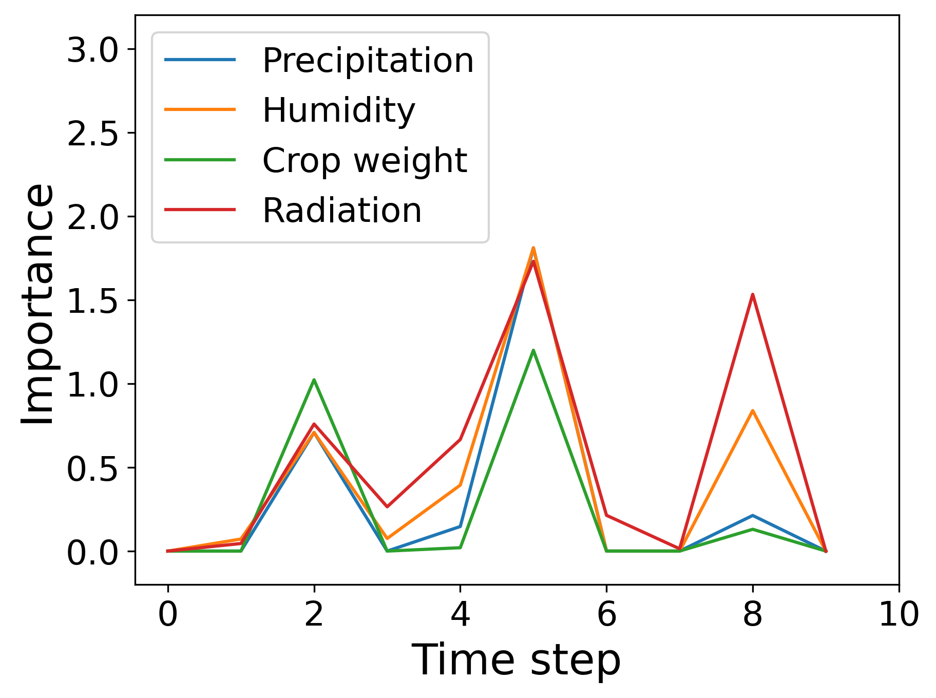
(c) Causal-based importance result

Figure 10: Importance vector for state in crop irrigation problem

We show the results of our explanation algorithm for the crop irrigation problem. We assume a simplified environment dynamic based on agriculture models (Williams et al. 1989). The growth of the plant at each step is determined by the state features humidity ($H_{t}$), crop weight ($C_{t}$), and radiation ($D_{t}$). The policy controls the amount of water to irrigate each day. Intuitively, it irrigates more when the crop weight is high, and less when the crop weight is low. Details about the environment dynamics and policy are described in Appendix A.1. We use Fig. 1 as the causal skeleton and apply a neural network to learn the structural equations. Fig. 4 shows the importance vector of the state for a given environment $[P_{t}=0.07,H_{t}=0.12,C_{t}=0.44,D_{t}=0.70]$ and its corresponding action $I_{t}=0.67$. First, we notice that our method can estimate the importance of the feature precipitation($P_{t})$, which is not defined in the state space of the policy. Second, in estimating the causal importance of $H_{t}$, our method can estimate the effect of $H_{t}\to C_{t}\to I_{t}$, which results in higher importance compared to the saliency map method. Since an intervention on $H_{t}$ can induce a change in $C_{t}$, causing the action to change more drastically. This effect cannot be measured without a causal model. The same applies to the feature $D_{t}$. The full trajectory and the importance vector at each time step can be found in Fig. 10 in Appendix A.1.

The causality-based action influence model (Madumal et al. 2020) can find a causal chain $I_{t}\to\ C_{t}\to\,$CropYield and provide the explanation as “the agent takes current action to increase $C_{t}$ at this step, which aims to increase the eventual crop yield.” This explanation only provides the information that $C_{t}$ is an important factor in the decision-making for the current action but can’t quantify it. Moreover, this explanation can’t provide information for other state features, such as $H_{t}$ and $D_{t}$ which are also measured in our importance vector.

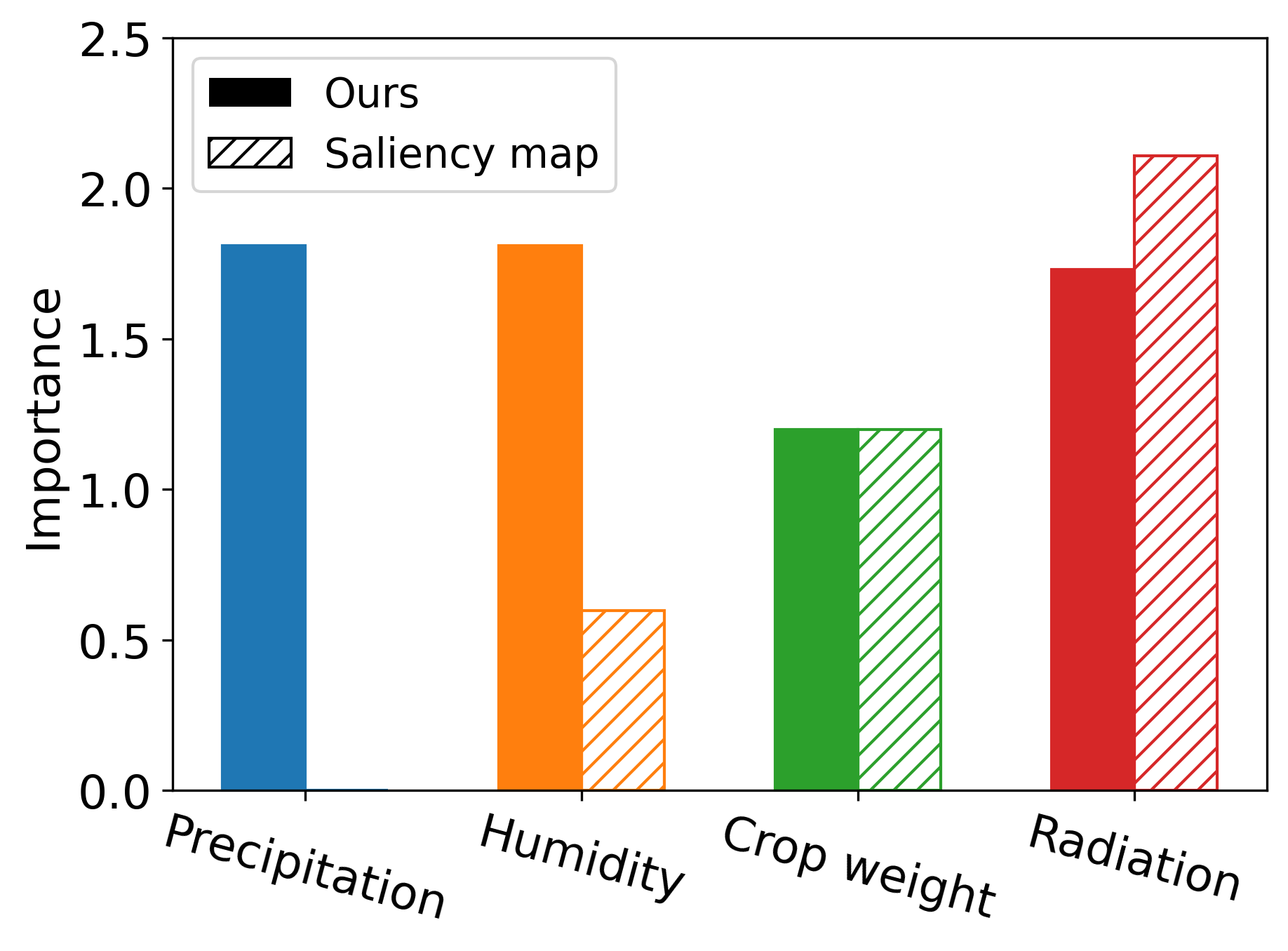
Figure 4: The importance vector for the crop irrigation problem.

6.2 Collision Avoidance Problem

We use a collision avoidance problem to further illustrate that our causal method can find a more meaningful importance vector than saliency map, i.e., which state feature is more impactful to decision-making.

Fig. 5(a) shows the state definition for this problem. A car with zero initial velocity travels from the start point to an endpoint over a distance of $X_{\textrm{goal}}$. The system is controlled in a discrete-time-slot manner and we assume acceleration of the car is constant within each time step. The state $\mathbf{S}_{t}$ includes the distance from the start $X_{t}$, the distance to the end $D_{t}$, and the velocity $V_{t}$ of the car, i.e., $\mathbf{S}_{t}:=[V_{t},X_{t},D_{t}]$, where $V_{t}\leq v_{\max}$ and $v_{\max}$ is the maximum speed of the car. The action $A_{t}$ is the car’s acceleration, which is bounded $|A_{t}|\leq e_{\max}$. We assume the acceleration of the car is constant within each time step. More detailed settings are described in the simulation section in the supplementary materials. The objective is to find a policy $\pi$ to minimize the traveling time under the condition that the final velocity is zero at the endpoint (collision avoidance).

An RL agent learns the following optimal control policy for this avoidance problem, which is also known as the bang-bang control (optimal under certain technical conditions) (Bryson 1975):

$$A_{t}=\begin{cases}e_{\max}&\text{if }D_{t}\leq{v_{\max}^{2}}/({2e_{\max}})\\ -e_{\max}&\text{otherwise}\end{cases}$$ (7)

Intuitively, this policy accelerates as much as possible until reaching the critical point defined above. Then it will decelerate until reaching the goal.

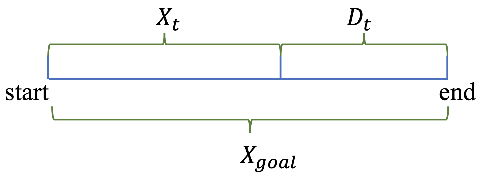
(a) The state definition

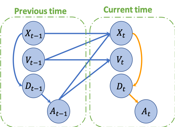
(b) The causal graph of states and actions

Figure 5: The collision avoidance problem and its corresponding SCM skeleton.

We use Fig. 5(b) as the SCM skeleton and use linear regression to learn the structural equations as the entire dynamics are linear. The detail about the system dynamics is described in the appendix.

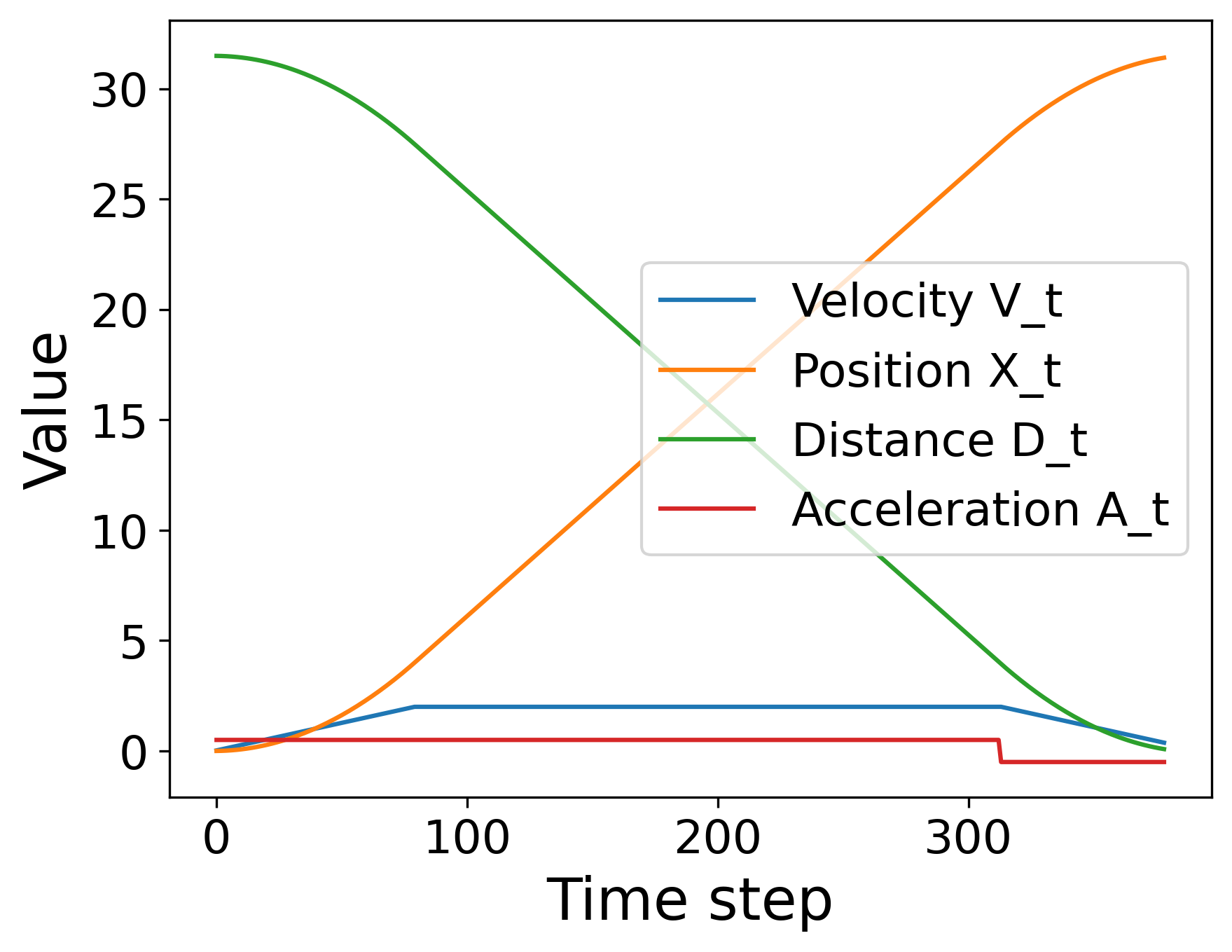
(a) A trajectory of using bang-bang control on the collision avoidance problem.

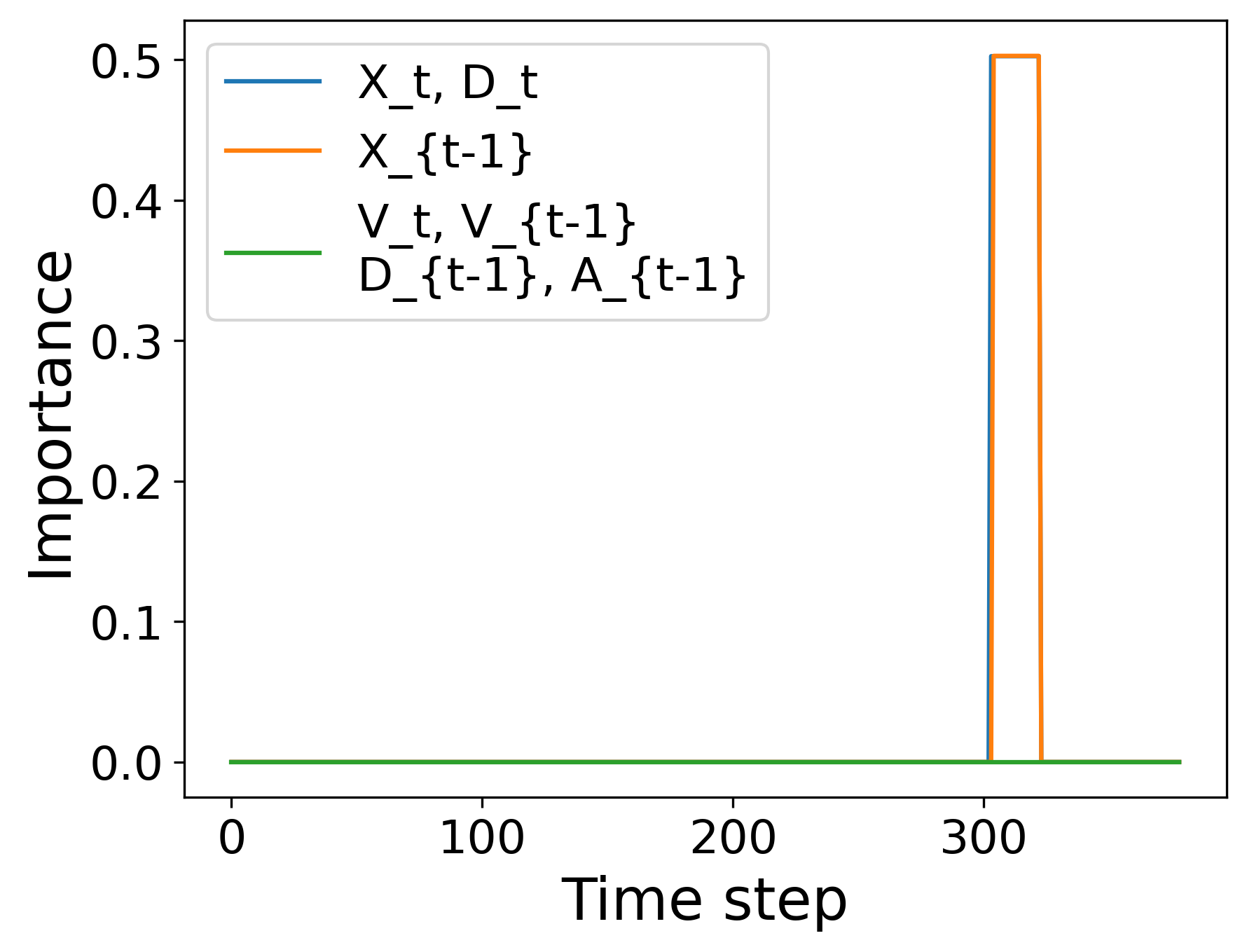
(b) The result importance from our algorithm on the trajectory in Fig. 6(a).

Figure 6: Trajectory and importance on the collision avoidance problem

Fig. 6(a) shows a trajectory under the policy bang-bang control and Fig. 6(b) shows its corresponding causal importance results. The importance of $V_{t},A_{t-1},D_{t-1},V_{t-1}$ are zero throughout the time history, and those of $X_{t},D_{t},X_{t-1}$ have peak importance of $[0.502,0.502,0.502]$ , respectively, between time step 303-322, during which the car changes the direction of acceleration to avoid hitting the obstacle. The importance curves of $X_{t}$, $D_{t}$, and $X_{t-1}$ have the same shape, but that of $X_{t-1}$ is off by one time step, corresponding to their time step subscript. If we were to use the associational saliency method (Greydanus et al. 2018) $X_{t}$ would have a constant zero importance since the action is solely determined by the feature $D_{t}$. In comparison, our method can find non-zero importance through the edge $X_{t}\to D_{t}$. It is reasonable that $X_{t}$ causally affects $A_{t}$, because, in the physical world, the path length $X_{t}$ is the cause of the measurement of the distance to the end $D_{t}$. Although in Eq. (7) the action $A_{t}$ is only decided by $D_{t}$, the source cause of the change in $D_{t}$ is $X_{t}$. We can only obtain such information through a causal model, not an associational one.

6.3 Blackjack

We test our explanation mechanism on a simplified game of Blackjack. The state is defined as [hand, ace, dealer], where hand represents the sum of current cards in hand, ace represents if the player has a usable ace (an ace that can either be a 1 or an 11), and dealer, is the value of the dealer’s shown card. There are two possible actions: to draw a new card or to stick and end the game. We use an on-policy Monte-Carlo control (Sutton and Barto 2018) agent to test our mechanism. Since the problem dynamic is non-linear, we use a neural network to learn each structural equation. Fig. 7 shows the skeleton of the SCM. More details about the rules of the game are explained in Appendix A.2. Note that in Blackjack, the exogenous variable $U_{i}$ of some features can be interpreted as the stochasticity or the “luck” during the input trajectory. e.g., $U_{\texttt{hand},t}$ corresponds to the value of the card drawn at step $t$ if the previous action is draw.

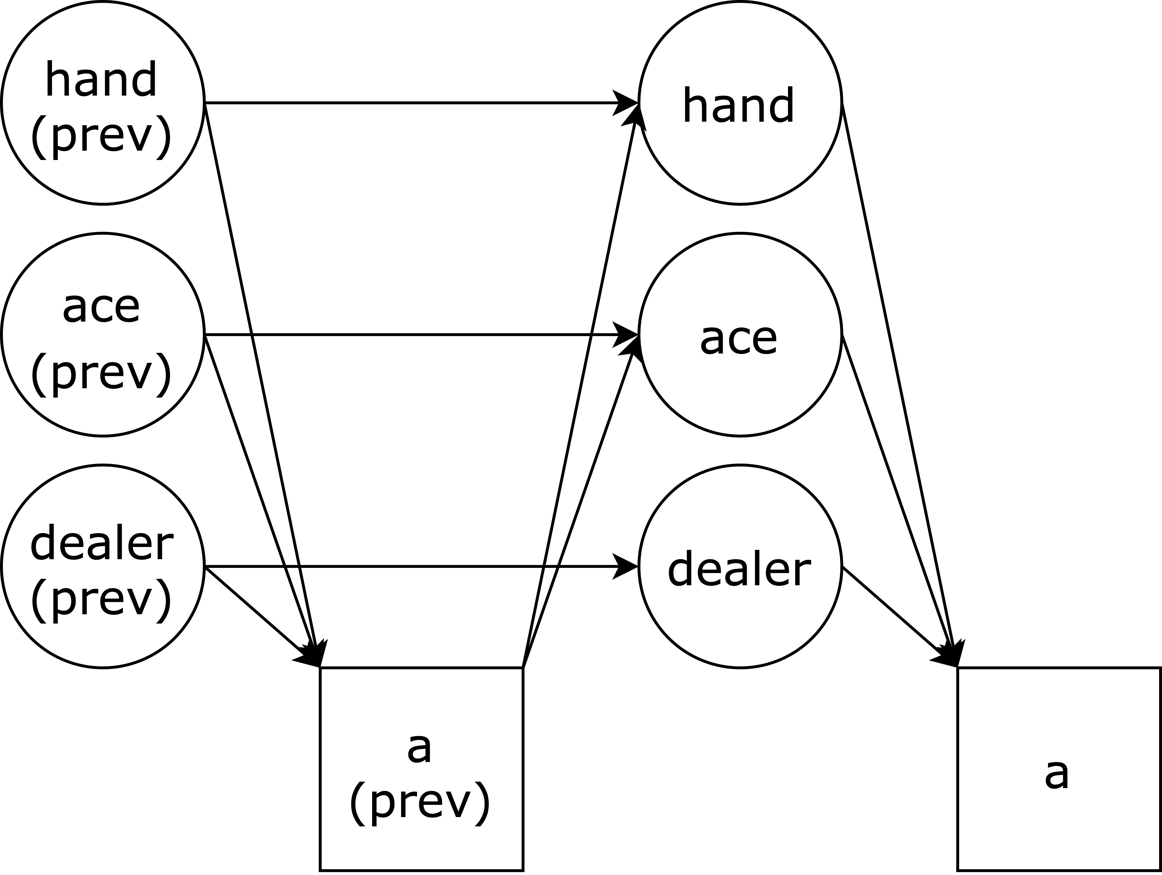
Figure 7: The skeleton of the Blackjack SCM.

Using Q-values as Metric

The solid bars in Fig. 8 on the next page show the result of Q-value-based importance based on Eq. (4). We interpret the result as follows: (1) The importance of all features are highest at step 1. This is because state 1 is closest to the decision boundary of the policy, and thus applying a perturbation at this step is easier to change the Q-value distribution; (2) The importance of dealer and dealer_prev are the same throughout the trajectory. This is due to the fact that dealer and dealer_prev are always the same. Thus, applying a perturbation on dealer_prev will have the same effect as applying a perturbation on dealer assuming changing dealer_prev won’t incur a change in the previous action; (3) A similar phenomenon can be observed between hand and hand_prev. Increasing the hand at step $t-1$ by one will have the same outcome as drawing a card with one higher value at $t$. The occasional difference comes from the change in hand_prev causing a_prev to change; (4) The importance of ace is highest at steps 2 and 5. In both of these two states, changing if the player has an ace or not while keeping other features the same will change the best action and a larger difference in the Q-values, which causes the importance to be higher.

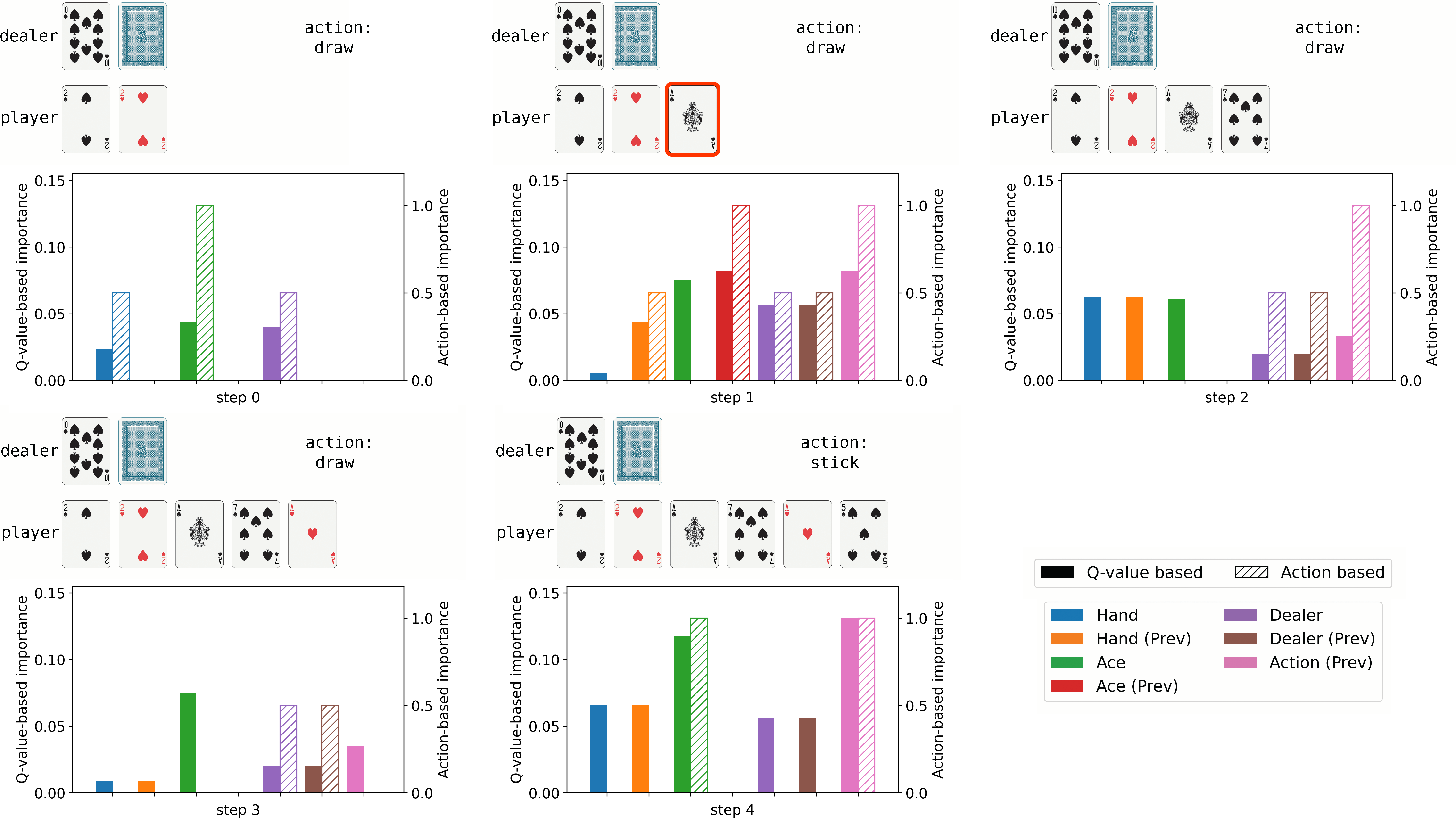
Figure 8: A trajectory of a blackjack game and the result from running our mechanism using either the Q-values or the action as the metric. In each sub-graph, the top figure shows the state, and the usable ace is highlighted in red if present. The bottom figure shows the importance of each feature. The solid bars are the Q-value-based importance and the hatched bars are the action-based importance. Note that at step 1, the importance for the previous hand, previous dealer, previous ace, and previous action are not applicable since there is no previous state for the first state.

Using Action as Metric

The hatched bars in Fig. 8 show the result of action-based importance based on Eq. (3). The importance is more “bursty”, and features, such as hand, have an importance of zero in the majority of the steps since a perturbation of size one could not trigger a change in the action. However, intuitively, hand is crucial to the agent’s decision-making. Therefore, in this case, we note that the Q-value-based method produces a more reasonable explanation in this example.

Multi-Step Temporal Importance

We cascade the causal graph of blackjack in Fig. 7 to estimate the impact of the past states and actions on the current action, and the full SCM is shown in Fig. 12 in Appendix A.2. Fig. 9 shows the results of Q-value-based importance. The importance of $A_{4}$ on itself is omitted since it will always be one regardless of any other part of the graph. We interpret the results as follows: (1) The importance of hand_τ and dealer_τ is flat over time. As discussed above, perturbing these two features at any given step will mostly change the last state in the same way, resulting in constant importance; (2) The importance of the action $a_{\tau}$ increases as $\tau$ gets closer to the last step $t=4$. An action taken far in the past should generally have a smaller impact on the current action, which corresponds to the increasing importance for a_τ in our explanation.

6.4 Additional Evaluation

We also evaluate our scheme in a more complex RL environment, Lunar Lander, in Appendix A.4. Lunar Lander is a simulation testing environment developed by OpenAI Gym (Brockman et al. 2016). The simulation shows that our scheme can explain some specific phases(state) of the spaceship in the landing process.

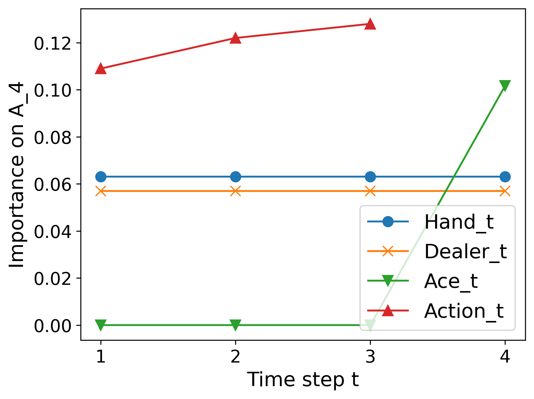
Figure 9: The Q-value-based temporal importance on $A_{4}$ for all state features and actions at past time steps in the Blackjack experiment.

7 Discussions

Our causal importance explanation mechanism is a post-hoc explanation method that uses data collected by an already learned policy. We focus on providing local explanations based on a particular state and action. Counterfactual reasoning is required to recover the exogenous variables and estimate the effect on the given state and action. In this case, the intervention operation is not enough to achieve this goal, as it can only evaluate the average results (population) over the exogenous variables, which is not a local explanation for the given state.

Intra-state Relations

One crucial characteristic of our method is that we consider intra-state relations when computing the importance, which is essential in accurately quantifying the impact of a state feature on the action. Although the MDP defines that a state feature at a certain time step cannot affect another state feature at the same step, it is essential to consider causal relationships within state features when measuring their impact if we use causal intervention or associational perturbation. Since these types of methods require modifying the value of a specific state feature, it should subsequently affect the value of other state features based on real-world causality. For instance, in the collision avoidance problem (Section 6.2), the distance to the end ($D_{t}$) will change in response to the distance from the start ($X_{t}$), and in the crop irrigation problem (Section 6.1), the crop weight ($C_{t}$) will vary based on the humidity level ($H_{t}$). Ignoring the intra-state causality can lead to an invalid state after the intervention, resulting in inaccurate importance estimates for the given state feature. Hence, we formulate the intra-state relations in the SCM to provide more accurate and comprehensive explanations of the problem.

Additive Noise Assumption

With the additive noise assumption in Eq. (2), the exogenous variable (noise) can be fully recovered and used for counterfactual reasoning. We note that the full recovery noise assumption can be relaxed for our mechanism. In the case where the exogenous variables have multiple values (not deterministic), we can generalize our definition of importance vector in Eq. (3) by replacing the first term with the expectation over different values of exogenous variables using probabilistic counterfactual reasoning (Glymour, Pearl, and Jewell 2016). Furthermore, the additive noise assumption is not mandatory. We can use bidirectional conditional GAN (Jaiswal et al. 2018) to model the structure function and use its noise to conduct counterfactual reasoning and obtain the importance vector.

Known SCM Skeleton Assumption

Our approach is based on the assumption that the SCM skeleton is known, which can be obtained either through background knowledge of the problem or learned using causal discovery algorithms. Causal discovery aims to identify causal relations by analyzing the statistical properties of purely observational data. There are several causal discovery algorithms available, including the classical constraint-based PC algorithm  (Spirtes et al. 2000), algorithms based on linear non-Gaussian models  (Shimizu et al. 2006), and algorithms that use the additive noise assumption  (Hoyer et al. 2008; Peters et al. 2014). These algorithms can be used to learn the SCM skeleton from observational data, which can then be used in our method to quantify the impact of state features and actions on the outcome. There are also existing toolboxes such as (Kalainathan and Goudet 2019) and (Zhang et al. 2021) that can be easily applied directly to data to identify the SCM structure.

Perturbation

In addition to the method we employed in the simulation, which averages the importance derived from both positive and negative $\delta$, maximizing them is also a viable option.To compute the causal importance vector defined in Eq. (3), we need to choose a perturbation value $\delta$. As shown in Table 1, the importance may depend on $\delta$. Therefore, it is not meaningful to compare importance vectors calculated with different $\delta$. This is a common issue of perturbation-based algorithms, including the saliency map method. In our case, $\delta$ should be as small as possible but still be computationally feasible. More detailed sensitivity analysis and normalization on the perturbation value $\delta$ can be found in Appendix B.

Limitations

Our study has limitations when the state space has high dimensions, for example, in visual RL, where state features are represented as images. Image data is inherently high-dimensional, with multiple features that can interact in complex ways. The SCMs we used may struggle to fully capture the complexity of these interactions, especially when a large number of variables are involved. To address this issue, we suggest utilizing the algorithm of causal discovery in images (Lopez-Paz et al. 2017) and representation learning (Yang et al. 2021). Further work is needed to explore this direction.

Another question that might be raised is what will happen if the trained SCM is not perfect. An imperfect SCM will cause the counterfactual reasoning result to be biased, and thus affecting the final importance. One potential solution is quantifying the uncertainty of the explanation. If the explainer can output its confidence on top of the importance score, users can identify potential out-of-distribution samples where our explanation framework might fail. To achieve this, we need to separate aleatoric uncertainty (which comes from the inherent variability in the environment) and epistemic uncertainty (which represents the imperfection of the model) (Gawlikowski et al. 2021). Our use of SCM may help us to differentiate the two, and this is one of the directions we are currently exploring.

8 Conclusion

In this paper, we have developed a causal explanation mechanism that quantifies the causal importance of states on actions and their temporal importance. Our quantitative and qualitative comparisons show that our explanation can capture important factors that affect actions and their temporal importance. This is the first step towards causally explaining RL policies. In future work, it will be necessary to explore different mechanisms to quantify causal importance, relax existing assumptions, build benchmarks, develop human evaluations, and use the explanation to improve evaluation and RL policy training.

Appendix A Additional Experiments and Details

In this section, we provide additional details regarding the crop irrigation problem, the collision avoidance problem, and the Blackjack experiments. Furthermore, we describe our results on an additional testing environment, Lunar Lander.

All experiments were conducted on a machine with 8 NVIDIA RTX A5000 GPU, an dual AMD EPYC 7662 CPU, and 256 GB RAM.

A.1 Crop Irrigation

This section contains details of the crop irrigation experiment.

System dynamics

Precipitation $$=U(0,1)$$

SolarRadiation $$=U(0,1)$$

Humidity $$=0.3\cdot\textrm{Humidity}_{\textrm{prev}}+0.7\cdot\textrm{Precipitation}$$

CropWeight $$=\textrm{CropWeight}_{\textrm{prev}}$$

$$+0.07\cdot\big{(}1-(0.4\cdot\textrm{Humidity}+0.6\cdot\textrm{Irrigation}-\textrm{Radiation}^{2})^{2}\big{)}$$

$$+0.03\cdot U(0,1)$$

The change in CropWeight at each step is determined by humidity, irrigation and radiation, and maximum growth is achieved when $0.4\cdot\textrm{Humidity}+0.6\cdot\textrm{Irrigation}=\textrm{Radiation}^{2}$. An additional exogenous variable is also included in the change of CropWeight. This can be regarded as some unobserved confounders that affect the growth that are not included in the system dynamics, such as CO₂Concentration or the temperature.

Policy

$$\textrm{Irrigation}=(\textrm{Radiation}^{2}-0.4\cdot\textrm{Humidity})\cdot(1.6\cdot\textrm{CropWeight}+0.2)/0.6$$

The policy we used is a suboptimal policy that multiplies an additional coefficient $1.6\cdot\textrm{CropWeight}+0.2$ on the optimal policy. This will cause the irrigation value to be less than optimal when CropWeight is less than 0.5, and more than optimal and vice versa.

Training

We use a neural network to learn the causal functions in the SCM. The network has three fully-connected layers, each with a hidden size of four. We use Adam with a learning rate of $3\times 10^{-5}$ as the optimizer. The training dataset consists of 1000 trajectories (10000 samples) and the network is trained for 50 epochs.

Perturbation

The perturbation value $\delta$ used in the intervention is $0.1$ w.r.t. the range of each value.

A.2 Blackjack

This section contains details and additional figures for the blackjack simulation.

System dynamics

This simulation is done in the blackjack environment in OpenAI Gym (Brockman et al. 2016). The goal is to draw cards such that the sum is close to 21 but never exceeds it. Jack, queen and king have a value of 10, and an ace can be either a 1 or an 11, and an ace is called “usable” when it can be used at an 11 without exceeding 21. We assume the deck is infinite, or equivalently each card is drawn with replacement.

In each game, the dealer starts with a shown card and a face-down card, while the player starts with two shown cards. The game ends if the player’s hand exceeds 21, at which the player loses, or if the player chooses to stick, the dealer will reveal the face-down card and draw cards until his sum is 17 or higher. The player wins if the player’s sum is closer to 21 or the dealer goes bust.

Policy

We trained the agent using on-policy Monte-Carlo control. Fig. 11 shows the policy and the decision boundary.

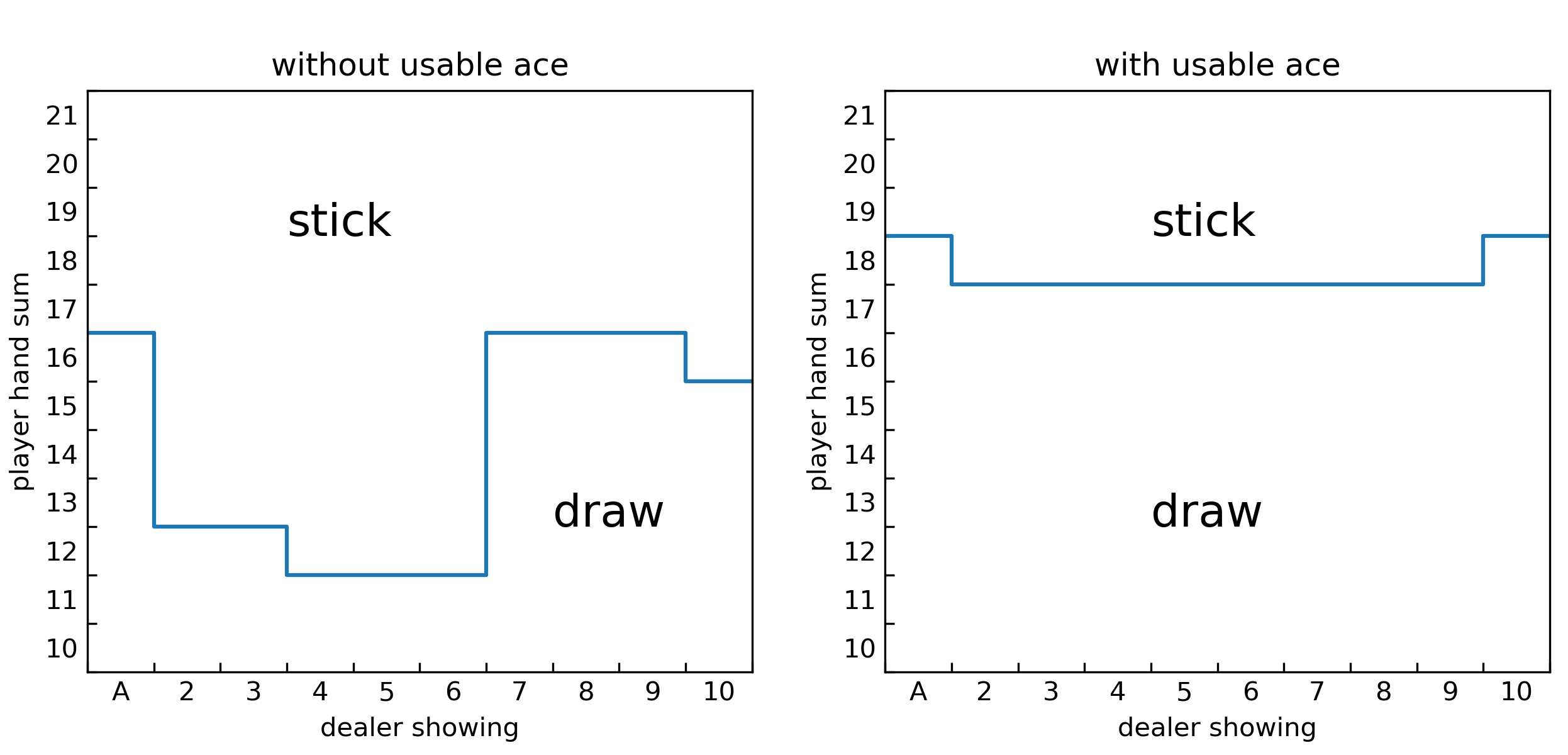
Figure 11: The policy we use for the blackjack game. The blue line shows the decision boundary.

SCM structure

We assume the blackjack game has a causal structure as shown in Fig. 7. Additionally, Fig. 12 shows the 5-step cascading SCM we used to test the temporal importance.

Figure 12: The skeleton of the cascading SCM for a 5-step blackjack game.

Training

We use a neural network to learn the causal functions in the SCM. The network has three fully-connected layers and each layer has a hidden size of four. We use Adam with a learning rate of $3\times 10^{-5}$ as the optimizer. The training dataset consists of 50000 trajectories ($\sim$76000 samples) and the network is trained for 50 epochs.

Perturbation

Since blackjack has a discrete state space, for numerical features “hand” and “dealer”, we use a perturbation value $\delta=1$. For the boolean feature “ace”, we flip its value as the perturbation.

A.3 Collision Avoidance Problem

We use the collision avoidance problem to further illustrate that our causal method can find a more meaningful importance vector than saliency map, i.e., which state feature is more impactful to decision-making.

System dynamics

The state $\mathbf{S}_{t}$ includes the distance from the start $X_{t}$, the distance to the end $D_{t}$, and the velocity $V_{t}$ of the car, i.e., $\mathbf{S}_{t}:=[V_{t},X_{t},D_{t}]$, where $V_{t}\leq v_{\max}$ and $v_{\max}$ is the maximum speed of the car. The action $A_{t}$ is the car’s acceleration, which is bounded $|A_{t}|\leq e_{\max}$. The state transition is defined as follows:

$$V_{t+1} :=V_{t}+A_{t}\Delta t$$

$$X_{t+1} :=X_{t}+V_{t}\Delta t+\frac{1}{2}A_{t}\Delta t^{2}$$

$$D_{t+1} :=X_{\text{goal}}-X_{t+1}$$

The objective of the RL problem is to find a policy $\pi$ to minimize the traveling time under the condition that the final velocity is zero at the endpoint (collision avoidance).

Policy

An RL agent learns the following optimal control policy also known as the bang-bang control (optimal under certain technical conditions) defined as Eq. (7)

SCM structure

We use Fig. 5(b) as the SCM skeleton and use linear regression to learn the structural equations as the entire dynamics are linear.

Perturbation

The perturbation value $\delta$ used in the intervention is $0.1$ after normalization.

A.4 Lunar Lander

System dynamics

Lunar lander problem is a simulation testing environment developed by OpenAI Gym (Brockman et al. 2016). The goal is to control a rocket to land on the pad at the center of the surface while conserving fuel. The state space is an 8-dimensional vector containing the horizontal and vertical coordinates, the horizontal and vertical speed, the angle, the angular speed, and if the left/right leg has contacted or not.

The four possible actions are to fire one of its three engines: the main, the left, or the right engine, or to do nothing.

The landing pad location is always at $(0,0)$. The rocket always starts upright at the same height and position but has a random initial acceleration. The shape of the ground is also randomly generated, but the area around the landing pad is guaranteed to be flat.

Policy

We train our RL policy using DQN (Van Hasselt, Guez, and Silver 2016).

Figure 13: The causal structure of lunar lander that includes previous state and actions. There should also be edges from each feature to the action at its time step, e.g. edges from x_pos_prev to a_prev, or from x_pos to a. These edges are not shown in this graph for simplicity.

SCM structure

We use the Fig. 13 as the skeleton of SCM. The structural functions are learned with linear regression using 100 trajectories ($\sim$25000 samples).

(a) The lunar lander instance.

(b) Causal importance vector the for the current-step features on the trajectory in Fig. 14(a).

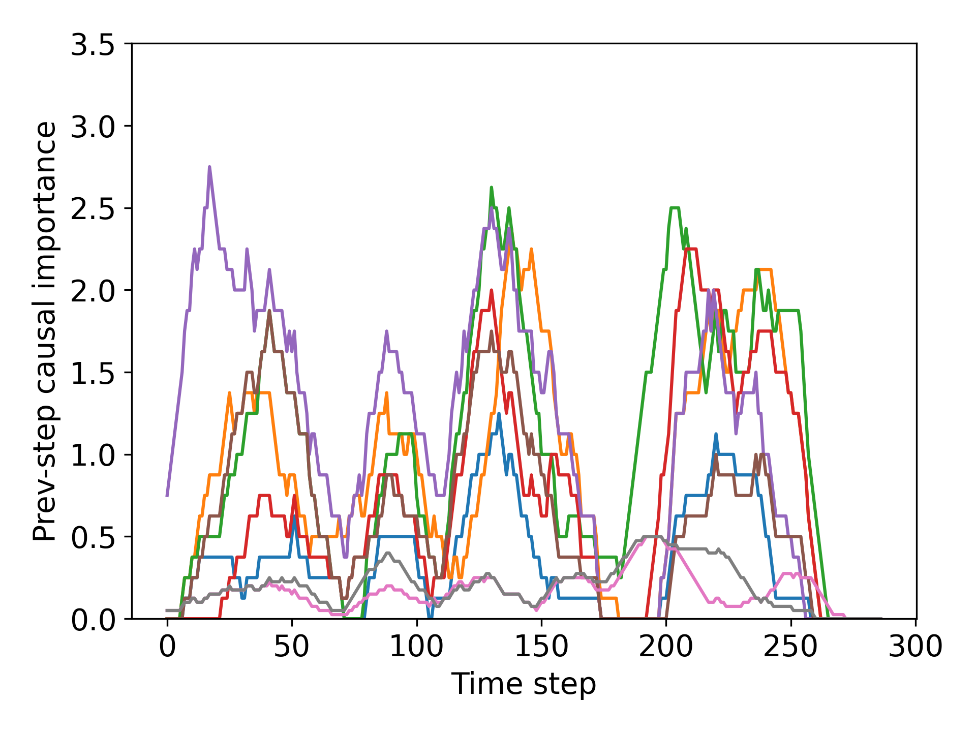
(c) Causal importance vector the for the previous-step features on the trajectory in Fig. 14(a).

Figure 14: A lunar lander trajectory instance we used to evaluate our algorithm and the corresponding causal importance vector. The “freefall phase” is roughly between steps 0-70, “adjusting phase” is between steps 70-170, and “touchdown phase” is from about step 170 to the end.

Evaluation

Fig. 14 shows a trajectory of the agent interacting with the lunar lander environment and the corresponding causal importance using our mechanism. We notice that our mechanism discovers three importance peaks, and we explain this as the agent’s decision-making during the landing process consisting of three phases: a “free fall phase”, in which the agent mainly falls straight and slightly adjusts its angle to negate the initial momentum; an “adjusting phase”, in which the agent mostly fires the main engine to reduce the Y-velocity; and a “touchdown phase”, during which the lander is touching the ground and the agent is performing final adjustments to stabilize its angle and speed. Fig. 15(a), 15(b) and 15(c) show our causal importance vector during each of the three phases. We notice that during the “free fall phase”, features such as angle, angular velocity and x-velocity are more important since the agent needs to rotate to negate the initial x-velocity. However, as the rocket approaches the ground during the “adjusting phase”, we find an increase in importance for y-velocity since a high vertical velocity is more dangerous to control when the rocket is closer to the ground. In the last “touchdown phase”, a large x-position and x-velocity importance can be observed as a change in those features is highly likely to cause the lander to fail to land inside the designated landing zone. Since the lander is already touching the ground, it will take much more effort for the agent to adjust compared to when the lander is still high in the air.

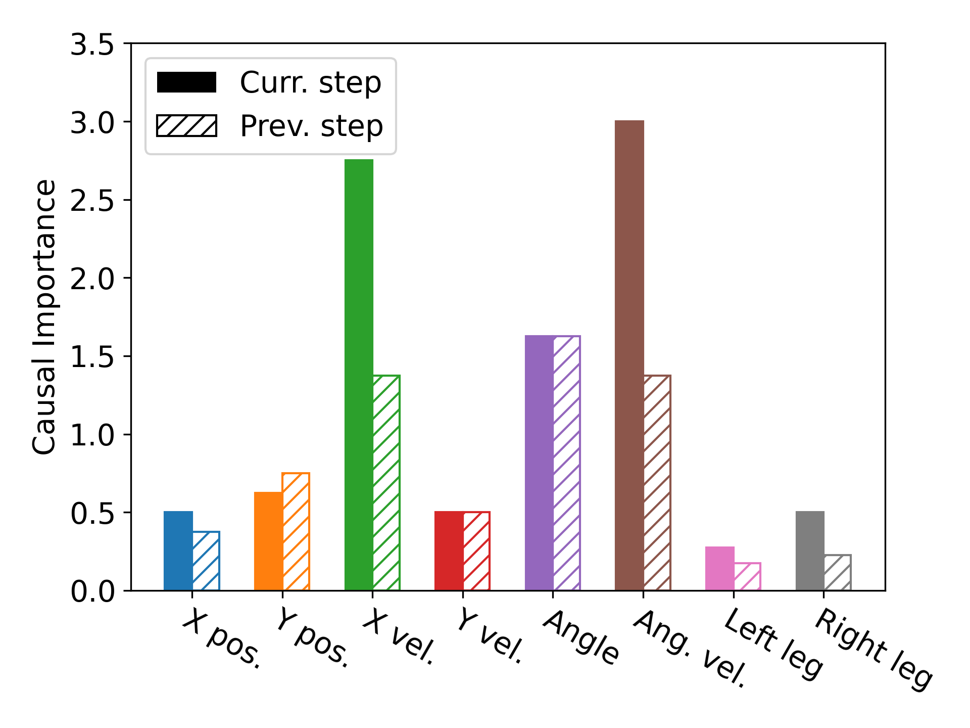
(a) Importance vector during the “free fall phase” (step 48).

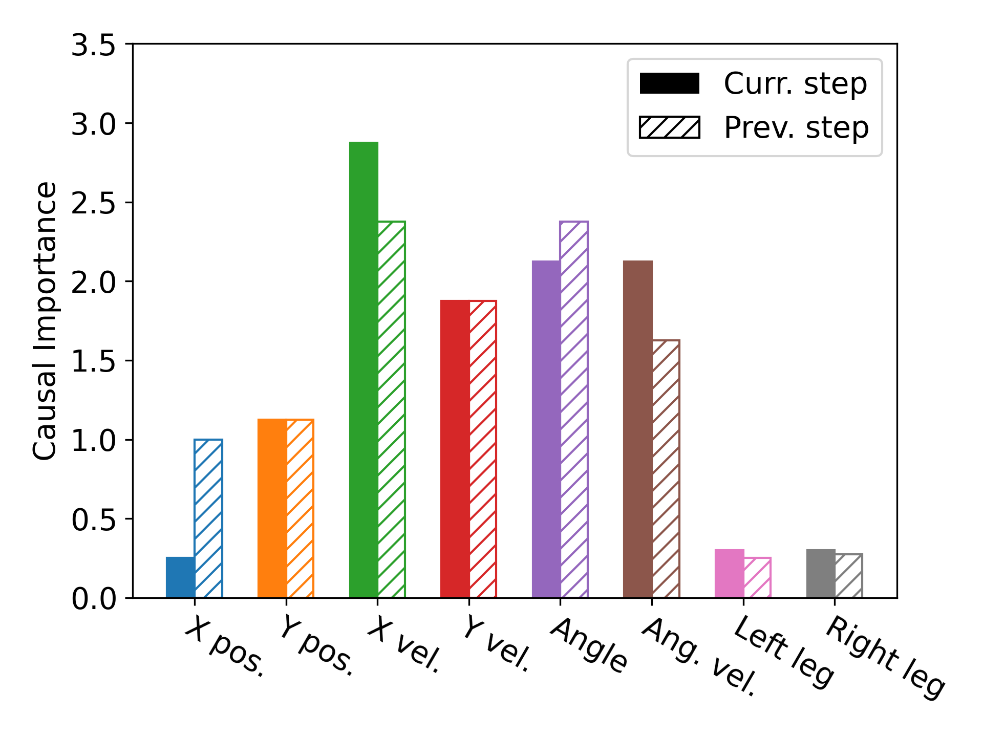
(b) Importance vector during the “adjusting phase” (step 129).

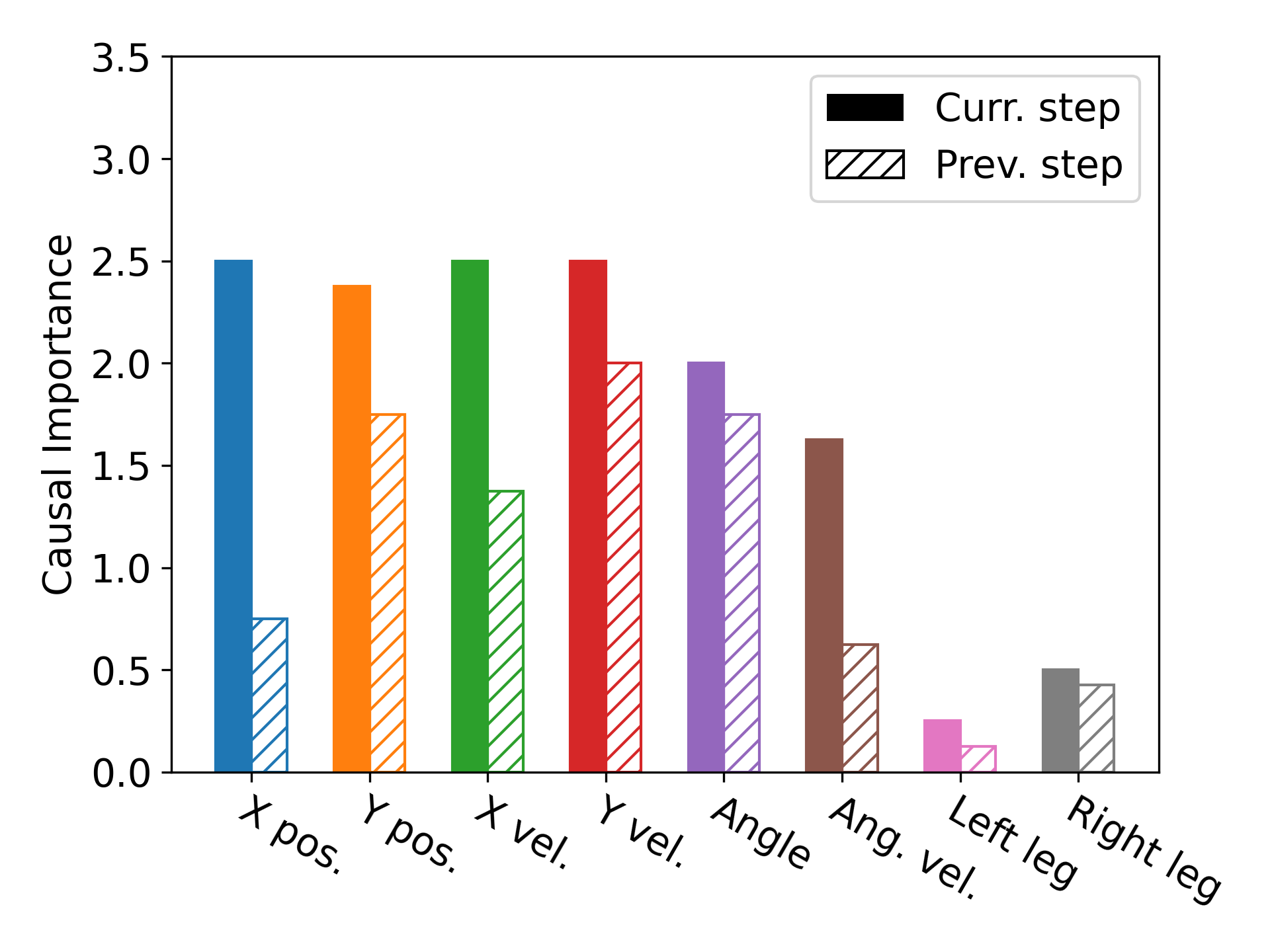
(c) Importance vector during the “touchdown phase” (step 216).

Figure 15: The importance vector on lunar lander calculated using our method and a comparison with the saliency map method. The solid bars in the first three figures representing the importance of the current-step features and the shaded bars are for the previous-step features.

The results are similar to those of saliency-based algorithms (Greydanus et al. 2018), and Fig. 16 shows the difference in importance vector between our algorithm and saliency-based algorithm. Note that differences only occur for the positions and the angle. This is because other features don’t have any additional causal paths to the action besides the direct connection. Therefore, the intervention operation is equivalent to the conditioning operation for these features. The features position and angle have an additional causal path through the legs, which causes the difference. Notably, our method captures higher importance for angle, which we interpret as that the landing angle is crucial and is actively managed by the agent.

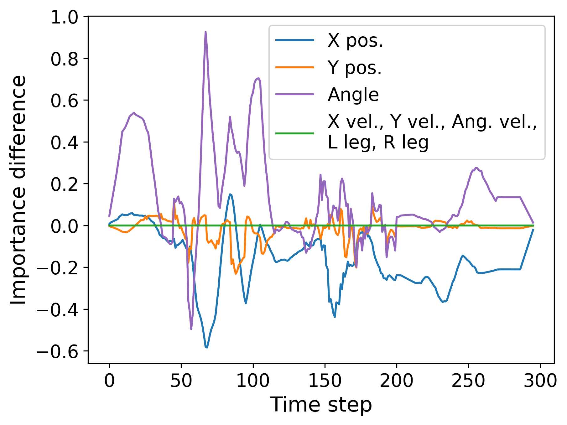
Figure 16: Difference between our method and the saliency map method for current-step features.

We are also able to compute the importance of the features in the previous steps, and Fig. 14(c) and the shaded bars in Fig. 15 represent such importance vectors. The previous-step importances are rather similar to those of the current-step features since the size of the time step is comparatively small. However, our algorithm captures that during the “adjusting phase”, the previous-step importance for the angle is in general higher than the current-step importance, as changing the previous angle may have a cascading effect on the trajectory and is especially important to the agent when it is actively adjusting the angle.

Appendix B Sensitivity Analysis

This section performs a sensitivity analysis on how the perturbation amount affects the result of our explanation.

For action-based importance, too small of a perturbation may not yield a meaningful result. This is due to the fact that, depending on the environment and the policy, a too small perturbation may fail to trigger a noticeable change in the action, resulting in a zero importance. This differs from the zero importance case where the policy disregards the feature when making decisions. In our experiments, we use 0.01 with respect to the range of the features for continuous features and the smallest unit for discrete features.

In general, using different perturbation amounts $\delta$ on the same state in the same SCM may result in different importance vectors, and vectors calculated using different $\delta$ cannot be meaningfully compared. However, if we desire the importance of using different $\delta$ to be more on the same level, we suggest finding the highest importance across all features and all time steps and normalizing all results by said number. Section B.2 contains an example comparing the importance score with and without the aforementioned normalization.

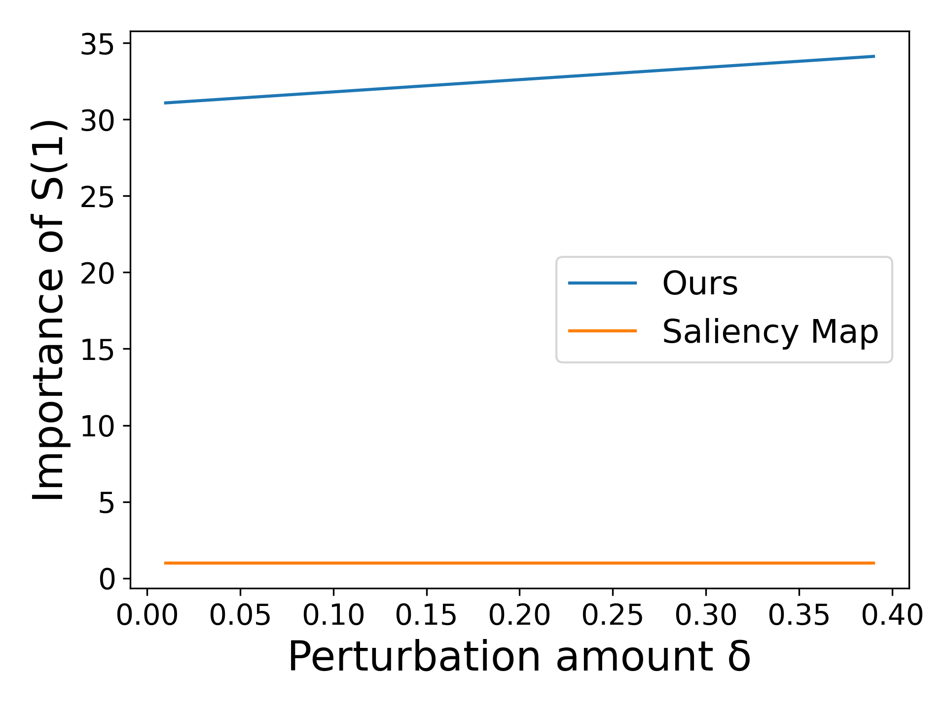
Figure 17: The importance vector of $\mathbf{S}^{(1)}$ from both our method and the saliency map method with respect to the perturbation amount.

B.1 One-step MDP

As we demonstrated in the example of one-step MDP in Fig. 3 and Table 1, our importance vector will sometimes be affected by the perturbation amount. For this experiment, we use Fig. 3 as the skeleton and the following settings. The constants are

$$c_{1}=1,c_{2}=-2,c_{3}=3,c_{12}=2,c_{p}=-1$$

We use unit Gaussian distributions as the exogenous variables and the values are

$$u_{1}=0.50,u_{2}=-0.14,u_{3}=0.65,u_{p}=1.52,u_{a}=-0.23$$

The state value and the corresponding action are then

$$\mathbf{s}^{(1)}=0.50,\mathbf{s}^{(2)}=0.86,\mathbf{s}^{(3)}=-0.88,v_{p}=1.52,a=3.83$$

The result of running our method and the saliency map method on the feature $\mathbf{S}^{(1)}$ is shown in Fig. 17. Same as in Table 1. Our algorithm is linear w.r.t. $\delta$ while the saliency map result is constant. The increased importance comes from the causal link $\mathbf{S}^{(1)}\!\to\!\mathbf{S}^{(2)}\!\to\!A$, which also introduces the linear relationship.

B.2 Collision Avoidance

Fig. 18 shows the importance vector of $X_{t}$ in the collision avoidance problem and different color lines correspond to different perturbation amounts. Note that similar to the result shown in Fig. 6(b), the importance of $D_{t}$ is the same as $X_{t}$, and $X_{t-1}$ is the same but off by one time step. Other features have negligible importance.

There are two effects of using different perturbation amounts: 1) The number of steps with non-zero importance is increasing as $\delta$ increases since a larger $\delta$ will cause states further away from the decision boundary to cross the boundary after the perturbation; 2) The value of peak importance is lower. Since we use the action-based importance and the action is essentially binary, the difference in importance solely comes from the normalization we applied on $\delta$ (the denominator in Eq. (3). If this is undesirable, one way to combat this is to normalize the result using the highest importance across all features and time steps. The normalized result is shown in Fig. 18(b), in which the peak value will be one regardless of $\delta$.

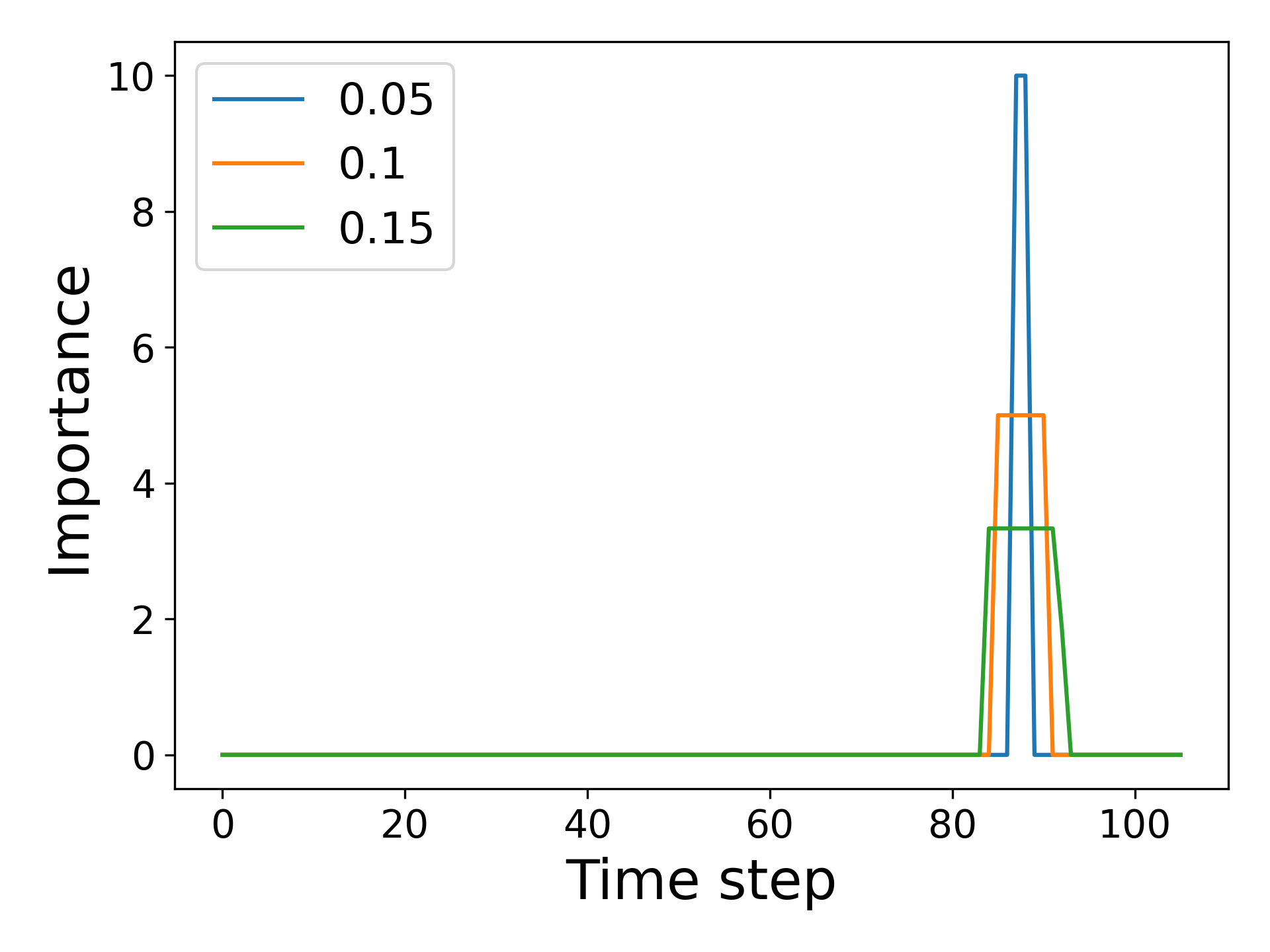
(a) Importance vector of $X_{t}$

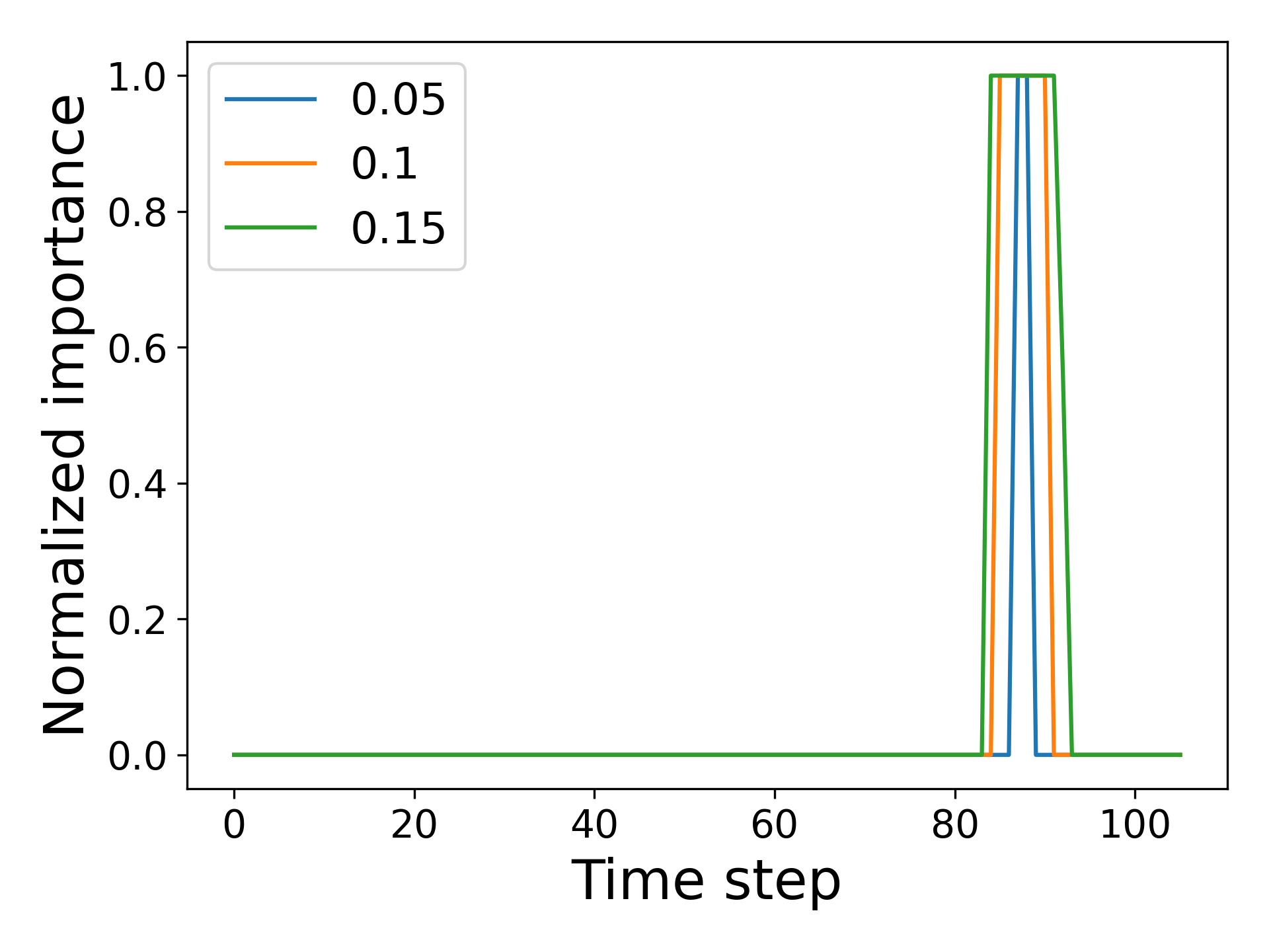
(b) Normalized importance vector of $X_{t}$

Figure 18: Sensitivity analysis on the collision avoidance problem.

B.3 Lunar Lander

Fig. 19 shows the sensitivity analysis on lunar lander and the different color lines correspond to different perturbation amounts. Binary features including left and right leg are not included. The general trend of the result is the same while the value and the exact shape of the curve vary slightly when different $\delta$ is used and our result is robust w.r.t. $\delta$.

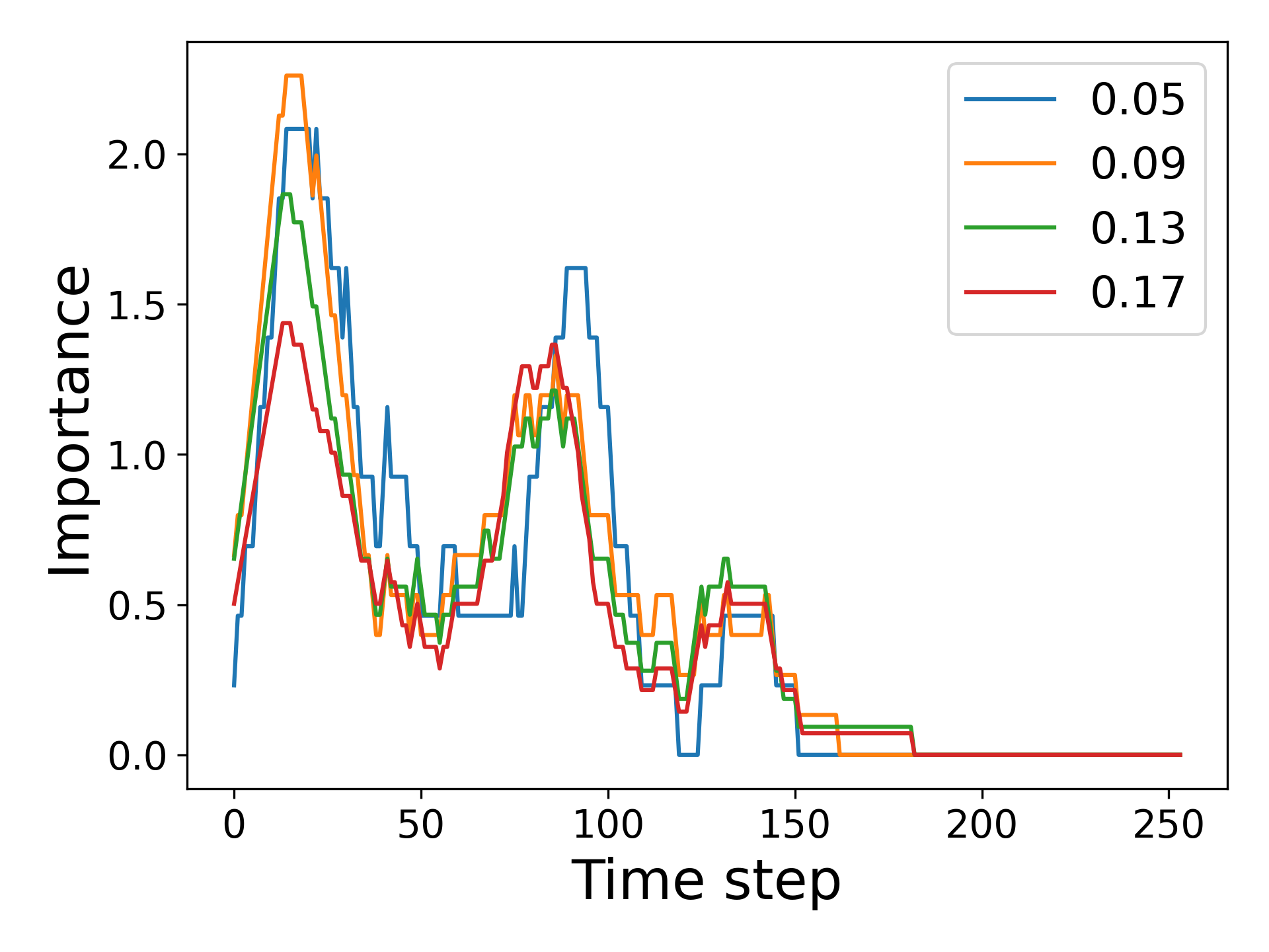
(a) Importance vector of x-position

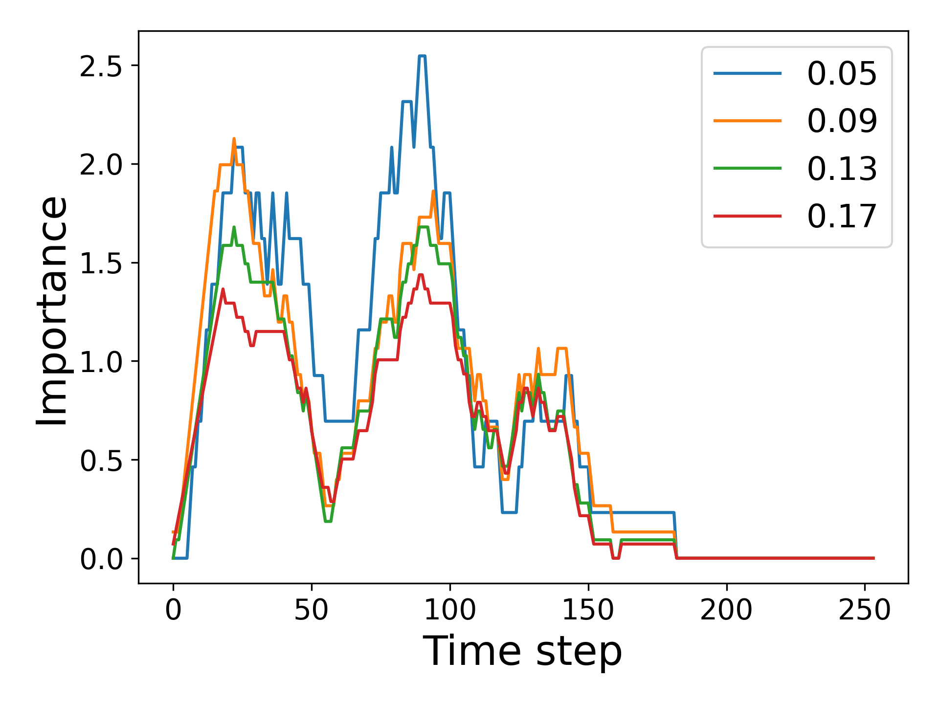
(b) Importance vector of y-position

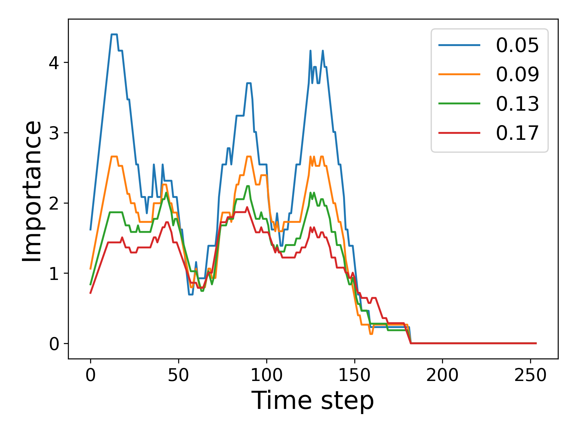
(c) Importance vector of angle

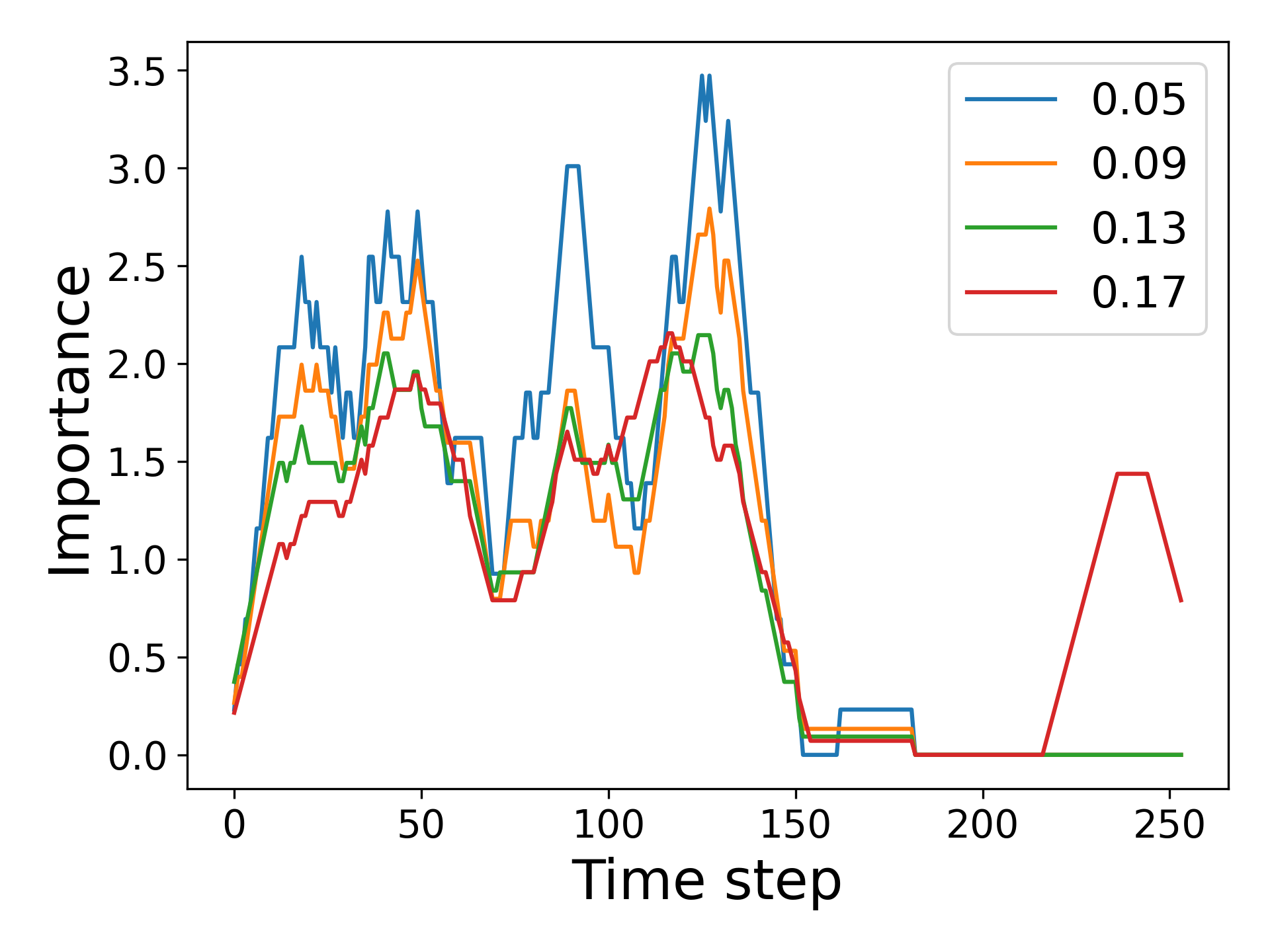
(d) Importance vector of x-velocity

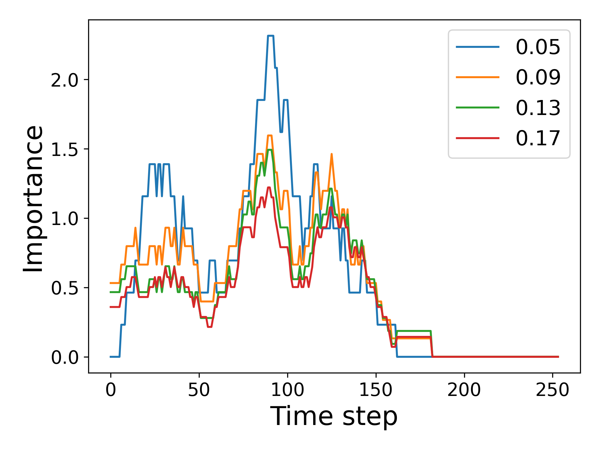
(e) Importance vector of y-velocity

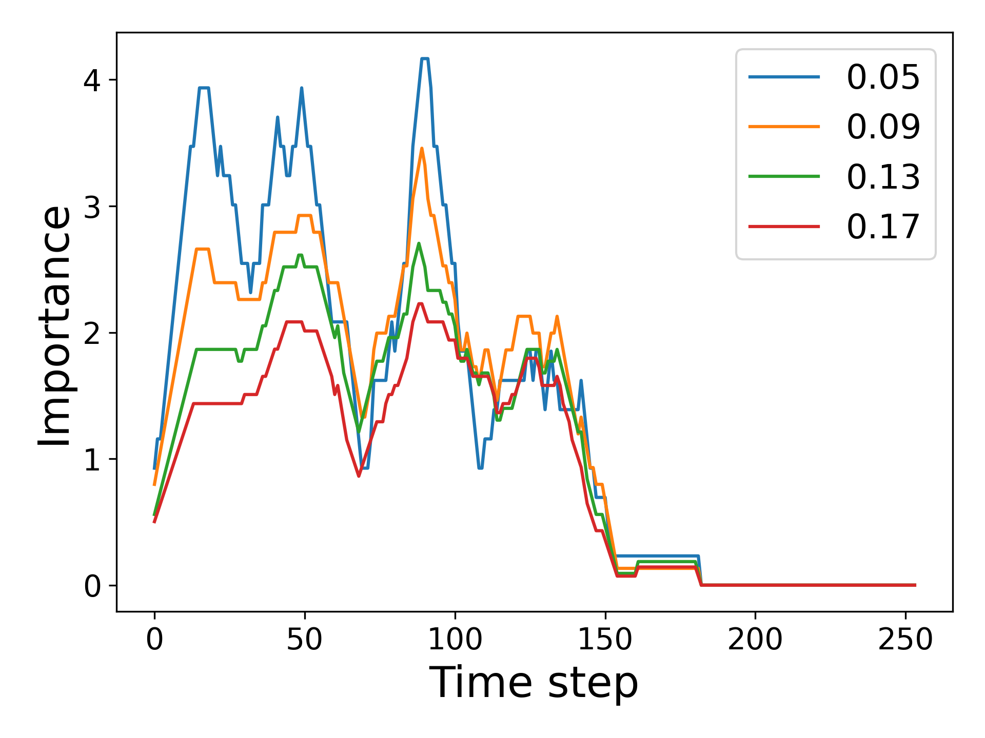
(f) Importance vector of angular velocity

Figure 19: Sensitivity analysis on the lunar lander environment.

B.4 Blackjack

Fig. 20 shows the sensitivity analysis for blackjack, with different color lines representing different perturbation amounts. The binary feature ace is not included. In blackjack, since the smallest legal perturbation amount is one and the range of the value is at most 21, increasing $\delta$ has a much larger effect on the result. However, we can observe that the general shape of the curves is similar, indicating the robustness of our method.

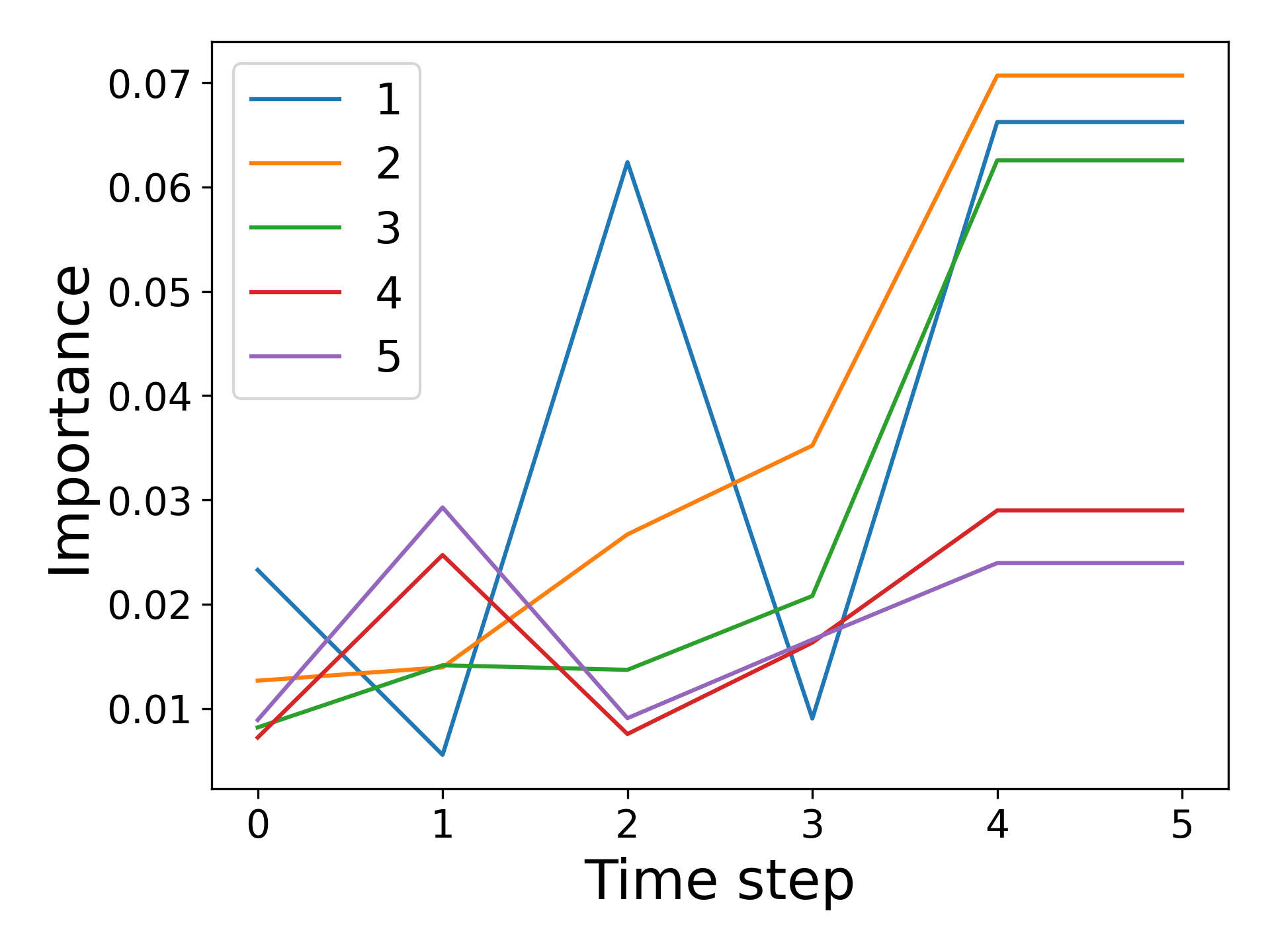
(a) Importance vector of hand

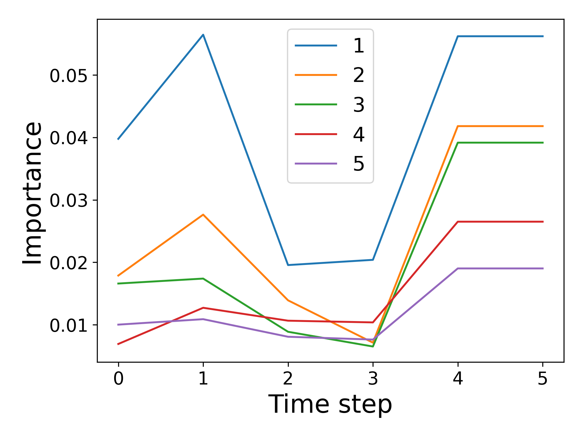
(b) Importance vector of dealer

Figure 20: Sensitivity analysis on the Blackjack environment.

Appendix C Action-based Importance versus Q-value-based Importance

This section discusses the comparison between the action-based importance method and the Q-value-based importance method. It demonstrates that the Q-value-based method sometimes fails to reflect the features in the state that the policy relies on.

Consider a one-step MDP with the SCM shown in Fig. 21, where the state $\mathbf{S}=[S_{1},S_{2}]$, $S_{i}\in[-1,1]$, $i=1,2$, and the action $a\in[-1,1]$. The reward is defined as $R(\mathbf{S},a)=100\times S_{2}+a\times S_{1}$. Under this setting, the optimal policy is:

$$A=\begin{cases}-1&S_{1}<0\\ 1&\text{otherwise}\end{cases}$$

Intuitively, the policy selects the minimum value in the action space when $S_{1}$ is negative , and the maximum value otherwise.

The action-based importance method correctly identifies $S_{1}$ as more important, as the policy only depends on $S_{1}$. However, the Q-value-based method produces a different result. In a one-step MDP, the Q-function is the same as the reward function. As the coefficient in the Q(reward) function is larger for $S_{2}$, the Q-value-based method finds $S_{2}$ more important, which is different from the features that the policy relies on.

Figure 21: The skeleton of SCM of the one step MDP.

References

- Brockman et al. (2016) Brockman, G.; Cheung, V.; Pettersson, L.; Schneider, J.; Schulman, J.; Tang, J.; and Zaremba, W. 2016. Openai gym. arXiv preprint arXiv:1606.01540.
- Bryson (1975) Bryson, A. E. 1975. Applied optimal control: optimization, estimation and control. Boca Raton: CRC Press.
- Byrne (2019) Byrne, R. M. 2019. Counterfactuals in Explainable Artificial Intelligence (XAI): Evidence from Human Reasoning. In IJCAI, 6276–6282.
- Chattopadhyay et al. (2019) Chattopadhyay, A.; Manupriya, P.; Sarkar, A.; and Balasubramanian, V. N. 2019. Neural network attributions: A causal perspective. In International Conference on Machine Learning, 981–990. PMLR.
- Datta, Sen, and Zick (2016) Datta, A.; Sen, S.; and Zick, Y. 2016. Algorithmic transparency via quantitative input influence: Theory and experiments with learning systems. In 2016 IEEE symposium on security and privacy (SP), 598–617. IEEE.
- Gawlikowski et al. (2021) Gawlikowski, J.; Tassi, C. R. N.; Ali, M.; Lee, J.; Humt, M.; Feng, J.; Kruspe, A.; Triebel, R.; Jung, P.; Roscher, R.; et al. 2021. A survey of uncertainty in deep neural networks. arXiv preprint arXiv:2107.03342.
- Glymour, Pearl, and Jewell (2016) Glymour, M.; Pearl, J.; and Jewell, N. P. 2016. Causal inference in statistics: A primer. Hoboken: John Wiley & Sons.
- Greydanus et al. (2018) Greydanus, S.; Koul, A.; Dodge, J.; and Fern, A. 2018. Visualizing and understanding atari agents. In International Conference on Machine Learning, 1792–1801. PMLR.
- Heuillet, Couthouis, and Díaz-Rodríguez (2021) Heuillet, A.; Couthouis, F.; and Díaz-Rodríguez, N. 2021. Explainability in deep reinforcement learning. Knowledge-Based Systems, 214: 106685.
- Hilton (2007) Hilton, D. 2007. Causal explanation: From social perception to knowledge-based causal attribution.
- Hoyer et al. (2008) Hoyer, P.; Janzing, D.; Mooij, J. M.; Peters, J.; and Schölkopf, B. 2008. Nonlinear causal discovery with additive noise models. Advances in neural information processing systems, 21: 689–696.
- Iyer et al. (2018) Iyer, R.; Li, Y.; Li, H.; Lewis, M.; Sundar, R.; and Sycara, K. 2018. Transparency and explanation in deep reinforcement learning neural networks. In Proceedings of the 2018 AAAI/ACM Conference on AI, Ethics, and Society, 144–150.
- Jaiswal et al. (2018) Jaiswal, A.; AbdAlmageed, W.; Wu, Y.; and Natarajan, P. 2018. Bidirectional conditional generative adversarial networks. In Asian Conference on Computer Vision, 216–232. Springer.
- Juozapaitis et al. (2019) Juozapaitis, Z.; Koul, A.; Fern, A.; Erwig, M.; and Doshi-Velez, F. 2019. Explainable reinforcement learning via reward decomposition. In IJCAI/ECAI Workshop on Explainable Artificial Intelligence.
- Kalainathan and Goudet (2019) Kalainathan, D.; and Goudet, O. 2019. Causal discovery toolbox: Uncover causal relationships in python. arXiv preprint arXiv:1903.02278.
- Lopez-Paz et al. (2017) Lopez-Paz, D.; Nishihara, R.; Chintala, S.; Scholkopf, B.; and Bottou, L. 2017. Discovering causal signals in images. In Proceedings of the IEEE conference on computer vision and pattern recognition, 6979–6987.
- Lundberg and Lee (2017) Lundberg, S.; and Lee, S.-I. 2017. A unified approach to interpreting model predictions. arXiv preprint arXiv:1705.07874.
- Madumal et al. (2020) Madumal, P.; Miller, T.; Sonenberg, L.; and Vetere, F. 2020. Explainable reinforcement learning through a causal lens. In Proceedings of the AAAI Conference on Artificial Intelligence, volume 34, 2493–2500.
- Miller (2019) Miller, T. 2019. Explanation in artificial intelligence: Insights from the social sciences. Artificial intelligence, 267: 1–38.
- Mott et al. (2019) Mott, A.; Zoran, D.; Chrzanowski, M.; Wierstra, D.; and Rezende, D. J. 2019. Towards interpretable reinforcement learning using attention augmented agents. arXiv preprint arXiv:1906.02500.
- Olson et al. (2021) Olson, M. L.; Khanna, R.; Neal, L.; Li, F.; and Wong, W.-K. 2021. Counterfactual state explanations for reinforcement learning agents via generative deep learning. Artificial Intelligence, 295: 103455.
- Pearl (2009) Pearl, J. 2009. Causality. Causality: Models, Reasoning, and Inference. Cambridge: Cambridge University Press. ISBN 9780521895606.
- Peters et al. (2014) Peters, J.; Mooij, J. M.; Janzing, D.; and Schölkopf, B. 2014. Causal discovery with continuous additive noise models.
- Puiutta and Veith (2020) Puiutta, E.; and Veith, E. 2020. Explainable reinforcement learning: A survey. In International cross-domain conference for machine learning and knowledge extraction, 77–95. Springer.
- Puri et al. (2019) Puri, N.; Verma, S.; Gupta, P.; Kayastha, D.; Deshmukh, S.; Krishnamurthy, B.; and Singh, S. 2019. Explain your move: Understanding agent actions using specific and relevant feature attribution. arXiv preprint arXiv:1912.12191.
- Ribeiro, Singh, and Guestrin (2016) Ribeiro, M. T.; Singh, S.; and Guestrin, C. 2016. ” Why should i trust you?” Explaining the predictions of any classifier. In Proceedings of the 22nd ACM SIGKDD international conference on knowledge discovery and data mining, 1135–1144.
- Schwab and Karlen (2019) Schwab, P.; and Karlen, W. 2019. Cxplain: Causal explanations for model interpretation under uncertainty. arXiv preprint arXiv:1910.12336.
- Shimizu et al. (2006) Shimizu, S.; Hoyer, P. O.; Hyvärinen, A.; Kerminen, A.; and Jordan, M. 2006. A linear non-Gaussian acyclic model for causal discovery. Journal of Machine Learning Research, 7(10).
- Simonyan, Vedaldi, and Zisserman (2013) Simonyan, K.; Vedaldi, A.; and Zisserman, A. 2013. Deep inside convolutional networks: Visualising image classification models and saliency maps. arXiv preprint arXiv:1312.6034.
- Simonyan, Vedaldi, and Zisserman (2014) Simonyan, K.; Vedaldi, A.; and Zisserman, A. 2014. Deep inside convolutional networks: Visualising image classification models and saliency maps.
- Spirtes et al. (2000) Spirtes, P.; Glymour, C. N.; Scheines, R.; and Heckerman, D. 2000. Causation, prediction, and search. Cambridge: MIT press.
- Sundararajan, Taly, and Yan (2017) Sundararajan, M.; Taly, A.; and Yan, Q. 2017. Axiomatic attribution for deep networks. In International Conference on Machine Learning, 3319–3328. PMLR.
- Sutton and Barto (2018) Sutton, R. S.; and Barto, A. G. 2018. Reinforcement learning: An introduction. Cambridge: MIT press.
- Van Hasselt, Guez, and Silver (2016) Van Hasselt, H.; Guez, A.; and Silver, D. 2016. Deep reinforcement learning with double q-learning. In Proceedings of the AAAI Conference on Artificial Intelligence, volume 30.
- Verma et al. (2018) Verma, A.; Murali, V.; Singh, R.; Kohli, P.; and Chaudhuri, S. 2018. Programmatically interpretable reinforcement learning. In International Conference on Machine Learning, 5045–5054. PMLR.
- Wells and Bednarz (2021) Wells, L.; and Bednarz, T. 2021. Explainable ai and reinforcement learning—a systematic review of current approaches and trends. Frontiers in artificial intelligence, 4: 550030.
- Williams et al. (1989) Williams, J.; Jones, C.; Kiniry, J.; and Spanel, D. A. 1989. The EPIC crop growth model. Transactions of the ASAE, 32(2): 497–0511.
- Yang et al. (2021) Yang, M.; Liu, F.; Chen, Z.; Shen, X.; Hao, J.; and Wang, J. 2021. Causalvae: Disentangled representation learning via neural structural causal models. In Proceedings of the IEEE/CVF conference on computer vision and pattern recognition, 9593–9602.
- Zhang et al. (2021) Zhang, K.; Zhu, S.; Kalander, M.; Ng, I.; Ye, J.; Chen, Z.; and Pan, L. 2021. gcastle: A python toolbox for causal discovery. arXiv preprint arXiv:2111.15155.