$R$-matrix electron-impact excitation data for the H- and He-like ions with $Z=6-30$

Abstract

Plasma models built on extensive atomic data are essential to interpreting the observed cosmic spectra. H-like Lyman series and He-like triplets observable in the X-ray band are powerful diagnostic lines to measure the physical properties of various types of astrophysical plasmas. Electron-impact excitation is a fundamental atomic process for the formation of H-like and He-like key diagnostic lines. Electron-impact excitation data adopted by the widely used plasma codes (AtomDB, CHIANTI, and SPEX) do not necessarily agree with each other. Here we present a systematic calculation of electron-impact excitation data of H-like and He-like ions with the atomic number $Z=6-30$ (i.e., C to Zn). Radiation damped $R$-matrix intermediate coupling frame transformation calculation was performed for each ion with configurations up to $n=6$. We compare the present work with the above three plasma codes and literature to assess the quality of the new data, which are relevant for current and future high-resolution X-ray spectrometers.

1 Introduction

X-ray emitting hot astrophysical plasmas are ubiquitous in the Universe: stellar coronae, supernova remnants, hot plasmas in individual galaxies and galaxy assemblies, and the warm-hot intergalactic media along the cosmic web filaments (Kaastra et al., 2017). When these targets are observed with spectrometer aboard X-ray space observatories (e.g., Chandra, XMM-Newton, and Suzaku), prominent H- and He-like emission lines from various elements (e.g., O and Fe) often stand out above the continuum (e.g., Paerels & Kahn, 2003; Mao et al., 2019). These emission lines are powerful diagnostics tools to constrain the physical properties of the hot astrophysical plasmas, such as temperature, density, elemental abundance, and kinematics.

From the observational perspective, we will soon enter an era with the next generation of X-ray spectrometers, including X-ray Imaging and Spectroscopy Mission (XRISM, Tashiro et al., 2018, to be launched in early 2023), Advanced Telescope for High Energy Astrophysics (Athena, Nandra et al., 2013; Barret et al., 2018, to be launched in the 2030s), Arcus (Smith et al., 2016, proposed in the U.S.), Hot Universe Baryon Surveyor (HUBS, Cui et al., 2020, proposed in China), Super-Diffuse Intergalactic Oxygen Surveyor (Super-DIOS, Yamada et al., 2018, proposed in Japan), Colibrí (Heyl et al., 2019, proposed in Canada), and so on.

We had a taste of the future with the Soft X-ray Spectrometers (SXS, Mitsuda et al., 2014) aboard Hitomi. When observing the hot ($\sim 4.6\times 10^{7}$ K) intracluster media (ICM) of the Perseus galaxy cluster, dozens of emission lines from various ionization stages of cosmic abundant (e.g., Si, Fe, and Ni) and rare (e.g., Cr and Mn) elements are observed. The high-quality line-rich spectrum was used to study the line-of-sight turbulent velocity dispersion (Hitomi Collaboration et al., 2016); the origin of cosmic elements in the ICM (Hitomi Collaboration et al., 2017); the resonance scattering effect of the ICM (Hitomi Collaboration et al., 2018a); and the temperature structure of the ICM (Hitomi Collaboration et al., 2018b).

Astrophysical plasma models play a vital role in interpreting the observed high-resolution X-ray spectra (Raymond, 2005; Kaastra et al., 2008). When modeling hot astrophysical plasmas in the collisional ionized equilibrium (CIE), both the APEC (Smith et al., 2001; Foster et al., 2012) model (and its variants) in XSPEC (Arnaud, 1996) and the CIE model in SPEX Kaastra et al. (1996, 2020) are widely used in the community. CHIANTI (Dere et al., 1997; Del Zanna et al., 2021) can also model CIE plasma and it is widely used in the solar community. All these plasma models are built on an extensive yet ever-expanding atomic database. High-quality X-ray spectra from future missions are challenging the plasma models developed since the 1970s (Landini & Monsignori Fossi, 1970; Mewe, 1972; Raymond & Smith, 1977).

When analyzing the same Hitomi/SXS spectra of Perseus using different plasma models (Hitomi Collaboration et al., 2018c), the measured Fe abundance was found to differ by 16%. The systematic uncertainty due to the instrumental effects (e.g., effective area uncertainty and gain correction factor) is within 15%. The statistical uncertainty is, however, about 1%. That is to say, the power of the instrument is not fully exploited. Theoretical atomic calculations and laboratory measurements of the atomic data (e.g., Betancourt-Martinez et al., 2019, 2020; Gu et al., 2019, 2020; Heuer et al., 2021; Shah et al., 2021) are required to bring the results of plasma diagnostics closer.

In this work, we focus on the electron-impact excitation (EIE) data for H- and He-like ions from C to Zn. Electron-impact excitation is one of the fundamental atomic processes in astrophysical plasmas. During the collision between a free electron and an ion, energy can be transferred from the free electron to a bounded electron in the ion, exciting it to an upper energy level. When the excited electron decays back to the lower level via radiative transition, at least one photon is emitted and contributes to the emission lines in the observed spectra.

2 Diagnostic lines and line power

H-like Lyman series and He-like triplets (Table 1) are the key diagnostic lines to measure the physical properties of astrophysical plasmas. These lines are in general strong in the observed spectra (cf. the review of solar diagnostics Del Zanna & Mason, 2018). Caution that to properly model the observed spectra, dielectronic satellite lines of He-like lines should be included (Dere et al., 2019), which is beyond the scope of this paper.

Table 1: Key diagnostics transitions for H-like and He-like ions.

Label	Lower level	Upper level
Ly$\alpha$ (H-like)	${\rm 1s~{}^{2}S_{1/2}}$	${\rm 2p~{}^{2}P_{3/2,1/2}}$
Ly$\beta$ (H-like)	${\rm 1s~{}^{2}S_{1/2}}$	${\rm 3p~{}^{2}P_{3/2,1/2}}$
Ly$\gamma$ (H-like)	${\rm 1s~{}^{2}S_{1/2}}$	${\rm 4p~{}^{2}P_{3/2,1/2}}$
Ly$\delta$ (H-like)	${\rm 1s~{}^{2}S_{1/2}}$	${\rm 5p~{}^{2}P_{3/2,1/2}}$
He$\alpha$-w (He-like)	${\rm 1s^{2}~{}^{1}S_{0}}$	${\rm 1s~{}2p~{}^{1}P_{1}}$
He$\alpha$-x (He-like)	${\rm 1s^{2}~{}^{1}S_{0}}$	${\rm 1s~{}2p~{}^{3}P_{2}}$
He$\alpha$-y (He-like)	${\rm 1s^{2}~{}^{1}S_{0}}$	${\rm 1s~{}2p~{}^{3}P_{1}}$
He$\alpha$-z (He-like)	${\rm 1s^{2}~{}^{1}S_{0}}$	${\rm 1s~{}2s~{}^{3}S_{1}}$
He$\beta$-w (He-like)	${\rm 1s^{2}~{}^{1}S_{0}}$	${\rm 1s~{}3p~{}^{1}P_{1}}$
He$\gamma$-w (He-like)	${\rm 1s^{2}~{}^{1}S_{0}}$	${\rm 1s~{}4p~{}^{1}P_{1}}$
He$\delta$-w (He-like)	${\rm 1s^{2}~{}^{1}S_{0}}$	${\rm 1s~{}5p~{}^{1}P_{1}}$

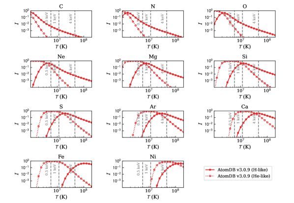
Figure 1: Ionic fraction $(I)$ for cosmic abundant metals in CIE plasmas based on Bryans et al. (2009) as the default of AtomDB v3.0.9. The red solid and dashed lines are for H- and He-like ions, respectively. Vertical gray dashed lines marks the typical temperatures of hot plasmas in individual galaxies ($\sim$0.5 keV, dotted), groups of galaxies ($\sim$1 keV, dashed), and clusters of galaxies ($\sim$4 keV, dot-dashed), respectively.

Lyman series are transitions with $n{\rm p~{}^{2}P_{3/2,1/2}}\rightarrow{\rm 1s~{}^{2}S_{1/2}}~{}(n\geq 2)$. We mainly focus on Ly$\alpha$ ($n=2\rightarrow 1$), Ly$\beta$ ($n=3\rightarrow 1$), Ly$\gamma$ ($n=4\rightarrow 1$), and Ly$\delta$ ($n=4\rightarrow 1$) as they are all available in AtomDB, SPEX, and CHIANTI. For a low-density CIE plasma, the Ly$\alpha$ line (${\rm 2p~{}^{2}P_{3/2,1/2}}\rightarrow{\rm 1s~{}^{2}S_{1/2}}$) should have the highest line power. However, in a high-density CIE plasma, resonance scattering can reduce the intensity of Ly$\alpha$ by scattering a fraction of photons outside our line-of-sight. This will lead to larger ratios of Ly$\beta$/Ly$\alpha$, Ly$\gamma$/Ly$\alpha$, and Ly$\delta$/Ly$\alpha$ than those in a low-density CIE plasma. On the other hand, at the interface between the hot plasma and cold medium, the charge-exchange process can selectively increase the intensity of e.g., Ly$\gamma$ or Ly$\delta$ (Gu et al., 2016). This also leads to a larger ratio of Ly$\beta$/Ly$\alpha$, Ly$\gamma$/Ly$\alpha$, and Ly$\delta$/Ly$\alpha$ than those in a low-density CIE plasma.

He-like triplet refers to the resonance (allowed) ${\rm 1s~{}2p~{}^{1}P_{1}}\rightarrow{\rm 1s^{2}~{}^{1}S_{0}}$, inter-combination (semi-forbidden) ${\rm 1s~{}2p~{}^{3}P_{1,2}}\rightarrow{\rm 1s^{2}~{}^{1}S_{0}}$, and forbidden ${\rm 1s~{}2s~{}^{3}S_{1}}\rightarrow{\rm 1s^{2}~{}^{1}S_{0}}$ transition respectively. The two inter-combination lines are often treated as one line because they are not resolved with current instruments (but will be resolved with future missions). The line ratios among the three are sensitive to plasma temperature and density, external radiation field, and charge-exchange process (Porquet et al., 2010). For a low-density CIE plasma, the resonance line should have the highest line power and the inter-combination line has the lowest line power. In a high-density CIE plasma, on one hand, resonance scattering can reduce the intensity of the resonance line by scattering a fraction of photons outside our line-of-sight (e.g. Sazonov et al., 2002; Xu et al., 2002; Ogorzalek et al., 2017; Hitomi Collaboration et al., 2018c; Chen et al., 2018); on the other hand, the inter-combination line will be stronger and the forbidden line will be weaker because collisional excitation will depopulate the upper level of the forbidden line to those of the intercombination lines (e.g., Porquet et al., 2010). Furthermore, at the interface between the hot plasma and cold medium, the charge-exchange process can increase the forbidden to resonance line ratio (e.g., Branduardi-Raymont et al., 2007; Zhang et al., 2014; Gu et al., 2016). Similarly, the line ratio of the He$\alpha$ triplets can also be different from collisionally ionized equilibrium plasma due to photo-excitation (e.g., Porquet et al., 2010). Higher-order resonance (allowed) ${\rm 1s}~{}n{\rm p~{}^{1}P_{1}}\rightarrow{\rm 1s^{2}~{}^{1}S_{0}}$ with $n=3-5$ can also be present in high-quality spectra of future missions, while other higher-order He-like lines are less observable.

For each optically thin emission line in a CIE plasma, its strength can be described by line power $P_{ji}$ (in photons per unit time and volume):

$$P_{ji}(T,~{}n_{\rm H})=A_{ji}~{}n_{\rm H}~{}A(Z)~{}I(T,~{}n_{\rm H})~{}N_{j}(T,~{}n_{\rm H}),$$ (1)

where $A_{ji}$ is the spontaneous transition probability from the upper level $j$ to the lower level $i$, $n_{\rm H}$ the hydrogen number density of the plasma, $A(Z)$ the elemental abundance with respect to hydrogen, $Z$ the atomic number, $I$ the normalized ionic fraction (the sum of all the ionization stages of the same element is unity), and $N_{j}$ the normalized level population of the upper level $j$ (the sum of all the levels is unity). While the $A$-value is independent of the plasma temperature, both the ionic fraction ($I$) and level population ($N_{j}$) depend on the plasma temperature and density.

Elemental abundances $A(Z)$ are often given in units of solar abundance and there are quite a few of solar abundance tables available to use. Generally speaking, C, N, O, Ne, Mg, Si, S, Ar, Ca, Fe and Ni are the relatively abundant ones for $Z\geq 6$ (Anders & Grevesse, 1989; Asplund et al., 2009; Lodders et al., 2009).

Ionic fraction $(I)$ is usually taken from pre-calculated ionization balance tables, which only depend on the temperature of low-density CIE plasma (Fig. 1). The default ionization balance is Bryans et al. (2009) for APEC, Dere et al. (2009) for CHIANTI, and Urdampilleta et al. (2017) for SPEX. Around the peak ionic fraction temperatures, the ionic fraction agrees within a few percent among the three codes. At both higher and lower temperature ends when the ionic fraction is rather small, larger deviations ($\gtrsim 20$%) can be found. We caution that metastable levels will start to be populated as the plasma density increases, which can modify the ionization balance significantly (Dufresne & Del Zanna, 2019; Dufresne et al., 2020, 2021).

The user can choose which ionization balance and solar abundance table to use in pyatomdb, ChiantiPy, and SPEX. When comparing plasma models, it is better to use the same solar abundance and ionization balance tables.

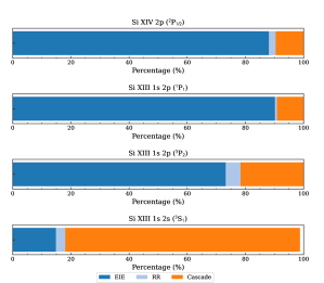
Figure 2: Percentage contribution of the atomic processes to the level population of Si xiv and Si xiii in a CIE plasma with $kT=1$ keV. The four levels, from top to bottom, are the upper levels of Ly$\alpha$, He$\alpha$-w, He$\alpha$-x, and He$\alpha$-z. Contributions from the electron-impact excitation (EIE), radiative recombination (RR), and cascade are shown in dark blue, light blue, and orange. The SPEX code (v3.06.01) is used to calculate the level population here.

The level population ($N_{j}$) depends on various atomic processes. Figure 2 illustrates the percentage contribution of the atomic processes to the level population of Si xiv and Si xiii for a CIE plasma with $kT=1$ keV. Similar results can be found for other H- and He-like ions in CIE plasmas. Generally speaking, electron-impact excitation (EIE) contributes most to the upper level population of resonance lines. Radiative recombination (RR) has a minor contribution to the level population. Note that the same RR data, sourced from Badnell (2006), are implemented via interpolation for AtomDB and CHIANTI or parameterization (Mao & Kaastra, 2016) for SPEX. The contribution from cascade is negligible for resonance lines but it can be crucial for forbidden lines (Hitomi Collaboration et al., 2018c).

3 Status quo

We examine electron-impact excitation data in the latest versions of AtomDB (v3.0.9), CHIANTI (v10.0.1), and SPEX (v3.06.01). The electron-impact excitation data of the key diagnostics line (Table 1) are sourced differently in the three atomic databases. For H-like ions, AtomDB mainly adopts the distorted waves data (with the independent process and isolated resonances approximation) of Li et al. (2015) for elements heavier and including Al. For lighter elements, either $R$-matrix data (Ballance et al., 2003) or distorted wave calculation by A. Foster with the Flexible Atomic Code (FAC, Gu, 2008) are used. For CHIANTI and SPEX, $R$-matrix data are used for a few ions. Interpolation or extrapolation along the iso-electronic sequence is used for the rest of the H-like ions. Table 2 provides a summary of the source of the electron-impact excitation data of the Ly$\alpha$ to Ly$\delta$ transitions in the three atomic databases.

Table 2: Source of the electron-impact excitation data of the H-like Ly$\alpha$ to Ly$\delta$ transitions in SPEX v3.06.01, AtomDB v3.0.9, and CHIANTI database v10.0.1. DW and RM are short for distorted wave and $R$-matrix calculations, respectively.

Ion	SPEX	AtomDB	CHIANTI
C vi	Aggarwal & Kingston (1991a, RM)	Ballance et al. (2003, RM)	Ballance et al. (2003, RM)
N vii	Interpolation	FAC (DW)	Interpolation
O viii	Interpolation	Ballance et al. (2003, RM)	Ballance et al. (2003, RM)
Ne x	Aggarwal & Kingston (1991b, RM), DW for Ly$\beta$	Ballance et al. (2003, RM)	Ballance et al. (2003, RM)
Na xi	Interpolation	FAC (DW)	Interpolation
Mg xii	Interpolation	FAC (DW)	Interpolation
Al xiii	Interpolation	Li et al. (2015, DW)	Interpolation
Si xiv	Aggarwal & Kingston (1992a, RM)	Li et al. (2015, DW)	Aggarwal & Kingston (1992a, RM)
P xv	Interpolation	Li et al. (2015, DW)	Interpolation
S xvi	Interpolation	Li et al. (2015, DW)	Interpolation
Cl xvii	Interpolation	Li et al. (2015, DW)	Interpolation
Ar xviii	Interpolation	Li et al. (2015, DW)	Interpolation
K xix	Interpolation	Li et al. (2015, DW)	Interpolation
Ca xx	Aggarwal & Kingston (1992b, RM)	Li et al. (2015, DW)	Aggarwal & Kingston (1992b, RM)
Cr xxiv	Interpolation	Li et al. (2015, DW)	– –
Mn xxv	Interpolation	Li et al. (2015, DW)	– –
Fe xxvi	Kisielius et al. (1996, RM), interpolation for Ly${\delta}$	Li et al. (2015, DW)	Ballance et al. (2002, RM)
Ni xxviii	Extrapolation	Li et al. (2015, DW)	Extrapolation

For He-like ions, AtomDB mainly adopts $R$-matrix data (including the radiation damping effect) for all the levels up to $n=5$: Whiteford et al. (2001) for He-like Fe xxv and Whiteford (2005) for other He-like ions. The latter ones, available on OPEN-ADAS, were calculated following Whiteford et al. (2001, for He-like Ar and Fe only) with some modifications (given in the comment section of the data files). These data are not validated (e.g., comparing to previous calculations) in a peer-reviewed journal publication as the lead author left the field before finishing the project. In particular, He-like Fe xxv data of Whiteford (2005) is not consistent with that of Whiteford et al. (2001). This is described in Sect. 5 later. CHIANTI also uses a large fraction of these data (Whiteford, 2005). But it uses the $R$-matrix data (without the radiation damping effect) of Aggarwal et al. (2009) for Na x and interpolation along the iso-electronic sequence for P xiv and K xviii. SPEX adopts the Coulomb-Born-Exchange data of Sampson et al. (1983), which ignored resonances.

Table 3: Source of the electron-impact excitation data of the He-like triplet transitions in SPEX v3.06.01, AtomDB v3.0.9, and CHIANTI database v9.0.1. Sampson et al. (1983) and Whiteford (2005) used Coulomb-Born-Exchange and $R$-matrix methods, respectively.

Ion	SPEX	AtomDB	CHIANTI
C v	Sampson et al. (1983, CBE)	Whiteford (2005, RM)	Interpolation
N vi	Sampson et al. (1983, CBE)	Whiteford (2005, RM)	Interpolation
O vii	Sampson et al. (1983, CBE)	Whiteford (2005, RM)	Whiteford (2005, RM)
Ne ix	Sampson et al. (1983, CBE)	Whiteford (2005, RM)	Whiteford (2005, RM)
Na x	Sampson et al. (1983, CBE)	Whiteford (2005, RM)	Aggarwal et al. (2009)
Mg xi	Sampson et al. (1983, CBE)	Whiteford (2005, RM)	Whiteford (2005, RM)
Al xii	Sampson et al. (1983, CBE)	Whiteford (2005, RM)	Whiteford (2005, RM)
Si xiii	Sampson et al. (1983, CBE)	Whiteford (2005, RM)	Whiteford (2005, RM)
P xiv	Sampson et al. (1983, CBE)	Whiteford (2005, RM)	Interpolation
S xv	Sampson et al. (1983, CBE)	Whiteford (2005, RM)	Whiteford (2005, RM)
Cl xvi	Sampson et al. (1983, CBE)	Whiteford (2005, RM)	Interpolation
Ar xvii	Sampson et al. (1983, CBE)	Whiteford (2005, RM)	Whiteford (2005, RM)
K xviii	Sampson et al. (1983, CBE)	Whiteford (2005, RM)	Interpolation
Ca xix	Sampson et al. (1983, CBE)	Whiteford (2005, RM)	Whiteford (2005, RM)
Cr xxiii	Sampson et al. (1983, CBE)	Whiteford (2005, RM)	Whiteford (2005, RM)
Mn xxiv	Sampson et al. (1983, CBE)	Whiteford (2005, RM)	– –
Fe xxv	Sampson et al. (1983, CBE)	Whiteford et al. (2001, RM)	Whiteford (2005, RM)
Ni xxvii	Sampson et al. (1983, CBE)	Whiteford (2005, RM)	Whiteford (2005, RM)

Electron-impact excitation data are usually provided in the form of dimensionless effective collisional strength $\Upsilon_{ij}$). This is obtained by convolving the ordinary collision strength ($\Omega_{ij}$) with the Maxwellian distribution:

$$\Upsilon_{ij}=\int_{0}^{\infty}\Omega_{ij}~{}\exp\left(-\frac{E_{f}}{kT}\right)~{}d\left(\frac{E_{f}}{kT}\right)~{},$$ (2)

where $E_{f}$ is the scattered electron energy, $k$ the Boltzmann constant, and $T$ the electron temperature of the plasma. Effective collisional strength are usually tabulated on a narrow or wide temperature grid, depending on the original calculations. Interpolation among these temperatures and extrapolation beyond the temperature range are implemented by AtomDB and CHIANTI. For SPEX, the collision data as a function of temperature are implemented via parameterization to cover a wide temperature range (Kaastra et al., 2008).

We caution that the energy levels and spontaneous transition rate (i.e., $A$-values) among these three atomic databases do not necessarily agree. Detailed comparisons are given in Appendix A.

4 $R$-matrix calculation

Here we present a systematic $R$-matrix calculation for H- and He-like ions. $R$-matrix intermediate coupling frame transformation calculation (ICFT Griffin et al., 1998) including the effect of radiation damping (Robicheaux et al., 1995; Gorczyca & Badnell, 1996) was performed for each ion with configurations up to $n=6$. That is to say, 36 levels for H-like ions and 71 levels for He-like ions.

We used the AUTOSTRUCTURE code (Badnell, 2011) to calculate the target atomic structure. Wave functions were obtained by diagonalizing the Breit-Pauli Hamiltonian (Eissner et al., 1974). We include one-body relativistic terms (mass-velocity, nuclear plus Blume & Watson spin-orbit, and Darwin) perturbatively. The Thomas-Fermi-Dirac-Amaldi model was used for the electronic potential with $nl$-dependent scaling parameters (Nussbaumer & Storey, 1978). We set the $nl$-dependent scaling parameters to unity, following Ballance et al. (2002) and Malespin et al. (2011).

For the scattering calculation, we used radiation damped $R$-matrix ICFT method. We used 110 continuum basis orbitals for H- and He-like ions with configurations up to $n=6$ to cover the energy range from the ground state to $\gtrsim 6~{}I_{p}$, where $I_{p}$ is the ionization threshold. This ensures the cross section is close to the asymptotic limit before extrapolating to the infinite limit point.

Angular momenta up to $2J=26$ and $2J=96$ were included for the exchange and non-exchange calculations, respectively. Higher angular momenta (up to infinity) were included following the top-up formula of the Burgess sum rule (Burgess, 1974) for dipole-allowed transitions and a geometric series for the non-dipole-allowed transitions (Badnell & Griffin, 2001).

The outer-region exchange calculation of the resonance region used a rather fine energy mesh with the number of sampling points ranges from $\sim 1.0\times 10^{5}$ for H-like C vi to $\sim 5.8\times 10^{5}$ for H-like Zn xxx and from $\sim 0.8\times 10^{5}$ for He-like C v to $5.6\times 10^{5}$ for He-like Zn xxxix. Beyond the resonance regions (up to six times the ionization potential), the outer-region exchange calculations were performed with a coarse energy mesh with $\sim 2500$ sampling points. A similar coarse energy mesh was also used for the outer-region non-exchange calculations.

To complete the Maxwellian convolution (Eq. 2) at high temperatures, we calculated the infinite-energy Born and dipole line strength limits using AUTOSTRUCTURE. Between the last calculated energy point and the two limits, interpolation was used according to the type of transition in the Burgess–Tully scaled domain (i.e. the quadrature of the reduced collision strength over reduced energy; see Burgess & Tully, 1992).

5 Results

We have obtained radiation damped $R$-matrix electron-impact excitation data for the H- and He-like iso-electronic sequence with $Z=6-30$, where $Z$ is the atomic number, e.g., $Z=14$ for silicon. Our effective collision strengths cover four orders of magnitude in temperature $(z+1)^{2}(2\times 10^{2},~{}2\times 10^{6})~{}{\rm K}$, where $z$ is the ionic charge (e.g., $z=10$ for He-like Mg xi).

Effective collision strength data are archived according to the Atomic Data and Analysis Structure (ADAS) data class adf04 and are available on Zenodo DOI: 10.5281/zenodo.7226828. Optimal interval-averaged ordinary collision strength data are also provided, which can be used for convolution with non-Maxwellian distributions. The ordinary collision strength data files are produced with the latest version of adasexj. For each transition, the number of bins (or intervals) is around 100, depending on the width of the resonance region. Moreover, the Zenodo package also includes the input files of the $R$-matrix calculations, binned ordinary collision strength data (in the adf04 format), atomic data and python scripts used to create the figures presented in this manuscript. These data will be used to improve the atomic databases of astrophysical plasma codes, such as AtomDB (Smith et al., 2001; Foster et al., 2012), CHIANTI (Dere et al., 1997; Del Zanna et al., 2021), and SPEX (Kaastra et al., 1996, 2020).

6 Discussion

A scattering calculation using the $R$-matrix ICFT method (Sect. 4) necessarily uses the Breit–Pauli R-matrix structure code. This includes only one-body relativistic operators (excluding QED). In addition, it requires the user to supply a unique set of non-relativistic orthogonal radial orbitals from an external atomic structure code. Our atomic structure calculated with AUTOSTRUCTURE for subsequent $R$-matrix scattering calculations is denoted as AS-RM. When compared with other structure calculations (including AUTOSTRUCTURE) which make use of two-body relativistic operators and/or QED and/or non-unique and/or non-orthogonal relativistic orbitals, the AS-RM level energies and A-values are less accurate. For the upper levels of the key diagnostic transitions (Table 1), the AS-RM level energies can differ up to $\sim 0.05$ % for H-like and $\sim 0.23$ % for He-like when compared to the three atomic databases (Appendix A). Similarly, by $n=5$ the AS-RM A-values can differ by up to $\sim 25$ % for H-like and $\sim 40$ % for He-like while the A-values of the key transitions among the three databases differ by up to $\sim 5$ % for H-like and $\sim 40$ % (Appendix A). More accurate level energies and A-values than the AS-RM ones can be obtained from AUTOSTRUCTURE as described in Appendix A and we denote them AS-REL. Other sources include Aggarwal et al. (2009, 2010); Aggarwal & Keenan (2010, 2012a, 2012b, 2013); Malespin et al. (2011).

In this section, we compare the effective collisional strength of the key diagnostic lines in Table 1 among the present work, all three atomic databases (AtomDB, CHIANTI, and SPEX), and some reference results not incorporated in the three atomic databases. We focus on the following representative elements: Fe (Sect. 6.1), Ca (Sect. 6.2), Si (Sect. 6.3), and O (Sect. 6.4). We also show exemplary impacts on observations (Sect. 6.5).

6.1 Fe xxvi and Fe xxv

As shown in Figure 3, the effective collision strength of the Lyman series agrees $\lesssim 5$ % for Ly$\alpha$ and $\lesssim 20$ % for Ly$\beta$ to Ly$\delta$ among the present work, AtomDB, CHIANTI, and Aggarwal & Keenan (2013). Ly$\alpha$ to Ly$\gamma$ data in SPEX can differ by $\gtrsim 50$ % from the other data sets at $T>10^{7}$ K. The original Dirac $R$-matrix calculation by Kisielius et al. (1996) was performed at $T=10^{6-7.5}$ K. Hence, the root of the difference is in the extrapolation at $T>10^{7.5}$ K in SPEX. Ly$\delta$ in SPEX is obtained from interpolation along the isoelectronic sequence (Table 3), which is systematically higher (up to $\sim 20$ %) than the present work.

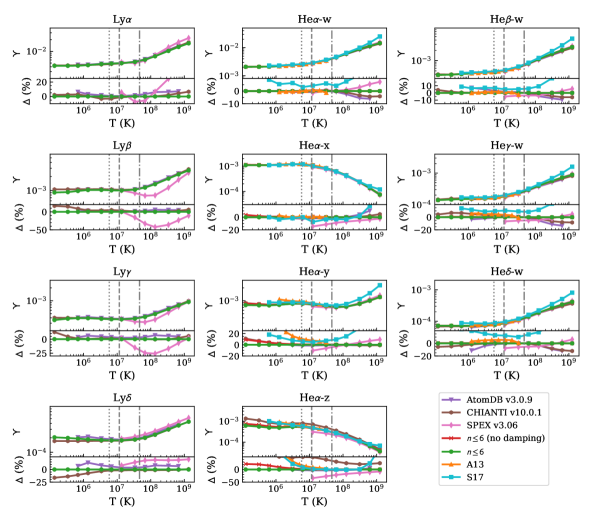
Figure 3: Comparison of effective collisional strength data of key diagnostic lines for Fe xxvi and Fe xxv. AtomDB, CHIANTI, and SPEX data are shown in purple (triangle down), brown (triangle down), and magenta (triangle down), respectively. Present work without radiation damping, present work with radiation damping, Aggarwal & Keenan (2013), and Si et al. (2017) are shown in red (x)

, green (circle), orange (triangle up), and cyan (square), respectively. Percentage difference ($\Delta$) is given with respect to the present work. Vertical dashed lines mark typical temperatures of hot plasmas in individual galaxies ($\sim 0.5$ keV, dotted), groups of galaxies ($\sim 1$ keV, dashed), and clusters of galaxies ($\sim 4$ keV, dot-dashed), respectively. When the ionic fraction is too low (Fig. 1), SPEX skipped the level population calculation (including the effective collisional strength data) for computational efficiency.

For the He$\alpha$-w (resonance) line, all $R$-matrix data agree $\lesssim 3$ % at $T<10^{8}$ K. Distorted wave data (with independent process and isolated resonances approximation, IPIRDW) from Si et al. (2017) is systematically higher by a few percent. Such offset is also shown in the Figure 2 of Si et al. (2017), where the authors calculated both IPIRDW and Dirac $R$-matrix data. The offset is due to the different treatment of resonances by the two calculations, which is illustrated in Figure 1 of Si et al. (2017). At $T>10^{8}$ K, IPIRDW data by Si et al. (2017) increases more rapidly than the $R$-matrix data. The difference originates from the convolution of Maxwellian (Eq. 2) at high temperatures (cf. Sect. 4 and Si et al., 2017). The comparison of He$\beta$ to He$\delta$ resonance transitions among different data sets share similar issues found for He$\alpha$.

For the He$\alpha$-x (intercombination) line, all $R$-matrix data agree $\lesssim 3$ % at $T<10^{8}$ K. IPIRDW data from Si et al. (2017) agrees $\lesssim 8$ %. For the He$\alpha$-y (intercombination) line, relatively large differences ($\lesssim 25$ %) can be found among different data sets at $T<10^{7}$ K. The present work and Whiteford et al. (2001, used by AtomDB) agree $\lesssim 3$ % at $T\sim 10^{6-7}$ K (the latter does not calculate below $\sim 10^{6}$ K). Whiteford (2005) covers one order of magnitude lower in temperature than Whiteford et al. (2001) but differs by up to $\sim 15$ %. Between Si et al. (2017) and Aggarwal & Keenan (2013), the former is relatively lower (see also Figure 2 of Si et al., 2017). At $T=5.8\times 10^{6}$ K (or 0.5 keV), Aggarwal & Keenan (2013) is larger by $\sim 12$ % than the present work.

Similarly, large differences are found below $5.8\times 10^{6}$ K for the He$\alpha$-z (forbidden) line. Furthermore, Whiteford (2005) data is systematically above ($\gtrsim 20$ %) all other calculations at $T\lesssim 10^{8}$ K. At $T\sim 10^{6}$ K, Whiteford (2005) is larger than both Whiteford et al. (2001) and the present work by $\sim 50$ %. Such a large difference cannot be explained by the radiation damping effect, which is $\lesssim 20$ % at low temperatures and has no impact at higher temperatures (Figure 3).

For both He$\alpha$-y and z lines, Aggarwal & Keenan (2013) and Si et al. (2017) data are larger ($\gtrsim 10$ %) than the present work at $T\lesssim 5.8\times 10^{6}$ K (or T$\lesssim 0.5$ keV). On the one hand, radiation damping is not included in Aggarwal & Keenan (2013). On the other hand, all the calculations are subject to the inherent lack of convergence in the target configuration-interaction expansion and/or the collisional close-coupling expansion for weaker transitions (Fernández-Menchero et al., 2017; Del Zanna et al., 2019). Note that, under CIE conditions, the ionic fraction of Fe xxv at $T\lesssim 0.5$ keV is more than three orders of magnitude lower than the peak value (Figure 1).

6.2 Ca xx and Ca xix

As shown in Figure 4, the effective collision strengths of the Lyman series agree $\lesssim 10$ % for Ly$\alpha$ to Ly$\delta$ lines between the present work and Aggarwal & Kingston (used by CHIANTI and SPEX 1992b). Similar good agreement is found between the present work and Li et al. (2015, used by AtomDB) at $T\gtrsim 10^{7}$ K. At lower temperatures, relatively larger differences (up to $\sim 20$ %) can be found.

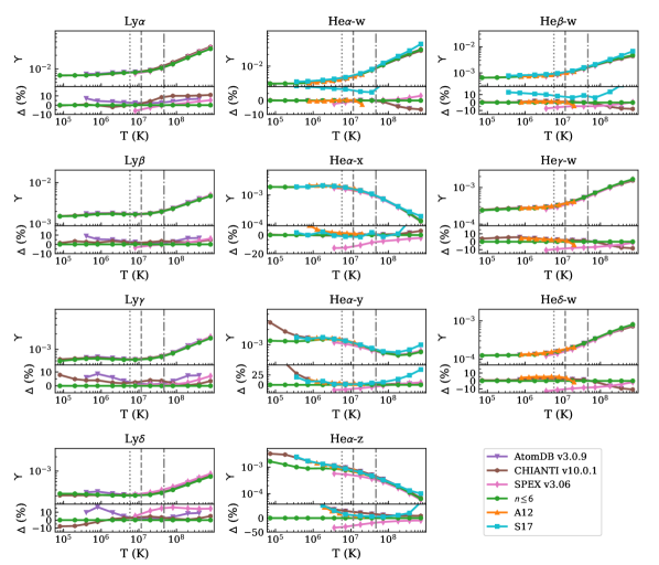
Figure 4: Comparison of effective collisional strength data of key diagnostic lines for Ca xx and Ca xix. AtomDB, CHIANTI, and SPEX data are shown in purple (triangle down), brown (hexagon), and magenta (diamond), respectively. Present work, Aggarwal & Keenan (2012b), and Si et al. (2017) are shown in green (circle), orange (triangle up), and cyan (square), respectively. Percentage difference ($\Delta$) is given with respect to the present work. Vertical dashed lines mark typical temperatures of hot plasmas in individual galaxies ($\sim 0.5$ keV, dotted), groups of galaxies ($\sim 1$ keV, dashed), and clusters of galaxies ($\sim 4$ keV, dot-dashed), respectively. When the ionic fraction is too low (Fig. 1), SPEX skipped the level population calculation (including the effective collisional strength data) for computational efficiency.

For the He$\alpha$-w (resonance) line, all $R$-matrix data agree $\lesssim 3$ % at $T<10^{8}$ K except CHIANTI at $T\gtrsim 10^{8}$ K. The original $R$-matrix data from Aggarwal & Keenan (2012b) is calculated up to $10^{7.4}$ K. The high-temperature extrapolation in CHIANTI might be the issue. IPIRDW data from Si et al. (2017) is systematically higher by $\gtrsim 5$ %, similar to Fe xxv (Sect. 6.1). For the He$\alpha$-x (intercombination) line, the Sampson et al. (1983) data (used by SPEX) stands out at $T\sim 10^{7-8}$ K but it is still within $\sim 20$ %. For the He$\alpha$-y (intercombination) line, large differences ($\gtrsim 25$ %) can be found between the present work and Whiteford (2005, used by AtomDB and CHIANTI) at $T\lesssim 10^{6}$ K. Even larger differences can be found for the He$\alpha$-z line at $T\lesssim 10^{6}$ K, although the ionic fraction of Ca xix at $T\lesssim 10^{6.2}$ K is more than three orders of magnitude lower than the peak value under CIE conditions (Figure 1). Again, Whiteford (2005) is larger than the present work by $\sim 10$ % at high temperatures ($T\gtrsim 10^{8}$ K). For He$\beta$ lines, the SPEX He$\beta$-z data is again systematically larger than all other calculations at $T\gtrsim 10^{7}$ K.

The comparison of He$\beta$ to He$\delta$ resonance transitions among different data sets share similar issues found for He$\alpha$-w with one caveat. The He$\gamma$-w and He$\delta$-w data in Si et al. (2017) are systematically lower by one to three orders of magnitude (beyond the plotting frame of Fig. 4) when compared to all the $R$-matrix data.

6.3 Si xiv and Si xiii

As shown in Figure 5, Ly$\alpha$ to Ly$\delta$ agree $\lesssim 5$ % among all $R$-matrix data sets, while the IPIRDW data from Li et al. (2015) show relatively large (but still within $\sim 25$ %) differences. The high-temperature extrapolation by CHIANTI and SPEX above $10^{6.4}$ K (Aggarwal & Kingston, 1992a) might explain the difference noticed here.

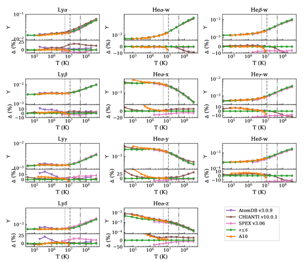
Figure 5: Comparison of effective collisional strength data of key diagnostic lines for Si xiv and Si xiii. AtomDB, CHIANTI, and SPEX data are shown in purple (triangle down), brown (triangle down), and magenta (triangle down), respectively. Present work and Aggarwal & Keenan (2010) are shown in green (circle) and orange (triangle up), respectively. Percentage difference ($\Delta$) is given with respect to the present work. Vertical dashed lines mark typical temperatures of hot plasmas in individual galaxies ($\sim 0.5$ keV, dotted), groups of galaxies ($\sim 1$ keV, dashed), and clusters of galaxies ($\sim 4$ keV, dot-dashed), respectively. When the ionic fraction is too low (Fig. 1), SPEX skipped the level population calculation (including the effective collisional strength data) for computational efficiency.

For He$\alpha$ and He$\delta$ lines, apart from similar issues discussed above, we notice the relatively large ($\gtrsim 20$ %) increase of Whiteford (2005, used by CHIANTI) at $T>10^{8}$ K for He$\alpha$-y line. There is no high-temperature extrapolation here because the original calculation goes to $4.5\times 10^{8}$ K. At such a high temperature, the ionic fraction of Si xiii is more than three orders of magnitude lower than the peak value under CIE conditions (Figure 1).

6.4 O viii and O vii

The effective collision strengths of the Lyman series agree $\lesssim 5$ % for Ly$\alpha$ and Ly$\beta$ and $\lesssim 10$ % for Ly$\gamma$ and Ly$\delta$ among the present work, AtomDB, CHIANTI, and Aggarwal et al. (2010). The original data of Ballance et al. (2003) was calculated up to $1.8\times 10^{7}$ K. At this boundary temperature, the Ballance et al. (2003) data is lower $\lesssim 5$ % than the present work. This smaller difference is likely due to the coverage of scattering energy in the two calculations. Ballance et al. (2003) used 70 continuum basis orbitals to cover at least $\sim 4.5$ times the ionization potential of O viii. In the present work, we used 110 continuum basis orbitals to cover at least $\sim 6.2$ times the ionization potential. As shown in Figure 3 of Malespin et al. (2011), covering a wider energy range can better constrain the high-temperature effective collision strength. At $T\gtrsim 1.8\times 10^{7}$ K, AtomDB and CHIANTI extrapolated the high-temperature data differently. In addition, the SPEX Ly$\beta$ data is systematically lower than the present work by $\gtrsim 10$ % at $T\lesssim 10^{8}$ K.

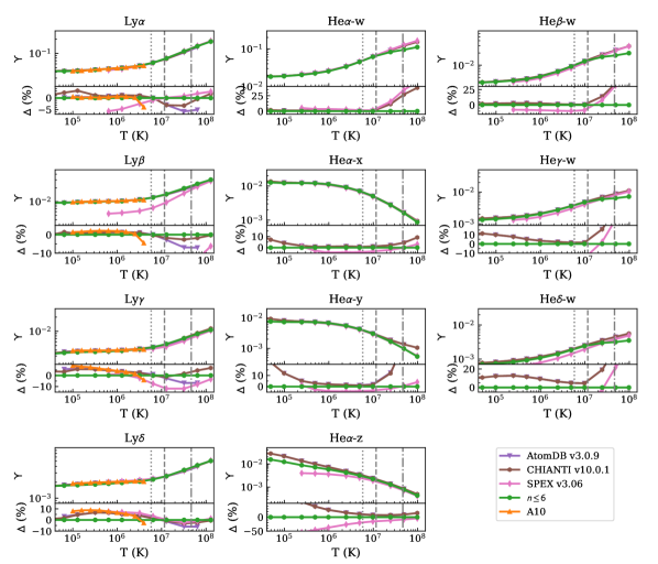
Figure 6: Comparison of effective collisional strength data of key diagnostic lines for O viii and O vii. AtomDB, CHIANTI, and SPEX data are shown in purple (triangle down), brown (triangle down), and magenta (triangle down), respectively. Present work and Aggarwal et al. (2010) are shown in green (circle) and yellow (triangle up), respectively. Percentage difference ($\Delta$) is given with respect to the present work. Vertical dashed lines mark typical temperatures of hot plasmas in individual galaxies ($\sim 0.5$ keV, dotted), groups of galaxies ($\sim 1$ keV, dashed), and clusters of galaxies ($\sim 4$ keV, dot-dashed), respectively. When the ionic fraction is too low (Fig. 1), SPEX skipped the level population calculation (including the effective collisional strength data) for computational efficiency.

More than $\sim 10$ % differences are found between the present work and Whiteford (2005) for the resonance and intercombination lines at $T\gtrsim 4\times 10^{7}$ K. Under CIE conditions, the ionic fraction of O vii at $T\gtrsim 10^{7}$ K is more than three orders of magnitude lower than the peak value (Figure 1). For the forbidden line (He$\alpha$-z), $\gtrsim 10$ % difference is noticed at $T<10^{6}$ K, where the ionic fraction of O vii peaks. This temperature is less relevant for studies of individual galaxies and galaxy assemblies, but it might be relevant for stellar coronae.

6.5 Exemplary impact to observations

As mentioned earlier, a relatively large difference ($\gtrsim 10$ % for $T\lesssim 10^{8}$ K) is found between the present work and SPEX v3.06.01 for O viii Ly$\beta$, which is less affected by resonance scattering than Ly$\alpha$. Here we show simulated spectra representative of two next-generation high-resolution X-ray spectrometers: HUBS (Cui et al., 2020) and Arcus (Smith et al., 2016). The former employs superconducting transition-edge sensors while the latter adopts critical angle transmission gratings to achieve rather high spectral resolution. The central array of HUBS aims to yield an energy resolution of 0.6 eV in the $0.1-2$ keV energy band. Arcus will achieve $R=\lambda/\Delta\lambda=3800$ in the $10-50$ Å wavelength range when using a very narrow extraction region. Furthermore, the relatively large effective area of both instruments enables observers to obtain high-quality spectra for relatively dim targets (as in the following example).

For both instruments, we set an arbitrary exposure time of 100 ks, an observed $0.5-10$ keV flux of $5.0\times 10^{-12}~{}{\rm erg~{}s^{-1}~{}cm^{-2}}$, a negligible line-of-sight galactic hydrogen column density of $1.0\times 10^{20}~{}{\rm cm^{-2}}$, a single-temperature CIE plasma with $kT=0.5$ keV. Only the oxygen abundance is set to solar (Lodders et al., 2009) while other metal abundances are set to zero. We used SPEX v3.06.01 (the latest released version) for the simulation, as well as a development version where the H- and He-like electron-impact excitation data were updated using the present work. As shown in the left panel of Fig. 7, the old atomic data would underestimate the O viii Ly$\beta$ line flux at the core by $\sim 32$ %, which is a factor of $\sim 8$ times larger than the 1 $\sigma$ statistical uncertainty in this HUBS simulation. In the Arcus simulation, the O viii Ly$\beta$ comes from three geometrical overlapping spectral orders: the $-8$th order (primary), the $-7$th order (secondary), and $-9$th order (tertiary). The flux difference between the old and new atomic data for the primary spectral order is a factor of $\sim 6$ larger than the flux of the tertiary spectral order. For the O vii triplet, as shown in the right panel of Fig. 7, the line flux between the old and new atomic data are negligible. The old and new atomic atomic data agree well at $kT=0.5$ keV for the resonance and inter-combination lines (Fig. 6), thus we do not expect noticeable differences in the simulated spectra. The old and new atomic data of the forbidden line differ by $\sim 20$ % at $kT=0.5$ keV (Fig. 6). But its impact is limited because cascading from upper levels contributes most to the level population (Fig. 2).

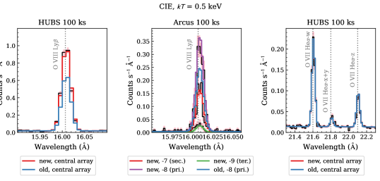
Figure 7: Simulated HUBS (left and right) and Arcus (middle) spectra in the O viii Ly$\beta$ (left and middle) and O vii triplet neighbourhood. Simulated data are shown in black and the $1\sigma$ statistical uncertainties in pink. Model spectra using the new atomic data presented in this work are shown in dashed lines, while those using the atomic data from SPEX v3.06.01 are in solid blue lines. Due to geometry overlapping for Arcus, the O viii Ly$\beta$ line comes from the primary spectral order (the $-8$th order, purple) as well as two neighboring spectral orders ($-7$th and $-9$th). See text for the detailed simulation setup (Sect. 6.4).

7 Summary

We have presented systematic radiation damped $R$-matrix intermediate-coupling frame transformation calculations of electron-impact excitation data of H- and He-like ions with atomic number $Z=6-30$. For each ion, fine-structure energy levels up to $n=6$ (36 levels for H-like ions and 71 levels for He-like ions) were included in the target configuration interaction and close-coupling collision expansion. Level-resolved effective collision strengths were obtained among these levels over four orders of magnitude in temperature. When compared with existing $R$-matrix or distorted wave data in the atomic databases and literature, generally speaking, relatively good agreements can be found near the peak temperatures of charge state distribution under collisional ionized equilibrium conditions. The new data calculated here are relevant for current and future high-resolution X-ray spectrometers such as the upcoming XRISM in 2023, Athena/X-IFU, HUBS, Arcus, and so on around 2030s.

Appendix A Level energies and $A$-values of H- and He-like key diagnostic lines

Accurate level energies are essential to obtain the correct rest frame line energy (or wavelength). The level energies of the upper levels of the key diagnostics lines in Table 1 agree well among the three databases with only a few exceptions (Tables 4 and  5). For H-like ones, the largest difference comes from the level energy of Ar xviii ${\rm 2p}~{}(^{2}P_{1/2})$ in CHIANTI (taken from Phillips et al., 2003), which is lower than AtomDB/SPEX by 0.4 eV. For He-like ones, the largest difference comes from the level energy of Mg xi ${\rm 1s~{}3p~{}^{1}P_{1}}$ in SPEX, which is lower by 0.7 eV than AtomDB/CHIANTI. This can be comparable to the energy gain correction of the instrument, as shown in the analysis of the Hitomi/SXS spectrum of the Perseus galaxy cluster (Hitomi Collaboration et al., 2018a). The derived bulk velocity of the intracluster media differs by $6~{}{\rm km~{}s^{-1}}$ between SPEX v3.03 and AtomDB v3.0.8, while the energy gain correction of the instrument is $14~{}{\rm km~{}s^{-1}}$.

As discussed in Sect. 6, the AS-RM energy levels are less accurate than those that can be obtained from AUTOSTRUCTURE without the restrictions imposed by their use by the Breit–Pauli $R$-matrix code. The latter is denoted as AS-REL. The AS-REL energy levels are also shown in Tables 4 and 5. For H-like ions, the inclusion by AUTOSTRUCTURE of the quantum electrodynamic (QED) effects (vacuum polarization and electron self-energy) reduce the inaccuracy from $\lesssim 0.05$ % to $\lesssim 0.001$ % when compared with the three atomic databases. For He-like ions: at low-charge the two-body Coulomb interaction is the main source of uncertainty ($\lesssim 0.23$ % when compared with the three atomic databases); while at high-charge relativistic effects are the main source and the inclusion as well by AUTOSTRUCTURE of the two-body relativistic interactions reduces the overall inaccuracy (from $\lesssim 0.15$ % to $\lesssim 0.03$ % for Ni XXVII when compared with the three atomic databases).

As shown in Table 6, for the $np~{}^{2}P_{3/2,1/2},~{}n=2-5$ energy levels in H-like ions, the $A$-values in AtomDB, CHIANTI, and SPEX agree well ($\lesssim 5$%) for the resonance lines. Larger deviations (up to 40%) can be found for energy levels in He-like ions (Table 7), especially the upper levels of some intercombination lines and forbidden lines.

The A-values shown in Tables  6 and 7 can differ by up to $\sim 40$ %, depending on which databases are compared. For instance, the A-value of the C v He$\alpha$-y line differs between AS-RM and SPEX by $\sim 40$ %, while the AS-RM and AtomDB values are identical. The A-value for this transition in CHIANTI is $\sim 27$ % larger than the AS-RM/AtomDB ones. We are limited to using non-relativistic orbitals (by our scattering calculation) but the perturbative one-body relativistic operators (mass-velocity and Darwin) become increasingly large as the ion charge increases and imbalance the level mixing which in turn leads to the relatively low accuracy for the AS-RM He$\gamma$-w, He$\delta$-w transition rates of high-$Z$ elements. Using (kappa-averaged) relativistic orbitals in AUTOSTRUCTURE eliminates the perturbative imbalance. This can be seen most clearly for H-like ions (where the databases agree well.) The AS-RM Ni xxviii Ly$\delta$ A-values in Table 6 are $\sim$20% smaller than the database ones. AUTOSTRUCTURE calculations using relativistic orbitals reduce the difference to a few percent, depending on the database. These transitions are shown in the last columns of Tables 6 and 7. The corresponding Ni xxvii He$\gamma$-w, He$\delta$-w transition rates now agree with CHIANTI to within 3%. Both the AS-RM and AS-REL data sets (in the adf04 format) are available in the Zenodo package.

Table 4: Energy levels (in eV) of H-like ions in SPEX v3.06.01, AtomDB v3.0.9, and CHIANTI database v10.0.1. The numbers in the parentheses are the differences (in eV) with respect to SPEX of the other two databases. The penultimate column shows the results of the present AUTOSTRUCTURE calculations which were used for the R-matrix calculations (AS-RM). The last column shows the results of AUTOSTRUCTURE calculations including relativistic effects (AS-REL) that are necessarily omitted by AS-RM. See the discussion in Sect. 6 and Appendix A.

Ion	Level	SPEX	AtomDB	CHIANTI	AS-RM	AS-REL
C vi	${\rm 2p~{}^{2}P_{1/2}}$	367.5	367.5 (-0.0)	367.5 (-0.0)	367.5	367.5
C vi	${\rm 2p~{}^{2}P_{3/2}}$	367.5	367.5 (-0.0)	367.5 (-0.0)	367.6	367.6
C vi	${\rm 3p~{}^{2}P_{1/2}}$	435.5	435.5 (-0.0)	435.5 (-0.0)	435.6	435.6
C vi	${\rm 3p~{}^{2}P_{3/2}}$	435.6	435.6 (-0.0)	435.6 (-0.0)	435.6	435.6
C vi	${\rm 4p~{}^{2}P_{1/2}}$	459.4	459.4 (-0.0)	459.4 (-0.0)	459.4	459.4
C vi	${\rm 4p~{}^{2}P_{3/2}}$	459.4	459.4 (-0.0)	459.4 (-0.0)	459.4	459.4
C vi	${\rm 5p~{}^{2}P_{1/2}}$	470.4	470.4 (-0.0)	470.4 (-0.0)	470.4	470.4
C vi	${\rm 5p~{}^{2}P_{3/2}}$	470.4	470.4 (-0.0)	470.4 (-0.0)	470.4	470.4
N vii	${\rm 2p~{}^{2}P_{1/2}}$	500.2	500.2 (-0.0)	500.2 (-0.0)	500.3	500.3
N vii	${\rm 2p~{}^{2}P_{3/2}}$	500.4	500.4 (-0.0)	500.4 (-0.0)	500.4	500.4
N vii	${\rm 3p~{}^{2}P_{1/2}}$	592.9	592.9 (-0.0)	592.9 (-0.0)	593.0	593.0
N vii	${\rm 3p~{}^{2}P_{3/2}}$	593.0	593.0 (-0.0)	593.0 (-0.0)	593.0	593.0
N vii	${\rm 4p~{}^{2}P_{1/2}}$	625.4	625.4 (-0.0)	625.4 (-0.0)	625.4	625.4
N vii	${\rm 4p~{}^{2}P_{3/2}}$	625.4	625.4 (-0.0)	625.4 (-0.0)	625.4	625.4
N vii	${\rm 5p~{}^{2}P_{1/2}}$	640.4	640.4 (-0.0)	640.4 (-0.0)	640.4	640.4
N vii	${\rm 5p~{}^{2}P_{3/2}}$	640.4	640.4 (-0.0)	640.4 (-0.0)	640.4	640.4
O viii	${\rm 2p~{}^{2}P_{1/2}}$	653.5	653.5 (-0.0)	653.5 (-0.0)	653.6	653.5
O viii	${\rm 2p~{}^{2}P_{3/2}}$	653.7	653.7 (-0.0)	653.7 (-0.0)	653.8	653.7
O viii	${\rm 3p~{}^{2}P_{1/2}}$	774.6	774.6 (-0.0)	774.6 (-0.0)	774.7	774.6
O viii	${\rm 3p~{}^{2}P_{3/2}}$	774.6	774.6 (-0.0)	774.6 (-0.0)	774.7	774.7
O viii	${\rm 4p~{}^{2}P_{1/2}}$	817.0	817.0 (-0.0)	817.0 (-0.0)	817.0	817.0
O viii	${\rm 4p~{}^{2}P_{3/2}}$	817.0	817.0 (-0.0)	817.0 (-0.0)	817.1	817.0
O viii	${\rm 5p~{}^{2}P_{1/2}}$	836.6	836.6 (-0.0)	836.6 (-0.0)	836.7	836.6
O viii	${\rm 5p~{}^{2}P_{3/2}}$	836.6	836.6 (-0.0)	836.6 (-0.0)	836.7	836.6
Ne x	${\rm 2p~{}^{2}P_{1/2}}$	1021.4	1021.5 (+0.1)	1021.5 (+0.1)	1021.7	1021.5
Ne x	${\rm 2p~{}^{2}P_{3/2}}$	1021.9	1022.0 (+0.1)	1022.0 (+0.1)	1022.1	1022.0
Ne x	${\rm 3p~{}^{2}P_{1/2}}$	1210.8	1210.8 (-0.0)	1210.8 (-0.0)	1211.0	1210.9
Ne x	${\rm 3p~{}^{2}P_{3/2}}$	1210.9	1211.0 (+0.1)	1211.0 (+0.1)	1211.1	1211.0
Ne x	${\rm 4p~{}^{2}P_{1/2}}$	1277.0	1277.1 (+0.1)	1277.1 (+0.1)	1277.3	1277.1
Ne x	${\rm 4p~{}^{2}P_{3/2}}$	1277.1	1277.1 (+0.1)	1277.1 (+0.1)	1277.3	1277.2
Ne x	${\rm 5p~{}^{2}P_{1/2}}$	1307.7	1307.7 (+0.1)	1307.7 (+0.1)	1307.9	1307.8
Ne x	${\rm 5p~{}^{2}P_{3/2}}$	1307.7	1307.8 (+0.1)	1307.8 (+0.1)	1307.9	1307.8
Na xi	${\rm 2p~{}^{2}P_{1/2}}$	1236.3	1236.3 (-0.0)	1236.3 (-0.0)	1236.5	1236.3
Na xi	${\rm 2p~{}^{2}P_{3/2}}$	1237.0	1237.0 (-0.0)	1237.0 (-0.0)	1237.2	1237.0
Na xi	${\rm 3p~{}^{2}P_{1/2}}$	1465.5	1465.5 (-0.0)	1465.5 (-0.0)	1465.7	1465.5
Na xi	${\rm 3p~{}^{2}P_{3/2}}$	1465.7	1465.7 (-0.0)	1465.7 (-0.0)	1465.9	1465.7
Na xi	${\rm 4p~{}^{2}P_{1/2}}$	1545.7	1545.7 (-0.0)	1545.7 (-0.0)	1545.9	1545.7
Na xi	${\rm 4p~{}^{2}P_{3/2}}$	1545.8	1545.8 (-0.0)	1545.8 (-0.0)	1546.0	1545.8
Na xi	${\rm 5p~{}^{2}P_{1/2}}$	1582.8	1582.8 (-0.0)	1582.8 (-0.0)	1583.0	1582.8
Na xi	${\rm 5p~{}^{2}P_{3/2}}$	1582.8	1582.8 (-0.0)	1582.8 (-0.0)	1583.1	1582.9
Mg xii	${\rm 2p~{}^{2}P_{1/2}}$	1471.7	1471.7 (+0.0)	1471.7 (+0.0)	1472.0	1471.7
Mg xii	${\rm 2p~{}^{2}P_{3/2}}$	1472.6	1472.6 (+0.0)	1472.6 (+0.0)	1472.9	1472.7
Mg xii	${\rm 3p~{}^{2}P_{1/2}}$	1744.6	1744.6 (+0.0)	1744.6 (+0.0)	1744.9	1744.6
Mg xii	${\rm 3p~{}^{2}P_{3/2}}$	1744.8	1744.8 (+0.0)	1744.8 (+0.0)	1745.2	1744.9
Mg xii	${\rm 4p~{}^{2}P_{1/2}}$	1840.0	1840.0 (+0.0)	1840.0 (+0.0)	1840.3	1840.1
Mg xii	${\rm 4p~{}^{2}P_{3/2}}$	1840.1	1840.1 (+0.0)	1840.1 (+0.0)	1840.5	1840.2
Mg xii	${\rm 5p~{}^{2}P_{1/2}}$	1884.2	1884.2 (+0.0)	1884.2 (+0.0)	1884.5	1884.2
Mg xii	${\rm 5p~{}^{2}P_{3/2}}$	1884.3	1884.3 (+0.0)	1884.3 (+0.0)	1884.6	1884.3
Al xiii	${\rm 2p~{}^{2}P_{1/2}}$	1727.7	1727.7 (+0.0)	1727.7 (+0.0)	1728.1	1727.7
Al xiii	${\rm 2p~{}^{2}P_{3/2}}$	1729.0	1729.0 (+0.0)	1729.0 (+0.0)	1729.4	1729.0
Al xiii	${\rm 3p~{}^{2}P_{1/2}}$	2048.1	2048.1 (+0.0)	2048.1 (+0.0)	2048.5	2048.1
Al xiii	${\rm 3p~{}^{2}P_{3/2}}$	2048.5	2048.5 (+0.0)	2048.5 (+0.0)	2048.9	2048.5
Al xiii	${\rm 4p~{}^{2}P_{1/2}}$	2160.2	2160.2 (+0.0)	2160.2 (+0.0)	2160.6	2160.2
Al xiii	${\rm 4p~{}^{2}P_{3/2}}$	2160.3	2160.3 (+0.0)	2160.3 (+0.0)	2160.7	2160.4
Al xiii	${\rm 5p~{}^{2}P_{1/2}}$	2212.0	2212.0 (+0.0)	2212.0 (+0.0)	2212.4	2212.1
Al xiii	${\rm 5p~{}^{2}P_{3/2}}$	2212.1	2212.1 (+0.0)	2212.1 (+0.0)	2212.5	2212.2
Si xiv	${\rm 2p~{}^{2}P_{1/2}}$	2004.3	2004.3 (+0.0)	2004.3 (+0.0)	2004.8	2004.4
Si xiv	${\rm 2p~{}^{2}P_{3/2}}$	2006.1	2006.1 (+0.0)	2006.1 (+0.0)	2006.6	2006.1
Si xiv	${\rm 3p~{}^{2}P_{1/2}}$	2376.1	2376.1 (+0.0)	2376.1 (+0.0)	2376.6	2376.2
Si xiv	${\rm 3p~{}^{2}P_{3/2}}$	2376.6	2376.6 (+0.0)	2376.6 (+0.0)	2377.1	2376.7
Si xiv	${\rm 4p~{}^{2}P_{1/2}}$	2506.2	2506.2 (+0.0)	2506.2 (+0.0)	2506.7	2506.2
Si xiv	${\rm 4p~{}^{2}P_{3/2}}$	2506.4	2506.4 (+0.0)	2506.4 (+0.0)	2506.9	2506.4
Si xiv	${\rm 5p~{}^{2}P_{1/2}}$	2566.3	2566.3 (+0.0)	2566.3 (+0.0)	2566.8	2566.4
Si xiv	${\rm 5p~{}^{2}P_{3/2}}$	2566.4	2566.4 (+0.0)	2566.4 (+0.0)	2566.9	2566.5
P xv	${\rm 2p~{}^{2}P_{1/2}}$	2301.6	2301.6 (+0.0)	2301.6 (+0.0)	2302.3	2301.7
P xv	${\rm 2p~{}^{2}P_{3/2}}$	2304.0	2304.0 (+0.0)	2304.0 (+0.0)	2304.6	2304.0
P xv	${\rm 3p~{}^{2}P_{1/2}}$	2728.7	2728.7 (+0.0)	2728.7 (+0.0)	2729.3	2728.7
P xv	${\rm 3p~{}^{2}P_{3/2}}$	2729.4	2729.4 (+0.0)	2729.4 (+0.0)	2730.0	2729.4
P xv	${\rm 4p~{}^{2}P_{1/2}}$	2878.0	2878.0 (+0.0)	2878.0 (+0.0)	2878.7	2878.1
P xv	${\rm 4p~{}^{2}P_{3/2}}$	2878.3	2878.3 (+0.0)	2878.3 (+0.0)	2879.0	2878.4
P xv	${\rm 5p~{}^{2}P_{1/2}}$	2947.1	2947.1 (+0.0)	2947.1 (+0.0)	2947.8	2947.2
P xv	${\rm 5p~{}^{2}P_{3/2}}$	2947.3	2947.3 (+0.0)	2947.3 (+0.0)	2947.9	2947.3
S xvi	${\rm 2p~{}^{2}P_{1/2}}$	2619.7	2619.7 (+0.0)	2619.7 (+0.0)	2620.5	2619.7
S xvi	${\rm 2p~{}^{2}P_{3/2}}$	2622.7	2622.7 (+0.0)	2622.7 (+0.0)	2623.4	2622.7
S xvi	${\rm 3p~{}^{2}P_{1/2}}$	3105.9	3105.9 (+0.0)	3105.9 (+0.0)	3106.6	3105.9
S xvi	${\rm 3p~{}^{2}P_{3/2}}$	3106.7	3106.7 (+0.0)	3106.7 (+0.0)	3107.5	3106.8
S xvi	${\rm 4p~{}^{2}P_{1/2}}$	3275.9	3275.9 (+0.0)	3275.9 (+0.0)	3276.7	3275.9
S xvi	${\rm 4p~{}^{2}P_{3/2}}$	3276.3	3276.3 (+0.0)	3276.3 (+0.0)	3277.0	3276.3
S xvi	${\rm 5p~{}^{2}P_{1/2}}$	3354.5	3354.5 (+0.0)	3354.5 (+0.0)	3355.3	3354.6
S xvi	${\rm 5p~{}^{2}P_{3/2}}$	3354.7	3354.7 (+0.0)	3354.7 (+0.0)	3355.5	3354.8
Cl xvii	${\rm 2p~{}^{2}P_{1/2}}$	2958.5	2958.5 (+0.0)	2958.5 (-0.0)	2959.5	2958.6
Cl xvii	${\rm 2p~{}^{2}P_{3/2}}$	2962.3	2962.4 (+0.0)	2962.3 (-0.0)	2963.3	2962.4
Cl xvii	${\rm 3p~{}^{2}P_{1/2}}$	3507.7	3507.7 (+0.0)	3507.7 (-0.0)	3508.6	3507.8
Cl xvii	${\rm 3p~{}^{2}P_{3/2}}$	3508.8	3508.8 (+0.0)	3508.8 (-0.0)	3509.8	3508.9
Cl xvii	${\rm 4p~{}^{2}P_{1/2}}$	3699.8	3699.8 (+0.0)	3699.8 (-0.0)	3700.7	3699.8
Cl xvii	${\rm 4p~{}^{2}P_{3/2}}$	3700.2	3700.2 (+0.0)	3700.2 (-0.0)	3701.2	3700.3
Cl xvii	${\rm 5p~{}^{2}P_{1/2}}$	3788.6	3788.6 (+0.0)	3788.6 (-0.0)	3789.5	3788.7
Cl xvii	${\rm 5p~{}^{2}P_{3/2}}$	3788.8	3788.8 (+0.0)	3788.8 (-0.0)	3789.8	3788.9
Ar xviii	${\rm 2p~{}^{2}P_{1/2}}$	3318.2	3318.2 (+0.0)	3317.7 (-0.4)	3319.3	3318.2
Ar xviii	${\rm 2p~{}^{2}P_{3/2}}$	3323.0	3323.0 (+0.0)	3323.1 (+0.1)	3324.1	3323.0
Ar xviii	${\rm 3p~{}^{2}P_{1/2}}$	3934.3	3934.3 (+0.0)	3934.3 (+0.0)	3935.4	3934.3
Ar xviii	${\rm 3p~{}^{2}P_{3/2}}$	3935.7	3935.7 (+0.0)	3935.7 (+0.0)	3936.8	3935.8
Ar xviii	${\rm 4p~{}^{2}P_{1/2}}$	4149.7	4149.7 (+0.0)	4149.7 (+0.0)	4150.8	4149.8
Ar xviii	${\rm 4p~{}^{2}P_{3/2}}$	4150.3	4150.3 (+0.0)	4150.3 (+0.0)	4151.4	4150.4
Ar xviii	${\rm 5p~{}^{2}P_{1/2}}$	4249.4	4249.4 (+0.0)	4249.4 (+0.0)	4250.5	4249.4
Ar xviii	${\rm 5p~{}^{2}P_{3/2}}$	4249.7	4249.7 (+0.0)	4249.7 (+0.0)	4250.8	4249.7
K xix	${\rm 2p~{}^{2}P_{1/2}}$	3698.7	3698.7 (+0.0)	3698.7 (+0.0)	3700.0	3698.7
K xix	${\rm 2p~{}^{2}P_{3/2}}$	3704.7	3704.7 (+0.0)	3704.7 (+0.0)	3705.9	3704.7
K xix	${\rm 3p~{}^{2}P_{1/2}}$	4385.7	4385.7 (+0.0)	4385.7 (+0.0)	4387.0	4385.7
K xix	${\rm 3p~{}^{2}P_{3/2}}$	4387.4	4387.4 (+0.0)	4387.4 (+0.0)	4388.7	4387.5
K xix	${\rm 4p~{}^{2}P_{1/2}}$	4625.8	4625.9 (+0.0)	4625.9 (+0.0)	4627.2	4625.9
K xix	${\rm 4p~{}^{2}P_{3/2}}$	4626.6	4626.6 (+0.0)	4626.6 (+0.0)	4627.9	4626.7
K xix	${\rm 5p~{}^{2}P_{1/2}}$	4736.9	4736.9 (+0.0)	4736.9 (+0.0)	4738.2	4737.0
K xix	${\rm 5p~{}^{2}P_{3/2}}$	4737.3	4737.3 (+0.0)	4737.3 (+0.0)	4738.6	4737.4
Ca xx	${\rm 2p~{}^{2}P_{1/2}}$	4100.1	4100.1 (+0.0)	4100.1 (+0.0)	4101.7	4100.2
Ca xx	${\rm 2p~{}^{2}P_{3/2}}$	4107.5	4107.5 (+0.0)	4107.5 (+0.0)	4109.0	4107.6
Ca xx	${\rm 3p~{}^{2}P_{1/2}}$	4861.9	4861.9 (+0.0)	4861.9 (+0.0)	4863.5	4862.0
Ca xx	${\rm 3p~{}^{2}P_{3/2}}$	4864.1	4864.1 (+0.0)	4864.1 (+0.0)	4865.6	4864.2
Ca xx	${\rm 4p~{}^{2}P_{1/2}}$	5128.2	5128.2 (+0.0)	5128.2 (+0.0)	5129.8	5128.3
Ca xx	${\rm 4p~{}^{2}P_{3/2}}$	5129.1	5129.2 (+0.0)	5129.2 (+0.0)	5130.7	5129.2
Ca xx	${\rm 5p~{}^{2}P_{1/2}}$	5251.4	5251.4 (+0.0)	5251.4 (+0.0)	5252.9	5251.5
Ca xx	${\rm 5p~{}^{2}P_{3/2}}$	5251.8	5251.8 (+0.0)	5251.8 (+0.0)	5253.3	5251.9
Cr xxiv	${\rm 2p~{}^{2}P_{1/2}}$	5916.4	5916.5 (+0.1)	– –	5919.1	5916.5
Cr xxiv	${\rm 2p~{}^{2}P_{3/2}}$	5931.8	5931.9 (+0.1)	– –	5934.3	5931.9
Cr xxiv	${\rm 3p~{}^{2}P_{1/2}}$	7017.2	7017.3 (+0.1)	– –	7019.9	7017.3
Cr xxiv	${\rm 3p~{}^{2}P_{3/2}}$	7021.7	7021.8 (+0.1)	– –	7024.3	7021.9
Cr xxiv	${\rm 4p~{}^{2}P_{1/2}}$	7401.8	7401.9 (+0.1)	– –	7404.5	7402.0
Cr xxiv	${\rm 4p~{}^{2}P_{3/2}}$	7403.8	7403.8 (+0.1)	– –	7406.3	7403.9
Cr xxiv	${\rm 5p~{}^{2}P_{1/2}}$	7579.6	7579.7 (+0.1)	– –	7582.2	7579.8
Cr xxiv	${\rm 5p~{}^{2}P_{3/2}}$	7580.6	7580.7 (+0.1)	– –	7583.1	7580.7
Mn xxv	${\rm 2p~{}^{2}P_{1/2}}$	6423.5	6423.6 (+0.1)	– –	6426.5	6423.5
Mn xxv	${\rm 2p~{}^{2}P_{3/2}}$	6441.6	6441.7 (+0.1)	– –	6444.4	6441.7
Mn xxv	${\rm 3p~{}^{2}P_{1/2}}$	7619.1	7619.1 (+0.1)	– –	7622.0	7619.2
Mn xxv	${\rm 3p~{}^{2}P_{3/2}}$	7624.4	7624.5 (+0.1)	– –	7627.2	7624.6
Mn xxv	${\rm 4p~{}^{2}P_{1/2}}$	8036.8	8036.8 (+0.1)	– –	8039.7	8036.9
Mn xxv	${\rm 4p~{}^{2}P_{3/2}}$	8039.0	8039.1 (+0.1)	– –	8041.9	8039.2
Mn xxv	${\rm 5p~{}^{2}P_{1/2}}$	8229.8	8229.9 (+0.1)	– –	8232.7	8229.9
Mn xxv	${\rm 5p~{}^{2}P_{3/2}}$	8230.9	8231.0 (+0.1)	– –	8233.8	8231.1
Fe xxvi	${\rm 2p~{}^{2}P_{1/2}}$	6951.9	6952.0 (+0.1)	6952.0 (+0.1)	6955.2	6951.9
Fe xxvi	${\rm 2p~{}^{2}P_{3/2}}$	6973.1	6973.2 (+0.1)	6973.2 (+0.1)	6976.2	6973.2
Fe xxvi	${\rm 3p~{}^{2}P_{1/2}}$	8246.3	8246.4 (+0.1)	8246.4 (+0.1)	8249.6	8246.5
Fe xxvi	${\rm 3p~{}^{2}P_{3/2}}$	8252.6	8252.7 (+0.1)	8252.7 (+0.1)	8255.7	8252.8
Fe xxvi	${\rm 4p~{}^{2}P_{1/2}}$	8698.5	8698.6 (+0.1)	8698.6 (+0.1)	8701.7	8698.7
Fe xxvi	${\rm 4p~{}^{2}P_{3/2}}$	8701.1	8701.2 (+0.1)	8701.2 (+0.1)	8704.3	8701.3
Fe xxvi	${\rm 5p~{}^{2}P_{1/2}}$	8907.4	8907.5 (+0.1)	8907.5 (+0.1)	8910.6	8907.6
Fe xxvi	${\rm 5p~{}^{2}P_{3/2}}$	8908.8	8908.9 (+0.1)	8908.9 (+0.1)	8911.9	8908.9
Ni xxviii	${\rm 2p~{}^{2}P_{1/2}}$	8073.0	8073.1 (+0.1)	8073.1 (+0.1)	8077.1	8073.0
Ni xxviii	${\rm 2p~{}^{2}P_{3/2}}$	8101.6	8101.7 (+0.1)	8101.7 (+0.1)	8105.3	8101.8
Ni xxviii	${\rm 3p~{}^{2}P_{1/2}}$	9577.4	9577.6 (+0.1)	9577.6 (+0.1)	9581.5	9577.6
Ni xxviii	${\rm 3p~{}^{2}P_{3/2}}$	9585.9	9586.1 (+0.1)	9586.1 (+0.1)	9589.6	9586.1
Ni xxviii	${\rm 4p~{}^{2}P_{1/2}}$	10102.8	10103.0 (+0.1)	10103.0 (+0.1)	10106.7	10103.0
Ni xxviii	${\rm 4p~{}^{2}P_{3/2}}$	10106.4	10106.5 (+0.1)	10106.5 (+0.1)	10110.1	10106.6
Ni xxviii	${\rm 5p~{}^{2}P_{1/2}}$	10345.5	10345.6 (+0.1)	10345.6 (+0.1)	10349.4	10345.7
Ni xxviii	${\rm 5p~{}^{2}P_{3/2}}$	10347.3	10347.5 (+0.1)	10347.5 (+0.1)	10351.1	10347.6

Table 5: Energy levels (in eV) of He-like ions in SPEX v3.06.01, AtomDB v3.0.9, and CHIANTI database v10.0.1. The numbers in the parentheses are the differences (in eV) with respect to SPEX of the other two databases. The penultimate column shows the results of the present AUTOSTRUCTURE calculations which were used for the R-matrix calculations (AS-RM). The last column shows the results of AUTOSTRUCTURE calculations including relativistic effects (AS-REL) that are necessarily omitted by AS-RM. See the discussion in Sect. 6 and Appendix A.

Ion	Level	SPEX	AtomDB	CHIANTI	AS-RM	AS-REL
C v	${\rm 1s~{}2p~{}^{1}P_{1}}$	307.9	307.9 (+0.0)	307.9 (+0.0)	308.6	308.5
C v	${\rm 1s~{}2p~{}^{3}P_{2}}$	304.4	304.4 (+0.0)	304.4 (+0.0)	304.5	304.5
C v	${\rm 1s~{}2p~{}^{3}P_{1}}$	304.4	304.4 (+0.0)	304.4 (+0.0)	304.5	304.4
C v	${\rm 1s~{}2s~{}^{3}S_{1}}$	299.0	299.0 (+0.0)	299.0 (+0.0)	299.0	298.9
C v	${\rm 1s~{}3p~{}^{1}P_{1}}$	354.5	354.5 (-0.0)	354.5 (-0.0)	354.9	354.8
C v	${\rm 1s~{}4p~{}^{1}P_{1}}$	370.9	370.9 (-0.0)	370.9 (-0.0)	371.3	371.2
C v	${\rm 1s~{}5p~{}^{1}P_{1}}$	378.5	378.5 (-0.0)	378.5 (-0.0)	378.9	378.8
N vi	${\rm 1s~{}2p~{}^{1}P_{1}}$	430.7	430.7 (-0.0)	430.7 (+0.0)	431.4	431.3
N vi	${\rm 1s~{}2p~{}^{3}P_{2}}$	426.3	426.3 (-0.0)	426.3 (-0.0)	426.5	426.3
N vi	${\rm 1s~{}2p~{}^{3}P_{1}}$	426.3	426.3 (-0.0)	426.3 (-0.0)	426.4	426.3
N vi	${\rm 1s~{}2s~{}^{3}S_{1}}$	419.8	419.8 (-0.0)	419.8 (-0.0)	419.9	419.8
N vi	${\rm 1s~{}3p~{}^{1}P_{1}}$	498.0	498.0 (-0.0)	498.0 (-0.0)	498.4	498.3
N vi	${\rm 1s~{}4p~{}^{1}P_{1}}$	521.6	521.6 (-0.0)	521.6 (-0.0)	522.0	521.8
N vi	${\rm 1s~{}5p~{}^{1}P_{1}}$	532.6	532.6 (+0.0)	532.6 (+0.0)	532.9	532.8
O vii	${\rm 1s~{}2p~{}^{1}P_{1}}$	573.9	573.9 (-0.0)	574.0 (+0.0)	574.8	574.6
O vii	${\rm 1s~{}2p~{}^{3}P_{2}}$	568.6	568.6 (-0.0)	568.7 (+0.1)	568.9	568.7
O vii	${\rm 1s~{}2p~{}^{3}P_{1}}$	568.6	568.6 (-0.0)	568.6 (+0.1)	568.9	568.7
O vii	${\rm 1s~{}2s~{}^{3}S_{1}}$	561.0	561.0 (-0.0)	561.1 (+0.1)	561.2	561.0
O vii	${\rm 1s~{}3p~{}^{1}P_{1}}$	665.6	665.6 (-0.0)	665.6 (-0.0)	666.1	665.9
O vii	${\rm 1s~{}4p~{}^{1}P_{1}}$	697.8	697.8 (-0.0)	697.8 (-0.0)	698.3	698.1
O vii	${\rm 1s~{}5p~{}^{1}P_{1}}$	712.7	712.7 (-0.0)	712.7 (-0.0)	713.2	713.0
Ne ix	${\rm 1s~{}2p~{}^{1}P_{1}}$	922.0	922.0 (-0.0)	922.0 (-0.0)	923.1	922.7
Ne ix	${\rm 1s~{}2p~{}^{3}P_{2}}$	915.0	915.0 (-0.0)	915.0 (-0.0)	915.5	914.9
Ne ix	${\rm 1s~{}2p~{}^{3}P_{1}}$	914.8	914.8 (-0.0)	914.8 (-0.0)	915.2	914.8
Ne ix	${\rm 1s~{}2s~{}^{3}S_{1}}$	905.1	905.1 (-0.0)	905.1 (-0.0)	905.5	905.0
Ne ix	${\rm 1s~{}3p~{}^{1}P_{1}}$	1073.8	1073.8 (-0.0)	1073.8 (-0.0)	1074.6	1074.1
Ne ix	${\rm 1s~{}4p~{}^{1}P_{1}}$	1127.1	1127.1 (-0.0)	1127.1 (-0.0)	1127.8	1127.3
Ne ix	${\rm 1s~{}5p~{}^{1}P_{1}}$	1151.8	1151.8 (-0.0)	1151.8 (-0.0)	1152.5	1152.0
Na x	${\rm 1s~{}2p~{}^{1}P_{1}}$	1126.9	1126.9 (+0.0)	1126.9 (-0.0)	1128.1	1127.5
Na x	${\rm 1s~{}2p~{}^{3}P_{2}}$	1119.0	1119.0 (+0.0)	1119.0 (+0.0)	1119.6	1118.9
Na x	${\rm 1s~{}2p~{}^{3}P_{1}}$	1118.7	1118.7 (+0.0)	1118.7 (-0.0)	1119.3	1118.6
Na x	${\rm 1s~{}2s~{}^{3}S_{1}}$	1107.8	1107.8 (+0.0)	1107.8 (-0.0)	1108.4	1107.8
Na x	${\rm 1s~{}3p~{}^{1}P_{1}}$	1314.4	1314.4 (-0.0)	1314.4 (-0.0)	1315.3	1314.7
Na x	${\rm 1s~{}4p~{}^{1}P_{1}}$	1380.2	1380.2 (+0.0)	1380.2 (+0.0)	1381.1	1380.5
Na x	${\rm 1s~{}5p~{}^{1}P_{1}}$	1410.8	1410.8 (-0.0)	1410.8 (-0.0)	1411.6	1411.0
Mg xi	${\rm 1s~{}2p~{}^{1}P_{1}}$	1352.2	1352.2 (+0.0)	1352.2 (+0.0)	1353.8	1353.0
Mg xi	${\rm 1s~{}2p~{}^{3}P_{2}}$	1343.5	1343.5 (+0.0)	1343.5 (+0.0)	1344.4	1343.4
Mg xi	${\rm 1s~{}2p~{}^{3}P_{1}}$	1343.1	1343.1 (+0.0)	1343.1 (+0.0)	1343.9	1343.0
Mg xi	${\rm 1s~{}2s~{}^{3}S_{1}}$	1331.1	1331.1 (+0.0)	1331.1 (+0.0)	1331.9	1331.0
Mg xi	${\rm 1s~{}3p~{}^{1}P_{1}}$	1580.0	1579.3 (-0.7)	1579.3 (-0.7)	1580.5	1579.6
Mg xi	${\rm 1s~{}4p~{}^{1}P_{1}}$	1659.1	1659.1 (-0.0)	1659.1 (-0.0)	1660.2	1659.3
Mg xi	${\rm 1s~{}5p~{}^{1}P_{1}}$	1696.0	1696.0 (+0.0)	1696.0 (+0.0)	1697.1	1696.3
Al xii	${\rm 1s~{}2p~{}^{1}P_{1}}$	1598.3	1598.3 (-0.1)	1598.3 (-0.0)	1600.1	1599.1
Al xii	${\rm 1s~{}2p~{}^{3}P_{2}}$	1588.8	1588.8 (-0.0)	1588.8 (-0.0)	1589.9	1588.6
Al xii	${\rm 1s~{}2p~{}^{3}P_{1}}$	1588.2	1588.1 (-0.0)	1588.1 (-0.0)	1589.1	1588.0
Al xii	${\rm 1s~{}2s~{}^{3}S_{1}}$	1575.0	1575.0 (-0.1)	1575.0 (-0.0)	1576.0	1574.9
Al xii	${\rm 1s~{}3p~{}^{1}P_{1}}$	1868.8	1868.7 (-0.0)	1868.7 (-0.0)	1870.2	1869.0
Al xii	${\rm 1s~{}4p~{}^{1}P_{1}}$	1963.7	1963.7 (-0.0)	1963.7 (-0.0)	1965.1	1963.9
Al xii	${\rm 1s~{}5p~{}^{1}P_{1}}$	2007.7	2007.7 (-0.0)	2007.7 (-0.0)	2009.0	2007.9
Si xiii	${\rm 1s~{}2p~{}^{1}P_{1}}$	1865.0	1865.0 (-0.0)	1865.0 (+0.0)	1867.1	1865.8
Si xiii	${\rm 1s~{}2p~{}^{3}P_{2}}$	1854.6	1854.6 (+0.0)	1854.7 (+0.0)	1856.1	1854.5
Si xiii	${\rm 1s~{}2p~{}^{3}P_{1}}$	1853.8	1853.8 (-0.0)	1853.8 (+0.0)	1855.1	1853.6
Si xiii	${\rm 1s~{}2s~{}^{3}S_{1}}$	1839.4	1839.4 (-0.0)	1839.4 (+0.0)	1840.8	1839.4
Si xiii	${\rm 1s~{}3p~{}^{1}P_{1}}$	2182.5	2182.5 (-0.0)	2182.5 (-0.0)	2184.3	2182.9
Si xiii	${\rm 1s~{}4p~{}^{1}P_{1}}$	2294.0	2294.0 (+0.0)	2294.0 (+0.0)	2295.8	2294.3
Si xiii	${\rm 1s~{}5p~{}^{1}P_{1}}$	2345.7	2345.7 (+0.0)	2345.7 (+0.0)	2347.4	2346.0
P xiv	${\rm 1s~{}2p~{}^{1}P_{1}}$	2152.5	2152.4 (-0.1)	2152.4 (-0.1)	2154.9	2153.3
P xiv	${\rm 1s~{}2p~{}^{3}P_{2}}$	2141.4	2141.3 (-0.1)	2141.3 (-0.1)	2143.1	2141.1
P xiv	${\rm 1s~{}2p~{}^{3}P_{1}}$	2140.2	2140.1 (-0.1)	2140.1 (-0.1)	2141.7	2139.9
P xiv	${\rm 1s~{}2s~{}^{3}S_{1}}$	2124.7	2124.6 (-0.1)	2124.6 (-0.1)	2126.3	2124.5
P xiv	${\rm 1s~{}3p~{}^{1}P_{1}}$	2521.1	2521.0 (-0.1)	2521.0 (-0.1)	2523.1	2521.3
P xiv	${\rm 1s~{}4p~{}^{1}P_{1}}$	2650.4	2650.3 (-0.1)	2650.3 (-0.1)	2652.4	2650.6
P xiv	${\rm 1s~{}5p~{}^{1}P_{1}}$	2710.4	2710.3 (-0.1)	2710.2 (-0.1)	2712.3	2710.5
S xv	${\rm 1s~{}2p~{}^{1}P_{1}}$	2460.6	2460.6 (+0.0)	2460.6 (+0.0)	2463.5	2461.5
S xv	${\rm 1s~{}2p~{}^{3}P_{2}}$	2448.8	2448.8 (-0.0)	2448.8 (+0.0)	2450.9	2448.4
S xv	${\rm 1s~{}2p~{}^{3}P_{1}}$	2447.1	2447.1 (+0.0)	2447.0 (-0.1)	2449.1	2446.9
S xv	${\rm 1s~{}2s~{}^{3}S_{1}}$	2430.3	2430.3 (-0.0)	2430.4 (+0.0)	2432.5	2430.3
S xv	${\rm 1s~{}3p~{}^{1}P_{1}}$	2883.9	2883.9 (+0.0)	2883.9 (-0.0)	2886.5	2884.3
S xv	${\rm 1s~{}4p~{}^{1}P_{1}}$	3032.5	3032.5 (+0.0)	3032.5 (+0.0)	3035.0	3032.8
S xv	${\rm 1s~{}5p~{}^{1}P_{1}}$	3101.3	3101.3 (+0.0)	3101.3 (-0.0)	3103.8	3101.6
Cl xvi	${\rm 1s~{}2p~{}^{1}P_{1}}$	2789.8	2789.7 (-0.1)	2789.7 (-0.1)	2793.0	2790.6
Cl xvi	${\rm 1s~{}2p~{}^{3}P_{2}}$	2777.2	2777.1 (-0.1)	2777.1 (-0.1)	2779.7	2776.7
Cl xvi	${\rm 1s~{}2p~{}^{3}P_{1}}$	2775.1	2775.0 (-0.1)	2775.0 (-0.1)	2777.3	2774.6
Cl xvi	${\rm 1s~{}2s~{}^{3}S_{1}}$	2757.0	2756.9 (-0.1)	2756.9 (-0.1)	2759.4	2756.8
Cl xvi	${\rm 1s~{}3p~{}^{1}P_{1}}$	3271.7	3271.6 (-0.1)	3271.6 (-0.1)	3274.5	3271.9
Cl xvi	${\rm 1s~{}4p~{}^{1}P_{1}}$	3440.8	3440.8 (-0.0)	3440.8 (-0.0)	3443.6	3440.9
Cl xvi	${\rm 1s~{}5p~{}^{1}P_{1}}$	3519.2	3519.1 (-0.1)	3519.1 (-0.1)	3521.9	3519.2
Ar xvii	${\rm 1s~{}2p~{}^{1}P_{1}}$	3139.8	3139.6 (-0.2)	3139.6 (-0.2)	3143.5	3140.6
Ar xvii	${\rm 1s~{}2p~{}^{3}P_{2}}$	3126.5	3126.3 (-0.2)	3126.3 (-0.2)	3129.4	3125.8
Ar xvii	${\rm 1s~{}2p~{}^{3}P_{1}}$	3123.7	3123.5 (-0.2)	3123.5 (-0.2)	3126.4	3123.2
Ar xvii	${\rm 1s~{}2s~{}^{3}S_{1}}$	3104.3	3104.1 (-0.2)	3104.1 (-0.2)	3107.2	3104.1
Ar xvii	${\rm 1s~{}3p~{}^{1}P_{1}}$	3684.0	3683.8 (-0.2)	3684.0 (-0.0)	3687.4	3684.2
Ar xvii	${\rm 1s~{}4p~{}^{1}P_{1}}$	3875.0	3874.9 (-0.2)	3875.0 (-0.0)	3878.3	3875.1
Ar xvii	${\rm 1s~{}5p~{}^{1}P_{1}}$	3963.5	3963.3 (-0.2)	3963.5 (-0.0)	3966.8	3963.5
K xviii	${\rm 1s~{}2p~{}^{1}P_{1}}$	3510.4	3510.5 (+0.2)	3510.4 (-0.0)	3515.0	3511.5
K xviii	${\rm 1s~{}2p~{}^{3}P_{2}}$	3496.5	3496.5 (+0.1)	3496.5 (-0.0)	3500.2	3496.0
K xviii	${\rm 1s~{}2p~{}^{3}P_{1}}$	3493.0	3493.0 (+0.1)	3493.0 (-0.0)	3496.4	3492.5
K xviii	${\rm 1s~{}2s~{}^{3}S_{1}}$	3472.2	3472.3 (+0.1)	3472.2 (-0.0)	3475.9	3472.2
K xviii	${\rm 1s~{}3p~{}^{1}P_{1}}$	4120.9	4120.8 (-0.1)	4120.9 (-0.0)	4125.1	4121.3
K xviii	${\rm 1s~{}4p~{}^{1}P_{1}}$	4335.1	4335.1 (+0.0)	4335.1 (-0.0)	4339.2	4335.4
K xviii	${\rm 1s~{}5p~{}^{1}P_{1}}$	4434.3	4434.3 (-0.0)	4434.3 (-0.0)	4438.4	4434.6
Ca xix	${\rm 1s~{}2p~{}^{1}P_{1}}$	3902.3	3902.3 (-0.0)	3902.2 (-0.1)	3907.6	3903.5
Ca xix	${\rm 1s~{}2p~{}^{3}P_{2}}$	3887.7	3887.7 (-0.0)	3887.6 (-0.1)	3892.2	3887.2
Ca xix	${\rm 1s~{}2p~{}^{3}P_{1}}$	3883.3	3883.3 (-0.0)	3883.2 (-0.1)	3887.4	3882.8
Ca xix	${\rm 1s~{}2s~{}^{3}S_{1}}$	3861.1	3861.1 (-0.0)	3861.1 (-0.0)	3865.6	3861.2
Ca xix	${\rm 1s~{}3p~{}^{1}P_{1}}$	4582.8	4582.8 (-0.0)	4582.8 (-0.0)	4587.7	4583.3
Ca xix	${\rm 1s~{}4p~{}^{1}P_{1}}$	4821.6	4821.6 (-0.0)	4821.6 (-0.0)	4826.4	4821.9
Ca xix	${\rm 1s~{}5p~{}^{1}P_{1}}$	4932.2	4932.2 (-0.0)	4932.2 (-0.0)	4937.0	4932.5
Cr xxiii	${\rm 1s~{}2p~{}^{1}P_{1}}$	5682.1	5682.1 (+0.0)	5682.1 (+0.1)	5690.7	5683.6
Cr xxiii	${\rm 1s~{}2p~{}^{3}P_{2}}$	5665.1	5665.1 (-0.0)	5665.1 (+0.0)	5672.9	5664.1
Cr xxiii	${\rm 1s~{}2p~{}^{3}P_{1}}$	5654.8	5654.8 (-0.0)	5654.8 (-0.1)	5662.2	5654.1
Cr xxiii	${\rm 1s~{}2s~{}^{3}S_{1}}$	5626.9	5626.9 (+0.0)	5626.9 (+0.0)	5634.7	5627.0
Cr xxiii	${\rm 1s~{}3p~{}^{1}P_{1}}$	6680.8	6680.8 (-0.0)	6681.2 (+0.4)	6689.0	6681.4
Cr xxiii	${\rm 1s~{}4p~{}^{1}P_{1}}$	7031.2	7031.2 (+0.0)	7031.4 (+0.2)	7039.4	7031.6
Cr xxiii	${\rm 1s~{}5p~{}^{1}P_{1}}$	7193.4	7193.5 (+0.1)	7193.6 (+0.2)	7201.7	7193.8
Mn xxiv	${\rm 1s~{}2p~{}^{1}P_{1}}$	6180.2	6180.4 (+0.3)	– –	6190.1	6182.1
Mn xxiv	${\rm 1s~{}2p~{}^{3}P_{2}}$	6162.8	6162.9 (+0.1)	– –	6171.7	6161.8
Mn xxiv	${\rm 1s~{}2p~{}^{3}P_{1}}$	6150.7	6150.6 (-0.1)	– –	6158.9	6149.8
Mn xxiv	${\rm 1s~{}2s~{}^{3}S_{1}}$	6121.1	6121.1 (+0.1)	– –	6130.0	6121.3
Mn xxiv	${\rm 1s~{}3p~{}^{1}P_{1}}$	7268.2	7268.3 (+0.0)	– –	7277.6	7268.9
Mn xxiv	${\rm 1s~{}4p~{}^{1}P_{1}}$	7649.9	7650.0 (+0.1)	– –	7659.2	7650.4
Mn xxiv	${\rm 1s~{}5p~{}^{1}P_{1}}$	7826.6	7826.7 (+0.1)	– –	7836.0	7827.0
Fe xxv	${\rm 1s~{}2p~{}^{1}P_{1}}$	6700.4	6700.4 (-0.0)	6700.5 (+0.1)	6711.2	6702.3
Fe xxv	${\rm 1s~{}2p~{}^{3}P_{2}}$	6682.3	6682.3 (+0.0)	6682.7 (+0.4)	6692.3	6681.1
Fe xxv	${\rm 1s~{}2p~{}^{3}P_{1}}$	6667.6	6667.6 (-0.0)	6667.7 (+0.1)	6677.0	6666.7
Fe xxv	${\rm 1s~{}2s~{}^{3}S_{1}}$	6636.6	6636.6 (+0.0)	6636.6 (+0.0)	6646.6	6636.8
Fe xxv	${\rm 1s~{}3p~{}^{1}P_{1}}$	7881.1	7881.2 (+0.0)	7881.1 (-0.0)	7891.6	7881.8
Fe xxv	${\rm 1s~{}4p~{}^{1}P_{1}}$	8295.4	8295.5 (+0.1)	8295.4 (-0.0)	8305.9	8295.9
Fe xxv	${\rm 1s~{}5p~{}^{1}P_{1}}$	8487.2	8487.3 (+0.1)	8487.2 (-0.0)	8497.7	8487.7
Ni xxvii	${\rm 1s~{}2p~{}^{1}P_{1}}$	7805.1	7805.6 (+0.4)	7805.6 (+0.5)	7818.9	7807.7
Ni xxvii	${\rm 1s~{}2p~{}^{3}P_{2}}$	7786.4	7786.4 (+0.0)	7786.4 (+0.1)	7798.9	7785.0
Ni xxvii	${\rm 1s~{}2p~{}^{3}P_{1}}$	7766.0	7765.7 (-0.4)	7765.7 (-0.3)	7777.7	7764.7
Ni xxvii	${\rm 1s~{}2s~{}^{3}S_{1}}$	7731.5	7731.6 (+0.1)	7731.6 (+0.1)	7744.2	7732.0
Ni xxvii	${\rm 1s~{}3p~{}^{1}P_{1}}$	9183.6	9183.6 (+0.0)	9183.6 (-0.0)	9196.6	9184.5
Ni xxvii	${\rm 1s~{}4p~{}^{1}P_{1}}$	9667.1	9667.2 (+0.1)	9667.1 (-0.0)	9680.2	9667.8
Ni xxvii	${\rm 1s~{}5p~{}^{1}P_{1}}$	9891.0	9891.1 (+0.1)	9891.0 (-0.0)	9904.1	9891.6

Table 6: Lyman transition data of H-like ions in SPEX v3.06.01, AtomDB v3.0.9, CHIANTI database v10.0.1, and the present work (AUTOSTRUCTURE)

. The wavelengths (as in SPEX) are in units of Å and $A$-values in ${\rm s^{-1}}$. The column labelled $\Delta$ is the maximum percentage deviation ((max - min) / max $\times 100$%) amongst the three databases. The penultimate column shows the results of the present AUTOSTRUCTURE calculations which were used for the R-matrix calculations (AS-RM). The last column shows the results of AUTOSTRUCTURE calculations including relativistic effects (AS-REL) that are necessarily omitted by AS-RM. See the discussion in Sect. 6 and Appendix A. Ion ID $\lambda$ (Å) SPEX AtomDB CHIANTI $\Delta$ AS-RM AS-REL C vi Ly$\alpha_{1/2}$ 33.740 $8.12\times 10^{11}$ $8.12\times 10^{11}$ $8.12\times 10^{11}$ 0.1% $8.12\times 10^{11}$ $8.12\times 10^{11}$ C vi Ly$\alpha_{3/2}$ 33.734 $8.12\times 10^{11}$ $8.12\times 10^{11}$ $8.12\times 10^{11}$ 0.1% $8.12\times 10^{11}$ $8.12\times 10^{11}$ C vi Ly$\beta_{1/2}$ 28.466 $2.17\times 10^{11}$ $2.17\times 10^{11}$ $2.16\times 10^{11}$ 0.3% $2.16\times 10^{11}$ $2.17\times 10^{11}$ C vi Ly$\beta_{3/2}$ 28.465 $2.17\times 10^{11}$ $2.17\times 10^{11}$ $2.16\times 10^{11}$ 0.3% $2.16\times 10^{11}$ $2.17\times 10^{11}$ C vi Ly$\gamma_{1/2}$ 26.990 $8.84\times 10^{10}$ $8.83\times 10^{10}$ $8.77\times 10^{10}$ 0.8% $8.78\times 10^{10}$ $8.82\times 10^{10}$ C vi Ly$\gamma_{3/2}$ 26.990 $8.84\times 10^{10}$ $8.84\times 10^{10}$ $8.79\times 10^{10}$ 0.5% $8.80\times 10^{10}$ $8.85\times 10^{10}$ C vi Ly$\delta_{1/2}$ 26.357 $4.46\times 10^{10}$ $4.45\times 10^{10}$ $4.38\times 10^{10}$ 1.7% $4.41\times 10^{10}$ $4.45\times 10^{10}$ C vi Ly$\delta_{3/2}$ 26.357 $4.46\times 10^{10}$ $4.46\times 10^{10}$ $4.40\times 10^{10}$ 1.4% $4.42\times 10^{10}$ $4.46\times 10^{10}$ N vii Ly$\alpha_{1/2}$ 24.785 $1.50\times 10^{12}$ $1.50\times 10^{12}$ $1.50\times 10^{12}$ 0.1% $1.50\times 10^{12}$ $1.50\times 10^{12}$ N vii Ly$\alpha_{3/2}$ 24.779 $1.51\times 10^{12}$ $1.50\times 10^{12}$ $1.51\times 10^{12}$ 0.2% $1.50\times 10^{12}$ $1.50\times 10^{12}$ N vii Ly$\beta_{1/2}$ 20.911 $4.02\times 10^{11}$ $4.01\times 10^{11}$ $4.02\times 10^{11}$ 0.2% $4.00\times 10^{11}$ $4.01\times 10^{11}$ N vii Ly$\beta_{3/2}$ 20.910 $4.02\times 10^{11}$ $4.02\times 10^{11}$ $4.02\times 10^{11}$ 0.2% $4.01\times 10^{11}$ $4.02\times 10^{11}$ N vii Ly$\gamma_{1/2}$ 19.826 $1.64\times 10^{11}$ $1.64\times 10^{11}$ $1.64\times 10^{11}$ 0.2% $1.62\times 10^{11}$ $1.63\times 10^{11}$ N vii Ly$\gamma_{3/2}$ 19.826 $1.64\times 10^{11}$ $1.64\times 10^{11}$ $1.64\times 10^{11}$ 0.2% $1.63\times 10^{11}$ $1.64\times 10^{11}$ N vii Ly$\delta_{1/2}$ 19.361 $8.26\times 10^{10}$ $8.24\times 10^{10}$ $8.26\times 10^{10}$ 0.2% $8.13\times 10^{10}$ $8.23\times 10^{10}$ N vii Ly$\delta_{3/2}$ 19.361 $8.26\times 10^{10}$ $8.26\times 10^{10}$ $8.27\times 10^{10}$ 0.2% $8.16\times 10^{10}$ $8.27\times 10^{10}$ O viii Ly$\alpha_{1/2}$ 18.973 $2.57\times 10^{12}$ $2.57\times 10^{12}$ $2.56\times 10^{12}$ 0.1% $2.57\times 10^{12}$ $2.57\times 10^{12}$ O viii Ly$\alpha_{3/2}$ 18.967 $2.57\times 10^{12}$ $2.57\times 10^{12}$ $2.56\times 10^{12}$ 0.2% $2.56\times 10^{12}$ $2.57\times 10^{12}$ O viii Ly$\beta_{1/2}$ 16.007 $6.85\times 10^{11}$ $6.84\times 10^{11}$ $6.81\times 10^{11}$ 0.7% $6.81\times 10^{11}$ $6.84\times 10^{11}$ O viii Ly$\beta_{3/2}$ 16.006 $6.86\times 10^{11}$ $6.86\times 10^{11}$ $6.83\times 10^{11}$ 0.5% $6.83\times 10^{11}$ $6.86\times 10^{11}$ O viii Ly$\gamma_{1/2}$ 15.176 $2.80\times 10^{11}$ $2.79\times 10^{11}$ $2.76\times 10^{11}$ 1.4% $2.76\times 10^{11}$ $2.78\times 10^{11}$ O viii Ly$\gamma_{3/2}$ 15.176 $2.79\times 10^{11}$ $2.80\times 10^{11}$ $2.77\times 10^{11}$ 1.0% $2.77\times 10^{11}$ $2.80\times 10^{11}$ O viii Ly$\delta_{1/2}$ 14.821 $1.41\times 10^{11}$ $1.40\times 10^{11}$ $1.36\times 10^{11}$ 3.1% $1.38\times 10^{11}$ $1.40\times 10^{11}$ O viii Ly$\delta_{3/2}$ 14.820 $1.41\times 10^{11}$ $1.41\times 10^{11}$ $1.38\times 10^{11}$ 2.5% $1.39\times 10^{11}$ $1.41\times 10^{11}$ Ne x Ly$\alpha_{1/2}$ 12.138 $6.27\times 10^{12}$ $6.26\times 10^{12}$ $6.26\times 10^{12}$ 0.2% $6.26\times 10^{12}$ $6.27\times 10^{12}$ Ne x Ly$\alpha_{3/2}$ 12.133 $6.28\times 10^{12}$ $6.27\times 10^{12}$ $6.26\times 10^{12}$ 0.3% $6.26\times 10^{12}$ $6.27\times 10^{12}$ Ne x Ly$\beta_{1/2}$ 10.240 $1.68\times 10^{12}$ $1.67\times 10^{12}$ $1.66\times 10^{12}$ 1.0% $1.66\times 10^{12}$ $1.67\times 10^{12}$ Ne x Ly$\beta_{3/2}$ 10.239 $1.68\times 10^{12}$ $1.68\times 10^{12}$ $1.66\times 10^{12}$ 0.7% $1.66\times 10^{12}$ $1.68\times 10^{12}$ Ne x Ly$\gamma_{1/2}$ 9.709 $6.83\times 10^{11}$ $6.80\times 10^{11}$ $6.70\times 10^{11}$ 2.0% $6.70\times 10^{11}$ $6.79\times 10^{11}$ Ne x Ly$\gamma_{3/2}$ 9.709 $6.83\times 10^{11}$ $6.83\times 10^{11}$ $6.74\times 10^{11}$ 1.3% $6.74\times 10^{11}$ $6.83\times 10^{11}$ Ne x Ly$\delta_{1/2}$ 9.481 $3.44\times 10^{11}$ $3.43\times 10^{11}$ $3.33\times 10^{11}$ 3.4% $3.33\times 10^{11}$ $3.41\times 10^{11}$ Ne x Ly$\delta_{3/2}$ 9.481 $3.44\times 10^{11}$ $3.44\times 10^{11}$ $3.36\times 10^{11}$ 2.4% $3.36\times 10^{11}$ $3.45\times 10^{11}$ Na xi Ly$\alpha_{1/2}$ 10.029 $9.19\times 10^{12}$ $9.17\times 10^{12}$ $9.19\times 10^{12}$ 0.2% $9.16\times 10^{12}$ $9.17\times 10^{12}$ Na xi Ly$\alpha_{3/2}$ 10.023 $9.20\times 10^{12}$ $9.18\times 10^{12}$ $9.22\times 10^{12}$ 0.4% $9.16\times 10^{12}$ $9.17\times 10^{12}$ Na xi Ly$\beta_{1/2}$ 8.460 $2.45\times 10^{12}$ $2.44\times 10^{12}$ $2.46\times 10^{12}$ 0.5% $2.42\times 10^{12}$ $2.44\times 10^{12}$ Na xi Ly$\beta_{3/2}$ 8.459 $2.45\times 10^{12}$ $2.45\times 10^{12}$ $2.46\times 10^{12}$ 0.2% $2.43\times 10^{12}$ $2.45\times 10^{12}$ Na xi Ly$\gamma_{1/2}$ 8.021 $1.00\times 10^{12}$ $9.95\times 10^{11}$ $1.00\times 10^{12}$ 0.6% $9.76\times 10^{11}$ $9.92\times 10^{11}$ Na xi Ly$\gamma_{3/2}$ 8.021 $1.00\times 10^{12}$ $1.00\times 10^{12}$ $1.00\times 10^{12}$ 0.2% $9.85\times 10^{11}$ $1.00\times 10^{12}$ Na xi Ly$\delta_{1/2}$ 7.833 $5.05\times 10^{11}$ $5.01\times 10^{11}$ $5.05\times 10^{11}$ 0.7% $4.84\times 10^{11}$ $4.99\times 10^{11}$ Na xi Ly$\delta_{3/2}$ 7.833 $5.04\times 10^{11}$ $5.04\times 10^{11}$ $5.06\times 10^{11}$ 0.2% $4.89\times 10^{11}$ $5.05\times 10^{11}$ Mg xii Ly$\alpha_{1/2}$ 8.425 $1.30\times 10^{13}$ $1.30\times 10^{13}$ $1.30\times 10^{13}$ 0.3% $1.30\times 10^{13}$ $1.30\times 10^{13}$ Mg xii Ly$\alpha_{3/2}$ 8.419 $1.30\times 10^{13}$ $1.30\times 10^{13}$ $1.31\times 10^{13}$ 0.4% $1.30\times 10^{13}$ $1.30\times 10^{13}$ Mg xii Ly$\beta_{1/2}$ 7.107 $3.48\times 10^{12}$ $3.46\times 10^{12}$ $3.48\times 10^{12}$ 0.6% $3.42\times 10^{12}$ $3.45\times 10^{12}$ Mg xii Ly$\beta_{3/2}$ 7.106 $3.48\times 10^{12}$ $3.48\times 10^{12}$ $3.48\times 10^{12}$ 0.2% $3.44\times 10^{12}$ $3.48\times 10^{12}$ Mg xii Ly$\gamma_{1/2}$ 6.738 $1.42\times 10^{12}$ $1.41\times 10^{12}$ $1.42\times 10^{12}$ 0.7% $1.38\times 10^{12}$ $1.40\times 10^{12}$ Mg xii Ly$\gamma_{3/2}$ 6.738 $1.42\times 10^{12}$ $1.42\times 10^{12}$ $1.42\times 10^{12}$ 0.2% $1.39\times 10^{12}$ $1.42\times 10^{12}$ Mg xii Ly$\delta_{1/2}$ 6.580 $7.15\times 10^{11}$ $7.09\times 10^{11}$ $7.15\times 10^{11}$ 0.8% $6.80\times 10^{11}$ $7.06\times 10^{11}$ Mg xii Ly$\delta_{3/2}$ 6.580 $7.15\times 10^{11}$ $7.15\times 10^{11}$ $7.16\times 10^{11}$ 0.2% $6.90\times 10^{11}$ $7.16\times 10^{11}$ Al xiii Ly$\alpha_{1/2}$ 7.176 $1.79\times 10^{13}$ $1.79\times 10^{13}$ $1.80\times 10^{13}$ 0.3% $1.79\times 10^{13}$ $1.79\times 10^{13}$ Al xiii Ly$\alpha_{3/2}$ 7.171 $1.80\times 10^{13}$ $1.79\times 10^{13}$ $1.80\times 10^{13}$ 0.5% $1.79\times 10^{13}$ $1.79\times 10^{13}$ Al xiii Ly$\beta_{1/2}$ 6.054 $4.79\times 10^{12}$ $4.76\times 10^{12}$ $4.80\times 10^{12}$ 0.7% $4.70\times 10^{12}$ $4.75\times 10^{12}$ Al xiii Ly$\beta_{3/2}$ 6.053 $4.80\times 10^{12}$ $4.79\times 10^{12}$ $4.80\times 10^{12}$ 0.3% $4.74\times 10^{12}$ $4.79\times 10^{12}$ Al xiii Ly$\gamma_{1/2}$ 5.740 $1.95\times 10^{12}$ $1.94\times 10^{12}$ $1.96\times 10^{12}$ 0.9% $1.89\times 10^{12}$ $1.93\times 10^{12}$ Al xiii Ly$\gamma_{3/2}$ 5.739 $1.95\times 10^{12}$ $1.95\times 10^{12}$ $1.96\times 10^{12}$ 0.2% $1.91\times 10^{12}$ $1.95\times 10^{12}$ Al xiii Ly$\delta_{1/2}$ 5.605 $9.85\times 10^{11}$ $9.76\times 10^{11}$ $9.86\times 10^{11}$ 1.0% $9.28\times 10^{11}$ $9.70\times 10^{11}$ Al xiii Ly$\delta_{3/2}$ 5.605 $9.85\times 10^{11}$ $9.85\times 10^{11}$ $9.87\times 10^{11}$ 0.2% $9.44\times 10^{11}$ $9.87\times 10^{11}$ Si xiv Ly$\alpha_{1/2}$ 6.186 $2.41\times 10^{13}$ $2.41\times 10^{13}$ $2.42\times 10^{13}$ 0.4% $2.40\times 10^{13}$ $2.41\times 10^{13}$ Si xiv Ly$\alpha_{3/2}$ 6.180 $2.42\times 10^{13}$ $2.41\times 10^{13}$ $2.42\times 10^{13}$ 0.5% $2.40\times 10^{13}$ $2.41\times 10^{13}$ Si xiv Ly$\beta_{1/2}$ 5.218 $6.45\times 10^{12}$ $6.40\times 10^{12}$ $6.45\times 10^{12}$ 0.9% $6.31\times 10^{12}$ $6.39\times 10^{12}$ Si xiv Ly$\beta_{3/2}$ 5.217 $6.45\times 10^{12}$ $6.45\times 10^{12}$ $6.47\times 10^{12}$ 0.3% $6.36\times 10^{12}$ $6.44\times 10^{12}$ Si xiv Ly$\gamma_{1/2}$ 4.947 $2.63\times 10^{12}$ $2.60\times 10^{12}$ $2.63\times 10^{12}$ 1.0% $2.53\times 10^{12}$ $2.59\times 10^{12}$ Si xiv Ly$\gamma_{3/2}$ 4.947 $2.63\times 10^{12}$ $2.63\times 10^{12}$ $2.64\times 10^{12}$ 0.3% $2.56\times 10^{12}$ $2.63\times 10^{12}$ Si xiv Ly$\delta_{1/2}$ 4.831 $1.33\times 10^{12}$ $1.31\times 10^{12}$ $1.33\times 10^{12}$ 1.1% $1.24\times 10^{12}$ $1.30\times 10^{12}$ Si xiv Ly$\delta_{3/2}$ 4.831 $1.33\times 10^{12}$ $1.32\times 10^{12}$ $1.33\times 10^{12}$ 0.3% $1.26\times 10^{12}$ $1.33\times 10^{12}$ P xv Ly$\alpha_{1/2}$ 5.387 $3.18\times 10^{13}$ $3.17\times 10^{13}$ $3.19\times 10^{13}$ 0.5% $3.16\times 10^{13}$ $3.17\times 10^{13}$ P xv Ly$\alpha_{3/2}$ 5.381 $3.19\times 10^{13}$ $3.18\times 10^{13}$ $3.20\times 10^{13}$ 0.6% $3.16\times 10^{13}$ $3.17\times 10^{13}$ P xv Ly$\beta_{1/2}$ 4.544 $8.51\times 10^{12}$ $8.43\times 10^{12}$ $8.51\times 10^{12}$ 1.0% $8.29\times 10^{12}$ $8.41\times 10^{12}$ P xv Ly$\beta_{3/2}$ 4.543 $8.51\times 10^{12}$ $8.50\times 10^{12}$ $8.53\times 10^{12}$ 0.3% $8.37\times 10^{12}$ $8.49\times 10^{12}$ P xv Ly$\gamma_{1/2}$ 4.308 $3.47\times 10^{12}$ $3.43\times 10^{12}$ $3.47\times 10^{12}$ 1.2% $3.31\times 10^{12}$ $3.41\times 10^{12}$ P xv Ly$\gamma_{3/2}$ 4.308 $3.47\times 10^{12}$ $3.47\times 10^{12}$ $3.48\times 10^{12}$ 0.3% $3.36\times 10^{12}$ $3.47\times 10^{12}$ P xv Ly$\delta_{1/2}$ 4.207 $1.75\times 10^{12}$ $1.73\times 10^{12}$ $1.75\times 10^{12}$ 1.3% $1.62\times 10^{12}$ $1.71\times 10^{12}$ P xv Ly$\delta_{3/2}$ 4.207 $1.75\times 10^{12}$ $1.75\times 10^{12}$ $1.75\times 10^{12}$ 0.3% $1.65\times 10^{12}$ $1.75\times 10^{12}$ S xvi Ly$\alpha_{1/2}$ 4.733 $4.12\times 10^{13}$ $4.10\times 10^{13}$ $4.13\times 10^{13}$ 0.6% $4.09\times 10^{13}$ $4.11\times 10^{13}$ S xvi Ly$\alpha_{3/2}$ 4.727 $4.14\times 10^{13}$ $4.12\times 10^{13}$ $4.14\times 10^{13}$ 0.7% $4.09\times 10^{13}$ $4.10\times 10^{13}$ S xvi Ly$\beta_{1/2}$ 3.992 $1.10\times 10^{13}$ $1.09\times 10^{13}$ $1.10\times 10^{13}$ 1.2% $1.07\times 10^{13}$ $1.09\times 10^{13}$ S xvi Ly$\beta_{3/2}$ 3.991 $1.10\times 10^{13}$ $1.10\times 10^{13}$ $1.10\times 10^{13}$ 0.4% $1.08\times 10^{13}$ $1.10\times 10^{13}$ S xvi Ly$\gamma_{1/2}$ 3.785 $4.49\times 10^{12}$ $4.44\times 10^{12}$ $4.50\times 10^{12}$ 1.4% $4.26\times 10^{12}$ $4.41\times 10^{12}$ S xvi Ly$\gamma_{3/2}$ 3.784 $4.49\times 10^{12}$ $4.49\times 10^{12}$ $4.50\times 10^{12}$ 0.3% $4.34\times 10^{12}$ $4.49\times 10^{12}$ S xvi Ly$\delta_{1/2}$ 3.696 $2.27\times 10^{12}$ $2.23\times 10^{12}$ $2.27\times 10^{12}$ 1.5% $2.07\times 10^{12}$ $2.21\times 10^{12}$ S xvi Ly$\delta_{3/2}$ 3.696 $2.27\times 10^{12}$ $2.26\times 10^{12}$ $2.27\times 10^{12}$ 0.4% $2.12\times 10^{12}$ $2.27\times 10^{12}$ Cl xvii Ly$\alpha_{1/2}$ 4.191 $5.26\times 10^{13}$ $5.23\times 10^{13}$ $5.26\times 10^{13}$ 0.7% $5.21\times 10^{13}$ $5.23\times 10^{13}$ Cl xvii Ly$\alpha_{3/2}$ 4.185 $5.28\times 10^{13}$ $5.25\times 10^{13}$ $5.29\times 10^{13}$ 0.7% $5.21\times 10^{13}$ $5.23\times 10^{13}$ Cl xvii Ly$\beta_{1/2}$ 3.535 $1.41\times 10^{13}$ $1.39\times 10^{13}$ $1.41\times 10^{13}$ 1.4% $1.36\times 10^{13}$ $1.38\times 10^{13}$ Cl xvii Ly$\beta_{3/2}$ 3.534 $1.41\times 10^{13}$ $1.40\times 10^{13}$ $1.41\times 10^{13}$ 0.4% $1.38\times 10^{13}$ $1.40\times 10^{13}$ Cl xvii Ly$\gamma_{1/2}$ 3.351 $5.73\times 10^{12}$ $5.65\times 10^{12}$ $5.74\times 10^{12}$ 1.6% $5.39\times 10^{12}$ $5.61\times 10^{12}$ Cl xvii Ly$\gamma_{3/2}$ 3.351 $5.73\times 10^{12}$ $5.72\times 10^{12}$ $5.74\times 10^{12}$ 0.3% $5.51\times 10^{12}$ $5.73\times 10^{12}$ Cl xvii Ly$\delta_{1/2}$ 3.273 $2.89\times 10^{12}$ $2.84\times 10^{12}$ $2.89\times 10^{12}$ 1.7% $2.61\times 10^{12}$ $2.81\times 10^{12}$ Cl xvii Ly$\delta_{3/2}$ 3.272 $2.89\times 10^{12}$ $2.89\times 10^{12}$ $2.90\times 10^{12}$ 0.4% $2.68\times 10^{12}$ $2.89\times 10^{12}$ Ar xviii Ly$\alpha_{1/2}$ 3.736 $6.62\times 10^{13}$ $6.57\times 10^{13}$ $6.59\times 10^{13}$ 0.7% $6.55\times 10^{13}$ $6.58\times 10^{13}$ Ar xviii Ly$\alpha_{3/2}$ 3.731 $6.64\times 10^{13}$ $6.60\times 10^{13}$ $6.55\times 10^{13}$ 1.3% $6.55\times 10^{13}$ $6.57\times 10^{13}$ Ar xviii Ly$\beta_{1/2}$ 3.151 $1.77\times 10^{13}$ $1.74\times 10^{13}$ $1.75\times 10^{13}$ 1.4% $1.70\times 10^{13}$ $1.74\times 10^{13}$ Ar xviii Ly$\beta_{3/2}$ 3.150 $1.77\times 10^{13}$ $1.76\times 10^{13}$ $1.75\times 10^{13}$ 1.0% $1.73\times 10^{13}$ $1.76\times 10^{13}$ Ar xviii Ly$\gamma_{1/2}$ 2.988 $7.21\times 10^{12}$ $7.09\times 10^{12}$ $7.13\times 10^{12}$ 1.7% $6.73\times 10^{12}$ $7.04\times 10^{12}$ Ar xviii Ly$\gamma_{3/2}$ 2.987 $7.21\times 10^{12}$ $7.20\times 10^{12}$ $7.16\times 10^{12}$ 0.7% $6.89\times 10^{12}$ $7.20\times 10^{12}$ Ar xviii Ly$\delta_{1/2}$ 2.918 $3.64\times 10^{12}$ $3.57\times 10^{12}$ $3.59\times 10^{12}$ 1.9% $3.24\times 10^{12}$ $3.53\times 10^{12}$ Ar xviii Ly$\delta_{3/2}$ 2.917 $3.64\times 10^{12}$ $3.63\times 10^{12}$ $3.60\times 10^{12}$ 0.9% $3.34\times 10^{12}$ $3.64\times 10^{12}$ K xix Ly$\alpha_{1/2}$ 3.352 $8.22\times 10^{13}$ $8.16\times 10^{13}$ $8.23\times 10^{13}$ 0.8% $8.12\times 10^{13}$ $8.16\times 10^{13}$ K xix Ly$\alpha_{3/2}$ 3.347 $8.25\times 10^{13}$ $8.19\times 10^{13}$ $8.27\times 10^{13}$ 0.9% $8.12\times 10^{13}$ $8.16\times 10^{13}$ K xix Ly$\beta_{1/2}$ 2.827 $2.20\times 10^{13}$ $2.16\times 10^{13}$ $2.20\times 10^{13}$ 1.6% $2.11\times 10^{13}$ $2.16\times 10^{13}$ K xix Ly$\beta_{3/2}$ 2.826 $2.20\times 10^{13}$ $2.19\times 10^{13}$ $2.20\times 10^{13}$ 0.5% $2.14\times 10^{13}$ $2.19\times 10^{13}$ K xix Ly$\gamma_{1/2}$ 2.680 $8.96\times 10^{12}$ $8.79\times 10^{12}$ $8.96\times 10^{12}$ 2.0% $8.30\times 10^{12}$ $8.72\times 10^{12}$ K xix Ly$\gamma_{3/2}$ 2.680 $8.96\times 10^{12}$ $8.94\times 10^{12}$ $8.98\times 10^{12}$ 0.4% $8.52\times 10^{12}$ $8.95\times 10^{12}$ K xix Ly$\delta_{1/2}$ 2.617 $4.52\times 10^{12}$ $4.42\times 10^{12}$ $4.52\times 10^{12}$ 2.1% $3.97\times 10^{12}$ $4.37\times 10^{12}$ K xix Ly$\delta_{3/2}$ 2.617 $4.52\times 10^{12}$ $4.51\times 10^{12}$ $4.53\times 10^{12}$ 0.4% $4.11\times 10^{12}$ $4.52\times 10^{12}$ Ca xx Ly$\alpha_{1/2}$ 3.024 $1.01\times 10^{14}$ $1.00\times 10^{14}$ $1.01\times 10^{14}$ 1.0% $9.97\times 10^{13}$ $1.00\times 10^{14}$ Ca xx Ly$\alpha_{3/2}$ 3.018 $1.01\times 10^{14}$ $1.01\times 10^{14}$ $1.02\times 10^{14}$ 1.0% $9.97\times 10^{13}$ $1.00\times 10^{14}$ Ca xx Ly$\beta_{1/2}$ 2.550 $2.70\times 10^{13}$ $2.65\times 10^{13}$ $2.70\times 10^{13}$ 1.8% $2.58\times 10^{13}$ $2.64\times 10^{13}$ Ca xx Ly$\beta_{3/2}$ 2.549 $2.70\times 10^{13}$ $2.69\times 10^{13}$ $2.71\times 10^{13}$ 0.6% $2.62\times 10^{13}$ $2.69\times 10^{13}$ Ca xx Ly$\gamma_{1/2}$ 2.418 $1.10\times 10^{13}$ $1.08\times 10^{13}$ $1.10\times 10^{13}$ 2.2% $1.01\times 10^{13}$ $1.07\times 10^{13}$ Ca xx Ly$\gamma_{3/2}$ 2.417 $1.10\times 10^{13}$ $1.10\times 10^{13}$ $1.10\times 10^{13}$ 0.5% $1.04\times 10^{13}$ $1.10\times 10^{13}$ Ca xx Ly$\delta_{1/2}$ 2.361 $5.55\times 10^{12}$ $5.42\times 10^{12}$ $5.56\times 10^{12}$ 2.4% $4.80\times 10^{12}$ $5.35\times 10^{12}$ Ca xx Ly$\delta_{3/2}$ 2.361 $5.55\times 10^{12}$ $5.54\times 10^{12}$ $5.56\times 10^{12}$ 0.4% $5.00\times 10^{12}$ $5.56\times 10^{12}$ Cr xxiv Ly$\alpha_{1/2}$ 2.096 $2.10\times 10^{14}$ $2.08\times 10^{14}$ – – 1.3% $2.06\times 10^{14}$ $2.08\times 10^{14}$ Cr xxiv Ly$\alpha_{3/2}$ 2.090 $2.12\times 10^{14}$ $2.09\times 10^{14}$ – – 1.2% $2.06\times 10^{14}$ $2.08\times 10^{14}$ Cr xxiv Ly$\beta_{1/2}$ 1.767 $5.63\times 10^{13}$ $5.48\times 10^{13}$ – – 2.6% $5.25\times 10^{13}$ $5.45\times 10^{13}$ Cr xxiv Ly$\beta_{3/2}$ 1.766 $5.63\times 10^{13}$ $5.60\times 10^{13}$ – – 0.6% $5.38\times 10^{13}$ $5.59\times 10^{13}$ Cr xxiv Ly$\gamma_{1/2}$ 1.675 $2.29\times 10^{13}$ $2.22\times 10^{13}$ – – 3.1% $2.02\times 10^{13}$ $2.20\times 10^{13}$ Cr xxiv Ly$\gamma_{3/2}$ 1.675 $2.30\times 10^{13}$ $2.29\times 10^{13}$ – – 0.4% $2.11\times 10^{13}$ $2.29\times 10^{13}$ Cr xxiv Ly$\delta_{1/2}$ 1.636 $1.16\times 10^{13}$ $1.12\times 10^{13}$ – – 3.5% $9.35\times 10^{12}$ $1.10\times 10^{13}$ Cr xxiv Ly$\delta_{3/2}$ 1.635 $1.16\times 10^{13}$ $1.15\times 10^{13}$ – – 0.4% $9.92\times 10^{12}$ $1.16\times 10^{13}$ Mn xxv Ly$\alpha_{1/2}$ 1.930 $2.48\times 10^{14}$ $2.44\times 10^{14}$ – – 1.5% $2.42\times 10^{14}$ $2.45\times 10^{14}$ Mn xxv Ly$\alpha_{3/2}$ 1.925 $2.49\times 10^{14}$ $2.46\times 10^{14}$ – – 1.3% $2.42\times 10^{14}$ $2.44\times 10^{14}$ Mn xxv Ly$\beta_{1/2}$ 1.627 $6.63\times 10^{13}$ $6.44\times 10^{13}$ – – 2.8% $6.15\times 10^{13}$ $6.41\times 10^{13}$ Mn xxv Ly$\beta_{3/2}$ 1.626 $6.64\times 10^{13}$ $6.60\times 10^{13}$ – – 0.6% $6.32\times 10^{13}$ $6.58\times 10^{13}$ Mn xxv Ly$\gamma_{1/2}$ 1.543 $2.71\times 10^{13}$ $2.61\times 10^{13}$ – – 3.4% $2.36\times 10^{13}$ $2.58\times 10^{13}$ Mn xxv Ly$\gamma_{3/2}$ 1.542 $2.71\times 10^{13}$ $2.69\times 10^{13}$ – – 0.4% $2.47\times 10^{13}$ $2.70\times 10^{13}$ Mn xxv Ly$\delta_{1/2}$ 1.506 $1.36\times 10^{13}$ $1.31\times 10^{13}$ – – 3.7% $1.08\times 10^{13}$ $1.28\times 10^{13}$ Mn xxv Ly$\delta_{3/2}$ 1.506 $1.36\times 10^{13}$ $1.36\times 10^{13}$ – – 0.5% $1.15\times 10^{13}$ $1.37\times 10^{13}$ Fe xxvi Ly$\alpha_{1/2}$ 1.784 $2.90\times 10^{14}$ $2.86\times 10^{14}$ $2.91\times 10^{14}$ 1.7% $2.83\times 10^{14}$ $2.86\times 10^{14}$ Fe xxvi Ly$\alpha_{3/2}$ 1.778 $2.92\times 10^{14}$ $2.88\times 10^{14}$ $2.93\times 10^{14}$ 1.6% $2.83\times 10^{14}$ $2.86\times 10^{14}$ Fe xxvi Ly$\beta_{1/2}$ 1.504 $7.77\times 10^{13}$ $7.53\times 10^{13}$ $7.77\times 10^{13}$ 3.1% $7.15\times 10^{13}$ $7.49\times 10^{13}$ Fe xxvi Ly$\beta_{3/2}$ 1.502 $7.78\times 10^{13}$ $7.73\times 10^{13}$ $7.80\times 10^{13}$ 0.8% $7.37\times 10^{13}$ $7.71\times 10^{13}$ Fe xxvi Ly$\gamma_{1/2}$ 1.425 $3.17\times 10^{13}$ $3.05\times 10^{13}$ $3.17\times 10^{13}$ 3.7% $2.73\times 10^{13}$ $3.01\times 10^{13}$ Fe xxvi Ly$\gamma_{3/2}$ 1.425 $3.17\times 10^{13}$ $3.15\times 10^{13}$ $3.18\times 10^{13}$ 0.7% $2.87\times 10^{13}$ $3.16\times 10^{13}$ Fe xxvi Ly$\delta_{1/2}$ 1.392 $1.60\times 10^{13}$ $1.53\times 10^{13}$ $1.60\times 10^{13}$ 4.1% $1.24\times 10^{13}$ $1.50\times 10^{13}$ Fe xxvi Ly$\delta_{3/2}$ 1.392 $1.60\times 10^{13}$ $1.59\times 10^{13}$ $1.60\times 10^{13}$ 0.7% $1.33\times 10^{13}$ $1.60\times 10^{13}$ Ni xxviii Ly$\alpha_{1/2}$ 1.536 $3.92\times 10^{14}$ $3.84\times 10^{14}$ $3.92\times 10^{14}$ 2.0% $3.80\times 10^{14}$ $3.85\times 10^{14}$ Ni xxviii Ly$\alpha_{3/2}$ 1.530 $3.95\times 10^{14}$ $3.88\times 10^{14}$ $3.95\times 10^{14}$ 1.9% $3.80\times 10^{14}$ $3.84\times 10^{14}$ Ni xxviii Ly$\beta_{1/2}$ 1.294 $1.05\times 10^{14}$ $1.01\times 10^{14}$ $1.05\times 10^{14}$ 3.7% $9.51\times 10^{13}$ $1.00\times 10^{14}$ Ni xxviii Ly$\beta_{3/2}$ 1.293 $1.05\times 10^{14}$ $1.04\times 10^{14}$ $1.05\times 10^{14}$ 1.0% $9.85\times 10^{13}$ $1.04\times 10^{14}$ Ni xxviii Ly$\gamma_{1/2}$ 1.227 $4.27\times 10^{13}$ $4.09\times 10^{13}$ $4.28\times 10^{13}$ 4.3% $3.59\times 10^{13}$ $4.02\times 10^{13}$ Ni xxviii Ly$\gamma_{3/2}$ 1.227 $4.28\times 10^{13}$ $4.25\times 10^{13}$ $4.29\times 10^{13}$ 0.8% $3.81\times 10^{13}$ $4.26\times 10^{13}$ Ni xxviii Ly$\delta_{1/2}$ 1.198 $2.16\times 10^{13}$ $2.05\times 10^{13}$ $2.16\times 10^{13}$ 4.7% $1.60\times 10^{13}$ $2.00\times 10^{13}$ Ni xxviii Ly$\delta_{3/2}$ 1.198 $2.16\times 10^{13}$ $2.14\times 10^{13}$ $2.16\times 10^{13}$ 0.8% $1.74\times 10^{13}$ $2.16\times 10^{13}$

Table 7: Transition data of He-like ions in SPEX v3.06.01, AtomDB v3.0.9, and CHIANTI database v10.0.1, and the present work (AUTOSTRUCTURE)

. The wavelengths (as in SPEX) are in units of Å and $A$-values in ${\rm s^{-1}}$. The column labelled $\Delta$ is the maximum percentage deviation ((max - min) / max $\times 100$%) amongst the three databases. The penultimate column shows the results of the present AUTOSTRUCTURE calculations which were used for the R-matrix calculations (AS-RM). The last column shows the results of AUTOSTRUCTURE calculations including relativistic effects (AS-REL) that are necessarily omitted by AS-RM. See the discussion in Sect. 6 and Appendix A. Ion ID $\lambda$ (Å) SPEX AtomDB CHIANTI $\Delta$ AS-RM AS-REL C v He$\alpha$-z 41.472 $4.96\times 10^{1}$ $4.05\times 10^{1}$ $4.05\times 10^{1}$ 18.3% $4.05\times 10^{1}$ $4.53\times 10^{1}$ C v He$\alpha$-y 40.731 $2.89\times 10^{7}$ $1.76\times 10^{7}$ $2.24\times 10^{7}$ 39.1% $1.76\times 10^{7}$ $2.14\times 10^{7}$ C v He$\alpha$-x 40.728 $2.65\times 10^{4}$ $2.49\times 10^{4}$ $2.54\times 10^{4}$ 6.0% $2.53\times 10^{4}$ $2.52\times 10^{4}$ C v He$\alpha$-w 40.268 $8.87\times 10^{11}$ $9.34\times 10^{11}$ $9.23\times 10^{11}$ 5.0% $9.33\times 10^{11}$ $9.33\times 10^{11}$ C v He$\beta$-w 34.973 $2.55\times 10^{11}$ $2.84\times 10^{11}$ $2.78\times 10^{11}$ 10.1% $2.82\times 10^{11}$ $2.83\times 10^{11}$ C v He$\gamma$-w 33.426 $1.07\times 10^{11}$ $1.25\times 10^{11}$ $1.21\times 10^{11}$ 14.8% $1.23\times 10^{11}$ $1.24\times 10^{11}$ C v He$\delta$-w 32.754 $5.43\times 10^{10}$ $6.97\times 10^{10}$ $6.42\times 10^{10}$ 22.2% $6.60\times 10^{10}$ $6.66\times 10^{10}$ N vi He$\alpha$-z 29.534 $2.57\times 10^{2}$ $2.17\times 10^{2}$ $2.17\times 10^{2}$ 15.6% $2.17\times 10^{2}$ $2.39\times 10^{2}$ N vi He$\alpha$-y 29.084 $1.42\times 10^{8}$ $9.26\times 10^{7}$ $1.14\times 10^{8}$ 34.6% $9.27\times 10^{7}$ $1.09\times 10^{8}$ N vi He$\alpha$-x 29.081 $1.04\times 10^{5}$ $9.88\times 10^{4}$ $1.00\times 10^{5}$ 4.6% $9.98\times 10^{4}$ $9.97\times 10^{4}$ N vi He$\alpha$-w 28.787 $1.81\times 10^{12}$ $1.89\times 10^{12}$ $1.87\times 10^{12}$ 4.3% $1.89\times 10^{12}$ $1.89\times 10^{12}$ N vi He$\beta$-w 24.898 $5.16\times 10^{11}$ $5.62\times 10^{11}$ $5.54\times 10^{11}$ 8.2% $5.60\times 10^{11}$ $5.61\times 10^{11}$ N vi He$\gamma$-w 23.771 $2.14\times 10^{11}$ $2.44\times 10^{11}$ $2.38\times 10^{11}$ 12.1% $2.41\times 10^{11}$ $2.43\times 10^{11}$ N vi He$\delta$-w 23.277 $1.09\times 10^{11}$ $1.33\times 10^{11}$ $1.25\times 10^{11}$ 18.0% $1.28\times 10^{11}$ $1.29\times 10^{11}$ O vii He$\alpha$-z 22.101 $1.06\times 10^{3}$ $9.12\times 10^{2}$ $9.12\times 10^{2}$ 14.0% $9.14\times 10^{2}$ $9.95\times 10^{2}$ O vii He$\alpha$-y 21.807 $5.56\times 10^{8}$ $3.83\times 10^{8}$ $4.59\times 10^{8}$ 31.1% $3.84\times 10^{8}$ $4.43\times 10^{8}$ O vii He$\alpha$-x 21.804 $3.33\times 10^{5}$ $3.20\times 10^{5}$ $3.24\times 10^{5}$ 3.9% $3.22\times 10^{5}$ $3.21\times 10^{5}$ O vii He$\alpha$-w 21.602 $3.31\times 10^{12}$ $3.43\times 10^{12}$ $3.40\times 10^{12}$ 3.5% $3.43\times 10^{12}$ $3.43\times 10^{12}$ O vii He$\beta$-w 18.627 $9.36\times 10^{11}$ $1.01\times 10^{12}$ $9.95\times 10^{11}$ 7.3% $1.00\times 10^{12}$ $1.01\times 10^{12}$ O vii He$\gamma$-w 17.768 $3.92\times 10^{11}$ $4.32\times 10^{11}$ $4.24\times 10^{11}$ 9.3% $4.28\times 10^{11}$ $4.31\times 10^{11}$ O vii He$\delta$-w 17.396 $1.97\times 10^{11}$ $2.31\times 10^{11}$ $2.22\times 10^{11}$ 14.6% $2.24\times 10^{11}$ $2.28\times 10^{11}$ Ne ix He$\alpha$-z 13.699 $1.10\times 10^{4}$ $9.77\times 10^{3}$ $9.77\times 10^{3}$ 11.2% $9.78\times 10^{3}$ $1.05\times 10^{4}$ Ne ix He$\alpha$-y 13.553 $5.40\times 10^{9}$ $3.98\times 10^{9}$ $4.63\times 10^{9}$ 26.3% $3.98\times 10^{9}$ $4.45\times 10^{9}$ Ne ix He$\alpha$-x 13.550 $2.27\times 10^{6}$ $2.20\times 10^{6}$ $2.22\times 10^{6}$ 2.9% $2.21\times 10^{6}$ $2.21\times 10^{6}$ Ne ix He$\alpha$-w 13.447 $8.89\times 10^{12}$ $9.12\times 10^{12}$ $9.05\times 10^{12}$ 2.6% $9.12\times 10^{12}$ $9.12\times 10^{12}$ Ne ix He$\beta$-w 11.547 $2.49\times 10^{12}$ $2.62\times 10^{12}$ $2.60\times 10^{12}$ 5.0% $2.61\times 10^{12}$ $2.63\times 10^{12}$ Ne ix He$\gamma$-w 11.000 $1.03\times 10^{12}$ $1.10\times 10^{12}$ $1.10\times 10^{12}$ 6.5% $1.10\times 10^{12}$ $1.11\times 10^{12}$ Ne ix He$\delta$-w 10.764 $5.22\times 10^{11}$ $5.77\times 10^{11}$ $5.70\times 10^{11}$ 9.6% $5.67\times 10^{11}$ $5.83\times 10^{11}$ Na x He$\alpha$-z 11.191 $2.97\times 10^{4}$ $2.66\times 10^{4}$ $2.75\times 10^{4}$ 10.4% $2.67\times 10^{4}$ $2.85\times 10^{4}$ Na x He$\alpha$-y 11.083 $1.42\times 10^{10}$ $1.07\times 10^{10}$ $1.39\times 10^{10}$ 24.5% $1.07\times 10^{10}$ $1.18\times 10^{10}$ Na x He$\alpha$-x 11.080 $5.08\times 10^{6}$ $4.98\times 10^{6}$ $5.03\times 10^{6}$ 2.1% $4.98\times 10^{6}$ $4.97\times 10^{6}$ Na x He$\alpha$-w 11.003 $1.35\times 10^{13}$ $1.38\times 10^{13}$ $1.40\times 10^{13}$ 3.6% $1.38\times 10^{13}$ $1.38\times 10^{13}$ Na x He$\beta$-w 9.433 $3.73\times 10^{12}$ $3.91\times 10^{12}$ $4.20\times 10^{12}$ 11.2% $3.91\times 10^{12}$ $3.94\times 10^{12}$ Na x He$\gamma$-w 8.983 $1.54\times 10^{12}$ $1.64\times 10^{12}$ $1.97\times 10^{12}$ 21.8% $1.63\times 10^{12}$ $1.66\times 10^{12}$ Na x He$\delta$-w 8.788 $7.82\times 10^{11}$ $8.47\times 10^{11}$ $1.22\times 10^{12}$ 36.0% $8.39\times 10^{11}$ $8.67\times 10^{11}$ Mg xi He$\alpha$-z 9.314 $7.33\times 10^{4}$ $6.63\times 10^{4}$ $6.63\times 10^{4}$ 9.5% $6.64\times 10^{4}$ $7.08\times 10^{4}$ Mg xi He$\alpha$-y 9.231 $3.40\times 10^{10}$ $2.61\times 10^{10}$ $2.99\times 10^{10}$ 23.2% $2.61\times 10^{10}$ $2.85\times 10^{10}$ Mg xi He$\alpha$-x 9.228 $1.06\times 10^{7}$ $1.04\times 10^{7}$ $1.04\times 10^{7}$ 1.9% $1.04\times 10^{7}$ $1.04\times 10^{7}$ Mg xi He$\alpha$-w 9.169 $1.96\times 10^{13}$ $2.00\times 10^{13}$ $1.98\times 10^{13}$ 2.0% $2.00\times 10^{13}$ $2.00\times 10^{13}$ Mg xi He$\beta$-w 7.847 $5.42\times 10^{12}$ $5.64\times 10^{12}$ $5.63\times 10^{12}$ 4.0% $5.63\times 10^{12}$ $5.68\times 10^{12}$ Mg xi He$\gamma$-w 7.473 $2.23\times 10^{12}$ $2.35\times 10^{12}$ $2.36\times 10^{12}$ 5.5% $2.35\times 10^{12}$ $2.39\times 10^{12}$ Mg xi He$\delta$-w 7.310 $1.13\times 10^{12}$ $1.20\times 10^{12}$ $1.22\times 10^{12}$ 7.2% $1.20\times 10^{12}$ $1.24\times 10^{12}$ Al xii He$\alpha$-z 7.872 $1.68\times 10^{5}$ $1.53\times 10^{5}$ $1.53\times 10^{5}$ 8.8% $1.53\times 10^{5}$ $1.63\times 10^{5}$ Al xii He$\alpha$-y 7.807 $7.57\times 10^{10}$ $5.89\times 10^{10}$ $6.71\times 10^{10}$ 22.2% $5.89\times 10^{10}$ $6.38\times 10^{10}$ Al xii He$\alpha$-x 7.804 $2.08\times 10^{7}$ $2.05\times 10^{7}$ – – 1.6% $2.05\times 10^{7}$ $2.04\times 10^{7}$ Al xii He$\alpha$-w 7.757 $2.76\times 10^{13}$ $2.81\times 10^{13}$ $2.79\times 10^{13}$ 1.6% $2.80\times 10^{13}$ $2.81\times 10^{13}$ Al xii He$\beta$-w 6.635 $7.63\times 10^{12}$ $7.87\times 10^{12}$ $7.88\times 10^{12}$ 3.2% $7.86\times 10^{12}$ $7.94\times 10^{12}$ Al xii He$\gamma$-w 6.314 $3.13\times 10^{12}$ $3.27\times 10^{12}$ $3.30\times 10^{12}$ 5.0% $3.26\times 10^{12}$ $3.34\times 10^{12}$ Al xii He$\delta$-w 6.175 $1.59\times 10^{12}$ $1.65\times 10^{12}$ $1.70\times 10^{12}$ 6.4% $1.65\times 10^{12}$ $1.73\times 10^{12}$ Si xiii He$\alpha$-z 6.740 $3.61\times 10^{5}$ $3.31\times 10^{5}$ $3.31\times 10^{5}$ 8.3% $3.31\times 10^{5}$ $3.51\times 10^{5}$ Si xiii He$\alpha$-y 6.688 $1.58\times 10^{11}$ $1.24\times 10^{11}$ $1.41\times 10^{11}$ 21.5% $1.24\times 10^{11}$ $1.34\times 10^{11}$ Si xiii He$\alpha$-x 6.685 $3.89\times 10^{7}$ $3.83\times 10^{7}$ $3.82\times 10^{7}$ 1.8% $3.82\times 10^{7}$ $3.81\times 10^{7}$ Si xiii He$\alpha$-w 6.648 $3.76\times 10^{13}$ $3.84\times 10^{13}$ $3.82\times 10^{13}$ 2.0% $3.83\times 10^{13}$ $3.84\times 10^{13}$ Si xiii He$\beta$-w 5.681 $1.04\times 10^{13}$ $1.07\times 10^{13}$ $1.07\times 10^{13}$ 2.8% $1.07\times 10^{13}$ $1.08\times 10^{13}$ Si xiii He$\gamma$-w 5.405 $4.29\times 10^{12}$ $4.42\times 10^{12}$ $4.48\times 10^{12}$ 4.2% $4.41\times 10^{12}$ $4.53\times 10^{12}$ Si xiii He$\delta$-w 5.286 $2.17\times 10^{12}$ $2.21\times 10^{12}$ $2.30\times 10^{12}$ 5.5% $2.23\times 10^{12}$ $2.35\times 10^{12}$ P xiv He$\alpha$-z 5.835 $7.35\times 10^{5}$ $6.76\times 10^{5}$ $7.34\times 10^{5}$ 8.1% $6.77\times 10^{5}$ $7.18\times 10^{5}$ P xiv He$\alpha$-y 5.793 $3.12\times 10^{11}$ $2.48\times 10^{11}$ $3.12\times 10^{11}$ 20.6% $2.48\times 10^{11}$ $2.64\times 10^{11}$ P xiv He$\alpha$-x 5.790 $6.94\times 10^{7}$ $6.82\times 10^{7}$ $6.94\times 10^{7}$ 1.7% $6.81\times 10^{7}$ $6.79\times 10^{7}$ P xiv He$\alpha$-w 5.760 $5.03\times 10^{13}$ $5.12\times 10^{13}$ $5.01\times 10^{13}$ 2.2% $5.12\times 10^{13}$ $5.13\times 10^{13}$ P xiv He$\beta$-w 4.918 $1.39\times 10^{13}$ $1.42\times 10^{13}$ $1.30\times 10^{13}$ 8.7% $1.42\times 10^{13}$ $1.44\times 10^{13}$ P xiv He$\gamma$-w 4.678 $5.72\times 10^{12}$ $5.84\times 10^{12}$ $5.20\times 10^{12}$ 11.0% $5.84\times 10^{12}$ $6.02\times 10^{12}$ P xiv He$\delta$-w 4.574 $2.90\times 10^{12}$ $2.89\times 10^{12}$ $2.69\times 10^{12}$ 7.0% $2.93\times 10^{12}$ $3.11\times 10^{12}$ S xv He$\alpha$-z 5.101 $1.43\times 10^{6}$ $1.32\times 10^{6}$ $1.32\times 10^{6}$ 7.7% $1.32\times 10^{6}$ $1.40\times 10^{6}$ S xv He$\alpha$-y 5.066 $5.87\times 10^{11}$ $4.68\times 10^{11}$ $5.22\times 10^{11}$ 20.3% $4.68\times 10^{11}$ $4.96\times 10^{11}$ S xv He$\alpha$-x 5.063 $1.19\times 10^{8}$ $1.17\times 10^{8}$ $1.17\times 10^{8}$ 1.7% $1.17\times 10^{8}$ $1.16\times 10^{8}$ S xv He$\alpha$-w 5.039 $6.58\times 10^{13}$ $6.70\times 10^{13}$ $6.68\times 10^{13}$ 1.8% $6.70\times 10^{13}$ $6.72\times 10^{13}$ S xv He$\beta$-w 4.299 $1.82\times 10^{13}$ $1.85\times 10^{13}$ $1.87\times 10^{13}$ 2.9% $1.85\times 10^{13}$ $1.88\times 10^{13}$ S xv He$\gamma$-w 4.088 $7.45\times 10^{12}$ $7.56\times 10^{12}$ $7.76\times 10^{12}$ 4.0% $7.57\times 10^{12}$ $7.85\times 10^{12}$ S xv He$\delta$-w 3.998 $3.77\times 10^{12}$ $3.71\times 10^{12}$ $3.98\times 10^{12}$ 6.8% $3.78\times 10^{12}$ $4.05\times 10^{12}$ Cl xvi He$\alpha$-z 4.497 $2.67\times 10^{6}$ $2.47\times 10^{6}$ $2.68\times 10^{6}$ 7.8% $2.47\times 10^{6}$ $2.62\times 10^{6}$ Cl xvi He$\alpha$-y 4.468 $1.06\times 10^{12}$ $8.45\times 10^{11}$ $1.06\times 10^{12}$ 20.0% $8.46\times 10^{11}$ $8.89\times 10^{11}$ Cl xvi He$\alpha$-x 4.464 $1.97\times 10^{8}$ $1.94\times 10^{8}$ $1.97\times 10^{8}$ 1.5% $1.93\times 10^{8}$ $1.93\times 10^{8}$ Cl xvi He$\alpha$-w 4.444 $8.47\times 10^{13}$ $8.61\times 10^{13}$ $8.47\times 10^{13}$ 1.6% $8.61\times 10^{13}$ $8.64\times 10^{13}$ Cl xvi He$\beta$-w 3.790 $2.32\times 10^{13}$ $2.36\times 10^{13}$ $2.25\times 10^{13}$ 4.8% $2.36\times 10^{13}$ $2.41\times 10^{13}$ Cl xvi He$\gamma$-w 3.603 $9.45\times 10^{12}$ $9.62\times 10^{12}$ $9.09\times 10^{12}$ 5.5% $9.65\times 10^{12}$ $1.00\times 10^{13}$ Cl xvi He$\delta$-w 3.523 $4.77\times 10^{12}$ $4.67\times 10^{12}$ $4.53\times 10^{12}$ 5.1% $4.79\times 10^{12}$ $5.18\times 10^{12}$ Ar xvii He$\alpha$-z 3.994 $4.80\times 10^{6}$ $4.45\times 10^{6}$ $4.45\times 10^{6}$ 7.3% $4.45\times 10^{6}$ $4.72\times 10^{6}$ Ar xvii He$\alpha$-y 3.969 $1.82\times 10^{12}$ $1.46\times 10^{12}$ $1.65\times 10^{12}$ 19.8% $1.46\times 10^{12}$ $1.53\times 10^{12}$ Ar xvii He$\alpha$-x 3.966 $3.16\times 10^{8}$ $3.13\times 10^{8}$ $3.11\times 10^{8}$ 1.6% $3.11\times 10^{8}$ $3.10\times 10^{8}$ Ar xvii He$\alpha$-w 3.949 $1.07\times 10^{14}$ $1.09\times 10^{14}$ $1.09\times 10^{14}$ 1.6% $1.09\times 10^{14}$ $1.09\times 10^{14}$ Ar xvii He$\beta$-w 3.365 $2.91\times 10^{13}$ $2.98\times 10^{13}$ – – 2.3% $2.98\times 10^{13}$ $3.04\times 10^{13}$ Ar xvii He$\gamma$-w 3.200 $1.18\times 10^{13}$ $1.20\times 10^{13}$ – – 1.4% $1.21\times 10^{13}$ $1.27\times 10^{13}$ Ar xvii He$\delta$-w 3.128 $5.96\times 10^{12}$ $5.78\times 10^{12}$ – – 3.1% $5.97\times 10^{12}$ $6.52\times 10^{12}$ K xviii He$\alpha$-z 3.571 $8.37\times 10^{6}$ $7.76\times 10^{6}$ $8.30\times 10^{6}$ 7.3% $7.77\times 10^{6}$ $8.24\times 10^{6}$ K xviii He$\alpha$-y 3.550 $3.02\times 10^{12}$ $2.44\times 10^{12}$ $3.02\times 10^{12}$ 19.3% $2.44\times 10^{12}$ $2.54\times 10^{12}$ K xviii He$\alpha$-x 3.546 $4.94\times 10^{8}$ $4.90\times 10^{8}$ $4.92\times 10^{8}$ 0.8% $4.87\times 10^{8}$ $4.85\times 10^{8}$ K xviii He$\alpha$-w 3.532 $1.34\times 10^{14}$ $1.36\times 10^{14}$ $1.35\times 10^{14}$ 1.7% $1.36\times 10^{14}$ $1.36\times 10^{14}$ K xviii He$\beta$-w 3.009 $3.60\times 10^{13}$ $3.69\times 10^{13}$ $3.54\times 10^{13}$ 4.0% $3.70\times 10^{13}$ $3.78\times 10^{13}$ K xviii He$\gamma$-w 2.860 $1.46\times 10^{13}$ $1.49\times 10^{13}$ $1.43\times 10^{13}$ 4.0% $1.50\times 10^{13}$ $1.57\times 10^{13}$ K xviii He$\delta$-w 2.796 $7.37\times 10^{12}$ $7.06\times 10^{12}$ $7.20\times 10^{12}$ 4.2% $7.34\times 10^{12}$ $8.09\times 10^{12}$ Ca xix He$\alpha$-z 3.211 $1.42\times 10^{7}$ $1.31\times 10^{7}$ $1.36\times 10^{7}$ 7.7% $1.32\times 10^{7}$ $1.40\times 10^{7}$ Ca xix He$\alpha$-y 3.193 $4.84\times 10^{12}$ $3.93\times 10^{12}$ $4.42\times 10^{12}$ 18.8% $3.93\times 10^{12}$ $4.06\times 10^{12}$ Ca xix He$\alpha$-x 3.189 $7.55\times 10^{8}$ $7.51\times 10^{8}$ $7.45\times 10^{8}$ 1.3% $7.45\times 10^{8}$ $7.42\times 10^{8}$ Ca xix He$\alpha$-w 3.177 $1.64\times 10^{14}$ $1.67\times 10^{14}$ $1.67\times 10^{14}$ 1.6% $1.67\times 10^{14}$ $1.68\times 10^{14}$ Ca xix He$\beta$-w 2.705 $4.40\times 10^{13}$ $4.52\times 10^{13}$ $4.61\times 10^{13}$ 4.5% $4.53\times 10^{13}$ $4.64\times 10^{13}$ Ca xix He$\gamma$-w 2.571 $1.79\times 10^{13}$ $1.81\times 10^{13}$ $1.91\times 10^{13}$ 6.3% $1.82\times 10^{13}$ $1.93\times 10^{13}$ Ca xix He$\delta$-w 2.514 $9.02\times 10^{12}$ $8.50\times 10^{12}$ $9.73\times 10^{12}$ 12.6% $8.90\times 10^{12}$ $9.91\times 10^{12}$ Cr xxiii He$\alpha$-z 2.203 $9.17\times 10^{7}$ $8.52\times 10^{7}$ $8.52\times 10^{7}$ 7.1% $8.53\times 10^{7}$ $9.13\times 10^{7}$ Cr xxiii He$\alpha$-y 2.192 $2.22\times 10^{13}$ $1.95\times 10^{13}$ $2.17\times 10^{13}$ 12.0% $1.95\times 10^{13}$ $1.98\times 10^{13}$ Cr xxiii He$\alpha$-x 2.189 $3.39\times 10^{9}$ $3.40\times 10^{9}$ $3.35\times 10^{9}$ 1.4% $3.36\times 10^{9}$ $3.34\times 10^{9}$ Cr xxiii He$\alpha$-w 2.182 $3.37\times 10^{14}$ $3.43\times 10^{14}$ $3.42\times 10^{14}$ 1.9% $3.44\times 10^{14}$ $3.46\times 10^{14}$ Cr xxiii He$\beta$-w 1.856 $9.07\times 10^{13}$ $9.12\times 10^{13}$ $9.39\times 10^{13}$ 3.4% $9.14\times 10^{13}$ $9.49\times 10^{13}$ Cr xxiii He$\gamma$-w 1.763 $3.76\times 10^{13}$ $3.58\times 10^{13}$ $3.87\times 10^{13}$ 7.5% $3.62\times 10^{13}$ $3.93\times 10^{13}$ Cr xxiii He$\delta$-w 1.724 $1.87\times 10^{13}$ $1.60\times 10^{13}$ $1.97\times 10^{13}$ 18.8% $1.72\times 10^{13}$ $2.02\times 10^{13}$ Mn xxiv He$\alpha$-z 2.026 $1.39\times 10^{8}$ $1.29\times 10^{8}$ – – 7.3% $1.29\times 10^{8}$ $1.39\times 10^{8}$ Mn xxiv He$\alpha$-y 2.016 $3.11\times 10^{13}$ $2.72\times 10^{13}$ – – 12.6% $2.72\times 10^{13}$ $2.76\times 10^{13}$ Mn xxiv He$\alpha$-x 2.012 $4.75\times 10^{9}$ $4.76\times 10^{9}$ – – 0.2% $4.70\times 10^{9}$ $4.67\times 10^{9}$ Mn xxiv He$\alpha$-w 2.006 $3.93\times 10^{14}$ $4.02\times 10^{14}$ – – 2.1% $4.02\times 10^{14}$ $4.05\times 10^{14}$ Mn xxiv He$\beta$-w 1.706 $1.07\times 10^{14}$ $1.06\times 10^{14}$ – – 0.5% $1.06\times 10^{14}$ $1.11\times 10^{14}$ Mn xxiv He$\gamma$-w 1.621 $4.39\times 10^{13}$ $4.14\times 10^{13}$ – – 5.7% $4.20\times 10^{13}$ $4.59\times 10^{13}$ Mn xxiv He$\delta$-w 1.584 $2.19\times 10^{13}$ $1.82\times 10^{13}$ – – 16.8% $1.98\times 10^{13}$ $2.35\times 10^{13}$ Fe xxv He$\alpha$-z 1.868 $2.08\times 10^{8}$ $1.93\times 10^{8}$ $1.93\times 10^{8}$ 7.2% $1.93\times 10^{8}$ $2.08\times 10^{8}$ Fe xxv He$\alpha$-y 1.859 $4.26\times 10^{13}$ $3.72\times 10^{13}$ $4.10\times 10^{13}$ 12.7% $3.72\times 10^{13}$ $3.76\times 10^{13}$ Fe xxv He$\alpha$-x 1.855 $6.55\times 10^{9}$ $6.58\times 10^{9}$ $6.47\times 10^{9}$ 1.6% $6.49\times 10^{9}$ $6.44\times 10^{9}$ Fe xxv He$\alpha$-w 1.850 $4.57\times 10^{14}$ $4.67\times 10^{14}$ $4.65\times 10^{14}$ 2.2% $4.67\times 10^{14}$ $4.71\times 10^{14}$ Fe xxv He$\beta$-w 1.573 $1.24\times 10^{14}$ $1.23\times 10^{14}$ $1.27\times 10^{14}$ 3.1% $1.23\times 10^{14}$ $1.29\times 10^{14}$ Fe xxv He$\gamma$-w 1.495 $5.05\times 10^{13}$ $4.76\times 10^{13}$ $5.23\times 10^{13}$ 9.0% $4.84\times 10^{13}$ $5.33\times 10^{13}$ Fe xxv He$\delta$-w 1.461 $2.54\times 10^{13}$ $2.06\times 10^{13}$ $2.66\times 10^{13}$ 22.6% $2.26\times 10^{13}$ $2.73\times 10^{13}$ Ni xxvii He$\alpha$-z 1.604 $4.45\times 10^{8}$ $4.11\times 10^{8}$ $4.11\times 10^{8}$ 7.6% $4.12\times 10^{8}$ $4.46\times 10^{8}$ Ni xxvii He$\alpha$-y 1.597 $7.49\times 10^{13}$ $6.53\times 10^{13}$ $7.15\times 10^{13}$ 12.8% $6.54\times 10^{13}$ $6.59\times 10^{13}$ Ni xxvii He$\alpha$-x 1.592 $1.20\times 10^{10}$ $1.21\times 10^{10}$ $1.19\times 10^{10}$ 1.8% $1.19\times 10^{10}$ $1.18\times 10^{10}$ Ni xxvii He$\alpha$-w 1.589 $6.02\times 10^{14}$ $6.17\times 10^{14}$ $6.15\times 10^{14}$ 2.5% $6.17\times 10^{14}$ $6.24\times 10^{14}$ Ni xxvii He$\beta$-w 1.350 $1.63\times 10^{14}$ $1.61\times 10^{14}$ $1.68\times 10^{14}$ 4.2% $1.61\times 10^{14}$ $1.70\times 10^{14}$ Ni xxvii He$\gamma$-w 1.282 $6.38\times 10^{13}$ $6.17\times 10^{13}$ $6.89\times 10^{13}$ 10.4% $6.28\times 10^{13}$ $7.04\times 10^{13}$ Ni xxvii He$\delta$-w 1.254 $3.35\times 10^{13}$ $2.59\times 10^{13}$ $3.49\times 10^{13}$ 25.8% $2.90\times 10^{13}$ $3.61\times 10^{13}$

References

- Aggarwal & Keenan (2010) Aggarwal, K. M., & Keenan, F. P. 2010, Phys. Scr, 82, 065302
- Aggarwal & Keenan (2012a) —. 2012a, Phys. Scr, 85, 025305
- Aggarwal & Keenan (2012b) —. 2012b, Phys. Scr, 85, 025306
- Aggarwal & Keenan (2013) —. 2013, Phys. Scr, 87, 055302
- Aggarwal et al. (2009) Aggarwal, K. M., Keenan, F. P., & Heeter, R. F. 2009, Phys. Scr, 80, 045301
- Aggarwal et al. (2010) —. 2010, Phys. Scr, 82, 015006
- Aggarwal & Kingston (1991a) Aggarwal, K. M., & Kingston, A. E. 1991a, Journal of Physics B Atomic Molecular Physics, 24, 4583
- Aggarwal & Kingston (1991b) —. 1991b, Phys. Scr, 44, 517
- Aggarwal & Kingston (1992a) —. 1992a, Phys. Scr, 46, 193
- Aggarwal & Kingston (1992b) —. 1992b, Journal of Physics B Atomic Molecular Physics, 25, 751
- Anders & Grevesse (1989) Anders, E., & Grevesse, N. 1989, Geochim. Cosmochim. Acta, 53, 197
- Arnaud (1996) Arnaud, K. A. 1996, in Astronomical Society of the Pacific Conference Series, Vol. 101, Astronomical Data Analysis Software and Systems V, ed. G. H. Jacoby & J. Barnes, 17
- Asplund et al. (2009) Asplund, M., Grevesse, N., Sauval, A. J., & Scott, P. 2009, ARA&A, 47, 481
- Badnell (2006) Badnell, N. R. 2006, ApJS, 167, 334
- Badnell (2011) —. 2011, Computer Physics Communications, 182, 1528
- Badnell & Griffin (2001) Badnell, N. R., & Griffin, D. C. 2001, Journal of Physics B Atomic Molecular Physics, 34, 681
- Ballance et al. (2002) Ballance, C. P., Badnell, N. R., & Berrington, K. A. 2002, Journal of Physics B Atomic Molecular Physics, 35, 1095
- Ballance et al. (2003) Ballance, C. P., Badnell, N. R., & Smyth, E. S. 2003, Journal of Physics B Atomic Molecular Physics, 36, 3707
- Barret et al. (2018) Barret, D., Lam Trong, T., den Herder, J.-W., et al. 2018, in Society of Photo-Optical Instrumentation Engineers (SPIE) Conference Series, Vol. 10699, Space Telescopes and Instrumentation 2018: Ultraviolet to Gamma Ray, ed. J.-W. A. den Herder, S. Nikzad, & K. Nakazawa, 106991G
- Betancourt-Martinez et al. (2019) Betancourt-Martinez, G., Akamatsu, H., Barret, D., et al. 2019, BAAS, 51, 337
- Betancourt-Martinez et al. (2020) Betancourt-Martinez, G. L., Cumbee, R. S., & Leutenegger, M. A. 2020, Astronomische Nachrichten, 341, 197
- Branduardi-Raymont et al. (2007) Branduardi-Raymont, G., Bhardwaj, A., Elsner, R. F., et al. 2007, A&A, 463, 761
- Bryans et al. (2009) Bryans, P., Landi, E., & Savin, D. W. 2009, ApJ, 691, 1540
- Burgess (1974) Burgess, A. 1974, Journal of Physics B Atomic Molecular Physics, 7, L364
- Burgess & Tully (1992) Burgess, A., & Tully, J. A. 1992, A&A, 254, 436
- Chen et al. (2018) Chen, Y., Wang, Q. D., Zhang, G.-Y., Zhang, S., & Ji, L. 2018, ApJ, 861, 138
- Cui et al. (2020) Cui, W., Chen, L. B., Gao, B., et al. 2020, Journal of Low Temperature Physics, 199, 502
- Del Zanna et al. (2021) Del Zanna, G., Dere, K. P., Young, P. R., & Landi, E. 2021, ApJ, 909, 38
- Del Zanna et al. (2019) Del Zanna, G., Fernández-Menchero, L., & Badnell, N. R. 2019, MNRAS, 484, 4754
- Del Zanna & Mason (2018) Del Zanna, G., & Mason, H. E. 2018, Living Reviews in Solar Physics, 15, 5
- Dere et al. (2019) Dere, K. P., Del Zanna, G., Young, P. R., Landi, E., & Sutherland, R. S. 2019, ApJS, 241, 22
- Dere et al. (1997) Dere, K. P., Landi, E., Mason, H. E., Monsignori Fossi, B. C., & Young, P. R. 1997, A&AS, 125, 149
- Dere et al. (2009) Dere, K. P., Landi, E., Young, P. R., et al. 2009, A&A, 498, 915
- Dufresne & Del Zanna (2019) Dufresne, R. P., & Del Zanna, G. 2019, A&A, 626, A123
- Dufresne et al. (2020) Dufresne, R. P., Del Zanna, G., & Badnell, N. R. 2020, MNRAS, 497, 1443
- Dufresne et al. (2021) Dufresne, R. P., Del Zanna, G., & Storey, P. J. 2021, MNRAS, 505, 3968
- Eissner et al. (1974) Eissner, W., Jones, M., & Nussbaumer, H. 1974, Computer Physics Communications, 8, 270
- Fernández-Menchero et al. (2017) Fernández-Menchero, L., Zatsarinny, O., & Bartschat, K. 2017, Journal of Physics B Atomic Molecular Physics, 50, 065203
- Foster et al. (2012) Foster, A. R., Ji, L., Smith, R. K., & Brickhouse, N. S. 2012, ApJ, 756, 128
- Gorczyca & Badnell (1996) Gorczyca, T. W., & Badnell, N. R. 1996, Journal of Physics B Atomic Molecular Physics, 29, L283
- Griffin et al. (1998) Griffin, D. C., Badnell, N. R., & Pindzola, M. S. 1998, Journal of Physics B Atomic Molecular Physics, 31, 3713
- Gu et al. (2016) Gu, L., Kaastra, J., & Raassen, A. J. J. 2016, A&A, 588, A52
- Gu et al. (2019) Gu, L., Raassen, A. J. J., Mao, J., et al. 2019, A&A, 627, A51
- Gu et al. (2020) Gu, L., Shah, C., Mao, J., et al. 2020, A&A, 641, A93
- Gu (2008) Gu, M. F. 2008, Canadian Journal of Physics, 86, 675
- Heuer et al. (2021) Heuer, K., Foster, A. R., & Smith, R. 2021, ApJ, 908, 3
- Heyl et al. (2019) Heyl, J., Caiazzo, I., Hoffman, K., et al. 2019, in Bulletin of the American Astronomical Society, Vol. 51, 175
- Hitomi Collaboration et al. (2016) Hitomi Collaboration, Aharonian, F., Akamatsu, H., et al. 2016, Nature, 535, 117
- Hitomi Collaboration et al. (2017) —. 2017, Nature, 551, 478
- Hitomi Collaboration et al. (2018a) —. 2018a, PASJ, 70, 10
- Hitomi Collaboration et al. (2018b) —. 2018b, PASJ, 70, 11
- Hitomi Collaboration et al. (2018c) —. 2018c, PASJ, 70, 12
- Kaastra et al. (2017) Kaastra, J. S., Gu, L., Mao, J., et al. 2017, Journal of Instrumentation, 12, C08008
- Kaastra et al. (1996) Kaastra, J. S., Mewe, R., & Nieuwenhuijzen, H. 1996, in UV and X-ray Spectroscopy of Astrophysical and Laboratory Plasmas, 411–414
- Kaastra et al. (2008) Kaastra, J. S., Paerels, F. B. S., Durret, F., Schindler, S., & Richter, P. 2008, Space Sci. Rev., 134, 155
- Kaastra et al. (2020) Kaastra, J. S., Raassen, A. J. J., de Plaa, J., & Gu, L. 2020, SPEX X-ray spectral fitting package, v3.06.01, Zenodo, doi:10.5281/zenodo.4384188
- Kisielius et al. (1996) Kisielius, R., Berrington, K. A., & Norrington, P. H. 1996, A&AS, 118, 157
- Landini & Monsignori Fossi (1970) Landini, M., & Monsignori Fossi, B. C. 1970, A&A, 6, 468
- Li et al. (2015) Li, S., Yan, J., Li, C. Y., et al. 2015, A&A, 583, A82
- Lodders et al. (2009) Lodders, K., Palme, H., & Gail, H. P. 2009, Landolt Börnstein, 4B, 712
- Malespin et al. (2011) Malespin, C., Ballance, C. P., Pindzola, M. S., et al. 2011, A&A, 526, A115
- Mao & Kaastra (2016) Mao, J., & Kaastra, J. 2016, A&A, 587, A84
- Mao et al. (2019) Mao, J., Kaastra, J. S., Guainazzi, M., et al. 2019, A&A, 625, A122
- Mewe (1972) Mewe, R. 1972, Sol. Phys., 22, 459
- Mitsuda et al. (2014) Mitsuda, K., Kelley, R. L., Akamatsu, H., et al. 2014, in Society of Photo-Optical Instrumentation Engineers (SPIE) Conference Series, Vol. 9144, Space Telescopes and Instrumentation 2014: Ultraviolet to Gamma Ray, ed. T. Takahashi, J.-W. A. den Herder, & M. Bautz, 91442A
- Nandra et al. (2013) Nandra, K., Barret, D., Barcons, X., et al. 2013, arXiv e-prints, arXiv:1306.2307
- Nussbaumer & Storey (1978) Nussbaumer, H., & Storey, P. J. 1978, A&A, 64, 139
- Ogorzalek et al. (2017) Ogorzalek, A., Zhuravleva, I., Allen, S. W., et al. 2017, MNRAS, 472, 1659
- Paerels & Kahn (2003) Paerels, F. B. S., & Kahn, S. M. 2003, ARA&A, 41, 291
- Phillips et al. (2003) Phillips, K. J. H., Sylwester, J., Sylwester, B., & Landi, E. 2003, ApJ, 589, L113
- Porquet et al. (2010) Porquet, D., Dubau, J., & Grosso, N. 2010, Space Sci. Rev., 157, 103
- Raymond (2005) Raymond, J. C. 2005, in American Institute of Physics Conference Series, Vol. 774, X-ray Diagnostics of Astrophysical Plasmas: Theory, Experiment, and Observation, ed. R. Smith, 15–21
- Raymond & Smith (1977) Raymond, J. C., & Smith, B. W. 1977, ApJS, 35, 419
- Robicheaux et al. (1995) Robicheaux, F., Gorczyca, T. W., Pindzola, M. S., & Badnell, N. R. 1995, Phys. Rev. A, 52, 1319
- Sampson et al. (1983) Sampson, D. H., Goett, S. J., & Clark, R. E. H. 1983, Atomic Data and Nuclear Data Tables, 29, 467
- Sazonov et al. (2002) Sazonov, S. Y., Sunyaev, R. A., & Cramphorn, C. K. 2002, A&A, 393, 793
- Shah et al. (2021) Shah, C., Hell, N., Hubbard, A., et al. 2021, ApJ, 914, 34
- Si et al. (2017) Si, R., Li, S., Wang, K., et al. 2017, A&A, 600, A85
- Smith et al. (2001) Smith, R. K., Brickhouse, N. S., Liedahl, D. A., & Raymond, J. C. 2001, ApJ, 556, L91
- Smith et al. (2016) Smith, R. K., Abraham, M. H., Allured, R., et al. 2016, in Society of Photo-Optical Instrumentation Engineers (SPIE) Conference Series, Vol. 9905, Space Telescopes and Instrumentation 2016: Ultraviolet to Gamma Ray, ed. J.-W. A. den Herder, T. Takahashi, & M. Bautz, 99054M
- Tashiro et al. (2018) Tashiro, M., Maejima, H., Toda, K., et al. 2018, in Society of Photo-Optical Instrumentation Engineers (SPIE) Conference Series, Vol. 10699, Space Telescopes and Instrumentation 2018: Ultraviolet to Gamma Ray, ed. J.-W. A. den Herder, S. Nikzad, & K. Nakazawa, 1069922
- Urdampilleta et al. (2017) Urdampilleta, I., Kaastra, J. S., & Mehdipour, M. 2017, A&A, 601, A85
- Whiteford (2005) Whiteford, A. D. 2005, A radiation-damped R-matrix approach to the electron-impact excitation of helium-like ions for diagnostic application to fusion and astrophysical plasmas, OPEN-ADAS
- Whiteford et al. (2001) Whiteford, A. D., Badnell, N. R., Ballance, C. P., et al. 2001, Journal of Physics B Atomic Molecular Physics, 34, 3179
- Xu et al. (2002) Xu, H., Kahn, S. M., Peterson, J. R., et al. 2002, ApJ, 579, 600
- Yamada et al. (2018) Yamada, S., Ohashi, T., Ishisaki, Y., et al. 2018, Journal of Low Temperature Physics, 193, 1016
- Zhang et al. (2014) Zhang, S., Wang, Q. D., Ji, L., et al. 2014, ApJ, 794, 61