Confronting the vector leptoquark hypothesis with new low- and high-energy data

Abstract

In light of new data we present an updated phenomenological analysis of the simplified $U_{1}$-leptoquark model addressing charged-current $B$-meson anomalies. The analysis shows a good compatibility of low-energy data (dominated by the lepton flavor universality ratios $R_{D}$ and $R_{D^{*}}$) with the high-energy constraints posed by $pp\to\tau\bar{\tau}$ Drell-Yan data. We also show that present data are well compatible with a framework where the leptoquark couples with similar strength to both left- and right-handed third-generation fermions, a scenario that is well-motivated from a model building perspective. We find that the high-energy implications of this setup will be probed at the 95% confidence level in the high-luminosity phase of the LHC.

I Introduction

The hypothesis of a vector leptoquark field ($U_{1}$), transforming as $(\mathbf{3},\mathbf{1},2/3)$ under the Standard Model (SM) gauge symmetry, with a mass in the TeV range has attracted intense interest in the last few years. At first, this interest arose from a purely phenomenological perspective, when it was realized that this field could offer a combined explanation of both the charged- and neutral-current $B$-meson anomalies Alonso et al. (2015); Calibbi et al. (2015); Barbieri et al. (2016); Bhattacharya et al. (2017). In fact, it was soon realized that the $U_{1}$ hypothesis is the only single-mediator explanation of the two sets of anomalies, while remaining well compatible with all available data Buttazzo et al. (2017); Kumar et al. (2019); Angelescu et al. (2018). After these phenomenological analyses, a purely theoretical interest also began to grow with the realization that the $U_{1}$ hypothesis naturally points to an underlying $SU(4)$ Pati-Salam like Pati and Salam (1974) symmetry unifying quarks and leptons Barbieri et al. (2016). In addition, the flavor structure of the $U_{1}$ couplings suggested by data hinted towards new dynamics potentially connected to the origin of the Yukawa hierarchies Barbieri et al. (2016); Buttazzo et al. (2017).

These observations motivated an intense theoretical effort to build more complete models hosting a TeV-scale $U_{1}$ field. Among them, a particularly compelling class is that of so-called “4321” gauge models Di Luzio et al. (2017); Bordone et al. (2018); Greljo and Stefanek (2018); Di Luzio et al. (2018); Fuentes-Martín et al. (2020a, b). In these models, the SM gauge symmetry is extended to $SU(4)_{h}\times SU(3)_{l}\times SU(2)_{L}\times U(1)_{X}$ Di Luzio et al. (2017), allowing the SM fermions to have flavor non-universal gauge charges Bordone et al. (2018), such that the $U_{1}$ is coupled mainly to the heavy third-generation fermions. It has also been proposed that the 4321 structure at the TeV scale, whose phenomenology has been analysed in detail in Cornella et al. (2019, 2021), could be the first layer of a more ambitious multi-scale construction Panico and Pomarol (2016); Bordone et al. (2018); Allwicher et al. (2021); Barbieri (2021). This class of models are able to explain both the origin of the Yukawa hierarchies as well as stabilize the SM Higgs sector, as in Fuentes-Martín and Stangl (2020); Fuentes-Martin et al. (2021, 2022). Alternative approaches to embed the $U_{1}$ in extended gauge groups and/or describe it in the context of composite models have been proposed in Assad et al. (2018); Calibbi et al. (2018); Barbieri and Tesi (2018); Blanke and Crivellin (2018); Balaji et al. (2019); Dolan et al. (2021, 2021); King (2021); Fernández Navarro and King (2022), while additional recent phenomenological studies about the $U_{1}$ have been presented in Angelescu et al. (2021); Bhaskar et al. (2021); Barbieri et al. (2022); Haisch et al. (2022).

Since the latest phenomenological studies, two sets of experimental data providing additional information about the leading $U_{1}$ couplings to third-generation fermions have appeared. On the low energy side, LHCb has reported an updated measurement of the Lepton Flavor Universality (LFU) ratio $R_{D^{*}}$ and the first measurement of $R_{D}$ at a hadron collider Ciezarek , with the ratios defined as

$$R_{H}=\Gamma(B\to H\tau\bar{\nu})/\Gamma(B\to H\mu\bar{\nu})\,.$$ (1)

On the high-energy side, new bounds on non-standard contributions to $\sigma(pp\to\tau\bar{\tau})$ have been reported by CMS The CMS Collaboration (2022a, b). As pointed out first in Faroughy et al. (2017), the $pp\to\tau\bar{\tau}$ process via $t$-channel $U_{1}$ exchange is a very sensitive probe of the $U_{1}$ couplings to third-generation fermions, even for relatively high $U_{1}$ masses. Interestingly enough, CMS data currently indicates a $3\sigma$ excess of events in $pp\to\tau\bar{\tau}$, well compatible with a possible $U_{1}$ contribution The CMS Collaboration (2022b). However, no excess in $pp\to\tau\bar{\tau}$ is observed by ATLAS Aad et al. (2020) (although this analysis is not optimized for non-resonant $U_{1}$ contributions), making drawing any conclusions about this excess premature. Still, these new data motivate a closer investigation about the compatibility of low- and high-energy observables under the $U_{1}$ hypothesis, which is the main goal of this paper. We will pursue this goal in a general, bottom-up perspective by focusing only on the leading $U_{1}$ couplings to third-generation leptons while avoiding details that depend on the specific ultraviolet (UV) completions of the model as much as possible.

The paper is organized as follows: in Sec. II we introduce the simplified model employed to analyze both low- and high-energy data. Particular attention is devoted to determine the (quark) flavor structure of the $U_{1}$ couplings, which is essential to relate the different amplitudes we are interested in ($b\to c\tau\bar{\nu}$ and $b\to u\tau\bar{\nu}$ at low energies, $b\bar{b}\to\tau\bar{\tau}$ at high energy). In Sec. III, we perform a $\chi^{2}$-fit in our simplified model to determine the parameter space preferred by low-energy data. We then investigate the compatibility of the preferred low-energy parameter space with high-$p_{T}$ constraints from $pp\to\tau\bar{\tau}$. The conclusions are summarised in Sec. IV. The Appendix A contains a summary of the preferred parameter-space region in view of future searches.

II Model

The starting point of our analysis is the hypothesis of a massive $U_{1}$ field, coupled dominantly to third-generation fermions. Focusing on third-generation leptons, and assuming no leptoquark (LQ) couplings to light right-handed fields (which are severely constrained by data, see e.g. Fuentes-Martín et al. (2020c); Cornella et al. (2019)), we restrict our attention to the following terms in the LQ current:

$$J_{U}^{\mu}=\frac{g_{U}}{\sqrt{2}}\left[\overline{q}^{3}_{L}\gamma^{\mu}\ell^{3}_{L}+\beta_{R}\,\overline{d}^{3}_{R}\gamma^{\mu}e^{3}_{R}+\sum_{k=1,2}\epsilon_{q_{k}}\,\overline{q}^{k}_{L}\gamma^{\mu}\ell^{3}_{L}\right]\,.$$ (2)

Here the right-handed fields and the lepton doublet are understood to be in the corresponding mass-eigenstate basis, while the basis for the left-handed quarks is left generic and will be discussed in detail later on.

Integrating out the LQ field at the tree level leads to the effective interactions

$${\mathcal{L}}^{\rm LQ}_{\rm EFT} = -\frac{2}{v^{2}}\Big{[}C_{LL}^{ij\alpha\beta}\,{\mathcal{O}}^{ij\alpha\beta}_{LL}+C_{RR}^{ij\alpha\beta}\,{\mathcal{O}}^{ij\alpha\beta}_{RR}$$ (3)

$$\qquad+\left(C_{LR}^{ij\alpha\beta}\,{\mathcal{O}}^{ij\alpha\beta}_{LR}+{\rm h.c.}\right)\Big{]},$$

where

$$\begin{aligned} {\mathcal{O}}^{ij\alpha\beta}_{LL}&=(\bar{q}_{L}^{\,i}\gamma_{\mu}\ell_{L}^{\alpha})(\bar{\ell}_{L}^{\beta}\gamma^{\mu}q_{L}^{\,j})\,,\\ {\mathcal{O}}^{ij\alpha\beta}_{LR}&=(\bar{q}_{L}^{\,i}\gamma_{\mu}\ell_{L}^{\alpha})(\bar{e}_{R}^{\beta}\gamma^{\mu}d_{R}^{\,j})\,,\\ {\mathcal{O}}^{ij\alpha\beta}_{RR}&=(\bar{d}_{R}^{\,i}\gamma_{\mu}e_{R}^{\alpha})(\bar{e}_{R}^{\beta}\gamma^{\mu}d_{R}^{\,j})\,.\end{aligned}$$

The normalization factor in the effective Lagrangian is $v=(\sqrt{2}\,G_{F})^{-1/2}\approx 246$ GeV. We also introduce the effective scale $\Lambda_{U}=\sqrt{2}M_{U}/g_{U}$, such that

$$C^{33\tau\tau}_{LL}=\frac{v^{2}}{2\Lambda_{U}^{2}}\,.$$ (4)

If we were interested only in $b\to c\tau\bar{\nu}$ transitions, we would have restricted our attention to the coefficients $C^{cb\tau\tau}_{LL(LR)}$. However, in order to also address the interplay with $b\to u\tau\bar{\nu}$ transitions and, most importantly, high-energy constraints, we need to analyze the relation among the $C^{cb\tau\tau}_{LL(LR)}$ and coefficients involving different quark flavors.

II.1 Quark flavor structure

The flavor basis defined by $J_{U}^{\mu}$ can be considered the interaction basis for the LQ field. To address its relation to the mass-eigenstate basis of up (or down) quarks we need to write down and diagonalize the Yukawa couplings in this basis.

As in Barbieri et al. (2016), we work under the assumption of an approximate $U(2)_{f}^{3}=U(2)_{Q}\times U(2)_{U}\times U(2)_{D}$ symmetry acting on the light quark generations. In the limit of unbroken symmetry, the parameters $\epsilon_{q_{k}}$ in (2) should vanish and only third-generation quarks have non-zero Yukawa couplings. To describe a realistic spectrum, we proceed by introducing two sets of $U(2)_{f}^{3}$ breaking terms:

$${\mathbf{e}}_{q}\,,~{}{\mathbf{V}}_{u}\,,~{}{\mathbf{V}}_{d} ~{}\sim~{} \mathbf{2_{Q}}\,,$$ (5)

$${\mathbf{\Delta}}_{u}\,,~{}{\mathbf{\Delta}}_{d} ~{}\sim~{} \mathbf{{\bar{2}}_{U(D)}}\times\mathbf{2_{Q}}\,,$$ (6)

where ${\mathbf{e}}_{q}$ denotes the vector ${\mathbf{e}}^{T}_{q}=(\epsilon_{q_{1}},\epsilon_{q_{2}})$. The leading $\mathbf{2_{Q}}$ terms control the heavy$\,\to\,$light mixing in the left-handed sector, whereas the subleading $\mathbf{{\bar{2}}_{U(D)}}\times\mathbf{2_{Q}}$ terms are responsible for the light Yukawa couplings.

The hypothesis of minimal $U(2)_{f}^{3}$ breaking, proposed in Barbieri et al. (2011, 2012) and employed in previous phenomenological analysis (see e.g. Barbieri et al. (2016); Buttazzo et al. (2017); Fuentes-Martín et al. (2020c)), corresponds to the assumption of a single $\mathbf{2_{Q}}$ spurion, or the alignment of the three terms in (5) in $U(2)_{Q}$ space. Motivated by model-building considerations Fuentes-Martin et al. (2022); Crosas et al. (2022) and recent data, we do not enforce this assumption in what follows. In addition to the minimal case, we will consider also the possibility of a (small) misalignment of the three leading $U(2)_{Q}$-breaking terms. We thus use the approximate $U(2)_{f}^{3}$ symmetry more as an organising principle to classify the flavor-violating couplings in the theory, rather than a strict ansatz on the underlying flavor structure.

Under these assumptions, the $3\times 3$ Yukawa couplings can be written as ($f=u,d$):

$$Y_{f}=y_{f_{3}}\left(\begin{array}[]{c|c}{\mathbf{\Delta}}_{f}&{\mathbf{V}}_{f}\\ \hline\cr 0&1\end{array}\right)\,.$$ (7)

Without loss of generality, the residual flavor symmetry allows us to choose a basis where both ${\mathbf{\Delta}}_{u}$ and ${\mathbf{\Delta}}_{d}$ are real. In this basis, the latter are diagonalised by a real orthogonal matrix,

$$\Delta_{f}=O_{f}\times{\rm diag}\left(\frac{y_{f_{1}}}{y_{f_{3}}},\frac{y_{f_{2}}}{y_{f_{3}}}\right)\,,\quad O_{f}=\left(\begin{array}[]{cc}c_{f}&s_{f}\\ -s_{f}&c_{f}\end{array}\right)\,,$$ (8)

where $s_{f}=\sin\theta_{f}$ and $c_{f}=\cos\theta_{f}$, and ${\mathbf{V}}_{f}$ are in general two complex vectors, ${\mathbf{V}}^{T}_{f}=(V_{f_{1}},V_{f_{2}})$.

The natural size of the different mixing terms can be deduced by the perturbative diagonalisation of $Y_{u}$ and $Y_{d}$. Introducing unitary matrices $L_{f}$, defined by

$$L_{f}Y_{f}Y_{f}^{\dagger}L_{f}^{\dagger}={\rm diag}(y_{f_{1}},y_{f_{2}},y_{f_{3}})\,,$$ (9)

it follows that

$$L_{f}\approx\left(\begin{array}[]{c|c}O_{f}^{T}&0\\ \hline\cr 0&1\end{array}\right)\left(\begin{array}[]{c|c}1&-{\mathbf{V}}_{f}\\ \hline\cr{\mathbf{V}}_{f}^{\dagger}&1\end{array}\right)\,.$$ (10)

Since the elements of the Cabibbo, Kobayashi, Maskawa (CKM) matrix are given by $V_{ij}=(L_{u}L_{d}^{\dagger})_{ij}$, we deduce

$$V_{u_{2},d_{2}}=O(\lambda^{2})\,,\quad V_{u_{1},d_{1}}=O(\lambda^{3})\,,$$ (11)

where $\lambda=|V_{us}|\approx 0.22$, and

$$s_{d}-s_{u}=\lambda+O(\lambda^{3})\,.$$ (12)

Assuming a common origin of the leading $U(2)_{Q}$-breaking terms, consistently with (11) it is natural to assume

$$\epsilon_{q_{2}}=O(\lambda^{2})\gg\epsilon_{q_{1}}~{}.$$ (13)

Everything discussed so far follows from the initial choice of symmetry breaking terms, as well as the requirement of reproducing the observed pattern of the quark Yukawa couplings. As we shall see, the non-observation of large deviations from the SM in ${\Delta F=2}$ transitions will impose further general constraints. This will allow us to pin down the precise relation between the Yukawa couplings and the LQ interaction basis.

Down-alignment of heavy$\,\to\,$light mixing.

In any realistic UV completion of the effective model considered here, there are also currents $J_{q}^{\mu}=\overline{q}^{3}_{L}\gamma^{\mu}q^{3}_{L}$, associated to neutral mediators close in mass to the $U_{1}$ LQ. As discussed in Baker et al. (2019), this is an unavoidable consequence of the closure of the algebra associated to $J^{\mu}_{U}$. In particular, this conclusion holds no matter if the $U_{1}$ is realized as a gauge boson or as a composite state. This fact implies that we also expect the effective interaction

$$\Delta{\mathcal{L}}^{4q}=O(1)\times\frac{1}{\Lambda_{U}^{2}}(\overline{q}^{3}_{L}\gamma^{\mu}q^{3}_{L})^{2}\,.$$ (14)

The latter can spoil the tight bounds on $B_{s(d)}$–$\bar{B}_{s(d)}$ mixing unless the $V_{d_{i}}$ that control the off-diagonal entries of $L_{d}$ are about one order of magnitude smaller with respect to their natural size in Eq. (11). The smallness of these parameters makes them irrelevant for any other observable, so in the following we simply set ${\mathbf{V}}_{d}=0$. Under this assumption, the rotation matrices take the form

$$L_{d}\approx\left(\begin{array}[]{ccc}c_{d}&-s_{d}&0\\ s_{d}&c_{d}&0\\ 0&0&1\end{array}\right)\,,\qquad L_{u}=V\times L_{d}\,,$$ (15)

and the only remaining free parameter in the Yukawa coupling is $s_{u}$ (or $s_{d}$), which control the orientation of ${\mathbf{V}}_{u}$ in $U(2)_{Q}$ space relative to the CKM vector $(V_{ub},V_{cb})$:

$$\frac{V_{u_{1}}}{V_{u_{2}}}=s_{u}+\frac{V_{ub}}{V_{cb}}+O(\lambda^{3})$$ (16)

At this point it is convenient to re-write $J_{U}$ in the down-quark mass eigenstate basis by introducing the effective couplings $\beta_{L}^{ij}$ as in Cornella et al. (2019, 2021):

$$J_{U}^{\mu}=\frac{g_{U}}{\sqrt{2}}\left[\sum_{q=b,s,d}\beta_{L}^{q\tau}\overline{q}_{L}\gamma^{\mu}\tau_{L}+\beta_{R}\,\overline{d}^{3}_{R}\gamma^{\mu}e^{3}_{R}\right]\,.$$ (17)

Using the expression of $L_{d}$ in Eq. (15) we get $\beta_{L}^{b\tau}=1$ and

$$\beta_{L}^{s\tau} = c_{d}\epsilon_{q_{2}}+s_{d}\epsilon_{q_{1}}=O(\lambda^{2})\,,$$ (18)

$$\beta_{L}^{d\tau} = c_{d}\epsilon_{q_{1}}-s_{d}\epsilon_{q_{2}}=O(\lambda^{3})\,.$$ (19)

Under the assumption of minimal $U(2)^{3}_{f}$ breaking, i.e. assuming the two ${\mathbf{2}_{Q}}$ spurions ${\mathbf{e}}_{q}$ and ${\mathbf{V}}_{u}$ are aligned in $U(2)_{Q}$ space, it is easy to check that

$$\left.\frac{\beta_{L}^{d\tau}}{\beta_{L}^{s\tau}}\right|_{\textrm{minimal}~{}U(2)^{3}_{f}}=\frac{V_{td}^{*}}{V_{ts}^{*}}\,.$$ (20)

Therefore in the minimal case the value of the free parameter $s_{u}$ is irrelevant: it is absorbed into the definition of $\beta_{L}^{s\tau}$.

Non-minimal $U(2)_{Q}$ breaking with light-quark up alignment.

An interesting case worth considering from a model-building perspective is the limit $\epsilon_{q_{1}}\to 0$, or the limit where the LQ field does not couple to the first generation (in a generic basis where the light-family mixing is real). This limit necessarily implies a non-minimal $U(2)_{Q}$ breaking, or a misalignment between ${\mathbf{e}}_{q}$ and ${\mathbf{V}}_{u}$, as can be deduced by Eq. (16). As we discuss below, in this limit we are phenomenologically led to assume a real $\epsilon_{q_{2}}$ as well as approximate up alignment in the light-quark sector (i.e. $s_{u}\approx 0$), in order to evade the tight constraints from $K$–$\bar{K}$ and $D$–$\bar{D}$ mixing.

The ${\Delta F=2}$ constraints on the light-quark sector are more model dependent than those derived from ${\Delta B=2}$ transitions, since they depend on how the $U(2)_{Q}$ breaking is transferred from the LQ current to the neutral currents. If the latter preserve a $U(2)_{Q}$ invariant structure, then there is no constraint coming from the light-quark sector. However, it is not obvious how to justify this from a model-building point of view.

In the most realistic scenarios, $U(2)_{Q}$ is broken also in the neutral-current sector by terms proportional to appropriate insertions of ${\mathbf{e}}_{q}$. In this case, and assuming ${\mathbf{V}}_{d}=0$, the severe constraint from CP-violation in $\bar{K}$–$K$ mixing can be satisfied assuming a real ${\mathbf{e}}_{q}$. However, this is not enough to simultaneously protect CP-violation in $\bar{D}$–$D$ mixing. As pointed out recently in Crosas et al. (2022) (see also Barbieri et al. (2022)), the latter forces us to choose $s_{u}\lesssim 0.1\,\lambda$, i.e. an approximate up alignment in the light-quark sector.

In the phenomenological limit $s_{u}=0$ and ${\mathbf{V}}_{d}=0$, the light-quark fields in the interaction basis can be identified as

$$\left(\begin{array}[]{c}q_{L}^{1}\\[2.0pt] q_{L}^{2}\end{array}\right)=\left(\begin{array}[]{cc}V_{ud}&V_{us}\\[2.0pt] V_{cd}&V_{cs}\end{array}\right)\left(\begin{array}[]{c}d_{L}\\[2.0pt] s_{L}\end{array}\right)\approx\left(\begin{array}[]{c}u_{L}\\[2.0pt] c_{L}\end{array}\right)\,,$$ (21)

while $q^{3}_{L}\equiv b_{L}$. The $\beta_{L}^{i\tau}$ become approximately diagonal in the up-quark mass basis and, setting $\epsilon_{q_{1}}\to 0$, we get

$$\beta_{L}^{c\tau}=\epsilon_{q_{2}}\,.\qquad\beta_{L}^{u\tau}=0~{}.$$ (22)

In the following we will investigate the relation between $b\to c$ and $b\to u$ transitions either assuming the minimal-breaking relation (20), or employing the ansatz (22).

II.2 Charged currents in the mass-eigenstate basis

Following the notation of Cornella et al. (2021), we re-write the part of ${\mathcal{L}}^{\rm LQ}_{\rm EFT}$ relevant to $b\to c\tau\bar{\nu}$ transitions as

$${\mathcal{L}}_{b\to c}=-\frac{4G_{F}}{\sqrt{2}}V_{cb} \bigg{[}\Big{(}1+{\mathcal{C}}_{LL}^{c}\Big{)}(\bar{c}_{L}\gamma_{\mu}b_{L})(\bar{\tau}_{L}\gamma^{\mu}\nu_{L})$$

$$\quad-2\,{\mathcal{C}}_{LR}^{c}\,(\bar{c}_{L}b_{R})(\bar{\tau}_{R}\,\nu_{L})\bigg{]}\,,$$ (23)

and similarly for $b\to u\tau\bar{\nu}$. The effective coefficients ${\mathcal{C}}^{c,u}_{LL(LR)}$ defined above are related to the coefficients in (3) by

$${\mathcal{C}}_{LL(LR)}^{c}=\frac{C_{LL(LR)}^{cb\tau\tau}}{V_{cb}}\,,\qquad{\mathcal{C}}_{LL(LR)}^{u}=\frac{C_{LL(LR)}^{ub\tau\tau}}{V_{ub}}\,.$$ (24)

Using the $\beta^{ij}_{L}$ introduced in (17), we get

$${\mathcal{C}}_{LL}^{c} = C^{33\tau\tau}_{LL}\bigg{(}1+\sum_{i=s,d}\frac{V_{ci}}{V_{cb}}\beta_{L}^{i\tau}\bigg{)}\equiv C^{33\tau\tau}_{LL}\bigg{(}1+\frac{\epsilon_{q}}{|V_{cb}|}\bigg{)}\,,\quad$$

$${\mathcal{C}}_{LR}^{c} = \beta^{*}_{R}\,{\mathcal{C}}_{LL}^{c}\,,$$ (25)

where we defined the effective parameter $\epsilon_{q}$ to simplify the notation. Concerning the $b\to u$ coefficients, assuming the minimal-breaking relation (20) we get

$${\mathcal{C}}_{LL(LR)}^{u}={\mathcal{C}}_{LL(LR)}^{c}\,,$$ (26)

whereas the non-minimal ansatz (22) leads to

$${\mathcal{C}}_{LL(LR)}^{u}=\frac{{\mathcal{C}}_{LL(LR)}^{c}}{1+\epsilon_{q}/|V_{cb}|}\,.$$ (27)

III Observables

III.1 Low-energy

The values of the effective couplings ${\mathcal{C}}^{c}_{LL}$ and ${\mathcal{C}}^{c}_{LR}$ can be fit at low energies using the experimental information on the LFU ratios $R_{D}$, $R_{D^{*}}$, and $R_{\Lambda_{c}}$. We have explicitly checked that other poorly measured observables, such as polarisation asymmetries in $b\to c\tau\bar{\nu}$ transitions or the loose bound on ${\mathcal{B}}(B^{-}_{c}\to\tau\bar{\nu})$ Alonso et al. (2017), do not currently provide additional constraints.

The LHCb collaboration recently reported a combined measurement of $R_{D}$ and $R_{D^{*}}$ based on the $\tau\rightarrow\mu\nu\nu$ decay of $R_{D}=0.441\pm 0.060_{\rm stat}\pm 0.066_{\rm syst}$ and $R_{D^{*}}=0.281\pm 0.018_{\rm stat}\pm 0.024_{\rm syst}$ with correlation $\rho=-0.43$ Aaij et al. (2023a) , as well as an $R_{D^{*}}$ only measurement based on hadronic $\tau$-decays with the value $R_{D^{*}}=0.257\pm 0.012_{\rm stat}\pm 0.018_{\rm syst}$ Aaij et al. (2023b). Together, these measurements shift the world average of these ratios to Amhis et al. (2021)

$$R_{D^{*}}^{\rm exp} = 0.284\pm 0.013_{\rm total}\,,$$ (28)

$$R_{D}^{\rm exp} = 0.356\pm 0.029_{\rm total}\,,$$ (29)

with correlation $\rho=-0.37$. We fit these results within our model using the approximate numerical formulae reported in Cornella et al. (2021):

$$\frac{R_{D}}{R_{D}^{\text{SM}}}=\,\, |1+{\mathcal{C}}^{c}_{LL}|^{2}-3.00\,{\rm Re}\left[\left(1+{\mathcal{C}}_{LL}^{c}\right){\mathcal{C}}^{c\,*}_{LR}\right]$$

$$+4.12|{\mathcal{C}}^{c}_{LR}|^{2}\,,$$ (30)

$$\frac{R_{D^{*}}}{R_{D^{*}}^{\text{SM}}}=\,\, |1+{\mathcal{C}}^{c}_{LL}|^{2}-0.24\,{\rm Re}\left[\left(1+{\mathcal{C}}_{LL}^{c}\right){\mathcal{C}}^{c\,*}_{LR}\right]$$

$$+0.16|{\mathcal{C}}^{c}_{LR}|^{2}\,,$$ (31)

where the Wilson coefficients are understood to be renomalized at the scale $\mu=m_{b}$. As reference values for the SM predictions we use the HFLAV averages Amhis et al. (2021):

$$R_{D}^{\text{SM}}=0.298(4)\,,\hskip 28.45274ptR_{D^{*}}^{\text{SM}}=0.254(5)\,.$$ (32)

Concerning $R_{\Lambda_{c}}$, we use the approximate formula provided in Bečirević and Jaffredo (2022), that in our notation reads

$$\frac{R_{\Lambda_{c}}}{R_{\Lambda_{c}}^{\rm SM}}= \,\,|1+{\mathcal{C}}^{c}_{LL}|^{2}-1.01\,{\rm Re}\left[{\mathcal{C}}^{c}_{LR}+{\mathcal{C}}_{LL}^{c}{\mathcal{C}}^{c\,*}_{LR}\right]$$

$$+1.34|{\mathcal{C}}^{c}_{LR}|^{2}\,.$$ (33)

As inputs we use the recent LHCb result, $R^{\rm exp}_{\Lambda_{c}}=0.242\pm 0.076$ Aaij et al. (2022), and the SM value $R_{\Lambda_{c}}^{\rm SM}=0.333(13)$ Bečirević and Jaffredo (2022).

In the case of $b\to u\tau\nu$ transitions, the only relevant constraint at present is provided by $\mathcal{B}(B^{-}_{u}\rightarrow\tau\bar{\nu})$. Here the numerical expression reads Fuentes-Martín et al. (2020c) :

$$\frac{\mathcal{B}\left(B^{-}_{u}\rightarrow\tau\bar{\nu}\right)}{\mathcal{B}\left(B^{-}_{u}\rightarrow\tau\bar{\nu}\right)^{\mathrm{SM}}}=\left|1+{\mathcal{C}}_{LL}^{u}-2\chi_{u}\,{\mathcal{C}}_{LR}^{u}\right|^{2}\,,$$ (34)

where $\chi_{u}=m_{B^{+}}^{2}/\left[m_{\tau}\left(m_{b}+m_{u}\right)\right]\approx 3.75$. The data we use are $\mathcal{B}\left(B^{-}_{u}\rightarrow\tau\bar{\nu}\right)^{\mathrm{exp}}=1.09(24)\times 10^{-4}$ Workman et al. (2022) and $\mathcal{B}\left(B^{-}_{u}\rightarrow\tau\bar{\nu}\right)^{\mathrm{SM}}=0.812(54)\times 10^{-4}$ Bona et al. (2022).

Figure 1: Determination of ${\mathcal{C}}^{c}_{LL}$ and ${\mathcal{C}}^{c}_{LR}$ from a $\chi^{2}$-fit to low-energy observables. The Wilson coefficients, assumed to be real, are renormalized at the reference scale $\Lambda_{\rm UV}=1$ TeV. The blue ellipses denote the 1, 2, and 3$\sigma$ contours fitting only $b\to c$ observables. The black dot indicates the best fit point of $(0.05,-0.02)$. The dotted lines are obtained including also $\mathcal{B}\left(B^{-}_{u}\rightarrow\tau\bar{\nu}\right)$ in the limit of up alignment. The $\Delta\chi^{2}=1$ regions preferred by each observable are also indicated, except in the case of $R_{\Lambda_{c}}$ where we give the 90% CL region (due to the large error).

In Fig. 1 we report the best values of ${\mathcal{C}}^{c}_{LL}$ and ${\mathcal{C}}^{c}_{LR}$ as obtained from a $\chi^{2}$-fit to the low-energy observables. The values reported in Fig. 1 correspond to the Wilson coefficients renormalized at a reference high-scale $\Lambda_{\rm UV}=1$ TeV, which is the most appropriate scale to compare low- and high-energy observables. Taking into account only the QCD-induced running, we set ${\mathcal{C}}^{c}_{LL}(m_{b})={\mathcal{C}}^{c}_{LL}(\Lambda_{\rm UV})$ and

$${\mathcal{C}}^{c}_{LR}(m_{b})=\eta_{S}\,{\mathcal{C}}^{c}_{LR}(\Lambda_{\rm UV})\,,\qquad\eta_{S}\approx 1.6\,.$$ (35)

The first point to notice is that the SM point $({\mathcal{C}}^{c}_{LL}={\mathcal{C}}^{c}_{LR}=0)$ is excluded at the $3\sigma$ level. The ${b\to c}$ observables favor a region compatible with both a pure left-handed interaction (${\mathcal{C}}^{c}_{LR}=0$) as well as the case with equal magnitude right-handed currents ${\mathcal{C}}^{c}_{LL}=-{\mathcal{C}}^{c}_{LR}$. In both cases, the pull of the $U_{1}$ LQ hypothesis with respect to the SM is $\Delta\chi^{2}=\chi^{2}_{\rm SM}-\chi^{2}_{\rm NP}\approx 11$, which is at the $3\sigma$ level. As first pointed out in Bordone et al. (2018), the case where ${\mathcal{C}}^{c}_{LL}=-{\mathcal{C}}^{c}_{LR}$ is a natural benchmark for a flavor non-universal gauge model, where both left- and right-handed third-family quarks and leptons are unified in fundamental representations of $SU(4)$. As indicated by the dashed blue lines, the preferred region is essentially unchanged if $\mathcal{B}(B^{-}\rightarrow\tau\bar{\nu})$ is added under the hypothesis of non-minimal $U(2)_{Q}$ breaking and up-alignment. In either case, we find a best fit point of ${\mathcal{C}}^{c}_{LL}=0.05$ and ${\mathcal{C}}^{c}_{LR}=-0.02$. On the other hand, the inclusion of $\mathcal{B}(B^{-}\rightarrow\tau\bar{\nu})$ under the hypothesis of minimal $U(2)_{Q}$ breaking (dark green band) disfavors sizable right-handed currents.

Loop-induced contribution to $b\to s\ell\bar{\ell}$

This analysis is focused on the leading couplings of the $U_{1}$ field to third-generation leptons. Hence, we do not discuss $b\to s\ell\ell$ transitions ($\ell=e,\mu$) in detail here. However, we recall that the operator ${\mathcal{O}}_{LL}^{sb\tau\tau}$ mixes via QED running Aebischer et al. (2017) into operators with light leptons ($\tau\bar{\tau}\to\ell\bar{\ell}$ loop). This results into a lepton-universal contribution to the $b\to s\ell\bar{\ell}$ Wilson coefficient $C_{9}$ Crivellin et al. (2019), defined according to standard conventions (see e.g. London and Matias (2022); Altmannshofer and Stangl (2021)). We will estimate the size of this effect using the results of the fit in Fig. 1.

To this purpose, we note that besides the leading-log running from the high-energy matching scale (i.e. $M_{U}$) down to $m_{b}$, we should also include long distance (LD) contributions resulting from the one-loop matrix element of the semi-leptonic operator $\mathcal{O}^{sb\tau\tau}_{LL}$ Cornella et al. (2020). Such contributions are analogous to the LD contributions from four-quark operators to the $b\to s\ell\bar{\ell}$ decay amplitude, which are present in the SM (see e.g. Khodjamirian et al. (2013)). The only difference is that the charm loop is replaced by a tau-lepton loop. In full analogy to the factorizable part of the charm-loop contribution Khodjamirian et al. (2013), also the (fully perturbative) LD tau-lepton contribution can be taken into account defining a $q^{2}$-dependent $C^{\rm eff}_{9}(q^{2})$, where $q^{2}=m_{\ell\ell}^{2}$. Considering also this effect, we find the following expression for the correction to $C^{\rm eff}_{9}$ induced by the $U_{1}$:

$$\Delta C_{9}^{\rm eff}(q^{2}=0)=\frac{C^{sb\tau\tau}_{LL}}{V_{ts}^{*}V_{tb}}\frac{2}{3}\left[\log{\left(\frac{M_{U}^{2}}{m^{2}_{\tau}}\right)}-1\right]\,,$$

$$\quad=-\frac{{\mathcal{C}}^{c}_{LL}}{1+|V_{ts}|/\epsilon_{q}}\frac{2}{3}\left[\log{\left(\frac{M_{U}^{2}}{m^{2}_{\tau}}\right)}-1\right]\,.\quad$$ (36)

The last expression follows from the relation between $C^{sb\tau\tau}_{LL}$ and ${\mathcal{C}}^{c}_{LL}$, which can be deduced from Sect. II.1. For ${\mathcal{C}}^{c}_{LL}=0.05$ (best fit point in Fig. 1), $M_{U}=3$ TeV, and $\epsilon_{q}=2|V_{ts}|$, we get $\Delta C_{9}^{\rm eff}(0)\approx-0.3$. While not solving all $b\to s\ell\bar{\ell}$ anomalies, such a correction leads to a significant improvement in the description of $b\to s\ell\bar{\ell}$ data London and Matias (2022); Altmannshofer and Stangl (2021); Cornella et al. (2021).

III.2 High-energy

Collider observables are known to provide rich information on the parameter space of vector leptoquark models Faroughy et al. (2017); Baker et al. (2019); Angelescu et al. (2021) explaining the $B$-meson anomalies, that is complementary to low-energy data Allwicher et al. (2022a); Cornella et al. (2021). A variety of different underlying processes can be relevant at hadron colliders such as the LHC. The most important channels involving the $U_{1}$ leptoquark are:

• Pair production $pp\to U_{1}^{\ast}U_{1}$,

• Quark-gluon scattering $qg\to U_{1}\ell$,

• Quark-lepton fusion $q\ell\to U_{1}$,

• Drell-Yan $pp\to\ell\bar{\ell}$.

The main decay channels in models where the leptoquark predominantly couples to third generation fermions are $U_{1}\to b\tau^{+}$ and $U_{1}\to t\bar{\nu}_{\tau}$. In the case of interest where $g_{U}\gtrsim g_{s}$, the Drell-Yan production channel due to $t$-channel LQ exchange provides the most stringent constraints on the parameter space. Nevertheless, the other channels can still yield relevant information. For example, the searches for LQ pair production Diaz et al. (2017); Blumlein et al. (1997); Doršner and Greljo (2018) set a lower bound on the $U_{1}$ mass of $M_{U}\gtrsim 1.7\,\text{TeV}$ Aad et al. (2021); Sirunyan et al. (2021), which however only covers a small region of parameter space relevant for the explanation of the charged-current $B$-meson anomalies Cornella et al. (2021). On the other hand, quark-gluon scattering Doršner and Greljo (2018); Hammett and Ross (2015); Mandal et al. (2015); Alves et al. (2003) and resonant production through quark-lepton fusion Haisch and Polesello (2021); Buonocore et al. (2020a); Greljo and Selimovic (2021); Buonocore et al. (2020b, 2022) will be important in case of a discovery, but they are not competitive at the moment.

Therefore, in the present analysis, we focus only on the non-resonant contributions of the $U_{1}$ vector LQ to Drell-Yan production. In particular, we are interested in the process $pp\to\tau\bar{\tau}$, with the main contribution due to $b\bar{b}\to\tau\bar{\tau}$, since we assume that the $U_{1}$ is predominantly coupled to third generation fermions. In such a scenario, the final state events are expected to contain an associated $b$-jet, due to gluon splitting $g\to b\bar{b}$ in the initial proton. We consider the CMS The CMS Collaboration (2022a) and ATLAS Aad et al. (2020) searches for the di-tau final state, based on the full LHC Run-II data sets. These searches provide results both in a $b$-tag channel, where an associated $b$-tagged jet is required in the final state, and in a $b$-veto channel, where the absence of any $b$-tagged jet is compulsory.

The contributions of the $U_{1}$ vector-leptoquark to Drell-Yan processes have recently been studied in Ref. Haisch et al. (2022) at next-to-leading order (NLO) in QCD. Notice that in any UV completion the $U_{1}$ leptoquark is expected to be accommodated by further degrees of freedom with masses in the ballpark of the $U_{1}$ mass, that will lead to additional collider signatures Di Luzio et al. (2017); Greljo and Stefanek (2018); Baker et al. (2019); Cornella et al. (2021). These are, however, model dependent and thus not considered in the analysis at hand. Previous work investigating the connection of high-$p_{T}$ data with the low-energy observables for the $B$-meson anomalies can be found in Refs. Cornella et al. (2021); Allwicher et al. (2022a). We extend these works by analysing the recent CMS di-tau search The CMS Collaboration (2022a) in addition to the already previously investigated ATLAS search Aad et al. (2020) for the same final state. Moreover, we use the results of Ref. Haisch et al. (2022) to extend the analysis incorporating NLO effects and to exploit the more constraining searches for di-tau final states in association with a $b$-jet.

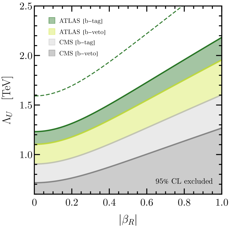
Figure 2: High-$p_{T}$ constraints on the $U_{1}$ model parameters $\beta_{R}$ and $\Lambda_{U}$ derived from the $pp\to\tau\bar{\tau}$ searches by CMS The CMS Collaboration (2022a) (gray) and ATLAS Aad et al. (2020) (green) in the $b$-tag and $b$-veto channels. The functional dependence is extracted using the HighPT package Allwicher et al. (2022b, a) and rescaled to the results presented in Ref. Haisch et al. (2022). The shaded regions correspond to the excluded parameter space at $95\,\%$ CL. The solid lines correspond to the constraints obtained using LHC run-II $(\sim 140\,\text{fb}^{-1})$ data, whereas the dashed line displays the projections for LHC’s high luminosity phase $(\sim 3\,\text{ab}^{-1})$ for the ATLAS $b$-tag search.

For our present study we use the HighPT package Allwicher et al. (2022b, a) to compute the $\chi^{2}$ likelihood of the EFT Lagrangian in Eq. (3) for the $b$-veto channel of the ATLAS di-tau search Aad et al. (2020). We then rescale this result to match the NLO predictions derived in Ref. Haisch et al. (2022) for the $U_{1}$ leptoquark for the ATLAS Aad et al. (2020) and CMS The CMS Collaboration (2022a) searches in both $b$-tag and $b$-veto channels.

Minimizing the rescaled $\chi^{2}$ likelihoods with respect to the right-handed coupling $\beta_{R}$ and the effective scale $\Lambda_{U}$, we find the $95\,\%$ CL exclusion regions shown in Fig. 2. The ATLAS di-tau search Aad et al. (2020), shown in green, provides stronger exclusion limits than the corresponding CMS search The CMS Collaboration (2022a), displayed in gray. This can be understood by noticing that a slight excess of events is observed in the high-$p_{T}$ tail in the latter search, weakening the constraints derived from it. For both collaborations, the $b$-tag channels (dark green/light gray) yield more stringent constraints than the corresponding $b$-veto channels (light green/dark gray), as anticipated. As previously mentioned, this is because the signal comes dominantly from the process $b\bar{b}\to\tau\bar{\tau}$, where at least one bottom quark is likely to come from gluon splitting $(g\to b\bar{b})$ allowing to require an associated $b$-jet, which significantly reduces the background and thus yields stronger constraints. Furthermore, it is evident that the scenarios with large right-handed currents $\beta_{R}$ are tightly constrained by high-$p_{T}$ data.

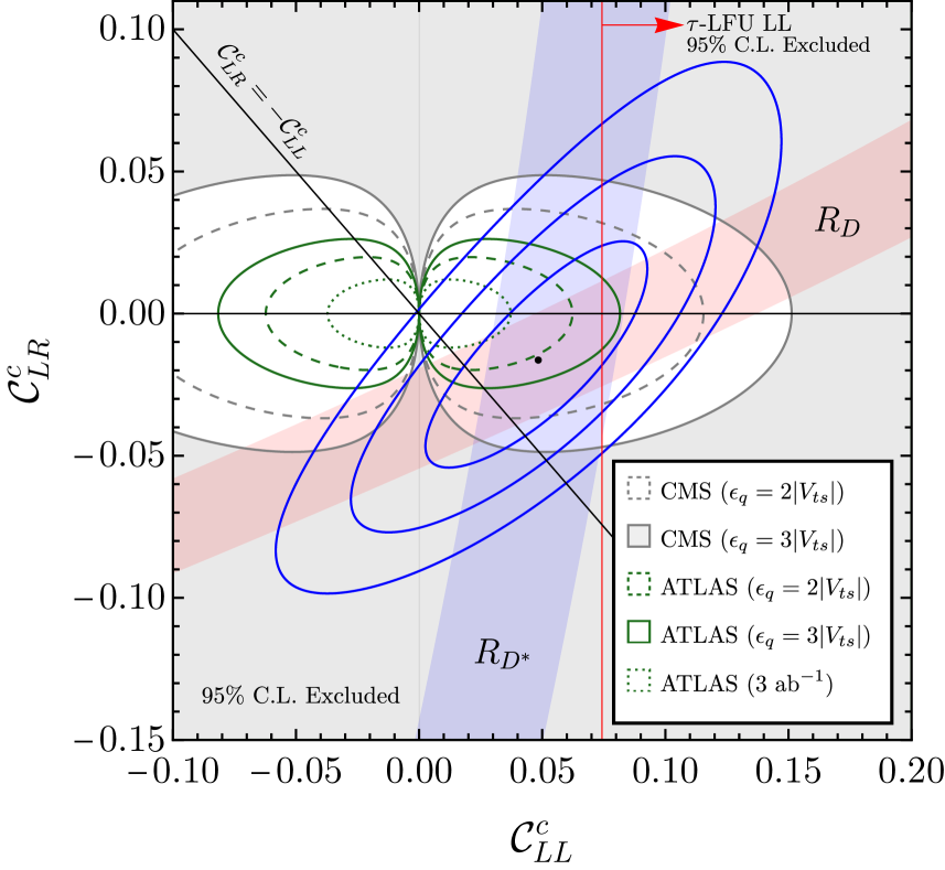
Figure 3: High-$p_{T}$ constraints superimposed on the low-energy fit. The red and blue bands represent the $\Delta\chi^{2}=1$ regions preferred by $R_{D}$ and $R_{D^{\ast}}$. The blue lines correspond to the $1\sigma$, $2\sigma$, and $3\sigma$ contours of the combined low-energy fit including all $b\rightarrow c$ observables (dot = best fit point). The high-$p_{T}$ exclusion limits derived from the $b$-tag channel of the CMS The CMS Collaboration (2022a) (ATLAS Aad et al. (2020)) search are given by regions outside of the gray (green) lines. On the other hand, the region inside the innermost dotted curve is our projection for the allowed parameter space from high-$p_{T}$ searches (in absence of a signal) with a luminosity of $3\,\text{ab}^{-1}$. Finally, the region to the right of the red line is excluded by $\tau$-LFU tests assuming leading log running of $C^{33\tau\tau}_{LL}$. See text for more details.

Next, we compare these high-$p_{T}$ results to the low-energy constraints derived in the previous section, by minimizing both likelihoods with respect to the Wilson coefficients $\mathcal{C}_{LL}^{c}$ and $\mathcal{C}_{LR}^{c}$, again evaluated at the reference high-scale $\Lambda_{\rm UV}=1$ TeV. The resulting fit is shown in Fig. 3, where the red and blue bands represent the preferred $\Delta\chi^{2}=1$ regions for the measurements of $R_{D}$ and $R_{D^{\ast}}$. The blue lines correspond to the $1\sigma$, $2\sigma$, and $3\sigma$ contours of the combined low-energy fit including all $b\rightarrow c$ observables, whereas the gray (green) lines indicate the $95\,\%$ CL exclusion contours for the CMS (ATLAS) di-tau search using the $b$-tag channel. The solid and dashed lines correspond to the constraints obtained assuming $\epsilon_{q}=3|V_{ts}|$ and $\epsilon_{q}=2|V_{ts}|$, respectively.

As can be seen, the high-energy constraints are already very close to the parameter region favored by low-energy data. To this purpose, it should be noted that scenarios with smaller $\epsilon_{q}$ are more constrained by high-$p_{T}$ as they require a lower scale $\Lambda_{U}$ to explain the charged-current anomalies (see Eq. (25)). On the other hand, values of $\epsilon_{q}$ larger than $3|V_{ts}|$ are both unnatural and highly disfavoured by $\Delta F=2$ constraints in UV complete models in the absence of fine-tuning.

Due to the excess of events currently observed by CMS, the corresponding limits are significantly weaker than those of ATLAS. If interpreted as a signal, the CMS excess (which is further supported by a dedicated $t$-channel analysis The CMS Collaboration (2022b)) would favour the parameter region close to the CMS exclusion bounds in Fig. 3. Given the low-energy constraints, this would in turn prefer a scenario with sizable right-handed couplings. On the other hand, ATLAS data are more compatible with low-energy data in the region of a pure left-handed coupling (though right-handed couplings remain viable).

Overall, the plot in Fig. 3 shows that low- and high-energy data yield complementary constraints, and that a $U_{1}$ explanation of $R_{D^{(*)}}$ is compatible with present $pp\to\tau\bar{\tau}$ data. This plot also shows that future high-energy data will play an essential role in testing the $U_{1}$ explanation of charged-current $B$ anomalies. To illustrate this point, we indicate the projection for an integrated luminosity of $3\,\text{ab}^{-1}$ by the shaded green central region in Fig. 3, which shows the potential of the high-luminosity phase of LHC assuming $\epsilon_{q}=2|V_{ts}|$. The projection was derived using the ATLAS $b$-tag search assuming that background uncertainties scale as the square-root of the luminosity. This projection shows that a large part of the relevant parameter space will be probed with the data sets expected from Run-III and the LHC high-luminosity phase.

For completeness, in Fig. 3 we also indicate the region disfavoured by LFU tests in $\tau$ decays Feruglio et al. (2017): the region to the right of the red line is excluded by the experimental determination of $(g_{\tau}^{W}/g^{W}_{\mu,e})_{\ell,\pi,K}$  Amhis et al. (2021), using the leading-log (LL) running of $C^{33\tau\tau}_{LL}(1~{}{\rm TeV})$ Feruglio et al. (2017), and setting $\epsilon_{q}=3|V_{ts}|$ (most conservative choice). Due to their purely left-handed nature, $\tau$-LFU tests provide a strong constraint on the left-handed only hypothesis, potentially favouring scenarios with right-handed currents. However, this point comes with the caveat that additional contributions from new states in UV complete models can soften these bounds Allwicher et al. (2022c).

IV Conclusions

In this paper we have analyzed the compatibility of the $U_{1}$ LQ explanation of the charged-current $B$-meson anomalies in light of new low- and high-energy data. To this purpose, we have first re-analysed in a bottom-up and, to large extent, model-independent approach the assumptions necessary to relate the $U_{1}$ couplings appearing in $b\to c\tau\bar{\nu}$, $b\to u\tau\bar{\nu}$, and $b\bar{b}\to\tau\bar{\tau}$ transitions.

Updating the fit to the low-energy data, we find that the region preferred by $b\rightarrow c$ observables is equally compatible with a purely left-handed interaction, as well as with a scenario with right-handed currents of equal magnitude. The latter option is quite interesting, given sizable right-handed currents are a distinctive signature of models where the $U_{1}$ is embedded in a flavor non-universal gauge group Bordone et al. (2018). In both cases, the pull of the $U_{1}$ hypothesis is at the $3\sigma$ level. The present low-energy fit already highlights the role of $B_{u}\rightarrow\tau\bar{\nu}$ in pinning down the residual uncertainty on the flavor structure of the $U_{1}$ couplings. Indeed, this observable is expected to play an even more important role in the near future with the help of new data coming from Belle-II Altmannshofer et al. (2019).

Next, we examined collider constraints on the model, focusing on the $pp\to\tau\bar{\tau}$ Drell-Yan production channel mediated by $t$-channel $U_{1}$ exchange that provides the most stringent bounds. By superimposing these limits on the parameter space preferred by the low-energy fit, we conclude that constraints coming from the high-energy $pp\to\tau\bar{\tau}$ process are already closing in on the low-energy parameter space preferred by the charged-current $B$-meson anomalies.

While low- and high-energy data are currently well compatible, a large fraction of the viable parameter space will be probed by the high-luminosity phase of the LHC. This is especially true in the case of equal magnitude left- and right-handed currents (${\mathcal{C}}^{c}_{LL}=-{\mathcal{C}}^{c}_{LR}$), which has become more viable with the updated low-energy data and will be probed at the 95% confidence level by the LHC. This will provide an exciting test of the well-motivated class of UV completions for the $U_{1}$ based on non-universal gauge groups, featuring quark-lepton unification for the third family at the TeV scale Bordone et al. (2018); Greljo and Stefanek (2018); Fuentes-Martín and Stangl (2020); Fuentes-Martin et al. (2022).

Note Added

While this project was under completion, an independent phenomenological analysis of charged-current $B$-meson anomalies, including different leptoquark interpretations, has appeared Iguro et al. (2022). Our results in Sect. III (low-energy fit) are compatible with those presented in Iguro et al. (2022).

Appendix A Preferred regions for $U_{1}$ couplings

In view of future searches of $U_{1}$ signals in channels involving $\tau$ leptons, both at high and at low energies, we provide here a summary of the preferred parameter-space region resulting from the low-energy fit performed in this paper. We also report predictions for ${\mathcal{B}}(B_{s}\to\tau^{+}\tau^{-})$ and ${\mathcal{B}}(B^{+}\to K^{+}\tau^{+}\tau^{-})$, which can be considered the low-energy counterparts of $pp\to\tau\bar{\tau}$.

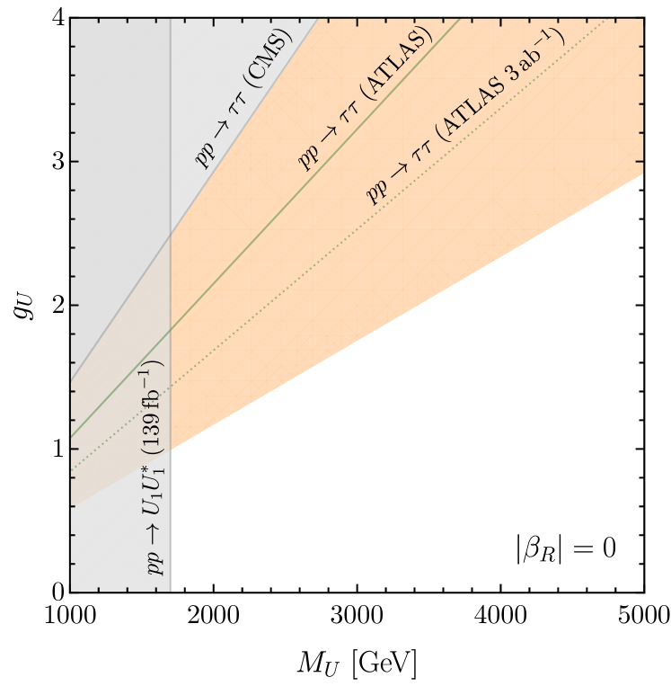
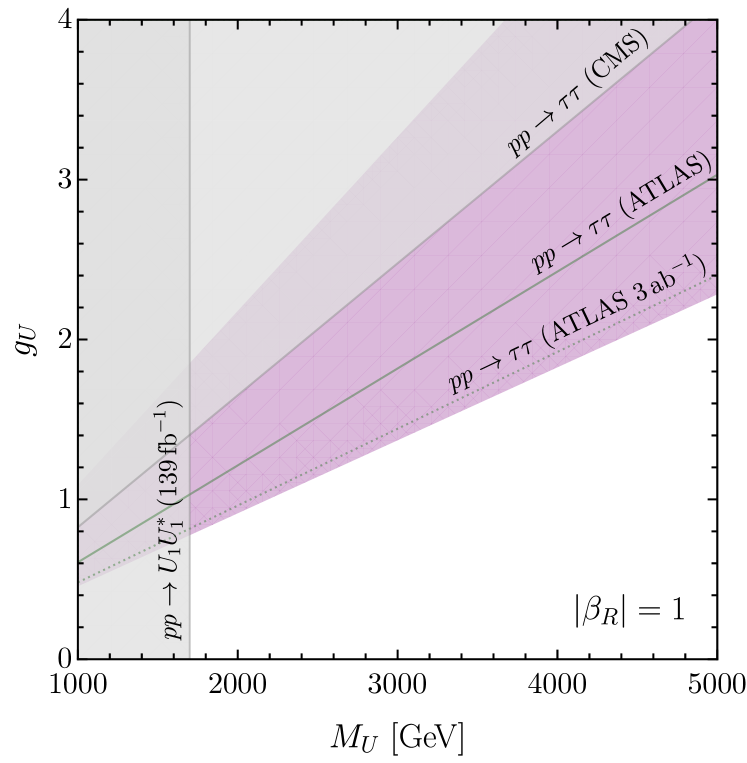
Figure 4: Preferred region at 90% CL from low-energy charged-current data for mass ($M_{U}$) and leading fermion coupling ($g_{U}$) of the $U_{1}$ LQ. Top: Purely left-handed case ($\beta_{R}=0$). Bottom: Pati-Salam-like case ($|\beta_{R}|=1$). The gray region and solid lines indicate constraints of present high-energy searches at 95% CL, while the dotted line gives the projected sensitivity at the HL-LHC with a luminosity of $3\,{\rm ab}^{-1}$.

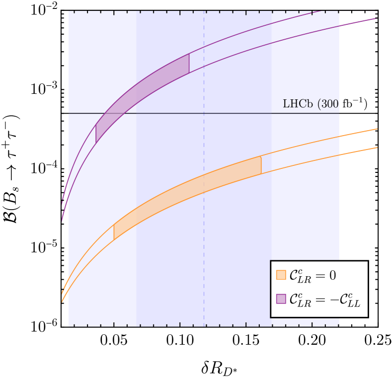
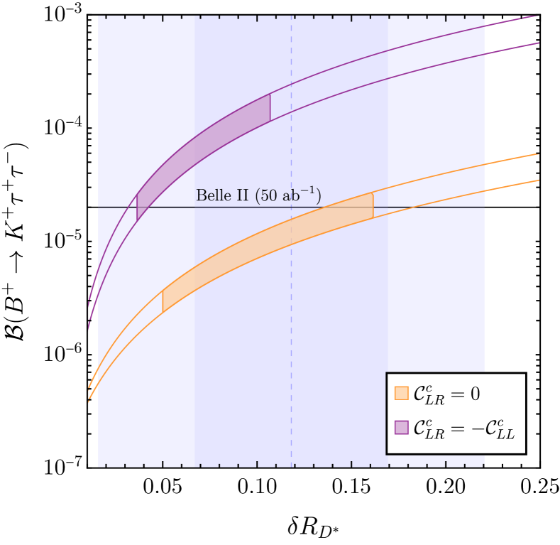
Figure 5: Predicted ranges for ${\mathcal{B}}(B_{s}\rightarrow\tau^{+}\tau^{-})$ and ${\mathcal{B}}(B^{+}\to K^{+}\tau^{+}\tau^{-})$ as a function of $\delta R_{D^{*}}=R_{D^{*}}/R_{D^{*}}^{\text{SM}}-1$. The filled orange and purple colored regions correspond to the 90% CL preferred regions from the low-energy charged-current fit. The blue vertical bands denote the present $1\sigma$ and $2\sigma$ experimental ranges for $\delta R_{D^{*}}$.

The effective interaction between the $U_{1}$ field and fermion currents involving the $\tau$ lepton is $\mathcal{L}_{\rm int}=U_{\mu}J^{\mu}_{U}$, with $J^{\mu}_{U}$ defined as in (17). By convention, we set $\beta_{L}^{b\tau}=1$. The parameter $\beta_{R}$, which characterises different UV completions of the effective interaction with right-handed fermions, should be treated as a free parameter. In order to define precise benchmarks, we consider two reference cases for $\beta_{R}$:

1. $|\beta_{R}|=0$ (Purely left-handed case)
   Values preferred by low-energy data at 90% CL:

   $$M_{U}/g_{U} \in[0.69~{}{\rm TeV},\,1.71~{}{\rm TeV}]\,,$$ (37)

2. $|\beta_{R}|=1$ (Pati-Salam-like LQ)
   Values preferred by low-energy data at 90% CL:

   $$M_{U}/g_{U} \in[0.92~{}{\rm TeV},\,2.19~{}{\rm TeV}]\,.$$ (38)

In Fig. 4 we show the present and future exclusion bounds in the $g_{U}$ vs. $M_{U}$ plane from high-energy searches, as well as the region preferred by the low-energy fit corresponding to (37) and (38).

As discussed in the main text, low-energy data on charged currents alone are not able to provide a stringent constraint on $\beta_{s\tau}$. However, the latter is constrained by $\Delta M_{B_{s}}$ under general assumptions about the UV completion. The range we consider motivated in view of future experimental searches is

$$\beta_{s\tau}\in[0.06,\,0.16]\,,$$ (39)

The $g_{U}/M_{U}$ ranges reported in (37) and (38) are obtained under this assumption, and setting $\beta_{d\tau}=0$.

The theoretical expression for $B^{+}\to K^{+}\tau^{+}\tau^{-}$ reads Cornella et al. (2021)

$$10^{9}{\mathcal{B}}(B^{+}\to K^{+}\tau^{+}\tau^{-})=2.2|{\mathcal{C}}_{9}^{s\tau}|^{2}+6.0|{\mathcal{C}}_{10}^{s\tau}|^{2}+8.3|{\mathcal{C}}_{S}^{s\tau}|^{2}$$

$$+8.9|{\mathcal{C}}_{P}^{s\tau}|^{2}+4.8{\rm Re}\left({\mathcal{C}}_{S}^{s\tau}{\mathcal{C}}_{9}^{s\tau*}\right)+5.9{\rm Re}\left({\mathcal{C}}_{P}^{s\tau}{\mathcal{C}}_{10}^{s\tau*}\right)\,,$$ (40)

where ${\mathcal{C}}_{9}^{s\tau}={\mathcal{C}}_{\rm 9,SM}+{\mathcal{C}}_{\rm 9,NP}^{s\tau}$ and ${\mathcal{C}}_{10}^{s\tau}={\mathcal{C}}_{\rm 10,SM}+{\mathcal{C}}_{\rm 10,NP}^{s\tau}$, with ${\mathcal{C}}_{\rm 9,SM}=4.1$ and ${\mathcal{C}}_{\rm 10,SM}=-4.2$.

In terms of the Wilson coefficients of ${\mathcal{L}}^{\rm LQ}_{\rm EFT}$, the coefficients appearing in (40) read

$${\mathcal{C}}_{\rm 9,NP}^{s\tau}=-{\mathcal{C}}_{\rm 10,NP}^{s\tau} =-\frac{2\pi}{\alpha V_{ts}^{*}V_{tb}}{\mathcal{C}}_{LL}^{sb\tau\tau}\,,$$ (41)

$${\mathcal{C}}_{S}^{s\tau}=-{\mathcal{C}}_{P}^{s\tau} =\frac{4\pi}{\alpha V_{ts}^{*}V_{tb}}{\mathcal{C}}_{LR}^{sb\tau\tau}\,.$$ (42)

As far as $B_{s}\rightarrow\tau^{+}\tau^{-}$ is concerned, the branching fraction can be decomposed as

$$\frac{\mathcal{B}(B_{s}\rightarrow\tau^{+}\tau^{-})}{\mathcal{B}(B_{s}\rightarrow\tau^{+}\tau^{-})_{\rm SM}}=\bigg{|}1+\frac{{\mathcal{C}}_{\rm 10,NP}^{s\tau}}{{\mathcal{C}}_{\rm 10,SM}}+\frac{\chi_{s\tau}{\mathcal{C}}_{P}^{s\tau}}{{\mathcal{C}}_{\rm 10,SM}}\bigg{|}^{2}$$

$$+\left(1-\frac{4m_{\tau}^{2}}{m_{B_{s}}^{2}}\right)\bigg{|}\frac{\chi_{s\tau}{\mathcal{C}}_{S}^{s\tau}}{{\mathcal{C}}_{\rm 10,SM}}\bigg{|}^{2} \,,$$ (43)

where we have defined the chiral enhancement factor

$$\chi_{s\tau}=\frac{m_{B_{s}}^{2}}{2m_{\tau}(m_{b}+m_{s})}\,.$$ (44)

The model predictions for ${\mathcal{B}}(B_{s}\rightarrow\tau^{+}\tau^{-})$ and ${\mathcal{B}}(B^{+}\to K^{+}\tau^{+}\tau^{-})$ corresponding to the two ranges in (37) and (38), as well as the flat range on $\beta_{s\tau}$ in (39), are shown in Fig. 5.

References

- Alonso et al. (2015) R. Alonso, B. Grinstein, and J. Martin Camalich, JHEP 10, 184 (2015), arXiv:1505.05164 [hep-ph] .
- Calibbi et al. (2015) L. Calibbi, A. Crivellin, and T. Ota, Phys. Rev. Lett. 115, 181801 (2015), arXiv:1506.02661 [hep-ph] .
- Barbieri et al. (2016) R. Barbieri, G. Isidori, A. Pattori, and F. Senia, Eur. Phys. J. C 76, 67 (2016), arXiv:1512.01560 [hep-ph] .
- Bhattacharya et al. (2017) B. Bhattacharya, A. Datta, J.-P. Guévin, D. London, and R. Watanabe, JHEP 01, 015 (2017), arXiv:1609.09078 [hep-ph] .
- Buttazzo et al. (2017) D. Buttazzo, A. Greljo, G. Isidori, and D. Marzocca, JHEP 11, 044 (2017), arXiv:1706.07808 [hep-ph] .
- Kumar et al. (2019) J. Kumar, D. London, and R. Watanabe, Phys. Rev. D 99, 015007 (2019), arXiv:1806.07403 [hep-ph] .
- Angelescu et al. (2018) A. Angelescu, D. Bečirević, D. A. Faroughy, and O. Sumensari, JHEP 10, 183 (2018), arXiv:1808.08179 [hep-ph] .
- Pati and Salam (1974) J. C. Pati and A. Salam, Phys. Rev. D 10, 275 (1974), [Erratum: Phys.Rev.D 11, 703–703 (1975)].
- Di Luzio et al. (2017) L. Di Luzio, A. Greljo, and M. Nardecchia, Phys. Rev. D 96, 115011 (2017), arXiv:1708.08450 [hep-ph] .
- Bordone et al. (2018) M. Bordone, C. Cornella, J. Fuentes-Martin, and G. Isidori, Phys. Lett. B 779, 317 (2018), arXiv:1712.01368 [hep-ph] .
- Greljo and Stefanek (2018) A. Greljo and B. A. Stefanek, Phys. Lett. B 782, 131 (2018), arXiv:1802.04274 [hep-ph] .
- Di Luzio et al. (2018) L. Di Luzio, J. Fuentes-Martin, A. Greljo, M. Nardecchia, and S. Renner, JHEP 11, 081 (2018), arXiv:1808.00942 [hep-ph] .
- Fuentes-Martín et al. (2020a) J. Fuentes-Martín, G. Isidori, M. König, and N. Selimović, Phys. Rev. D 101, 035024 (2020a), arXiv:1910.13474 [hep-ph] .
- Fuentes-Martín et al. (2020b) J. Fuentes-Martín, G. Isidori, M. König, and N. Selimović, Phys. Rev. D 102, 115015 (2020b), arXiv:2009.11296 [hep-ph] .
- Cornella et al. (2019) C. Cornella, J. Fuentes-Martin, and G. Isidori, JHEP 07, 168 (2019), arXiv:1903.11517 [hep-ph] .
- Cornella et al. (2021) C. Cornella, D. A. Faroughy, J. Fuentes-Martin, G. Isidori, and M. Neubert, JHEP 08, 050 (2021), arXiv:2103.16558 [hep-ph] .
- Panico and Pomarol (2016) G. Panico and A. Pomarol, JHEP 07, 097 (2016), arXiv:1603.06609 [hep-ph] .
- Allwicher et al. (2021) L. Allwicher, G. Isidori, and A. E. Thomsen, JHEP 01, 191 (2021), arXiv:2011.01946 [hep-ph] .
- Barbieri (2021) R. Barbieri, Acta Phys. Polon. B 52, 789 (2021), arXiv:2103.15635 [hep-ph] .
- Fuentes-Martín and Stangl (2020) J. Fuentes-Martín and P. Stangl, Phys. Lett. B 811, 135953 (2020), arXiv:2004.11376 [hep-ph] .
- Fuentes-Martin et al. (2021) J. Fuentes-Martin, G. Isidori, J. Pagès, and B. A. Stefanek, Phys. Lett. B 820, 136484 (2021), arXiv:2012.10492 [hep-ph] .
- Fuentes-Martin et al. (2022) J. Fuentes-Martin, G. Isidori, J. M. Lizana, N. Selimovic, and B. A. Stefanek, Phys. Lett. B 834, 137382 (2022), arXiv:2203.01952 [hep-ph] .
- Assad et al. (2018) N. Assad, B. Fornal, and B. Grinstein, Phys. Lett. B 777, 324 (2018), arXiv:1708.06350 [hep-ph] .
- Calibbi et al. (2018) L. Calibbi, A. Crivellin, and T. Li, Phys. Rev. D 98, 115002 (2018), arXiv:1709.00692 [hep-ph] .
- Barbieri and Tesi (2018) R. Barbieri and A. Tesi, Eur. Phys. J. C 78, 193 (2018), arXiv:1712.06844 [hep-ph] .
- Blanke and Crivellin (2018) M. Blanke and A. Crivellin, Phys. Rev. Lett. 121, 011801 (2018), arXiv:1801.07256 [hep-ph] .
- Balaji et al. (2019) S. Balaji, R. Foot, and M. A. Schmidt, Phys. Rev. D 99, 015029 (2019), arXiv:1809.07562 [hep-ph] .
- Dolan et al. (2021) M. J. Dolan, T. P. Dutka, and R. R. Volkas, JHEP 05, 199 (2021), arXiv:2012.05976 [hep-ph] .
- King (2021) S. F. King, JHEP 11, 161 (2021), arXiv:2106.03876 [hep-ph] .
- Fernández Navarro and King (2022) M. Fernández Navarro and S. F. King, (2022), arXiv:2209.00276 [hep-ph] .
- Angelescu et al. (2021) A. Angelescu, D. Bečirević, D. A. Faroughy, F. Jaffredo, and O. Sumensari, Phys. Rev. D 104, 055017 (2021), arXiv:2103.12504 [hep-ph] .
- Bhaskar et al. (2021) A. Bhaskar, D. Das, T. Mandal, S. Mitra, and C. Neeraj, Phys. Rev. D 104, 035016 (2021), arXiv:2101.12069 [hep-ph] .
- Barbieri et al. (2022) R. Barbieri, C. Cornella, and G. Isidori, (2022), arXiv:2207.14248 [hep-ph] .
- Haisch et al. (2022) U. Haisch, L. Schnell, and S. Schulte, (2022), arXiv:2209.12780 [hep-ph] .
- (35) G. M. Ciezarek (LHCb), CERN Seminar, https://indico.cern.ch/event/1187939/ .
- The CMS Collaboration (2022a) The CMS Collaboration (CMS), (2022a), arXiv:2208.02717 [hep-ex] .
- The CMS Collaboration (2022b) The CMS Collaboration (CMS), CMS-PAS-EXO-19-016 (2022b).
- Faroughy et al. (2017) D. A. Faroughy, A. Greljo, and J. F. Kamenik, Phys. Lett. B 764, 126 (2017), arXiv:1609.07138 [hep-ph] .
- Aad et al. (2020) G. Aad et al. (ATLAS), Phys. Rev. Lett. 125, 051801 (2020), arXiv:2002.12223 [hep-ex] .
- Fuentes-Martín et al. (2020c) J. Fuentes-Martín, G. Isidori, J. Pagès, and K. Yamamoto, Phys. Lett. B 800, 135080 (2020c), arXiv:1909.02519 [hep-ph] .
- Barbieri et al. (2011) R. Barbieri, G. Isidori, J. Jones-Perez, P. Lodone, and D. M. Straub, Eur. Phys. J. C 71, 1725 (2011), arXiv:1105.2296 [hep-ph] .
- Barbieri et al. (2012) R. Barbieri, D. Buttazzo, F. Sala, and D. M. Straub, JHEP 07, 181 (2012), arXiv:1203.4218 [hep-ph] .
- Crosas et al. (2022) O. L. Crosas, G. Isidori, J. M. Lizana, N. Selimovic, and B. A. Stefanek, (2022), arXiv:2207.00018 [hep-ph] .
- Baker et al. (2019) M. J. Baker, J. Fuentes-Martín, G. Isidori, and M. König, Eur. Phys. J. C 79, 334 (2019), arXiv:1901.10480 [hep-ph] .
- Alonso et al. (2017) R. Alonso, B. Grinstein, and J. Martin Camalich, Phys. Rev. Lett. 118, 081802 (2017), arXiv:1611.06676 [hep-ph] .
- Aaij et al. (2023a) R. Aaij et al. (LHCb), (2023a), arXiv:2302.02886 [hep-ex] .
- Aaij et al. (2023b) R. Aaij et al. (LHCb), https://indico.cern.ch/event/1231797 (2023b).
- Amhis et al. (2021) Y. S. Amhis et al. (HFLAV [https://hflav.web.cern.ch]), Eur. Phys. J. C 81, 226 (2021), arXiv:1909.12524 [hep-ex] .
- Bailey et al. (2015) J. A. Bailey et al. (MILC), Phys. Rev. D 92, 034506 (2015), arXiv:1503.07237 [hep-lat] .
- Na et al. (2015) H. Na, C. M. Bouchard, G. P. Lepage, C. Monahan, and J. Shigemitsu (HPQCD), Phys. Rev. D 92, 054510 (2015), [Erratum: Phys.Rev.D 93, 119906 (2016)], arXiv:1505.03925 [hep-lat] .
- Bernlochner et al. (2017) F. U. Bernlochner, Z. Ligeti, M. Papucci, and D. J. Robinson, Phys. Rev. D 95, 115008 (2017), [Erratum: Phys.Rev.D 97, 059902 (2018)], arXiv:1703.05330 [hep-ph] .
- Gambino et al. (2019) P. Gambino, M. Jung, and S. Schacht, Phys. Lett. B 795, 386 (2019), arXiv:1905.08209 [hep-ph] .
- Bordone et al. (2020) M. Bordone, M. Jung, and D. van Dyk, Eur. Phys. J. C 80, 74 (2020), arXiv:1908.09398 [hep-ph] .
- Martinelli et al. (2022) G. Martinelli, S. Simula, and L. Vittorio, Phys. Rev. D 105, 034503 (2022), arXiv:2105.08674 [hep-ph] .
- Bečirević and Jaffredo (2022) D. Bečirević and F. Jaffredo, (2022), arXiv:2209.13409 [hep-ph] .
- Aaij et al. (2022) R. Aaij et al. (LHCb), Phys. Rev. Lett. 128, 191803 (2022), arXiv:2201.03497 [hep-ex] .
- Workman et al. (2022) R. L. Workman et al. (Particle Data Group), PTEP 2022, 083C01 (2022).
- Bona et al. (2022) M. Bona et al. (UTfit [http://www.utfit.org/UTfit/]), PoS EPS-HEP2021, 500 (2022).
- Aebischer et al. (2017) J. Aebischer, M. Fael, C. Greub, and J. Virto, JHEP 09, 158 (2017), arXiv:1704.06639 [hep-ph] .
- Crivellin et al. (2019) A. Crivellin, C. Greub, D. Müller, and F. Saturnino, Phys. Rev. Lett. 122, 011805 (2019), arXiv:1807.02068 [hep-ph] .
- London and Matias (2022) D. London and J. Matias, Ann. Rev. Nucl. Part. Sci. 72, 37 (2022), arXiv:2110.13270 [hep-ph] .
- Altmannshofer and Stangl (2021) W. Altmannshofer and P. Stangl, Eur. Phys. J. C 81, 952 (2021), arXiv:2103.13370 [hep-ph] .
- Cornella et al. (2020) C. Cornella, G. Isidori, M. König, S. Liechti, P. Owen, and N. Serra, Eur. Phys. J. C 80, 1095 (2020), arXiv:2001.04470 [hep-ph] .
- Khodjamirian et al. (2013) A. Khodjamirian, T. Mannel, and Y. M. Wang, JHEP 02, 010 (2013), arXiv:1211.0234 [hep-ph] .
- Allwicher et al. (2022a) L. Allwicher, D. A. Faroughy, F. Jaffredo, O. Sumensari, and F. Wilsch, (2022a), arXiv:2207.10714 [hep-ph] .
- Diaz et al. (2017) B. Diaz, M. Schmaltz, and Y.-M. Zhong, JHEP 10, 097 (2017), arXiv:1706.05033 [hep-ph] .
- Blumlein et al. (1997) J. Blumlein, E. Boos, and A. Kryukov, Z. Phys. C 76, 137 (1997), arXiv:hep-ph/9610408 .
- Doršner and Greljo (2018) I. Doršner and A. Greljo, JHEP 05, 126 (2018), arXiv:1801.07641 [hep-ph] .
- Aad et al. (2021) G. Aad et al. (ATLAS), Phys. Rev. D 104, 112005 (2021), arXiv:2108.07665 [hep-ex] .
- Sirunyan et al. (2021) A. M. Sirunyan et al. (CMS), Phys. Lett. B 819, 136446 (2021), arXiv:2012.04178 [hep-ex] .
- Hammett and Ross (2015) J. B. Hammett and D. A. Ross, JHEP 07, 148 (2015), arXiv:1501.06719 [hep-ph] .
- Mandal et al. (2015) T. Mandal, S. Mitra, and S. Seth, JHEP 07, 028 (2015), arXiv:1503.04689 [hep-ph] .
- Alves et al. (2003) A. Alves, O. Eboli, and T. Plehn, Phys. Lett. B 558, 165 (2003), arXiv:hep-ph/0211441 .
- Haisch and Polesello (2021) U. Haisch and G. Polesello, JHEP 05, 057 (2021), arXiv:2012.11474 [hep-ph] .
- Buonocore et al. (2020a) L. Buonocore, U. Haisch, P. Nason, F. Tramontano, and G. Zanderighi, Phys. Rev. Lett. 125, 231804 (2020a), arXiv:2005.06475 [hep-ph] .
- Greljo and Selimovic (2021) A. Greljo and N. Selimovic, JHEP 03, 279 (2021), arXiv:2012.02092 [hep-ph] .
- Buonocore et al. (2020b) L. Buonocore, P. Nason, F. Tramontano, and G. Zanderighi, JHEP 08, 019 (2020b), arXiv:2005.06477 [hep-ph] .
- Buonocore et al. (2022) L. Buonocore, A. Greljo, P. Krack, P. Nason, N. Selimovic, F. Tramontano, and G. Zanderighi, (2022), arXiv:2209.02599 [hep-ph] .
- Allwicher et al. (2022b) L. Allwicher, D. A. Faroughy, F. Jaffredo, O. Sumensari, and F. Wilsch, (2022b), arXiv:2207.10756 [hep-ph] .
- Feruglio et al. (2017) F. Feruglio, P. Paradisi, and A. Pattori, JHEP 09, 061 (2017), arXiv:1705.00929 [hep-ph] .
- Allwicher et al. (2022c) L. Allwicher, G. Isidori, and N. Selimovic, Phys. Lett. B 826, 136903 (2022c), arXiv:2109.03833 [hep-ph] .
- Altmannshofer et al. (2019) W. Altmannshofer et al. (Belle-II), PTEP 2019, 123C01 (2019), [Erratum: PTEP 2020, 029201 (2020)], arXiv:1808.10567 [hep-ex] .
- Iguro et al. (2022) S. Iguro, T. Kitahara, and R. Watanabe, (2022), arXiv:2210.10751 [hep-ph] .