Razor-thin dust layers in protoplanetary disks:
Limits on the vertical shear instability

Context: Recent observations with the Atacama Large Millimeter Array (ALMA) have shown that the large dust aggregates observed at millimeter wavelengths settle to the midplane into a remarkably thin layer. This sets strong limits on the strength of the turbulence and other gas motions in these disks.
Aims: We intend to find out if the geometric thinness of these layers is evidence against the vertical shear instability (VSI) operating in these disks. We aim to verify if a dust layer consisting of large enough dust aggregates could remain geometrically thin enough to be consistent with the latest observations of these dust layers, even if the disk is unstable to the VSI. If this is falsified, then the observed flatness of these dust layers proves that these disks are stable against the VSI, even out to the large radii at which these dust layers are observed.
Methods: We performed hydrodynamic simulations of a protoplanetary disk with a locally isothermal equation of state, and let the VSI fully develop. We sprinkled dust particles with a given grain size at random positions near the midplane and followed their motion as they got stirred up by the VSI, assuming no feedback onto the gas. We repeated the experiment for different grain sizes and determined for which grain size the layer becomes thin enough to be consistent with ALMA observations. We then verified if, with these grain sizes, it is still possible (given the constraints of dust opacity and gravitational stability) to generate a moderately optically thick layer at millimeter wavelengths, as observations appear to indicate.
Results: We found that even very large dust aggregates with Stokes numbers close to unity get stirred up to relatively large heights above the midplane by the VSI, which is in conflict with the observed geometric thinness. For grains so large that the Stokes number exceeds unity, the layer can be made to remain thin, but we show that it is hard to make dust layers optically thick at ALMA wavelengths (e.g., $\tau_{\mathrm{1.3mm}}\gtrsim 1$) with such large dust aggregates.
Conclusions: We conclude that protoplanetary disks with geometrically thin midplane dust layers cannot be VSI unstable, at least not down to the disk midplane. Explanations for the inhibition of the VSI out to several hundreds of au include a high dust-to-gas ratio of the midplane layer, a modest background turbulence, and/or a reduced dust-to-gas ratio of the small dust grains that are responsible for the radiative cooling of the disk. A reduction of small grains by a factor of between 10 and 100 is sufficient to quench the VSI. Such a reduction is plausible in dust growth models, and still consistent with observations at optical and infrared wavelengths.

ccretion, accretion disks – protoplanetary disks

1 Introduction

According to canonical theory, the evolution of protoplanetary disks is thought to be driven by a combination of viscous evolution and photoevaporation (e.g., Clarke et al., 2001). The viscosity in such disks is thought to be caused by turbulence produced by the magnetorotational instability (MRI). While the MRI is inhibited in very dense regions of the disk (the so-called dead zones), it may still be operational in the hot inner regions ($r\ll 1\,\mathrm{au}$), in the irradiated surface layers, and in the weakly ionized outer regions ($r\gg 1\,\mathrm{au}$) of the disk (e.g., Dzyurkevich et al., 2013).

However, in recent years the turbulent viscous disk theory for the outer regions of protoplanetary disks has been called into question. Using radiative transfer modeling of the Atacama Large Millimeter Array (ALMA) image of HL Tau, Pinte et al. (2016) infer that the turbulence in that disk must be weak ($\alpha\lesssim 10^{-3}$). Direct measurements of the turbulent line width in CO 2-1 with ALMA show mostly upper limits to the turbulent velocities of $\lesssim 10\%$ of the local sound speed (e.g., Flaherty et al., 2020). While these velocity upper limits are still consistent with turbulent $\alpha$ values of up to $10^{-2}$, and marginally consistent with MRI-turbulent disks (Flock et al., 2017), these and other measurements have stimulated the exploration of the possible consequences of the absence of MRI turbulence in protoplanetary disks and, consequently, the possibility that these disks may be much less turbulent than previously thought.

The implications of very low turbulent $\alpha$ values for protoplanetary disks are numerous. For instance, Bae et al. (2017) show that in low-$\alpha$ disks a single planet can produce multiple rings. Indeed, Zhang et al. (2018) demonstrate that a protoplanetary disk model with very low $\alpha$ and a single embedded planet can reproduce the observed many-ringed structure of the disk around AS 209 remarkably well (see, however Ziampras et al., 2020). Low turbulent velocities also have strong implications for dust growth, gap formation, planet migration, and many other things. The reason why, until not long ago, turbulent $\alpha$ values of $\lesssim 10^{-3}$ were not seriously considered by scientists in the field is that most stars with protoplanetary disks are observed to undergo substantial gas accretion. This requires $\alpha$ values in excess of about $10^{-3}$ (e.g. Hartmann et al., 1998). However, wind-driven accretion may provide a solution to this dilemma (e.g., Ferreira & Pelletier, 1995; Tabone et al., 2021; Martel & Lesur, 2022).

In the absense of the MRI, a protoplanetary disk can be prone to other, non-magnetohydrodynamic instabilities that cause turbulence or turbulence-like velocity fluctuations (e.g., Pfeil & Klahr, 2019). Of particular importance in the outer regions of the protoplanetary disk is the vertical shear instability (VSI, e.g. Nelson et al., 2013; Stoll & Kley, 2014, 2016; Flores-Rivera et al., 2020). This instability, when fully developed, produces upward and downward vertical streams of gas that slowly oscillate. These oscillations form a radially propagating wave (Svanberg et al., 2022). When viewed as a kind of turbulence, it is highly anisotropic, with turbulent “eddies” being radially narrow, but vertically extended sheets of gas moving either up or down. This “turbulence” is only weakly effective as a replacement of MRI turbulence for the radial transport of angular momentum, with values on the order of $\alpha_{\mathrm{VSI,radial}}\sim 10^{-4}$ (Stoll & Kley, 2014). However, due to the strong upward and downward motions of the gas, crossing the midplane, with velocities in the range of 5% to 20% of the isothermal sound speed, the effect of the VSI on the dust population of the disk is very pronounced (Stoll & Kley, 2016; Flock et al., 2017; Lin, 2019; Lehmann & Lin, 2022). Even large dust particles can be stirred up to high elevations above the midplane.

From the observational side, however, there is now increasing evidence that many, if not most, protoplanetary disks contain a layer of large dust aggregates at the midplane that contains a substantial amount of dust mass and is geometrically extremely flat, i.e., having a very small scale height. The first evidence came from the ALMA image of the disk around HL Tau, where radiative transfer modeling put an upper limit on the vertical scale height of the dust layer of 1 au at a radius of 100 au (Pinte et al., 2016). The high resolution ALMA images of the DSHARP campaign (Andrews et al., 2018) also suggest very flat geometries of the dust layers seen at $\lambda=1.3\,\mathrm{mm}$ wavelengths. Detailed radiative transfer analysis of the DSHARP observations of HD 163296 shows that the dust in the inner ring of that source (at $r\simeq 67\,\mathrm{au}$) appears to be vertically extended almost to the gas pressure scale height, but the outer ring (at $r\simeq 100\,\mathrm{au}$) appears to be less than 10% of the gas pressure scale height, i.e., highly settled (Doi & Kataoka, 2021).

To get better constraints on the vertical extent (geometric thickness) of the midplane dust layers of protoplanetary disks, dedicated observing campaigns with ALMA for nearly-edge-on disks are required. The first such campaign already yielded indications of strong settling of large grains (Villenave et al., 2020). But when the disk of Oph 163131 was reobserved with ALMA by Villenave et al. (2022), the vertical scale height of the dust layer could be constrained to be less than 0.5 au at a radius of 100 au, which is about 7% of the gas pressure scale height at that radius. From these observations, and under some assumptions of the grain size, these authors derive an upper limit of $\alpha\lesssim 10^{-5}$ on the turbulence.

However, if the VSI is operational in these outer disk regions, one might expect that the dust layer should be much more vertically extended, due to the high efficiency of the vertical dust stirring of the VSI. The purpose of this paper is to quantify this.

The grain sizes are not perfectly known, nor is the gas disk density. We address the question whether the grains could be so large that they remain in a thin layer in spite of the VSI. And if not, what could be the reason that the VSI is not operational in this disk.

The paper is structured as follows: We start with an analysis of the stirring-up of particles in Section 2. In Section 3 we explain why $\mathrm{St}\gg 1$ particles are not a probable explanation for the thin dust layers. We propose a natural explanation for the absense of VSI in protoplanetary disks in Section 4, and we finish with a discussion and conclusions.

2 Stirring up of large dust aggregates by the VSI

In this paper we wish to find out if the presence of the VSI in the outer regions of a protoplanetary disk, such as the one around Oph 163131, would inevitably lead to the big-grain dust layer observed with ALMA to be more geometrically extended than observed. This would then be clear evidence that the VSI does not operate in that disk.

The effect of the VSI on dust particles in the disk was studied by several papers (e.g., Lorén-Aguilar & Bate, 2015; Stoll & Kley, 2016; Flock et al., 2017; Lehmann & Lin, 2022). The models we present in this section are fundamentally different from those earlier papers. However, we explore the parameters and compare the results to the observational constraints.

2.1 Conveyor-belt estimate of vertical mixing efficiency of the VSI

A simple estimate of the height above the midplane that a dust aggregate can be lifted by the VSI would be the following. Assume that the VSI consists of long-lived vertical upward and downward moving slabs of gas, acting as vertical conveyor belts for the dust. As a dust aggregate gets dragged upward, the vertical component of gravity increases linearly with $z$, leading to a vertical settling of the aggregate with respect to the upward moving gas. The maximum height that the dust aggregate can reach is the height $z$ at which the vertical settling speed equals minus the vertical gas speed. The settling speed of a particle with Stokes number $\mathrm{St}\ll 1$ at a height $z$ above the midplane is

$$v_{\mathrm{sett}}=-\mathrm{St}\,\Omega_{K}z\,.$$ (1)

By setting $v_{\mathrm{sett}}+v_{z,\mathrm{VSI}}=0$, with $v_{z,\mathrm{VSI}}$ the typical vertical gas velocities of the VSI, we obtain the maximum elevation above the midplane that an aggregate can obtain:

$$z_{\mathrm{max}}=\frac{h_{p}\,|v_{z,\mathrm{VSI}}|}{\mathrm{St}\,c_{s}}\,,$$ (2)

where $h_{p}$ is the pressure scale height of the gas (see Appendix A) and $c_{s}$ is the isothermal sound speed of the gas. For typical vertical velocities of the VSI of $|v_{z,\mathrm{VSI}}|\sim 0.1\,c_{s}$, a dust aggregate of $\mathrm{St}=0.1$ can be stirred up, according to this simple estimate, to about one gas pressure scale height. If Eq. 2 gives values larger than $h_{p}$, the estimate is no longer accurate, and we limit it to $h_{p}$ for convenience.

In practice the mean elevation $\sqrt{\langle z^{2}\rangle}$ of the dust aggregate will be smaller than this value, because the VSI motions are not stationary (see Fig. 3). But this estimate does explain why the VSI can stir even large dust aggregates ($\mathrm{St}\simeq 1$) very far away from the midplane.

The conveyor-belt estimate can be compared to the more traditional settling-mixing equilibrium (see Appendix H).

2.2 Particle motion model

A more accurate estimation of how dust aggregates are stirred up from the midplane by the VSI is to compute their detailed motion within a hydrodynamic model of the VSI. We employ the PLUTO code (Mignone et al., 2007) for this. The setup of the disk follows the fiducial model of Appendix A.

We assume the disk to be perfectly locally isothermal and inviscid, which we expect to maximize the VSI activity. Given that the VSI establishes itself primarily in the radial and vertical coordinates, we model it in 2D using spherical coordinates $r$ and $\theta$. The radial coordinate $r$ has 882 grid points logarithmically spaced between $0.2\,r_{0}$ and $5\,r_{0}$, where $r_{0}=100\,\mathrm{au}$ is the reference radius. The vertical coordinate $\theta$ (where $\theta=\pi/2$ is the equatorial plane) has 160 grid points linearly spaced between $\pi/2-0.3$ and $\pi/2+0.3$, which corresponds to 20 cells per scale height at $r=r_{0}$. This is enough to resolve the large-scale structure of the VSI (Manger et al., 2020). At $r=r_{0}$ the range in $\theta$ corresponds to $\pm\,4\,h_{p}$, dropping to $\pm\,2.7\,h_{p}$ at $r=5\,r_{0}$. The temperature is fixed in time, and depends on radius $r$ as $T\propto r^{q}$ with $q=-1/2$. It is chosen such that at $r=r_{0}$ the gas pressure scale height is $h_{p}(r_{0})=0.0732\,r_{0}$.

We compute the gas dynamics without accounting for dust dynamics. Once the VSI is fully developed, after about 300 orbits at $r=r_{0}$, we extract 200 time snapshots, 0.1 orbits apart in time. The vertical gas motions in the first of these snapshots is shown in Fig. 1 for the entire radial and vertical range of the model. The same is again plotted in Fig. 2 in natural (linear cylindrical) coordinates, which gives a better view of the proportions. In Figure 3 the vertical gas velocity at the location $r=r_{0}$ and $z=0$ is shown as a function of time, to show how the VSI motions oscillate with a period of a few local orbits.

Figure 1: Vertical gas velocity $v_{z}$ in the disk model at time $t=300\,P_{\mathrm{orb}}(r_{0})$, where $P_{\mathrm{orb}}(r_{0})$ is the orbital period at $r=r_{0}$. The coordinates are the natural spherical coordinates of the numerical hydrodynamic model: On the horizontal axis the natural logarithm of the spherical radius $r$ in units of $r_{0}$. On the vertical axis the polar angle $\pi/2-\theta$. Blue is upward and red is downward. The gray dotted lines show the gas pressure scale height. The blue dots are the initial locations of the particles, where only every 25th of the 2000 particles is shown. The purple box represents the zoom-in view shown in Fig. 4.

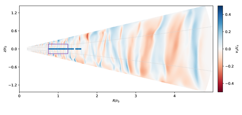
Figure 2: Same as Fig. 1, but now in natural (linear cylindrical) coordinates.

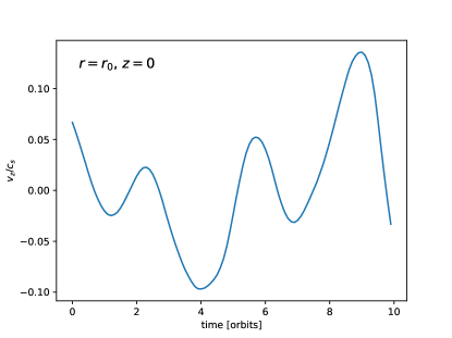
Figure 3: For the fiducial model shown in Figs. 1 and 2, the vertical gas velocity $v_{z}$ at $r=r_{0}$ and $z=0$ in units of the local isothermal sound speed as a function of time in units of orbits after the 300th orbit.

For these 20 orbits we now follow, as a post-processing step, the motion of $N=2000$ large dust particles that have been randomly placed between $0.75\,r_{0}$ and $1.6\,r_{0}$ radially, and between $-0.001\,r_{0}$ and $+0.001\,r_{0}$ vertically. The particle velocities are initialized as being equal to the local Kepler velocity. The particles all have the same $\mathrm{St}_{0}$, meaning that if they were placed at $r=r_{0}$ and $z=0$, they would have Stokes number $\mathrm{St}=\mathrm{St}_{0}$. At each time step, for each particle, we recompute $\mathrm{St}$ based on the local conditions, consistent with keeping the grain size constant. The equations of motion of the particles include the force of gravity as well as the friction with the gas. We implement the numerical integration of these equations in a Python program. The particles do not have dynamical feedback onto the gas, allowing the gas hydrodynamics to be precomputed, and the dust particle dynamics to be computed in post-processing mode.

Given that the particles, in spite their comparatively large size (of the order of $\sim$millimeter), are much smaller than the mean free path of the gas molecules, the friction force is the simple Epstein drag law. At each time step the local gas temperature, density and velocity are linearly interpolated in time and space from the precalculated 200 snapshots from the hydrodynamic simulation, using the RegularGridInterpolator function of the SciPy library.

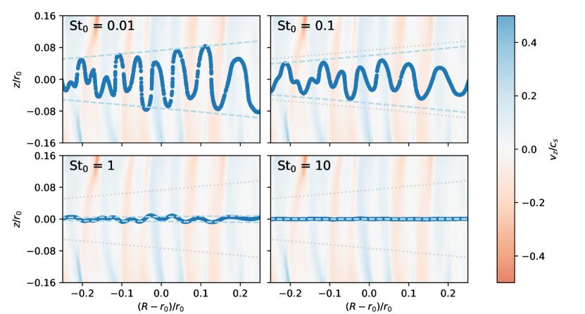
Figure 4: Snapshots of the location of the particles (blue dots) 2.5 orbits after they were inserted at the midplane into the fully developed VSI hydrodynamic model, for four values of $\mathrm{St}_{0}$. The coordinates are the cylindrical radius $R$ in units of, and relative to, $r_{0}$, and the cylindrical vertical height $z$ above the midplane in units of $r_{0}$. The background image shows the vertical gas velocity $v_{z}$, where blue is upward and red is downward, in the same color scale as in Fig. 1. The gray dotted lines show the gas pressure scale height for comparison. The lightblue dashed lines are the conveyor-belt estimate of the maximum vertical height of the dust particles, Eq. (2) with an upper cap at $z=h_{p}$ (which is why the dashed and dotted lines overlap for $\mathrm{St}_{0}=0.01$).

In Fig. 4 the results of the model are shown for $\mathrm{St}_{0}=0.01$, $\mathrm{St}_{0}=0.1$, $\mathrm{St}_{0}=1$, and $\mathrm{St}_{0}=10$, after 2.5 orbits at radius $r_{0}$. This short time is enough to achieve approximately the typical heights above and below the midplane that the particles acquire, and this does not change much in time after that. For $\mathrm{St}\gtrsim 1$, the conveyor-belt estimate of the height $z_{\mathrm{max}}$ above the midplane that the particles are stirred (Eq. 2) appears to be a reasonably good estimate, as can be seen by comparing the vertical locations of the particles with the light-blue dashed lines in the figure. For $\mathrm{St}=0.1$ it is not bad, but for smaller Stokes number the conveyor-belt esimate strongly overestimates the stirring-up height of the particles. This is because the VSI motions oscillate with a period of a few local Kepler orbits (see Fig. 3), which means that before the particles have arrived at their maximum possible elevation, they will be transported back down by the gas.

It is evident that the $\mathrm{St}_{0}=0.01$ particles are stirred up to one gas pressure scale height. This is entirely due to the VSI, and not due to any $\alpha$-diffusion, which is not included in the model. For $\mathrm{St}_{0}=0.1$, which is typically the highest Stokes number expected in dust coagulation models in the outer disk regions (Drazkowska et al., 2021), the dust particles are still stirred up to a substantial fraction of the gas pressure scale height. Even for $\mathrm{St}_{0}=1$ the particles get up to a height $z/R\sim 0.005$, which is about 7% of the gas pressure scale height, which is marginally consistent with the upper limit obtained for Oph 163131. If we go to $\mathrm{St}_{0}=10$, the particles remain close to the midplane, producing a thin layer well within the vertical geometric thinness of the observed dust layer of Oph 163131. However, as is shown in Section 3, it is unlikely that the particles in this dust layer have $\mathrm{St}_{0}\gtrsim 1$.

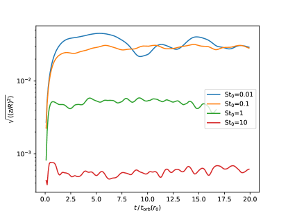
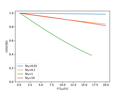
Figure 5: Mean values of the particles as a function of time since their insertion into the hydrodynamics model. Left: The root-mean-square of the $z/r$ ratio of the particles. Right: the mean of the radius to initial radius ratio ($r(t)/r(t=0)$), as a measure of how strongly the particles have radially drifted inward since the time of insertion. For the $\mathrm{St}_{0}=1$ case the computation was halted after 17 orbits, when the first particles left the inner orbit of the model.

To see this more quantitatively, we compute the root-mean-square of the $z/r$ ratio of the particles $\sqrt{\langle(z/r)^{2}\rangle}$ as a function of time since insertion. This is a measure of the vertical extent of the dust layer. The results are shown in Fig. 5-left. As can be seen, for $\mathrm{St}_{0}\geq 0.1$ the particles quickly reach a steady-state vertical extent, which is smaller for larger values of $\mathrm{St}_{0}$.

For $\mathrm{St}_{0}=1$ the radial drift of the particles becomes so fast that after 17 orbits the first particles leave the grid of the model at the inner edge. The calculation is then halted.

In general it should be noted that the rapid radial drift of large dust particles is a long-standing problem in the interpretation of millimeter wave observations of protoplanetary disks (Birnstiel et al., 2009). One explanation could be that the gas disks are so massive, that even millimeter particles in the outer regions of protoplanetary disks do not drift at excessive speeds (Powell et al., 2017). Another explanation is that radial drift of these particles is inhibited by dust trapping in one or more local pressure maxima (Pinilla et al., 2012). This would imply that the dust we observe with ALMA in the outer regions of protoplanetary disks ($r\gtrsim 20\,\mathrm{au}$) is either trapped in vortices or in rings. Both features are indeed observed with ALMA in numerous disks (e.g., van der Marel et al., 2013; Dong et al., 2018; ALMA-Partnership, 2015; Huang et al., 2018) and thus lend support to this picture. This means that the very flat dust midplane layers, if they consist of a series of concentric rings, could very well be made up of large dust particles, without experiencing the strong radial drift that the particles in our model undergo.

In principle this means that our models should be repeated for the case of disks with radial pressure bumps. However, since the origin of these pressure bumps is not yet clear, this would introduce a series of new and unconstrained model parameters. Also, a variety of additional phenomena could occur in these traps (e.g., Carrera et al., 2021; Lehmann & Lin, 2022). So for this paper we limit ourselves to disks without pressure traps.

2.3 Dynamics of dust modeled as a fluid

The dust motion can also be modeled directly within the hydrodynamics model. For this we employ the Fargo3D code (Benitez-Llambay & Masset, 2016), which has dust dynamics built in (Krapp & Benitez-Llambay, 2020). Like before, we assume a locally isothermal equation of state, maximizing the VSI activity. The dust is treated as a pressureless fluid, which feels friction with the gas. In the standard setup of Fargo3D, the gas feels the opposite force from the dust. However, to make the comparison with the results of Section 2.2, we switch this feedback off. It is known that for high metallicity $Z$ the VSI can be hampered simply by the mass of the dust (Schäfer et al., 2020; Lehmann & Lin, 2022), which would be one possible explanation for the razor-thin dust disks seen in ALMA. But in this section we assume that this effect is not taking place. The background viscosity is set to $\alpha=10^{-6}$.

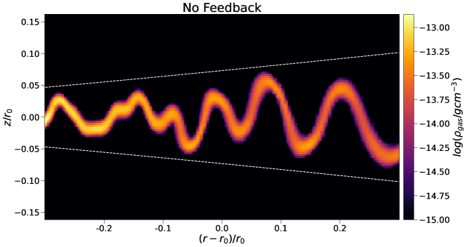
Figure 6: Spatial distribution of $\mathrm{St}_{0}=0.1$ dust in the hydrodynamic model in which both gas and dust are dynamically modeled as a fluid (Section 2.3). The white dashed lines mark one gas pressure scale height above/below the midplane.

The results for the case of $\mathrm{St}_{0}=0.1$ are shown in Fig. 6. The dust has been allowed to settle from the very beginning of the simulation over the entire modeling time. Throughout this time frame, the pattern of the dust remains corrugated. It is very comparable to the results of Section 2.2. The main difference is that in the dust-fluid approach the vertical width of the corrugated dust “layer” is thicker than in the particle approach of Section 2.2. This is due to numerical diffussivity.

Next, we put the result of this model into the RADMC-3D radiative transfer code and compute the images at an inclination of 84^∘, at a wavelength of $\lambda=1300\,\mu$m. The big grains were assumed to have a radius of 100 $\mu$m, and we used the corresponding opacity for them (see Appendix B). The results are shown in Fig. 7. The corrugated geometry of the dust “layer” is clearly seen. To stress the effect this has on identifying any potential radial gaps in the dust layer, we artificially added a gap between 87 au and 98 au and a slight reduction of the density between 3.5 au and 60 au according to the model of Villenave et al. (2022) for Oph 163131. This was done a-posteriori: the big-grain dust density from the hydrodynamic model of Fargo3D was multiplied by a radial function that reduces the density by a factor of 0.1 between 87-98 au and by 0.5 inward of 60 au. After that, it was inserted into the RADMC-3D code. As seen in Fig. 7, these features are not recognizable due to the strong vertical waves. These images are not convolved with the ALMA beam, as they merely serve as an illustration. For the case of Oph 163131, Villenave et al. (2022) show that the spatial resolution of ALMA easily suffices to rule out that the dust layer is as strongly corrugated as in Fig. 7.

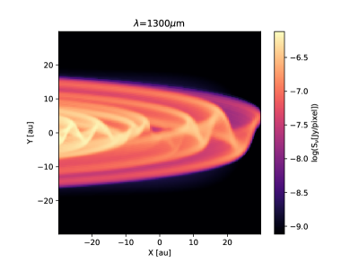
Figure 7: Synthetic image of the model of Section 2.3 at $\lambda=1.3$ mm at an inclination of 84^∘. Right panel is a zoom in (color-rescaled) of the left panel. The gap was added artificially to demonstrate how the VSI affects the observability of a gap. The images are idealized: no ALMA beam convolution is applied.

To highlight the difference between the VSI model and an equivalent model with a flat midplane layer, we show in Fig. 8 the comparison between these cases, for several inclinations. Again, no beam convolution is applied. Although the disk around Oph 163131 is used as a basis for these models, they are not meant to directly fit Oph 163131, but instead to illustrate the typical protoplanetary disk case (hence the different inclinations shown). It is clearly seen that at high inclinations, the VSI models look very different from the flat models, at scales easily resolvable with ALMA for objects at typical distances of about 100 pc. Also shown is the case where the big dust grains are vertically smeared out in a Gaussian layer with a vertical thickness half that of the gas ($h_{\mathrm{big}}=0.5\,h_{p}$). This mimicks the case when the vertical dust transport by the VSI would be treated as a vertical turbulent mixing instead of an actual advective transport. This case looks also substantially different from the VSI case. But it will depend on the distance of the object and the ALMA baselines whether they can be distinguished. The differences become less clear at lower inclinations, because the models only differ in vertical direction and are the same in radial direction.

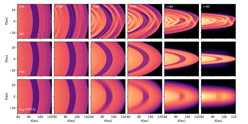
Figure 8: Comparison of the VSI model of Section 2.3 (top), a model with a flat dust layer (middle), and a model with a vertically extended dust layer with half the vertical thickness of the gas (bottom). Left-to-right: different inclinations. The synthetic observations are computed at $\lambda=1.3$ mm, and the images are centered 90 au offset from the star. No beam convolution is applied.

A caveat of these synthetic images of the VSI-stirred dust disk is that we have inserted only a single grain size. If we assume that the large grains follow a size distribution of a certain width, then the strong wiggles seen in the image get smeared out. The degree of smearing-out depends on the width of the size distribution. But it would not affect the conclusions of this paper.

This simulation confirms the results of Section 2.2 that even particles with a rather high Stokes number of $\mathrm{St}_{0}=0.1$ are stirred up to a substantial fraction of the gas pressure scale height, easily measureable with ALMA, and clearly in contrast with for instance the ALMA observations of Oph 163131.

As in the models of Section 2.2, the corrugated pattern of the dust layer is not static. It follows the time-dependent variations of the VSI velocity profile, where upward gas motions turn into downward motions and vice versa over time scales of a few local orbits. The model also confirms that the dust is not “vertically mixed” as in the simple vertical mixing-settling model of Dubrulle et al. (1995), Dullemond & Dominik (2004b) and Fromang & Nelson (2009). Instead, the corrugated structure of the dust is maintained, and the vertical extent is better described by the “conveyor-belt model” of Section 2.1.

2.4 Conclusion of this section

In this section we have shown that with a VSI operating in the disk, even particles with a Stokes number close to unity get stirred up to high elevations above the midplane, of the order of the gas pressure scale height. This is in conflict with ALMA observations of several protoplanetary disks, most strikingly the disk around Oph 163131 (Villenave et al., 2022).

However, for $\mathrm{St}_{0}\gg 1$ the midplane dust layer indeed becomes very geometrically thin, even in a disk in which the VSI is operating. So we need to rule out that these particles could have $\mathrm{St}_{0}\gg 1$, which is the topic of Section 3.

Once we ruled it out, we have to investigate how the VSI could be suppressed in the outer regions of protoplanetary disks. This is explored in Section 4.

3 The case against the midplane dust layer consisting of $\mathrm{St}\gg 1$ particles

As Section 2 showed, the geometric thinness of the midplane dust aggretate layers in protoplanetary disks can most easily be explained by particles that have $\mathrm{St}\gtrsim 1$, since they remain in a thin layer in spite of a possible VSI operating in the background. However, the dust rings seen in ALMA observations at $\lambda=1.3\,\mathrm{mm}$ tend to have optical depths larger than about $0.3$ at that wavelengths (Dullemond et al., 2018). For Oph 163131 in particular, Villenave et al. (2022) find with their radiative transfer modeling that the midplane dust layer is partially optically thick.

We demonstrate in this section that having both $\mathrm{St}\gtrsim 1$ and $\tau_{1.3\,\mathrm{mm}}\gtrsim 0.3$ requires a vertically integrated dust-to-gas ratio of at least $Z\gtrsim 0.08$, but likely $Z\gtrsim 0.16$. This value increases linearly with increasing $\mathrm{St}$ and $\tau_{1.3\,\mathrm{mm}}$.

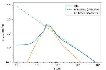
Figure 9: Dust opacity at $\lambda=1.3\,\mathrm{mm}$ as a function of grain size in units of cm² per gram of dust. Solid line: total opacity $\kappa_{1.3\,\mathrm{mm}}^{\mathrm{tot}}$; dashed line: effective scattering opacity $\kappa_{1.3\,\mathrm{mm}}^{\mathrm{scat,eff}}$; dotted line: Eq. (3) for $Q_{\lambda}=1.6$.

To arrive at this, we start with the dust opacity model described in Appendix B. In Fig. 9 the $\lambda=1.3\,\mathrm{mm}$ opacity as a function of grain size for this dust model is shown. Clearly the opacity $\kappa_{1.3\,\mathrm{mm}}$ is a strong function of the grain size $a$. It has a maximum value of 44.6 cm²/g at a grain size of $a=0.28\,\mathrm{mm}$. For $a\rightarrow 0$ the asymptotic value is $\kappa_{1.3\mathrm{mm}}\rightarrow$ 1.65 cm²/g. For $a\rightarrow\infty$ we can express $\kappa_{\lambda}$ in terms of the geometric opacity $\kappa_{\mathrm{geom}}$ defined as the geometric cross section $\pi a^{2}$ divided by the grain mass:

$$\kappa_{\lambda}=Q_{\lambda}\kappa_{\mathrm{geom}}=\frac{3}{4}\frac{Q_{\lambda}}{\rho_{s}a}\,,$$ (3)

where $\rho_{s}$ is the mean material density of the dust aggregate, and $Q_{\lambda}$ is the ratio of the opacity to the geometric opacity (van de Hulst, 1957 / 1981). For $a\gtrsim 1\,\mathrm{mm}$, Eq. (3) provides a good fit to the real opacity for a constant $Q_{\lambda}=1.6$. We note, however, that this equation can be used for all values of $a$, in which case $Q_{\lambda}$ will depend on $a$ and drop well below unity for $a\ll\lambda/2\pi$.

If we define the surface density of the big dust grains as $\Sigma_{\mathrm{big}}$, then the optical depth of the big dust grain layer becomes

$$\tau_{\lambda,\mathrm{big}}=\Sigma_{\mathrm{big}}\kappa_{\lambda}=\frac{3}{4}\frac{\Sigma_{\mathrm{big}}Q_{\lambda}}{\rho_{s}a}\,,$$ (4)

where $a$ is the radius of the big dust grains.

Next, let us compute, for the big dust grains, the Stokes number $\mathrm{St}$. For the outer regions of the protoplanetary disk we can assume that we are firmly in the Epstein friction regime, so that we can write (Birnstiel et al., 2010):

$$\mathrm{St}_{\mathrm{big}}=\frac{\pi\rho_{s}a}{2\Sigma_{\mathrm{g}}}\,,$$ (5)

where $\Sigma_{\mathrm{g}}$ is the surface density of the gas. We can combine Eqs. (4, 5) and eliminate $\rho_{s}a$, to obtain

$$Z_{\mathrm{big}}\equiv\frac{\Sigma_{\mathrm{big}}}{\Sigma_{\mathrm{g}}}=\frac{8}{3\pi}\frac{\mathrm{St}_{\mathrm{big}}\tau_{\lambda,\mathrm{big}}}{Q_{\lambda}}\,.$$ (6)

In the dust opacity model of Appendix B, for $\lambda=1.3\,\mathrm{mm}$, the maximum value of $Q_{\lambda}$ is 3.0, which is only reached in a narrow range of grain radii (see Fig. 9). For most values of $a$, $Q_{\lambda}\lesssim 1.6$. This means that if both $\mathrm{St}_{\mathrm{big}}\gtrsim 1$ and $\tau_{\lambda,\mathrm{big}}\gtrsim 0.3$, then Eq. (6) shows that $Z_{\mathrm{big}}\gtrsim 0.08\cdots 0.16$, i.e., the “metallicity” must be extremely high.

The question is then: is this a realistic scenario? Can the geometrically thin, but optically marginally thick ($\tau\gtrsim 0.3$) dust rings seen in many protoplanetary disks (and most strikingly seen in Oph 163131) be rings of dust particles with $\mathrm{St}_{\mathrm{big}}\gtrsim 1$ and $Z_{\mathrm{big}}\gtrsim 0.16$, or even $\mathrm{St}_{\mathrm{big}}\gg 1$ and $Z_{\mathrm{big}}\gg 1$, with a dynamics similar to the rings of Saturn? This scenario is completely different from the standard picture of dust dynamics in protoplanetary disks, which assume $\mathrm{St}_{\mathrm{big}}\ll 1$ and $Z_{\mathrm{big}}\ll 1$.

Although we cannot rule it out, we consider this scenario unlikely. The conditions derived in this section are the minimal conditions required. To be more comfortably within the limits, one would need $Z_{\mathrm{big}}/\mathrm{St}_{\mathrm{big}}\gg 0.16$, leading, for $\mathrm{St}_{\mathrm{big}}\gtrsim 1$, to very large values of $Z_{\mathrm{big}}$.

Using this constraint, we are then forced to consider mechanisms quenching the VSI entirely in order to understand the geometrical thinness of the dust rings. One way would be to load so much mass worth of dust in this midplane layer, that the gas is no longer able to lift it up from the midplane. As was shown by Lin (2019), Schäfer et al. (2020) and Lehmann & Lin (2022), the VSI is suppressed if the vertically integrated dust-to-gas ratio (“metallicity”) of the big grains exceeds about $Z\gtrsim 0.02\cdots 0.05$. Another way is to increase the cooling time scale, which is a natural consequence of grain growth (Fukuhara et al., 2021).

4 Inhibiting the VSI through depletion of small dust grains by grain growth

The VSI operates in disks which have, to good approximation, a locally isothermal equation of state. That is, at any given position $(r_{\mathrm{cyl}},z,\phi)$ in the disk the temperature of the gas $T_{g}(r_{\mathrm{cyl}},z,\phi)$ is fixed and does not vary in time. The justification for this is that in the outer regions of protoplanetary disks, the thermal household is determined by a balance between irradiation from the central star and thermal radiative cooling by the dust. The radiative cooling time scale $t^{\mathrm{rad}}_{\mathrm{cool}}$ for any perturbation of this equilibrium is short compared to the orbital time scale.

However, the cooling time is not completely negligibly small compared to the orbital time scale. As we shall show, only a moderate amount of dust coagulation is enough to increase the cooling time (or more accurately, the relaxation time; see Appendix D) beyond the limit where the VSI is stopped.

It was shown by Lin & Youdin (2015) that if the thermal relaxation is not fast enough, the vertical entropy gradient acts as a strongly stabilizing force against the VSI. They derive the following upper limit on the radiative relaxation time $t_{\mathrm{relax}}$:

$$t_{\mathrm{relax}}<\frac{|q|}{\gamma-1}\frac{1}{\Omega_{K}}\frac{h_{\mathrm{p}}}{r}\,,$$ (7)

where $q$ is the powerlaw index of the midplane temperature profile of the disk $T_{\mathrm{mid}}\propto r^{q}$, and $\gamma$ is the usual adiabatic index of the gas, which for the outer disk regions is $\gamma=5/3$ because the rotational and vibrational modes of H₂ are not excited at those temperatures. For our fiducial disk model (Appendix A) we have $q=-1/2$, and at $r=r_{0}=100\,\mathrm{au}$ we have $h_{\mathrm{p}}/r=0.0732$. So we obtain $t_{\mathrm{relax}}<0.055/\Omega_{K}$ as the upper limit on the thermal relaxation time for VSI to be operational.

Where in the protoplanetary disk this condition is met, and where not, was, among other things, explored by Pfeil & Klahr (2019). They found that the VSI is typically operational for radii $r_{\mathrm{cyl}}\gtrsim 10\,\mathrm{au}$, which are the regions of protoplanetary disks that have been resolved with ALMA, and where these geometrically thin dust layers are detected.

(Fukuhara et al., 2021) explore how dust evolution can change this, and they found that the coagulation of dust grains can increase the relaxation time scale and act against the VSI. A similar conclusion for the Zombie Vortex Instability was found by Barranco et al. (2018).

In this section we revisit this, and estimate $t_{\mathrm{relax}}$ in a simplified, yet robust way, including realistic dust opacities and the effect of dust depletion due to coagulation. We mimick the effect of coagulation by a simple conversion factor $\mathrm{X}\in[0,1]$ that says that a fraction $\mathrm{X}$ of the small grains has been converted into big grains that are not participating in the radiative cooling of the gas (these are probably the grains we observe with ALMA), while only a fraction $(1-\mathrm{X})$ of the small grains remain to radiatively cool the gas. In essence, we make the simplifying assumption that the dust consists of only two components: small submicron dust grains that are well-mixed with the gas, and are solely responsible for the radiative cooling, and big millimeter-size grains that tend to settle to the midplane unless they are stirred up by the gas.

4.1 Gas cooling via small dust grain emission

In the outer regions of a protoplanetary disk, the gas near the disk midplane is cold: $T_{\mathrm{mid}}\lesssim 70\,\mathrm{K}$. This means that the gas has very few emission lines, and no continuum, by which it can radiatively cool: typically only the rotational transitions of CO and its isotopologs, and maybe a few more complex molecules. Effectively this means that the gas is unable to radiatively cool by itself. It can only cool by transmitting its thermal energy to the available dust grains in the gas, which then can radiate away this energy.

In the midplane regions of the disk, the thermal coupling of gas and dust through collisions of gas molecules with the dust particles, is relatively efficient, though not perfect. The gas-dust thermal coupling time scale is estimated in Appendix F, but first we assume that the gas and dust thermally equilibrate fast enough that we can set $T_{g}=T_{\mathrm{small}}$, i.e., the gas temperature equals the small-grain dust temperature.

We ignore the effect of the large-dust-aggregates midplane layer, and focus only on the gas and the small dust grains floating in the gas. We assume that these small dust grains are well-mixed with the gas in vertical direction, so that the dust-to-gas ratio for these small dust grains is vertically constant.

Under these conditions, the fastest cooling happens in the optically thin regime, because the dust opacity is independent of the dust density (the amount of dust per unit volume of the disk).

The rate of thermal emission of the small dust grains per unit volume of the disk is:

$$q_{\mathrm{cool,\mathrm{small}}}=4\pi\rho_{d}\int_{0}^{\infty}\kappa^{\mathrm{abs}}_{\nu,\mathrm{small}}B_{\nu}(T_{\mathrm{small}})d\nu\,,$$ (8)

where $\rho_{d}$ is the volume mass density of the small dust grains, $\kappa^{\mathrm{abs}}_{\nu,\mathrm{small}}$ is their absorption opacity as a function of frequency $\nu$, and $B_{\nu}(T_{\mathrm{small}})$ is the Planck function at the dust temperature $T_{\mathrm{small}}$. It is convenient to express this in terms of the Planck mean opacity $\kappa_{P}(T_{\mathrm{small}})$ defined as

$$\begin{split}\kappa_{P}(T_{\mathrm{small}})&=\frac{\int_{0}^{\infty}\kappa^{\mathrm{abs}}_{\nu,\mathrm{small}}B_{\nu}(T_{\mathrm{small}})d\nu}{\int_{0}^{\infty}B_{\nu}(T_{\mathrm{small}})d\nu}\\ &=\frac{\pi}{\sigma_{\mathrm{SB}}T_{\mathrm{small}}^{4}}\int_{0}^{\infty}\kappa^{\mathrm{abs}}_{\nu,\mathrm{small}}B_{\nu}(T_{\mathrm{small}})d\nu\,,\end{split}$$ (9)

with $\sigma_{\mathrm{SB}}$ the Stefan-Boltzmann constant. We can then express $q_{\mathrm{cool,\mathrm{small}}}$ as

$$q_{\mathrm{cool,\mathrm{small}}}=4\rho_{\mathrm{small}}\kappa_{P}(T_{\mathrm{small}})\,\sigma_{\mathrm{SB}}\,T_{\mathrm{small}}^{4}\,.$$ (10)

In Appendix C we give a convenient approximate expression for $\kappa_{P}(T_{\mathrm{small}})$.

The thermal energy in the dust per unit volume of the disk is:

$$e_{\mathrm{th,\mathrm{small}}}=c_{V,\mathrm{small}}\,\rho_{\mathrm{small}}\,\,T_{\mathrm{small}}\,,$$ (11)

with $c_{V,\mathrm{small}}$ the specific thermal heat capacity of the dust, $c_{V,\mathrm{small}}\lesssim 10^{7}\,\mathrm{erg}\,\mathrm{g}^{-1}\,\mathrm{K}^{-1}$ (Draine & Li, 2001). The thermal energy in the gas per unit volume of the disk is:

$$e_{\mathrm{th,g}}=c_{V,g}\,\rho_{g}\,T_{g}\,,$$ (12)

with the specific thermal heat capacity of the gas given by

$$c_{V,g}=\frac{k_{B}}{(\gamma-1)\mu m_{u}}\,,$$ (13)

where $k_{B}$ is the Boltzmann constant, $\mu\simeq 2.3$ is the mean molecular weight of the gas in units of the atomic unit mass $m_{u}$, and $\gamma$ is the ratio of specific heats. The total thermal energy density is the sum of the two

$$e_{\mathrm{th}}=e_{\mathrm{th,g}}+e_{\mathrm{th,\mathrm{small}}}\,.$$ (14)

For a small-grain dust-to-gas ratio smaller than or equal to 0.01 we can safely approximate this as $e_{\mathrm{th}}=e_{\mathrm{th,g}}$. The optically thin radiative cooling time is then

$$t_{\mathrm{cool,thin}}^{\mathrm{rad}}=\frac{e_{\mathrm{th,g}}}{q_{\mathrm{cool,\mathrm{small}}}}\,,$$ (15)

assuming $T_{\mathrm{small}}=T_{g}=T_{\mathrm{mid}}$. In the optically thin limit this then becomes

$$t_{\mathrm{cool,thin}}^{\mathrm{rad}}=\frac{c_{V,g}}{4\sigma_{\mathrm{SB}}\kappa_{P}(T)}\frac{\rho_{g}}{\rho_{\mathrm{small}}}\frac{1}{T^{3}}\,.$$ (16)

However, what we need for the analysis of the VSI is the relaxation time, which is shown in Appendix D, to be

$$t_{\mathrm{relax,thin}}^{\mathrm{rad}}=\frac{1}{4+b}\,t_{\mathrm{cool,thin}}^{\mathrm{rad}}\,,$$ (17)

where

$$b=\frac{d\ln\kappa_{P}(T)}{d\ln T}\simeq 1.7\,,$$ (18)

where the $1.7$ is valid for the opacity model of Eq. (29) of Appendix C.

So far we have not included optical depth effects, and have therefore considered the most VSI-friendly scenario. Optical depth effects can only increase the relaxation time, not shorten it. We are primarily interested in the regions that are spatially resolvable with ALMA, meaning we are interested in $r\gtrsim 10$ au. The optical depth of the disk to its own radiation is moderate to low in these outer regions. Optical depth effects are therefore not expected to play a large role in these regions. But it is not a major effort to include them. In Appendix E we discuss the relaxation time scale in the optically thick regime, and write it as $t_{\mathrm{cool,thick}}^{\mathrm{rad}}$ given by Eq. (36).

Finally, we have to account for the time it takes to transfer heat between the gas and the dust, $t_{\mathrm{dg}}$. This will play a big role for disks around bright stars such as Herbig Ae/Be stars, where it will be the limiting factor of the radiative the cooling. In Appendix F we give an expression for $t_{\mathrm{dg}}$.

We estimate the combined cooling time scale to be the sum of all three time scales:

$$t_{\mathrm{relax}}=t_{\mathrm{relax,thin}}^{\mathrm{rad}}+t_{\mathrm{relax,thick}}^{\mathrm{rad}}+t_{\mathrm{dg}}\,,$$ (19)

which gives a smooth transition between regions, and ensures that the limiting factor determines the actual relaxation time.

In Fig. 10 this relaxation time is shown for the fiducial disk model of Appendix A, for small-grain dust-to-gas ratios of $Z_{\mathrm{small}}=10^{-2}$ (no depletion, i.e., $\mathrm{X}=0$), for $Z_{\mathrm{small}}=10^{-3}$ (a factor of 10 depletion of small dust grains, i.e., $\mathrm{X}=0.9$), and for $Z_{\mathrm{small}}=10^{-4}$ (a factor of 100 depletion of small dust grains, i.e., $\mathrm{X}=0.99$). The dotted lines represent $t_{\mathrm{relax,thin}}^{\mathrm{rad}}+t_{\mathrm{dg}}$, i.e., without optical depth effects.

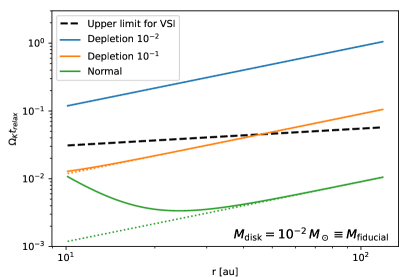
Figure 10: Relaxation time (Eq. 19) of the disk in units of the Kepler time $\Omega_{K}^{-1}$ for three small-grain dust-to-gas ratios: Normal ($Z_{\mathrm{small}}=10^{-2}$), depleted by a factor of $10^{-1}$ ($Z_{\mathrm{small}}=10^{-3}$) and depleted by a factor of $10^{-2}$ ($Z_{\mathrm{small}}=10^{-4}$). Dotted lines: optically thin approximation (Eq. 17). Solid lines: including optical depth effects. In dashed black: upper limit to the relaxation time (Eq. 7) for which VSI is operational is shown. The disk and stellar parameters are those of the star Oph 163131 (the fiducial model of Appendix A).

In Fig. 11 the same is shown for a 10 times lower disk mass, both in dust and in gas. Because of the lower optical depth, the solid curves are now closer to the optically thin estimates.

One can see that for both the fiducial model and for the 10$\times$ lower mass disk, $\Omega_{K}t_{\mathrm{relax}}$ is well below unity, justifying the locally isothermal appoximation for most applications. However, for the VSI to be operational, the relaxation time has to be below the limit given in Eq. (7), shown with the thick dashed line in Figs. 10 and 11.

For the fiducial model, with small-grain dust-to-gas ratio of $10^{-2}$, the thermal relaxation time scale is everywhere below this limit, meaning that the disk is prone to the VSI everywhere. However, if dust coagulation converts, say, 90% of the small grains into large dust aggregates (a depletion of $10^{-1}$, or $\mathrm{X}=0.9$), leading to a small-grain dust-to-gas ratio of $Z_{\mathrm{small}}=10^{-2}(1-\mathrm{X})=10^{-3}$, then the $\Omega_{K}t_{\mathrm{relax}}$ is above the threshold value for $r\gtrsim 50\;\mathrm{au}$. If coagulation converts 99% of the small grains (a depletion of $10^{-2}$, or $\mathrm{X}=0.99$), then the curve is everywhere well above the threshold, and the entire disk is VSI-stable.

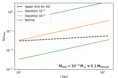
Figure 11: As Fig. 10, but now for 10x lower mass as the fiducial model, both in dust and gas.

If we redo our analysis for a brighter star, say a Herbig Ae star, then the disk will be warmer due to the stronger irradiation. This will lower the cooling times and thus make the disk more susceptible to the VSI. We show the resulting cooling time scales for a Herbig Ae star of $M=2.4\,M_{\odot}$ and $L=50\,L_{\odot}$, with otherwise the same disk parameters, in Fig. 12. Indeed, the cooling time for a normal dust-to-gas ratio is substantially shorter. A depletion of small grains of a factor of 10 is not sufficient, but a factor of 100 will, again, make the disk stable against the VSI in most of the disk.

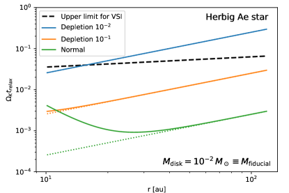
Figure 12: As Fig. 10, but now for a disk around a Herbig Ae star with $M=2.4\,M_{\odot}$ and $L=50\,L_{\odot}$.

A depletion of small dust grain by a factor of 10 or even 100 due to coagulation is not extreme. The fact that most protoplanetary disks look “fat” (geometrically vertically extended) in optical and near-infrared observations is not evidence of a lack of coagulation. In Appendix G we quantify this by computing the optical appearance of our fiducial disk at a wavelength of $\lambda=0.8\,\mu$m for various degrees of small-grain depletion. These images show that the typical appearance of the disk, with its two bright layers separated by a dark lane, is retained even at large degrees of depletion. The required amount of dust coagulation to inhibit the VSI is therefore within the observational constraints.

5 Discussion

5.1 Earlier work on the stirring of large grains by the VSI

The extreme effectiveness of the VSI to stir up even large dust aggregates to high elevations above the midplane is not a new result, and has been noted by several previous authors. Flock et al. (2017, 2020) presented detailed 3D radiation hydrodynamical models of protoplanetary disks with dust particle dynamics. They show that 0.1 mm and 1 mm dust grains achieve greater elevations above the midplane than expected from isotropic turbulence. Similar conclusions were also made by Lehmann & Lin (2022), who show the dependency of this effect on Stokes number $\mathrm{St}_{0}$ and vertically integrated dust-to-gas ratio $Z_{\mathrm{big}}$, although they focus on smaller values of the Stokes number than we explore in this paper. However, we put this into context with recent observational evidence of the extreme vertical geometrical thinness of the big-grain dust layers in (most?) protoplanetary disks.

5.2 Effect of dust traps

The fact that our models are for disks without dust traps limits the applicability of the results. If the large dust grains in the outer regions of protoplanetary disks remain at those large distances because they are trapped, then it is rather natural to get $Z_{\mathrm{big}}\gg 0.01$ in these traps because all the dust elsewhere will radially drift into these traps, enhancing $Z$ there. As argued by Lin (2019) and Lehmann & Lin (2022), this then could naturally push $Z_{\mathrm{big}}\gtrsim 0.02\cdots 0.05$ which, according to their simulations, strongly suppresses the VSI.

The fact that the upper limit of $Z_{\mathrm{big},VSI}$ for the VSI lies around the same value as the lower limit of $Z_{\mathrm{big},SI}$ for streaming instability (Carrera et al., 2017-04) leads to an interesting speculation. It was shown by Stammler et al. (2019), using an argument related to that of Section 3, that $Z_{\mathrm{big},SI}$ coincides with an optical depth at millimeter wavelengths of order unity, as appears to be observed in ALMA observations. They argue that dust traps attract more and more dust, until $Z_{\mathrm{big}}$ reaches $Z_{\mathrm{big},SI}$, at which point $Z_{\mathrm{big}}$ stabilizes: Any further dust added to the trap will be converted into planetesimals by the streaming instability, keeping $Z_{\mathrm{big}}=Z_{\mathrm{big},SI}$. If $Z_{\mathrm{big},SI}>Z_{\mathrm{big},VSI}$, then this self-regulating system naturally keeps the disk VSI-stable. This could be another natural explanation for the lack of VSI, but this requires more detailed study of the combined VSI+SI, as in Schäfer et al. (2020). So at this point, this is merely a speculative idea.

5.3 Effect of small but non-zero background turbulence

It was noted by Nelson et al. (2013) that the VSI is also damped if the viscosity parameter of the disk $\alpha\gtrsim 4\times 10^{-4}$, i.e., typically when the disk is turbulent due to the magnetorotational instability (MRI). While MRI turbulence will also stir up large grains away from the midplane, it is far less effective than the VSI. And so, somewhat paradoxically, the existence of weak, but no-zero, turbulence might, by inhibiting the VSI, allow large grains to settle to a thinner layer than is the case for a non-turbulent disk.

5.4 3D effects

Since our models are 2D in $(r,z)$, we cannot treat any potential non-axisymmetric modes, such as the formation of long-lived vortices (Lehmann & Lin, 2022). The main effect of the VSI acts in the $(r,z)$ directions, however, and is not dependent on the $\phi$-direction. Any 3D effects on the large-scale may affect the observational appearance of the disk, but will likely not affect our conclusion that the flat disks seen with ALMA are incompatible with the VSI.

5.5 Small-scale modes

The VSI may operate on smaller scales than we can model with our global models, for example, via the parametric instability mechanism described by Cui & Latter (2022). This can have consequences for the dust dynamics and dust growth. If the VSI operates on the large scales as explored in this paper, the observational consequences will be dominated by these large-scale motions, even if smaller-scale motions are superposed on them. However, as shown in (Cui & Latter, 2022), the small-scale motions excited by the larger ones act as an energy sink to the large-scale motions. The long-term saturation state of the large-scale VSI modes may therefore depend on the very small-scale motions that require super-high spatial resolution to resolve. (Cui & Latter, 2022) cite a resolution of 300 grid cells per scale height, which is out of reach for global simulations. These considerations show that it remains to be explored to which degree the VSI or any other instabilities are inhibited if a protoplanetary disk is observed to have a very flat midplane dust layer, and what this means for the implied conditions in the disk.

5.6 Uncertainties in the thermal relaxation time

Our estimates of the thermal relaxation time suffer from some uncertainties. First, they are very sensitive to the disk temperature profile $T(r)$. This is because radiative cooling goes as $\propto T^{4}$. But in practice this sensitivity is not so severe, because any uncertainty in the irradiation $q_{\mathrm{heat}}\propto L_{*}$ of the disk only enters the temperature as $T\propto q_{\mathrm{heat}}^{1/4}\propto L_{*}^{1/4}$. It does show, however, that for disks around Herbig Ae stars the relaxation times are smaller than for T Tauri stars.

A much more critical uncertainty is the dust opacity at long wavelengths. The popular Bell & Lin (1994) opacity represents a relatively low estimate, lower than what we use in this paper. This opacity model was used by Lin & Youdin (2015) and Pfeil & Klahr (2019) for their relaxation time estimates, which leads to less favorable conditions for the VSI than our estimates. Malygin et al. (2017) use the opacity model of Semenov et al. (2003), which is, for $T_{\mathrm{mid}}<100$ K, very similar to that of Bell & Lin (1994). The factor of $\sim$1.5 difference can mostly by explained by the use of a different dust-to-gas ratio, so that the dust opacities are more or less the same. In contrast, Fukuhara et al. (2021) use a simple analytic opacity model (see Ivezic et al., 1997), which is higher than what we use in this paper, and leads to more favorable conditions for the VSI than our estimates (although this effect is limited by the dust-gas coupling time scale that becomes the limiting factor). The comparison of these opacities is shown in Fig. 14. The opacity at the far-infrared and submillimeter of the dust in protoplanetary disks is notoriously uncertain, and the real opacity is likely somewhere between these two extremes.

Another major uncertainty is the dust-to-gas ratio. In our analysis we kept this constant at a value of $Z=0.01$, although we allowed coagulation to convert the small grain population (responsible for the radiative cooling) into a big grain population (responsible for the dust observed with ALMA). However, these big grains can radially drift, leading to a reduction of the dust-to-gas ratio in the outer regions. However, since the big grains do not contribute to the cooling, this does not affect our analysis. What matters is only the small grain abundance $Z_{\mathrm{small}}$. Dust coagulation can reduce $Z_{\mathrm{small}}$. What subsequently happens to $Z_{\mathrm{big}}$ is irrelevant for the estimation of $t_{\mathrm{relax}}$.

5.7 Non-flat rings

It should be noted that there are observed protoplanetary disks for which one or more of the rings do not appear to be geometrically very thin. For instance, Doi & Kataoka (2021) conclude, after detailed radiative transfer modeling, that the inner dust ring of HD 163296 is, in fact, likely to be vertically extended to about a gas pressure scale height. One interpretation of this could be that in this ring the cooling rate is, in fact, not sufficiently reduced by grain growth, so that the VSI is operational. From Fig. 12 it can be seen that for a small-grain depletion somewhere around $3\times 10^{-2}$, the inner disk regions remain unstable to the VSI while the outer disk regions stabilize against the VSI, which might explain why the inner ring of HD 163296 is vertically more extended than the outer one. A similar point was made by Fukuhara et al. (2021). The disk of HD 163296 is fairly dim at those wavelengths (Garufi et al., 2022), which does seem to point to substantial small-grain depletion.

6 Conclusions

In this paper we show that the geometrically very thin midplane layers of dust observed in many protoplanetary disks, most strikingly shown in a recent paper by Villenave et al. (2022), are evidence that the VSI is not operational in these outer disk regions. Dust particles with dimensionless stopping times $\mathrm{St}\lesssim 1$ would be stirred up by the VSI to a substantial fraction of the gas pressure scale height, even for large particles with $\mathrm{St}\simeq 0.1-1$. Only for even larger particles, with $\mathrm{St}\gtrsim 1$, does the dust layer remain largely unaffected by the VSI. But we show that to have such a layer being marginally optically thick ($\tau\gtrsim 0.3$) at ALMA wavelengths, as seems to be the case for many such rings, this requires a vertically integrated dust-to-gas ratio $Z_{\mathrm{big}}\gtrsim 0.08\cdots 0.16$, which we consider an unlikely scenario.

Damping or inhibiting the VSI in the outer regions of a protoplanetary disk can be due to an enhanced vertically integrated dust-to-gas ratio of $Z_{\mathrm{big}}\gtrsim 0.02\cdots 0.04$, as shown by Lin (2019) and Lehmann & Lin (2022), or due to a modest background turbulence (Nelson et al., 2013).

We show that another possible explanation is that dust coagulation has converted more than 90% of the small grains in the disk into big grains (likely the ones that make up the midplane dust layer). In that case, the gas cannot cool fast enough through the thermal emission of the small grains, and the VSI is inhibited, as shown by Lin & Youdin (2015). Small-grain dust depletion of more than 90% by coagulation ($\mathrm{X}=0.9$) is reasonable during the life time of these disks (Tanaka et al., 2005; Dullemond & Dominik, 2005; Birnstiel et al., 2010), and remains consistent with the SEDs of these disks (Dullemond & Dominik, 2004a).

Our conjecture is thus that protoplanetary disks that show geometrically thin disks in ALMA observations are stable against the VSI.

Appendix A Fiducial disk model

To be able to make estimates of the numbers for this paper, we choose as standard star the star Oph 163131, for which we take the parameters from the paper Villenave et al. (2022): $M_{*}=1.2\,M_{\odot}$, $R_{*}=1.7\,R_{\odot}$, $T_{*}=4500\,\mathrm{K}$, which leads to $L_{*}\simeq L_{\odot}$. As an estimate of the disk midplane temperature we use a simple flaring disk estimate:

$$T_{\mathrm{mid}}(r)=\left(\frac{\tfrac{1}{2}\varphi L_{*}}{4\pi r^{2}\sigma_{\mathrm{SB}}}\right)^{1/4}\,,$$ (20)

where $\varphi$ is the flaring irradiation angle (radiative incidence angle), which we take, somewhat arbitrarily, as $\varphi=0.05$. Usually this value gives temperatures that are reasonably consistent with observational measurements. From this midplane temperature the gas pressure scale height $h_{P}(r)$ can be computed through $h_{p}=c_{s}/\Omega_{K}$, with $c_{s}=\sqrt{k_{B}T_{\mathrm{mid}}/\mu m_{u}}$ the isothermal sound speed and $\Omega_{K}=\sqrt{GM_{*}/r^{3}}$ the Kepler frequency. The disk is flaring with $d\ln(h_{p}/r)d\ln(r)=0.25$.

We choose as reference radius $r_{0}=100\,\mathrm{au}$. With the above parameters, the temperature at this reference radius is 16 K, and the gas pressure scale height is $h_{p}(r_{0})/r_{0}=0.0732$. The radial distribution of gas and dust mass are assumed to follow a powerlaw

$$\Sigma_{g}(r) = \Sigma_{g,100}\left(\frac{r}{100\,\mathrm{au}}\right)^{-1}\,,$$ (21)

$$\Sigma_{\mathrm{\mathrm{small}}}(r) = \Sigma_{\mathrm{small},100}\left(\frac{r}{100\,\mathrm{au}}\right)^{-1}\,,$$ (22)

$$\Sigma_{\mathrm{big}}(r) = \Sigma_{\mathrm{big},100}\left(\frac{r}{100\,\mathrm{au}}\right)^{-1}\,,$$ (23)

where $g$ stands for gas, $\mathrm{small}$ for small grains and $\mathrm{big}$ for big grains. The normalization factors $\Sigma_{x,100}$ can be expressed in terms of the disk mass

$$\begin{split}M_{x}&=2\pi\int_{r_{\mathrm{in}}}^{r_{\mathrm{out}}}\Sigma_{x}(r)r^{2}dr\,,\\ &=7\times 10^{-5}\,\Sigma_{x,100}\left(\frac{r_{\mathrm{out}}}{\mathrm{au}}-\frac{r_{\mathrm{in}}}{\mathrm{au}}\right)\;M_{\odot}\,.\end{split}$$ (24)

For the direct comparison to Oph 163131, we take $r_{\mathrm{in}}=10\,\mathrm{au}$, $r_{\mathrm{out}}=120\,\mathrm{au}$, for which we obtain

$$M_{x}=7.78\times 10^{-3}\,\Sigma_{x,100}\;M_{\odot}\,.$$ (25)

For the fiducial disk model we choose $M_{g}=0.01\,M_{\odot}$, i.e., $\Sigma_{g,100}=1.29\,\mathrm{g}/\mathrm{cm}^{2}$.

For the simulations of the VSI we take $r_{\mathrm{out}}=500\,\mathrm{au}$ (keeping $\Sigma_{g,100}$ fixed), to ensure that around $r=r_{0}$ there are no boundary effects.

The initial vertical structure of the gas at the start of the hydrodynamic simulation is set up as follows. We use the equilibrium state derived in Nelson et al. (2013) with $p=-2.25$ and $q=-0.5$ such that $\Sigma\propto 1/R$. The velocity field is seeded with noise with an amplitude of 1% local $c_{s}$ to kickstart the VSI.

Appendix B Dust opacity model

Both the small dust grains that are suspended in the gas and the large dust grains that make up the midplane layer seen by ALMA are assumed to consist of the same refractory material: 0.87 mass fraction of pyroxene with 70% magnesium, and 0.13 mass fraction of amorphous carbon. This is the DIANA standard mixture (Woitke et al., 2016). In addition we add a mantel of water ice such that the water ice contributes 20% of the total mass (Pätzold et al., 2016). This reduces the mass fractions of pyroxene and carbon to 0.696 and 0.104, respectively. We assume a porosity of $p=$0.25. The material density of a dust grain made up of this material is $\rho_{s}=1.48\,\mathrm{g/cm}^{3}$.

To compute the opacities we use the publicly available code optool (Dominik et al., 2021). We use the “Distribution of Hollow Spheres (DHS)” method (Min et al., 2005) with $f_{\mathrm{max}}=0.8$. The opacities for different grain sizes are shown in Fig. 13. Whereever we plot or use the scattering opacity, we use the effective scattering opacity given by

$$\kappa_{\nu}^{\mathrm{scat,eff}}=(1-g_{\nu})\,\kappa_{\nu}^{\mathrm{scat}}\,,$$ (26)

where $g_{\nu}$ is the scattering anisotropy coefficient. The factor $(1-g_{\nu})$ is a simple way to account for anisotropy (Min et al., 2009). This effective scattering opacity gives a better estimate of the importance of scattering compared to absorption, because it weighs strongly forward scattering ($g_{\nu}\rightarrow 1$) less than isotropic scattering ($g_{\nu}\rightarrow 0$).

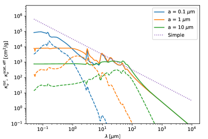
Figure 13: Dust grain opacity model used for this study. Shown here is the opacity as a function of wavelength for three grain sizes in units of cm² per gram of dust. Solid line: total effective opacity $\kappa_{\nu}^{\mathrm{tot}}=\kappa_{\nu}^{\mathrm{abs}}+\kappa_{\nu}^{\mathrm{scat,eff}}$; dashed line: effective scattering opacity $\kappa_{\nu}^{\mathrm{scat,eff}}=(1-g_{\nu})\kappa_{\nu}^{\mathrm{scat}}$. The dotted line represents the simple $\kappa_{\lambda}=3\pi/2\rho_{s}\lambda$ opacity model of Ivezic et al. (1997) in the vanishingly small grain size limit.

Also plotted in Fig. 13, for comparison, is a simple analytic dust opacity model proposed by Ivezic et al. (1997), in the limit of vanishingly small grain size. This model, and the version for finite grain sizes ($\kappa_{\lambda}=(\pi a^{2}/m)\min(1,2\pi a/\lambda)$, where $m$ is the grain mass and $a$ the grain radius), is often used in the literature because of its simplicity. It is also used in Fukuhara et al. (2021) to estimate the thermal relaxation time scale in protoplanetary disks.

Appendix C Rosseland and Planck mean opacity of the small dust grains

For the opacity model of Appendix B we compute here the Rosseland and Planck mean opacities. The Planck mean opacity was already defined in the main text (Eq. 9). The Rosseland mean opacity is defined as

$$\kappa_{R}(T_{\mathrm{small}})=\frac{\int_{0}^{\infty}(\partial B_{\nu}(T_{\mathrm{small}})/\partial T)d\nu}{\int_{0}^{\infty}(\partial B_{\nu}(T_{\mathrm{small}})/\partial T)/\kappa^{\mathrm{tot}}_{\nu,\mathrm{small}}d\nu}\,,$$ (27)

where

$$\kappa^{\mathrm{tot}}_{\nu,\mathrm{small}}=\kappa^{\mathrm{abs}}_{\nu,\mathrm{small}}+\kappa^{\mathrm{scat,eff}}_{\nu,\mathrm{small}}\,,$$ (28)

where the effective scattering opacity $\kappa^{\mathrm{scat,eff}}_{\nu,\mathrm{small}}$ is defined as in Eq. (26).

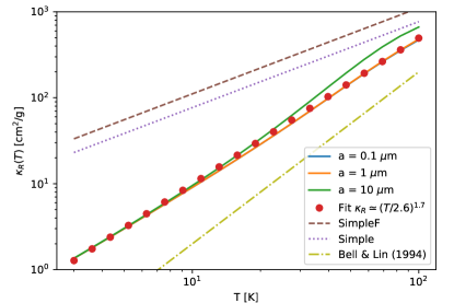
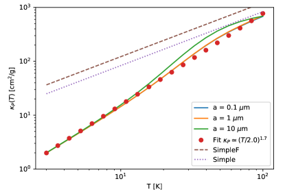
Figure 14: Small dust grain mean opacities as a function of temperature for three grain sizes. Left: Rosseland mean. Right: Planck mean. In the left panel the often-used opacity of Bell & Lin (1994) is plotted for comparison, which is used by Lin & Youdin (2015), Pfeil & Klahr (2019) and many other works. Malygin et al. (2017) use the dust opacity model of Semenov et al. (2003), which is, however, very similar to that of Bell & Lin (1994) in this temperature range. Also for comparison, the top two curves in each panel show the mean opacity for the simple $\kappa_{\lambda}=3\pi/2\rho_{s}\lambda$ small-grain opacity model used by Fukuhara et al. (2021), for our value of the material density $\rho_{s}=1.48\;\mathrm{g}\,\mathrm{cm}^{-3}$ (Simple) and their value of $\rho_{s}=1.00\;\mathrm{g}\,\mathrm{cm}^{-3}$ (SimpleF).

The resulting mean opacities are shown in Fig. 14. As one can see, for small enough grains and small enough temperatures, the Planck mean opacity of the dust can be well approximated for $T\lesssim 100\,\mathrm{K}$ and $a\lesssim 10\,\mu\mathrm{m}$ by the following fitting formula:

$$\kappa_{P}^{\mathrm{fit}}(T)=\left(\frac{T}{2.0\,\mathrm{K}}\right)^{1.7}\;\frac{\mathrm{cm}^{2}}{\mathrm{g}}\,,$$ (29)

where $\mathrm{g}$ is to be interpreted as gram of small-grain dust. The symbol $K$ is the unit of Kelvin. Likewise the Rosseland mean opacity can be approximated as

$$\kappa_{R}^{\mathrm{fit}}(T)=\left(\frac{T}{2.6\,\mathrm{K}}\right)^{1.7}\;\frac{\mathrm{cm}^{2}}{\mathrm{g}}\,,$$ (30)

For comparison, the dusty part of the Bell & Lin (1994) opacity is $\kappa_{R,\mathrm{BellLin}}(T)=2\times 10^{-2}\,(T/\mathrm{K})^{2}\;\mathrm{cm}^{2}/\mathrm{g}\simeq(T/7.07\,\mathrm{K})^{2}\;\mathrm{cm}^{2}/\mathrm{g}$, where we assume a dust-to-gas ratio of 0.01. The equivalent Planck-mean opacity for Bell & Lin would be $\kappa_{P,\mathrm{BellLin}}(T)=(T/4.58\,\mathrm{K})^{2}\;\mathrm{cm}^{2}/\mathrm{g}$. This means that our opacity model is more favorable to the onset of the VSI than the Bell & Lin opacity, implying that in our analysis we need to reduce the small-grain dust more strongly than the analysis done by Lin & Youdin (2015) and Pfeil & Klahr (2019) to suppress the VSI.

The primary reason why our opacity model exceeds that of Bell & Lin is the amorphous carbon mixed into the composition, which is responsible for the “antenna effect”, which strongly enhances the long-wavelength opacity. If the carbon would be, instead, in the form of organics, this effect would not be seen. The 25% porosity also increases the opacity a bit. If we use pure pyroxene without porosity, our opacity would exceed that of Bell & Lin by only 18%, which is well within the uncertainty of the dust-to-gas ratio we used to convert the Bell & Lin total opacity to a dust-only opacity. We refer to Woitke et al. (2016) for details on the role of carbon.

Appendix D Thermal relaxation time scale: The optically thin case

The thermal relaxation time scale is not identical to the cooling time scale. The radiative cooling time scale $t_{\mathrm{cool}}^{\mathrm{rad}}$ is given by Eq. (15), assuming $T_{\mathrm{small}}=T_{g}=T_{\mathrm{mid}}$, $e_{\mathrm{th}}=e_{\mathrm{th,g}}$, $\rho_{d}\ll\rho_{g}$, and $q_{\mathrm{cool}}=q_{\mathrm{cool,small}}$. In the optically thin limit this becomes Eq. (16). This is the time scale of cooling if the heating were to be suddenly switched off.

However, the condition of Lin & Youdin (2015) was derived for Newtonian cooling (linear in temperature), not for radiative cooling (proportional to $T^{4}$). This means that for the VSI we require the thermal relaxation time, which is the time scale on which a small deviation $\delta T$ from thermal equilibrium would exponentially decay (Malygin et al., 2017; Pfeil & Klahr, 2019). Local thermodynamic equilibrium implies $q_{\mathrm{cool}}=q_{\mathrm{heat}}$, where $q_{\mathrm{heat}}$ is, in our case, the irradiation of the disk by the star. The time-dependent equation for the thermal energy in an optically thin disk is then

$$\frac{de_{\mathrm{th,g}}(T)}{dt}=q_{\mathrm{heat}}-q_{\mathrm{cool}}(T)\,.$$ (31)

Defining the equilibrium temperature as $T_{0}$, we can add a small perturbation $\delta T$ and Taylor-expand Eq. (31) to first order:

$$\begin{split}\frac{e_{\mathrm{th,g}}}{T_{0}}\,\frac{d\delta T}{dt}\;\simeq&-\left(\frac{\partial q_{\mathrm{cool}}}{\partial T}\right)\delta T\,,\end{split}$$ (32)

where we used $e_{\mathrm{th,g}}\propto T$ (Eq. 12) and the condition for thermal equilibrium ($q_{\mathrm{cool}}(T_{0})=q_{\mathrm{heat}}$). The cooling rate, in the optically thin limit, is proportional to $q_{\mathrm{cool}}=q_{\mathrm{cool,\mathrm{small}}}\propto\kappa_{P}(T)\;T^{4}$. If the opacity follows a powerlaw $\kappa_{P}\propto T^{b}$, which in our case (see appendix C) would be $b=1.7$, then we can write

$$\left(\frac{\partial q_{\mathrm{cool,\mathrm{small}}}}{\partial T}\right)_{T=T_{0}}=(4+b)\;\frac{q_{\mathrm{cool,\mathrm{small}}}(T_{0})}{T_{0}}\,.$$ (33)

Eq. (32) can then be written as

$$\frac{d\delta T}{dt}\;\simeq-\frac{\delta T}{t^{\mathrm{rad}}_{\mathrm{relax,thin}}}\,,$$ (34)

with the thermal relaxation time given by

$$t^{\mathrm{rad}}_{\mathrm{relax,thin}}=\frac{1}{4+b}\;t^{\mathrm{rad}}_{\mathrm{cool,thin}}\,,$$ (35)

where $t^{\mathrm{rad}}_{\mathrm{cool,thin}}$ is given by Eq. (16).

Appendix E Thermal relaxation time scale: The optically thick case

For the optically thick case we follow Lin & Youdin (2015), who derived the relaxation time scale of a spatial radial temperature fluctuation $\delta T(r,t)\propto e^{ik_{x}x}$ with $x=r-r_{0}$ for the radius $r_{0}$ where the stability analysis is done, and $k_{x}$ is the spatial frequency of the wavelike fluctuation. The disk is assumed to be completely optically thick in vertical direction, and the radial radiative diffusion between the cooler and warmer part of the wave is assumed to dominate over the vertical radiative cooling. Lin & Youdin (2015) show that in that case, the relaxation time is given by

$$t^{\mathrm{rad}}_{\mathrm{relax,thick}}=\frac{1}{\eta k_{x}^{2}}\,,$$ (36)

with

$$\eta=\frac{16\sigma_{SB}T^{3}}{3\kappa_{R}(T)\rho_{\mathrm{small}}\rho_{g}c_{V,g}}\,.$$ (37)

The strongest optical depth effect (i.e., the largest value of $t^{\mathrm{rad}}_{\mathrm{relax,thick}}$) is found for the smallest realistic value of $k_{x}$, corresponding to the largest realistic length scale of the VSI mode. We set $k_{x}=2\pi/h_{p}$ as an estimate of this largest length scale. The optically thick and thin limits can be combined by adding the time scales together:

$$t^{\mathrm{rad}}_{\mathrm{relax}}=t^{\mathrm{rad}}_{\mathrm{relax,thin}}+t^{\mathrm{rad}}_{\mathrm{relax,thick}}\,.$$ (38)

Appendix F Thermal coupling of dust and gas

The rate of heat transfer between dust and gas is computed by assuming perfect thermal accomodation of a gas molecule after it hits a dust particle. This leads to a rate of heat transfer per unit surface area of a dust particle of

$$\tilde{q}_{\mathrm{dg}}=\rho_{g}\,\bar{C}_{H}\,(T_{g}-T_{\mathrm{small}})\,,$$ (39)

where $T_{g}$ is the gas temperature, $T_{\mathrm{small}}$ the temperature of the dust particle, $\rho_{g}$ the gas density, and $\bar{C}_{H}$ the heat exchange coefficient given by

$$\bar{C}_{H}=\frac{1}{\gamma-1}\,\sqrt{\frac{k_{B}T_{g}}{2\pi\mu m_{u}}}\,\frac{k_{B}}{\mu m_{u}}\,.$$ (40)

The rate of heat transfer per unit volume of the disk is then

$$q_{\mathrm{dg}}(T_{\mathrm{small}},T_{g})=\rho_{d}\,\rho_{g}\,\frac{s_{d}}{m_{d}}\,\bar{C}_{H}\,(T_{g}-T_{\mathrm{small}})\,,$$ (41)

with $s_{d}=4\pi a^{2}$ is the surface area of a spherical dust grain of radius $a$, which we set to $a=0.1\,\mu$m, and $m_{d}=\tfrac{4\pi}{3}\rho_{s}a^{3}$ is its mass, where we set $\rho_{s}=1.48\,\mathrm{g/cm}^{3}$ (see Appendix B). To compute the time scale for heat exchange between the gas and the dust, relative to the heat content of the gas, we compute

$$t_{\mathrm{dg}}=\frac{e_{\mathrm{th,g}}(T_{g})}{q_{\mathrm{dg}}(0,T_{g})}\,,$$ (42)

where $e_{\mathrm{th,g}}(T_{g})$ is the thermal energy in the gas, given by Eq. (12). In this equation we set $T_{\mathrm{small}}\rightarrow 0$ because we are computing a time scale (which, for $T_{\mathrm{small}}=T_{g}$ would be infinite), not the actual heat exchange.

We can plot the ratio of $t_{dg}/t^{\mathrm{rad}}_{\mathrm{relax,thin}}$, where $t^{\mathrm{rad}}_{\mathrm{relax,thin}}$ is given by Eq. (35). The result is shown in Fig. 15 for the fiducial model, the 10$\times$ less massive disk, and the Herbig Ae star model.

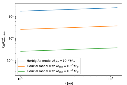
Figure 15: Ratio of the dust-gas thermal coupling time scale (Eq. 42) to the optically thin radiative relaxation time scale (Eq. 35) at the midplane of the fiducial disk as a function of radial coordinate in the disk, for a small-grain size of $0.1\,\mu$m. The three curves are the three models presented in this paper.

For the fiducial model with $M_{\mathrm{disk}}=10^{-2}M_{\odot}$, the value of $t_{dg}/t^{\mathrm{rad}}_{\mathrm{relax,thin}}$ is consistently below unity, meaning that the dust-gas thermal coupling is not the limiting factor of the cooling rate. However, for the less massive disk, the dust-gas coupling time scale starts to dominate, meaning that for such low mass disks the dust-gas coupling makes it easier to stabilize the disk against the VSI. For the Herbig Ae star model, the dust-gas coupling time scale dominates over the thermal relaxation time in the optically thin limit, but (as seen in Fig. 12), when optical depth effects start to play a role, the thermal relaxation time again dominates over the dust-gas thermal coupling time.

The inclusion of the dust-gas thermal coupling time is particularly important for the Herbig Ae star case. Without including it, the curves in Fig. 12 would be much lower (more favorable for the VSI).

Appendix G Optical appearance of a disk with strong depletion of small grains

A concern with the depletion of small grains to inhibit the VSI is that too much depletion would affect the appearance of the disk as seen in scattered light in the optical and near-infrared. At these wavelengths the stellar light scatters off the small dust grains in the surface layers of the disk, and the disk appears on the sky with a distinct “hamburger” shape, with light seen on two sides of a dark lane. If, however, the small grains are too strongly depleted, then this shape becomes flatter or disappears altogether. The question is: does a depletion factor of 0.1 or 0.01, required to inhibit the VSI, leave enough small grains in the disk to appear on the sky with this “hamburger” shape?

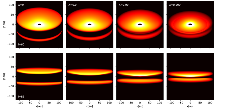
Figure 16: Appearance of the fiducial disk model at $\lambda=0.8\,\mu$m for four values of the coagulation parameter $\mathrm{X}=0$, 0.9, 0.99 and 0.999 (left to right), corresponding to a small-grain-depletion factor of 1, 0.1, 0.01 and 0.001. Top panels: inclination of $i=60$. Bottom panels: inclination of $i=85$. All images have the same logarithmic color scale spanning 3 factors of ten.

To find out, we run four radiative transfer models with RADMC-3D, all based on the fiducial disk model of appendix A, but with $\mathrm{X}=0$, 0.9, 0.99 and 0.999 (i.e., small-grain depletion factors of 1, 0.1, 0.01 and 0.001), and render images of them at $\lambda=0.8\,\mu$m and inclinations $i=60$ and $i=85$. The star is removed from the images. Both the small grains and the big grains are included in the model. For the big grain opacity at this wavelength, the extreme forward-peaked part of the scattering phase function is “chopped” within 10 degrees. This is a way to keep the Monte Carlo radiative transfer well-behaved without the need for an extremely high number of photon packages (see the manuals of RADMC-3D and of optool). The results are shown in Fig. 16.

It is clear that for all depletion factors the disk still appears in its characteristic shape with top and bottom bright layers separated by a dark lane. For stronger depletion of small grains the dark lane becomes narrower, as expected. For $\mathrm{X}=0.99$ and $\mathrm{X}=0.999$ the disk becomes vertically sufficiently optically thin that some of the starlight, after being scattered off the surface dust, reaches the midplane layer of large dust grains, which is visible in the images, albeit at very low brightness.

Of course, this also depends on the disk mass. And not all disks look alike. It therefore requires a case-by-case analysis. But overall we can conclude that the explanation of inhibiting the VSI by grain growth is not inconsistent with the typical appearance of protoplanetary disks at visual and near-infrared wavelengths.

Appendix H Comparison to a simple settling-mixing equilibrium

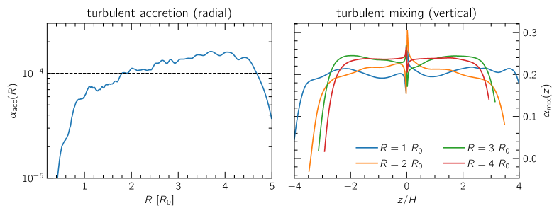
Figure 17: Measured turbulent radial-azimuthal viscosity and vertical mixing $\alpha$ coefficient, using the method of Stoll et al. (2017). Left: The viscous $\alpha$. Right: The vertical mixing $\alpha$ as a function of $z$ in units of the pressure scale height at four radii (in units of $r_{0}$).

It is instructive to compare the results of the particle motions to a simple vertical settling-mixing calculation such as those of Dubrulle et al. (1995), Dullemond & Dominik (2004b) and Fromang & Nelson (2009). The measured radial and vertical $\alpha$ of our model, using the method of Stoll et al. (2017), are shown in Fig. 17. It is evident that the turbulent motions of the VSI are highly anisotropic. The vertical turbulence parameter $\alpha_{\mathrm{mix}}$ is about 1700 times larger than the radial turbulence parameter $\alpha_{\mathrm{acc}}$. For the vertical mixing-settling calculation we use $\alpha_{\mathrm{mix}}$. According to Birnstiel et al. (2010), their Eq. (51), the geometric thickness $H_{\mathrm{big}}$ of the big grain dust layer can then be estimated as

$$H_{\mathrm{big}}\simeq h_{p}\min\left(1,\sqrt{\frac{\alpha_{\mathrm{mix}}}{\min(\mathrm{St},1/2)(1+\mathrm{St}^{2})}}\right)\,,$$ (43)

where the outer min() operator is because $H_{\mathrm{big}}$ is defined such that it cannot exceed $h_{p}$. For $\alpha_{\mathrm{mix}}\simeq 0.17$ and $\mathrm{St}\ll 1$, Eq. (43) reduces to $H_{\mathrm{big}}\simeq h_{p}\min(1,\alpha_{\mathrm{mix}}/\mathrm{St})$, and the dust will be almost as vertically extended as the gas ($H_{\mathrm{big}}\simeq h_{p}$), which is indeed what we find. For $\mathrm{St}\gg 1$, Eq. 43 reduces to $H_{\mathrm{big}}\simeq h_{p}\sqrt{2\alpha_{\mathrm{mix}}}/\mathrm{St}$. This matches the conveyor-belt estimate from Section 2.1 if we set $|v_{z,\mathrm{VSI}}|/c_{s}=\sqrt{2\alpha_{\mathrm{mix}}}$. However, from Fig. 3 we know that the typical values of $|v_{z,\mathrm{VSI}}|/c_{s}$ are of the order of 0.1, while the measured value of $\sqrt{2\alpha_{\mathrm{mix}}}$ from the simulation is about 0.58. It shows the limitations of these simple estimates.