Multidimensional Coherent Spectroscopy of Molecular Polaritons: Langevin Approach

Abstract

We present a microscopic theory for nonlinear optical spectroscopy of $N$ molecules in an optical cavity. A quantum Langevin analytical expression is derived for the time- and frequency-resolved signals accounting for arbitrary numbers of vibrational excitations. We identify clear signatures of the polariton-polaron interaction from multidimensional projections of the signal, e.g., pathways and timescales. Cooperative dynamics of cavity polaritons against intramolecular vibrations is revealed, along with a cross talk between long-range coherence and vibronic coupling that may lead to localization effects. Our results further characterize the polaritonic coherence and the population transfer that is slower.

Introduction.–Strong molecule-photon interaction has drawn considerable attention in recent study of molecular spectroscopy. New relaxation channels have been demonstrated to control fast electron dynamics and reaction activity [1, 2, 3, 4, 5, 6, 7, 8, 9]. Optical cavities create hybrid states between molecules and confined photons, known as polaritons [10, 11, 12, 13, 14]. Theoretically, this requires a substantial generalization of quantum electrodynamics (QED) into molecules containing many more degrees of freedom than atoms and qubits.

It has been demonstrated that light in a confined geometry can significantly alter the molecular absorption and emission signals [15, 16, 17]. The collective interaction between excitations of many molecules and photons is of fundamental importance, leading to interesting phenomena, e.g., superradiance and cooperative dynamics of polaritons [18, 19, 20, 21, 22, 23]. In contrast to atoms whereby superradiance and cavity polaritons are well understood, molecular polaritons are more complex in theory and experiments. This arises from the complicated couplings between electronic and nuclear degrees of freedom, which possess new challenges for optical spectroscopy. Recently the absorption and fluorescence spectra are described by Holstein-Tavis-Cummings model [24, 25]. Exact diagonalization of the full Hamiltonian was used to calculate the optical responses, by only taking a few vibrational excitations into account [11, 26]. Here we focus on the polaritonic relaxation pathways involving the population and coherence dynamics, which are however open issues. Ultrafast spectroscopic technique has been used to monitor the dynamics of vibrational polaritons [22, 27, 28]. Time- and- frequency-gated photon-coincidence counting was employed to monitor the many-body dynamics of cavity polaritons, making use of nonlinear interferometry [28, 29]. Polaritons reveal the effects of strongly modifying the energy harvesting and migration in chromophore aggregates, through novel control knobs not accessible by classical light [7, 13, 30, 31, 32]. Elaborate nonlinear optical measurements of molecular polaritons have demonstrated unusual correlation properties [33, 34, 35]. That calls for an extensive understanding of dark states with a high mode density [36, 37, 38, 39, 40, 41, 42], nonlinearities and multiexciton correlations [43, 44, 45, 46, 47].

Previous spectroscopic studies of cavity polaritons were mostly based on wave function methods including nonadiabatic nuclear dynamics [48, 49, 50], Redfield theory and quantum chemistry simulations of low excitations [51, 52, 53, 54, 55, 56]. Absorption and emission associated with multiple phonons and optically dark states depend on a strong polariton-polaron interaction, which raises a fundamental issue in cavity polaritons and however complicates the simulation of ultrafast spectroscopy.

In this Letter, we employ a quantum Langevin theory for time-frequency-resolved coherent spectroscopy of molecular polaritons. Analytical solution for multidimensional third-order spectroscopic signals is developed. The results reveal multiple channels and timescales of the cooperative relaxation of polaritons, and also the trade-off with dark states.

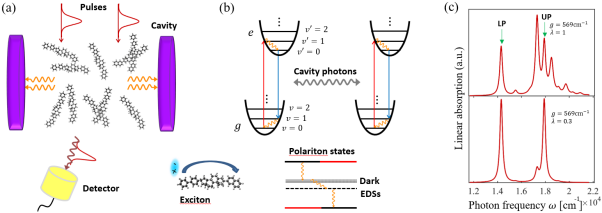
Figure 1: Schematic of time-resolved spectroscopy for molecular polaritons. (a) Emission signal is collected along a certain direction, once the molecules are excited by laser pulses. (b) Exciton-photon interaction in molecules in the presence of vibronic coupling attached to individual molecule. This results in the dark states and emitter dark states (EDSs) weakly interacting with cavity, apart from the upper and lower polariton modes; Rich timescales and channels of excited-state relaxation are thus expected. (c) Linear absorption of molecular polaritons with $10$ organic molecules in an optical cavity. The parameters are taken to be $\omega_{D}=16113$cm^-1, $\tilde{\delta}=\delta_{c}=0$, $\Gamma=20$cm^-1, $\gamma=1$cm^-1, $\gamma_{c}=0.9$cm^-1, $\omega_{\text{v}}=1200$cm^-1, typically from cyanine dyes [60].

Langevin model for polaritons.–Given $N$ identical molecules in an optical cavity, each has two energy surfaces corresponding to electronically ground and excited states, i.e., $|g_{j}\rangle$ and $|e_{j}\rangle\ (j=1,2,\cdots,N)$, respectively. Electronic excitations forming excitons couple to intramolecular vibrations and to cavity photons, as depicted in Fig.1(b), and are described by the Holstein-Tavis-Cummings Hamiltonian

$$\begin{split}H=\sum_{n=1}^{N}\left[\Delta_{n}\sigma_{n}^{+}\sigma_{n}^{-}+\omega_{\text{v}}b_{n}^{\dagger}b_{n}+g_{n}\big{(}\sigma_{n}^{+}a+\sigma_{n}^{-}a^{\dagger}\big{)}+\delta_{c}a^{\dagger}a\right]\end{split}$$ (1)

where $\Delta_{n}=\delta-\lambda\omega_{\text{v}}(b_{n}+b_{n}^{\dagger})$ and $\delta$ denotes the detuning between excitons and external pulse field. $[\sigma_{n}^{-},\sigma_{m}^{+}]=\sigma_{n}^{z}\delta_{nm}$. $\sigma_{n}^{+}=|e_{n}\rangle\langle g_{n}|$ and $\sigma_{n}^{-}=|g_{n}\rangle\langle e_{n}|$ are the respective raising and lowering operators for the excitons in the $n$th molecule. $b_{n}$ denotes the bosonic annihilation operator of the vibrational mode with a high frequency $\omega_{\text{v}}$, in the $n$th molecule. $a$ annihilates cavity photons. Each molecule has one high-frequency vibrational mode. In addition to the strong coupling to the single-longitudinal cavity mode, the molecules are subject to three temporally separated laser pulses whose electric fields $E_{j}(t-T_{j})e^{-iv_{j}(t-T_{j})}\ ;j=1,2,3$ described by $V(t)=\sum_{j=1}^{3}\sum_{n=1}^{N}V_{j,n}(t)+\text{h.c.}$ with $V_{j,n}(t)=-\sigma_{n}^{+}\Omega_{j}(t-T_{j})e^{-i(v_{j}-v_{3})t}e^{iv_{j}T_{j}}$ where $\Omega_{j}(t-T_{j})=\mu_{eg}E_{j}(t-T_{j})$ is the Rabi frequency with the $j$th pulse field and $\mu_{eg}$ is molecular dipole moment [57]. The full Hamiltionian is $H(t)=H+V(t)$, which yields the quantum Langevin equations (QLEs) for $\sigma_{n}^{-},a,b_{n}$.

We incorporate the polaron transform via the displacement operator $D_{n}=e^{\lambda(b_{n}-b_{n}^{\dagger})}$ into the QLE for the dressed operator $\tilde{\sigma}_{n}^{-}=\sigma_{n}^{-}D_{n}^{\dagger}$. This is to involve the exciton-vibration coupling to all orders, as it is normally moderate or strong. The QLEs for operators read a matrix form

$$\begin{split}\dot{\text{V}}=-\hat{\text{M}}\text{V}+\text{V}^{\text{in}}(t)+i\sum_{j=1}^{3}\Omega_{j}(t-T_{j})e^{iv_{j}T_{j}}e^{-i(v_{j}-v_{3})t}\text{W}_{\text{x}}\end{split}$$ (2)

after a lengthy algebra, where the term $\propto(b_{n}-b_{n}^{\dagger})=i\sqrt{2}p_{n}$ ($p_{n}$ is the dimensionless momentum of nuclear) has been dropped due to the nuclear velocity much lower than electrons [59]. The vector $\text{V}=[\tilde{\sigma}_{1}^{-},\tilde{\sigma}_{2}^{-},\cdots,\tilde{\sigma}_{N}^{-},a]^{\text{T}}$ involves $N+1$ components, and $\text{W}_{\text{x}}=[(2n_{1}-1)D_{1}^{\dagger},\cdots,(2n_{1}-1)D_{N}^{\dagger},0]^{\text{T}}$, $n_{l}=\tilde{\sigma}_{l}^{+}\tilde{\sigma}_{l}^{-}$. $\text{V}^{\text{in}}(t)=[\sqrt{2\gamma}\tilde{\sigma}_{1}^{-,\text{in}}(t),\cdots,\sqrt{2\gamma}\tilde{\sigma}_{N}^{-,\text{in}}(t),\sqrt{2\gamma_{c}}a^{\text{in}}(t)]^{\text{T}}$ groups the noise operators originated from exciton decay and cavity leakage. The matrix $\hat{\text{M}}$ in Eq.(2) reads

$$\begin{split}\hat{\text{M}}=\begin{pmatrix}i\tilde{\delta}+\gamma&0&\cdots&0&ig\sigma_{1}^{z}D_{1}^{\dagger}\\ 0&i\tilde{\delta}+\gamma&\cdots&0&ig\sigma_{2}^{z}D_{2}^{\dagger}\\ \vdots&\vdots&{}&\vdots&\vdots\\ 0&0&\cdots&i\tilde{\delta}+\gamma&ig\sigma_{N}^{z}D_{N}^{\dagger}\\ igD_{1}&igD_{2}&\cdots&igD_{N}&i\delta_{c}+\gamma_{c}\end{pmatrix}.\end{split}$$ (3)

We solve for the vibration dynamics: $b_{n}(t)\approx e^{-(i\omega_{\text{v}}+\Gamma)t}b_{n}(0)+\sqrt{2\Gamma}\int_{0}^{t}e^{-(i\omega_{\text{v}}+\Gamma)(t-t^{\prime})}b_{n}^{\text{in}}(t^{\prime})dt^{\prime}$, neglecting back influence from excitons, along the line of the stochastic Liouville equation [22, 55]. Eq.(2) represents the dynamics of molecular polaritons. Perturbation theory of the molecule-field interaction $V(t)$ will be used and we will calculate two-dimensional photon emission signals by placing the detectors off the cavity axis, shown in Fig.1(a). These signals are governed by multipoint correlation functions of the dipole operators and the corresponding Green’s functions, which are determined by the exact solution to the QLEs in Eq.(2).

The polariton emission.–We first present a general result for the emission spectrum of cavity polaritons. Subject to a probe pulse, Eq.(2) solves for the far-field dipolar radiation from molecules governed by the macroscopic polarization $P(t)=\mu_{eg}^{*}\sum_{i=1}^{N}\langle\sigma_{i;1}^{-}(t)\rangle$. We find the emission signal

$$\begin{split}P_{E}(\omega,T)=2i&|\mu_{eg}|^{2}\sum_{i=1}^{N}\sum_{l=1}^{N}\int_{-\infty}^{\infty}\text{d}t\int_{0}^{t}\text{d}\tau\ e^{i\omega t}E(\tau-T)\\[4.26773pt] &\ \ \times e^{-iv(\tau-T)}\langle G_{il}(t-\tau)n_{l}(\tau)D_{l}^{\dagger}(\tau)D_{i}(t)\rangle\end{split}$$ (4)

where $G(t)={\cal T}e^{-\int_{0}^{t}\hat{\text{M}}\text{d}t^{\prime}}$ is the free propagator without pulse actions. We note that, from the dressed excited-state populations $n_{l}(\tau)D_{l}^{\dagger}(\tau)$, the cavity polaritons of molecules undergo a dynamics against the local fluctuations from polaron effect. The polaron-induced localization as a result of dark states will compete with the cooperative dynamics of polaritons. These can be visualized from the emission signal, which will thus be a real-time monitoring of polariton dynamics through pulse shaping and grating. More advanced information will be elaborated by the multidimensional projections of the signals.

Linear absorption.–Assuming $\omega_{\text{v}}/T_{b}\gg 1$ that applies for organic molecules at room temperature, the vibrational correlation functions can be evaluated within vacuum state. Using Eq.(2), the absorption spectra reads $S_{A}(\omega)=\sum_{i,l=1}^{N}\sum_{m=0}^{\infty}S_{m}^{\lambda}\delta_{il}^{m}\text{Re}\left[{\cal G}_{il}(\omega-\xi_{m}^{*})\right]$ and $S_{m}^{\lambda}=e^{-\lambda^{2}}\lambda^{2m}/m!$ is the Franck-Condon factor. $\xi_{m}=m(\omega_{\text{v}}+i\Gamma)$ and ${\cal G}_{mn}(\Omega)=\int_{0}^{\infty}G_{mn}(t)e^{i\Omega t}dt$ is the Fourier component of the propagator $G(t)$. $S_{A}(\omega)$ resolves the lower polariton (LP) and upper polariton (UP) $\omega_{\text{LP}/\text{UP}}$, EDSs $\omega_{\text{D}}+m\omega_{\text{v}}$ decoupled from cavity photons while the dark states $\omega_{\text{D}}$ are not visible. To see these closely, we assume $\gamma=\gamma_{c},\ \tilde{\delta}=\delta_{c}=0$. The peak intensities can be thus found $S_{A}\left(\omega_{\mathrm{D}}+m\omega_{\mathrm{v}}\right)/S_{A}\left(\omega_{\mathrm{LP}/\mathrm{UP}}\right)\approx 2(\lambda^{2m}/m!)(\gamma_{\text{LP}/\text{UP}}/m\Gamma)$ and $S_{A}\left(\omega_{\mathrm{LP}/\mathrm{UP}}+m\omega_{\mathrm{v}}\right)/S_{A}\left(\omega_{\mathrm{LP}/\mathrm{UP}}\right)\approx 0$ when $N\gg 1$. The modes at $\omega_{\text{LP}/\text{UP}}+m\omega_{\text{v}}$ are hard to observe. Yet the EDSs at $\omega_{D}+m\omega_{\text{v}}$ may be of comparable intensities with polariton modes. Such spectral-line properties will be shown to be generally true in the time-resolved spectroscopic signals.

Fig.1(c,up) illustrates the absorption spectra where the LP and UP are prominent from the peaks at 14300cm^-1 and 17900cm^-1 seperated by $2g\sqrt{N}$. In between, we can observe an extra peak at $\omega_{D}+\omega_{\text{v}}$ supporting an EDS decoupled from cavity photons and the large oscillator strength owing to the density of states $\sim N$. Fig.1(c,down) shows that the EDSs are masked by the Rabi splitting for weaker vibronic coupling. This, as a benchmark to the strong-coupling case, elaborate the effect of vibronic coupling against the collective coupling to cavity photons. The localization nature of the EDSs is thus indicated from eroding the cooperativity between molecules, which will be elaborated in time-resolved spectroscopy.

2D polariton spectroscopy.–To have multidimensional projections of the emission signal, a sequential laser pulses have to interact with the molecular polaritons. As the first two pulses create excited-state populations and coherences $n_{l;2}(t)=\sigma_{l;1}^{+}(t)\sigma_{l;1}^{-}(t)$ where the 1st-order correction $\sigma_{l;1}^{\pm}$ is calculated from Eq.(2), we find

$$\begin{split}n_{l;2}(t)D_{l}^{\dagger}(t)=&\sum_{j=1}^{N}\sum_{j^{\prime}=1}^{N}\iint_{0}^{t}dt^{\prime\prime}dt^{\prime}{\cal E}_{1}^{*}(t^{\prime}-T_{1}){\cal E}_{2}(t^{\prime\prime}-T_{2})\\[4.26773pt] &\times G_{lj^{\prime}}^{*}(t-t^{\prime})G_{lj}(t-t^{\prime\prime})D_{j^{\prime}}(t^{\prime})D_{j}^{\dagger}(t^{\prime\prime})D_{l}^{\dagger}(t).\end{split}$$ (5)

The 3rd-order correction to the polarization follows Eq.(4) when the third pulse serves as probe. Given the time-ordered pulses, the transition pathways are selective resulting from the term cancellation. Inserting Eq.(5) into Eq.(4), we therefore proceed to the far-field polarization for the emission along the direction $\textbf{k}_{\text{I}}=-\textbf{k}_{1}+\textbf{k}_{2}+\textbf{k}_{3}$, i.e., $P(t)=\mu_{eg}^{*}\sum_{i=1}^{N}\langle\sigma_{i;3}^{-}(t)\rangle$ which yields

$$\begin{split}P(\omega)&=2i\sum_{i,l=1}^{N}\sum_{j,j^{\prime}=1}^{N}\iiiint_{0}^{\infty}dtd\tau dt^{\prime\prime}dt^{\prime}e^{i\omega t}{\cal E}_{3}(\tau-T_{3})\\[4.26773pt] &\ \ \times{\cal E}_{2}(t^{\prime\prime}-T_{2}){\cal E}_{1}^{*}(t^{\prime}-T_{1})\langle 0|G_{il}(t-\tau)G_{lj^{\prime}}^{*}(\tau-t^{\prime})\\[4.26773pt] &\ \ \times G_{lj}(\tau-t^{\prime\prime})D_{j^{\prime}}(t^{\prime})D_{j}^{\dagger}(t^{\prime\prime})D_{l}^{\dagger}(\tau)D_{i}(t)|0\rangle\end{split}$$ (6)

where the four-point correlation function of vibrations $\langle 0|D_{j^{\prime}}(t^{\prime})D_{j}^{\dagger}(t^{\prime\prime})D_{l}^{\dagger}(\tau)D_{i}(t)|0\rangle$ has to be evaluated explicitly. The 2D signal is usually detected via a reference beam as a local oscillator interfering with the emission. This leads to the heterodyne-detected signal $S_{\text{2D}}(\Omega_{3},T,\Omega_{1})=\text{Im}\int_{0}^{\infty}E_{\text{LO}}^{*}(\Omega_{3})P(\Omega_{3})e^{i\Omega_{1}\tau}d\tau$ with the Fourier transform against the 1st delay $\tau=T_{2}-T_{1}$, where $E_{\text{LO}}(\Omega_{3})$ is the Fourier component of the local oscillator field. In general, calculating the signal with Eq.(6) is hard due to the integrals over pulse shapes. The procedures can be simplified by invoking the impulsive approximation such that the pulse is shorter than the dephasing and solvent time scales. We further consider the few-photon cavity that draws much attention in recent experiments, and notice the vibronic coupling predominately accounted by the polarons. The most significant terms may be remained, allowing the approximation $g\sigma_{l}^{z}D_{l}^{\dagger}\approx gD_{l}^{\dagger}\approx g$ in Eq.(3). The higher-order corrections will be presented elsewhere. We obtain an analytical solution to the 2D polariton signal (2DPS), up to a real constant

$$\begin{split}&S(\Omega_{3},T,\Omega_{1})=ie^{i\phi}\sum_{i,l=1}^{N}\sum_{j,j^{\prime}=1}^{N}\sum_{p=1}^{N+1}\sum_{\{m\}=0}^{\infty}S_{\{m\}}^{\lambda}\delta_{j^{\prime}j}^{m_{1}}\delta_{il}^{m_{2}}\delta_{jl}^{m_{3}}\delta_{j^{\prime}l}^{m_{4}}\\[4.26773pt] &\ \times\delta_{ij}^{m_{5}}\delta_{ij^{\prime}}^{m_{6}}(-1)^{m_{3}+m_{6}}{\cal G}_{il}\left(\Omega_{3}+\xi_{m_{2}+m_{5}+m_{6}}\right)G_{lp}^{*}(T)G_{lj}(T)\\[4.26773pt] &\ \times e^{i\xi_{m_{3}+m_{4}+m_{5}+m_{6}}T}{\cal G}_{pj^{\prime}}^{*}\left(-\Omega_{1}-\xi_{m_{1}+m_{4}+m_{6}}\right)\end{split}$$ (7)

subsequently from Eq.(6), where $S_{\{m\}}^{\lambda}=\prod_{s=1}^{6}S_{m_{s}}^{\lambda}$ and $\phi$ encodes the global phase from the four classical pulses. Details of the derivation of the signals via QLEs are given in Supplemental Material [59].

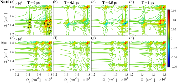
Figure 2: 2D time- and frequency-resolved signal for molecular polaritons where (up) $N=10$ organic molecules and (down) $N=1$ organic molecule. $T$ is varied, denoting the delay between the 2nd and the probe laser pulses. Horizontal and vertical axis are for absorption and emission frequencies, respectively. $\lambda=1$ and $g\sqrt{N}/\omega_{\text{v}}=1.5$. Other parameters are the same as Fig.1.

Simulations.–We have simulated the 2DPS to study polariton, exciton and polaron dynamics from the analytical solutions. We set $g\sqrt{N}/\omega_{\text{v}}=1.5$ for strong coupling.

The lower and upper rows in Fig.2 illustrate the 2DPS respectively for $N=1$ and $10$ molecules with fixed Rabi frequency $2g\sqrt{N}$. For 10 molecules in cavity, the signal reveals the real-time population transfer and coherence dynamics between polaritons and EDSs. The EDSs, however, cannot be resolved when one molecule coupled to cavity only. This is evident by the absence of the peaks at $\Omega_{1,3}=\omega_{D}\pm n\omega_{\text{v}}\ (n=0,1,2,...)$ in the lower row, compared with the upper row. The 2DPS for $N=1$ can monitor the states at $\omega_{\text{UP}}-integer\times\omega_{\text{v}}$ and their population transfer as well as coherence with the polariton states, as seen from the variation of the cross peaks, for example, at $(\Omega_{1}=\omega_{\text{UP}}-n\omega_{\text{v}},\Omega_{3}=\omega_{\text{UP}}-m\omega_{\text{v}}),m\neq n$ with the time delay $T$. We will present more details about the polariton dynamics against the EDSs next.

Fig.2(a) shows the 2D signal at $T=0$, from which the LP and UP states can be observed, evident by the two diagonal peaks at $\omega\pm g\sqrt{N}$. The cross peaks may result from the coherence and the polariton-polaron coupling, since energy and dephasing are not allowed at $T=0$. The former is due to the broadband nature of pump pulses while the latter is responsible for the change of phonon numbers associated with optical transitions. To have a closer look, we notice the states at $\Omega_{1}=14300,17300$ and $17900$cm^-1, after the absorbing energy from the pump pulse. These agree with the absorbance in Fig.1(c,up). The cross peaks imposing $\Omega_{1}-\Omega_{3}=integer\times\omega_{\text{v}}$ indicates the population of the EDSs which decouple from cavity photons and radiate phonons when emitting photons, evident by those at $(\Omega_{1}=17300\text{cm}^{-1},\Omega_{3}=14900\text{cm}^{-1})$ and $(\Omega_{1}=17300\text{cm}^{-1},\Omega_{3}=13700\text{cm}^{-1})$. The EDSs erode eroding molecular cooperativity and are highly degenerated, having the frequency $\omega_{D}\pm n\omega_{\text{v}};n=1,2,...$. The cross peaks with $\Omega_{1}-\Omega_{3}\neq integer\times\omega_{\text{v}}$ as circled in Fig.2(a), come from the coherences quantified by the off-diagonal elements of the density matrix. For instance, the one at $(\Omega_{1}=17900\text{cm}^{-1},\Omega_{3}=14900\text{cm}^{-1})$ resolves the coherence $\rho_{\omega_{D}-\omega_{\text{v}},\omega_{\text{UP}}}(T)$. The peaks associated with EDSs in both absorption spectrum and the 2D signal $S_{\text{2D}}(\Omega_{3},0,\Omega_{1})$ manifest in the steady state of molecular ensemble the role of local fluctuations that erodes the cooperative motion of exciton polaritons. This incredibly differs from previous studies showing the dynamical breakdown of the polariton-induced cooperativity of molecules by solvent motion which does not affect the polaritons significantly in the absorption spectrum, apart from the line broadening [22].

When the delay between the 2nd and probe pulses varies, Fig.2(b) show the fast decay of the coherence produced from the first two broadband pulses. This can be seen prominently from the decreasing intensities of the cross peaks with $\Omega_{1}-\Omega_{3}\neq integer\times\omega_{\text{v}}$, compared to Fig.2(a). From Fig.2(b), nevertheless, one can observe the cross peak at $(\Omega_{1}=17900\text{cm}^{-1},\Omega_{3}=14900\text{cm}^{-1})$ whose intensity increases after a rapid decay with the delay $T$. This describes the down-hill energy transfer from UP to the EDS $\omega=\omega_{D}-\omega_{\text{v}}=14900$cm^-1, following a fast dephasing. An energy transfer to LP is elucidated as well, from the growth of the cross peak at $(\Omega_{1}=17900\text{cm}^{-1},\Omega_{3}=14300\text{cm}^{-1})$. Similarly, the energy transfer pathway from the EDS $\omega=\omega_{D}+\omega_{\text{v}}=17300\text{cm}^{-1}$ to the LP can be observed within about 300fs. Observing the weak intensity along with a slow growth at the cross peaks $(\Omega_{1}=17900\text{cm}^{-1},\Omega_{3}=\omega_{D}-n\omega_{\text{v}})$ in Fig.2(b,c), the molecular system is slightly localized from the UP state within $\sim 500$fs because of the weak populations of EDSs. Within a longer timescale $T>500$fs, Fig.2(c,d) evidence that the energy flowing from UP and the state $\omega=\omega_{D}+\omega_{\text{v}}=17300\text{cm}^{-1}$ to the EDS $\omega=\omega_{D}-\omega_{\text{v}}=14900\text{cm}^{-1}$ dominates, leading to strong localization of the UP state. This can be neatly understood from the Fermi-Golden rule $\Gamma_{i\rightarrow f}=2\pi|\langle f|V|i\rangle|^{2}N_{i}D_{f}$ by noting a larger number of EDSs than polaritons. From the slice $\Omega_{1}=\omega_{D}+\omega_{\text{v}}=17300\text{cm}^{-1}$ in which the system can be pumped to the state at $\omega_{D}+\omega_{\text{v}}$ by the first two pulses, the system tends to be alternatively delocalized within a longer timescale $T>500$fs, seen from Fig.2(c,d) showing the strong peak intensity at LP state that indicates the population transferred considerably.

Moreover, one notes in Fig.2 that most of the cross peaks appear below the diagonal. This results from the low temperature assumed in our model, i.e., $\omega_{\text{v}}/T_{b}\gg 1$ so that the vibration modes are at vacuum initially before the pulse actions. During the first 250fs, the fast decay of the cross peak at $(\Omega_{1}=14300\text{cm}^{-1},\Omega_{3}=14900\text{cm}^{-1})$ monitors the dephasing of the coherence $\rho_{\omega_{D}-\omega_{\text{v}},\omega_{\text{LP}}}(T)$. The population transfer from the LP state to the EDS $\omega=\omega_{D}-\omega_{\text{v}}=14900\text{cm}^{-1}$ follows when the delay $T$ becomes longer, as indicated from the cross peak at $(\Omega_{1}=14300\text{cm}^{-1},\Omega_{3}=14900\text{cm}^{-1})$ that increases within about 750fs. Besides, the cross peak at $(\Omega_{1}=14300\text{cm}^{-1},\Omega_{3}=17900\text{cm}^{-1})$ shows up weakly within about 500fs, as depicted in Fig.2(c). A small portion of energy transferred from the LP state to the UP state is thus indicated. This may be attributed to the rapid energy exchange between the polariton and vibration modes, yielding a cascading migration of populations between two polariton modes within a short timescale. In longer timescales, such behavior is expected to deplete.

Relation to the pump-probe signal.–The pump-probe signal can be readily obtained by letting $T_{1}=T_{2}$ in Eq.(6) and accounting for the non-rephasing component. The signal reads $S_{\text{pp}}(\omega,T)=\text{Im}[E_{3}^{*}(\omega)P(\omega)]$ and some algebra gives

$$\begin{split}S_{\text{pp}}(\omega,T)=&\sum_{i,l=1}^{N}\sum_{j,j^{\prime}=1}^{N}\sum_{\{m\}=0}^{\infty}S_{\{m\}}^{\lambda}\delta_{il}^{m_{1}}\left(\delta_{j^{\prime}l}-\delta_{jl}\right)^{m_{2}}\left(\delta_{ij}-\delta_{ij^{\prime}}\right)^{m_{3}}\\[4.26773pt] &\times\text{Re}\left[{\cal G}_{il}\left(\omega+\xi_{m_{1}+m_{3}}\right)G_{lj^{\prime}}^{*}(T)G_{lj}(T)e^{i\xi_{m_{2}+m_{3}}T}\right]\end{split}$$ (8)

under the impulsive approximation. The broadband nature of the ultrashort pulses smears out the mode selectivity in the absorption of molecular polaritons, whereas the time grating makes the emission spectrally resolved. Similar as the 2DPS, the LP and UP modes separated by $2g\sqrt{N}$ as well as the EDSs at $\omega=\omega_{D}-m\omega_{\text{v}}$ can be resolved in $S_{\text{pp}}(\omega,T)$. As varying the time delay, the spectral-line intensity $S_{\text{pp}}(\omega_{\text{UP}/\text{LP}},T)$ shows a phase difference from the $S_{\text{pp}}(\omega_{\text{D}}-m\omega_{\text{v}},T)$, associated with different damping rates that are responsible for the incoherent channels of relaxations. The low spectral resolution with the absorption process, however, makes the pump-probe signal not capable of unveiling advanced information about the polariton dynamics and dark states, e.g., relaxation pathways and timescales. More details are given in SM [59].

Summary and outlook.–The microscopic theory of multidimensional spectroscopy for the molecular polaritons was developed, using the quantum Langevin equation capable of polariton-polaron interactions with high excitation number. Rich information about the fast-evolving dynamics of polaritons and dark states and their couplings can be readily visualized in the 2DPS, i.e., pathways and timescales. Our work manifests the ultrafast polariton-polaron interaction in molecules, resolving the EDSs against the polariton dynamics. This falls into a different category from the cavity QED for atoms, in which no relaxation between superradiant and subradiant states could be observed [61, 62, 63]. Understanding the collective nature of molecular polaritons is significant for the community to gain more details about the diverse phenomena afforded by the polaritons in complex materials. This knowledge may help in the design of cavity-coupled heterostructures in visible regime and in polariton chemistry.

Z.D.Z. gratefully acknowledges the support of ARPC-CityU new research initiative/infrastructure support from central (No. 9610505), the Early Career Scheme from Hong Kong Research Grants Council (No. 21302721) and the National Science Foundation of China (No. 12104380). D.L. gratefully acknowledges the support of the National Science Foundation of China, the Excellent Young Scientist Fund (No. 62022001). S.M. thanks the support of the National Science Foundation (No. CHE-1953045) and of the U.S. Department of Energy, Office of Science, Basic Energy Sciences, under Award No. DE-SC0022134.

References

- [1] A. Thomas, J. George, A. Shalabney, M. Dryzhakov, S. J. Varma, et al., Angew. Chem. Int. Ed. 55, 11462-11466 (2016)
- [2] J. Hutchison, T. Schwartz, C. Genet, E. Devaux and T. W. Ebbesen, Angew. Chem. 124, 1624-1628 (2012)
- [3] A. D. Dunkelberger, B. T. Spann, K. P. Fears, B. S. Simpkins and J. C. Owrutsky, Nat. Commun. 7, 13504-13513 (2016)
- [4] X. Li, A. Mandal and P. Huo, Nat. Commun. 12, 1315-1323 (2021)
- [5] F. Herrera and F. C. Spano, Phys. Rev. Lett. 116, 238301-238305 (2016)
- [6] L. Martinez-Martinez, R. Ribeiro, J. Campos-Gonzalez-Angulo and J. Yuen-Zhou, ACS Photonics 5, 167-176 (2018)
- [7] D. M. Coles, N. Somaschi, P. Michetti, C. Clark, P. G. Lagoudakis, P. G. Savvidis and D. G. Lidzey, Nat. Mater. 13, 712-719 (2014)
- [8] M. Kowalewski, K. Bennett and S. Mukamel, J. Phys. Chem. Lett. 7, 2050-2054 (2016)
- [9] J. Galego, F. J. Garcia-Vidal and J. Feist, Nat. Commun. 7, 13841-13846 (2016)
- [10] S. Aberra Guebrou, C. Symonds, E. Homeyer, J. C. Plenet, Yu. N. Gartstein, V. M. Agranovich and J. Bellessa, Phys. Rev. Lett. 108, 066401-066405 (2012)
- [11] F. C. Spano, J. Chem. Phys. 142, 184707-184718 (2015)
- [12] A. Shalabney, J. George, J. Hutchison, G. Pupillo, C. Genet and T. W. Ebbesen, Nat. Commun. 6, 5981-5986 (2015)
- [13] J. Flick, M. Ruggenthaler, H. Appel and A. Rubio, Proc. Natl. Acad. Sci. U.S.A. 114, 3026-3034 (2017)
- [14] J. M. Raimond, M. Brune and S. Haroche, Rev. Mod. Phys. 73, 565-582 (2001)
- [15] D. Wang, et al., Nat. Phys. 15, 483-489 (2019)
- [16] E. Hulkko1, S. Pikker, V. Tiainen, R. H. Tichauer, G. Groenhof and J. J. Toppari, J. Chem. Phys. 154, 154303-154312 (2021)
- [17] K. Georgiou, R. Jayaprakash, A. Askitopoulos, D. M. Coles, P. G. Lagoudakis and D. G. Lidzey, ACS Photonics 5, 4343-4351 (2018)
- [18] M. Tavis and F. W. Cummings, Phys. Rev. 170, 379-384 (1968)
- [19] M. Gross and S. Haroche, Phys. Rep. 93, 301-396 (1982)
- [20] M. O. Scully and A. A. Svidzinsky, Science 325, 1510-1511 (2009)
- [21] F. C. Spano, J. R. Kuklinski and S. Mukamel, Phys. Rev. Lett. 65, 211-214 (1990)
- [22] Z. D. Zhang, K. Wang, Z. Yi, M. S. Zubairy, M. O. Scully and S. Mukamel, J. Phys. Chem. Lett. 10, 4448-4454 (2019)
- [23] F. J. Garcia-Vidal, J. Feist and J. del Pino, New J. Phys. 17, 053040-053050 (2015)
- [24] F. Herrera and F. C. Spano, Phys. Rev. Lett. 118, 223601-223606 (2017)
- [25] M. Reitz, C. Sommer and C. Genes, Phys. Rev. Lett. 122, 203602-203607 (2019)
- [26] F. C. Spano and C. Silva, Ann. Rev. Phys. Chem. 65, 477-500 (2014)
- [27] B. Xiang, et al., Proc. Natl. Acad. Sci. U.S.A. 115, 4845-4850 (2018)
- [28] K. E. Dorfman and S. Mukamel, Proc. Natl. Acad. Sci. U.S.A. 115, 1451-1456 (2018)
- [29] Z. D. Zhang, P. Saurabh, K. E. Dorfman, A. Debnath and S. Mukamel, J. Chem. Phys. 148, 074302-074314 (2018)
- [30] M. Kowalewski, K. Bennett and S. Mukamel, J. Phys. Chem. Lett. 7, 2050-2054 (2016)
- [31] Z. D. Zhang, T. Peng, X. Y. Nie, G. S. Agarwal and M. O. Scully, arXiv:2106.10988v2 [quant-ph]
- [32] T. W. Ebbesen, Acc. Chem. Res. 49, 2403-2412 (2016)
- [33] F. Herrera, B. Peropadre, L. A. Pachon, S. K. Saikin and A. Aspuru-Guzik, J. Phys. Chem. Lett. 5, 3708-3715 (2014)
- [34] B. Xiang, R. F. Ribeiro, Y. Li, A. D. Dunkelberger, B. B. Simpkins, J. Yuen-Zhou and W. Xiong, Sci. Adv. 5, eaax5196 (2019)
- [35] B. Xiang, J. Wang, Z. Yang and W. Xiong, Sci. Adv. 7, eabf6397 (2021)
- [36] Z. D. Zhang and S. Mukamel, Chem. Phys. Lett. 683, 653-657 (2017)
- [37] M. A. Zeb, P. G. Kirton and J. Keeling, ACS Photonics 5, 249-257 (2018)
- [38] J. Galego, F. J. Garcia-Vidal and J. Feist, Phys. Rev. X 5, 041022-041035 (2015)
- [39] J. Flick and P. Narang, Phys. Rev. Lett. 121, 113002-113007 (2018)
- [40] L. Lacombe, N. M. Hoffmann and N. T. Maitra, Phys. Rev. Lett. 123, 083201-083206 (2019)
- [41] A. Csehi, Á. Vibók, G. J. Halász and M. Kowalewski, Phys. Rev. A 100, 053421-053429 (2019)
- [42] M. Du and J. Yuen-Zhou, Phys. Rev. Lett. 128, 096001-096007 (2022)
- [43] P. Saurabh and S. Mukamel, J. Chem. Phys. 144, 124115-124120 (2016)
- [44] J. Gu, et al., Nat. Commun. 12, 2269-2275 (2021)
- [45] S. Mukamel, J. Chem. Phys. 145, 041102-041104 (2016)
- [46] J.-H. Zhong, et al., Nat. Commun. 11, 1464-1473 (2020)
- [47] V. M. Axt and S. Mukamel, Rev. Mod. Phys. 70, 145-174 (1998)
- [48] M. Kowalewski, K. Bennett and S. Mukamel, J. Chem. Phys. 144, 054309-054316 (2016)
- [49] J. Flick, H. Appel, M. Ruggenthaler and A. Rubio, J. Chem. Theory Comput. 13, 1616-1625 (2017)
- [50] M. Gudem and M. Kowalewski, J. Phys. Chem. A 125, 1142-1151 (2021)
- [51] H.-P. Breuer and F. Petruccione, The Theory of Open Quantum Systems (Oxford University Press, Oxford, 2002)
- [52] N. T. Phuc, J. Chem. Phys. 155, 014308-014313 (2021)
- [53] F. Herrera and F. C. Spano, Phys. Rev. A 95, 053867-053890 (2017)
- [54] R. Saez-Blazquez, J. Feist, E. Romero, A. I. Fernandez-Domínguez and F. J. García-Vidal, J. Phys. Chem. Lett. 10, 4252-4258 (2019)
- [55] Y. Tanimura, J. Phys. Soc. Jpn. 75, 082001-082039 (2006)
- [56] R. F. Ribeiro, et al., J. Phys. Chem. Lett. 9, 3766-3771 (2018)
- [57] We have adopted the Condon approximation that is independent of the nuclear coordinates [58].
- [58] S. Mukamel, Principles of Nonlinear Optical Spectroscopy (Oxford University Press, Oxford, 1999)
- [59] See Supplemental Material for a detailed description of 2D coherent signal with quantum Langevin equation.
- [60] C. A. Guarin, J. P. Villabona-Monsalve, R. López-Arteaga and J. Peon, J. Phys. Chem. B 117, 7352-7362 (2013)
- [61] D. Pavolini, A. Crubellier, P. Pillet, L. Cabaret and S. Liberman, Phys. Rev. Lett. 54, 1917-1920 (1985)
- [62] W. Guerin, M. O. Araujo and R. Kaiser, Phys. Rev. Lett. 116, 083601-083605 (2016)
- [63] R. E. Evans, et al., Science 362, 662-665 (2018)