Matching Map Recovery with an Unknown Number of Outliers
Arshak Minasyan* Tigran Galstyan Sona Hunanyan Arnak Dalalyan
CREST, ENSAE, IP Paris 5 av. Henry Le Chatelier 91764 Palaiseau arshak.minasyan@ensae.fr RAU, YerevaNN 20 Charents street 0025 Yerevan tigran@yerevann.com Yerevan State University 1 Alek Manukyan 0025 Yerevan hunan.sona@gmail.com CREST, ENSAE, IP Paris 5 av. Henry Le Chatelier 91764 Palaiseau arnak.dalalyan@ensae.fr
Abstract
We consider the problem of finding the matching map between two sets of -dimensional noisy feature-vectors. The distinctive feature of our setting is that we do not assume that all the vectors of the first set have their corresponding vector in the second set. If and are the sizes of these two sets, we assume that the matching map that should be recovered is defined on a subset of unknown cardinality . We show that, in the high-dimensional setting, if the signal-to-noise ratio is larger than , then the true matching map can be recovered with probability . Interestingly, this threshold does not depend on and is the same as the one obtained in prior work in the case of . The procedure for which the aforementioned property is proved is obtained by a data-driven selection among candidate mappings . Each minimizes the sum of squares of distances between two sets of size . The resulting optimization problem can be formulated as a minimum-cost flow problem, and thus solved efficiently. Finally, we report the results of numerical experiments on both synthetic and real-world data that illustrate our theoretical results and provide further insight into the properties of the algorithms studied in this work.
1 INTRODUCTION
The problem of finding the best matching between two point clouds has been extensively studied, both theoretically and experimentally. The matching problem arises in various applications, for instance in computer vision and natural language processing. In computer vision, finding the correspondence between two sets of local descriptors extracted from two images of the same scene is a well-known example of a matching problem. In natural language processing, in particular, in machine translation, the correspondence between vector representations of the same text in two different languages is another example of a matching problem. Clearly, in these problems, not all the points have their matching point and one can hardly know in advance how many points have their corresponding matching points. The goal of the present work is to focus on this setting and to gain a theoretical understanding of the statistical limitations of the matching problem.
To formulate the problem and to state the main result, let and be two sequences of feature vectors of sizes and such that . We assume that these sequences are noisy versions of some feature-vectors, i.e.,
| (1) |
where and are two sequences of deterministic vectors from , corresponding to the original feature-vectors. The noise components of and are two independent sequences of i.i.d. isotropic Gaussian random vectors. Formally,
| (2) |
where is the identity matrix of size . We assume that for some of cardinality , there exists an injective mapping such that holds for all . We call the observations and inliers, while the other vectors from the sequences and are considered to be outliers. The ultimate goal is to recover based on the observations and only.
Various versions of this problem have been studied in the literature. Collier and Dalalyan [2013, 2016] considered the outlier-free case with equal sizes of sequences and (i.e., and ), whereas Galstyan et al. [2022] investigated the case with outliers in one of the sequences only (i.e., and ). Other variations of the matching problem under Hamming loss have been studied by Wang et al. [2022], Chen et al. [2022b], Kunisky and Niles-Weed [2022]. These papers obtain minimax-optimal separation rates and, in most cases, despite the discrete nature of the matching problem, provide computationally tractable procedures to achieve these rates.
When is an arbitrary subset of , which is the setting we focus on in this work, one can wonder whether the minimax separation rate is the same as in the case of known . Since the absence of knowledge on brings additional combinatorial complexity to the problem, one can also wonder whether it is still possible to conciliate statistical optimality and computational tractability. We show in this work that the answers to these questions are affirmative.
To explain our result, let us introduce the quantity
| (3) |
which is the signal-to-noise ratio of the difference of a pair of feature-vectors. Clearly, for matching pairs this difference vanishes. Furthermore, if vanishes or is very small for a non-matching pair, then there is an identifiability issue and consistent recovery of underlying true matching is impossible. Therefore, a natural condition for making consistent recovery possible is to assume that the quantity
| (4) |
is bounded away from zero. A recovery procedure is considered to be good, if the threshold such that recovers with high probability as soon as is as small as possible. It was proved in [Collier and Dalalyan, 2016] that when , one can recover with probability for . Furthermore, it was proved that this threshold is minimax optimal, i.e., optimal in the family of all possible recovery procedures. This implies that there are two regimes. In the low dimensional regime , the separation rate is dimension independent. In contrast with this, the separation rate scales roughly as in the (moderately) high dimensional regime .
Let us set
| (5) |
The main contributions of this work are the following.
-
•
For any given , we show that the Least Sum of Squares (-LSS) procedure, based on maximizing profile likelihood among matching maps between two sets of size , can be efficiently computed using the minimum cost flow problem. We denote the matching obtained using -LSS by .
-
•
If the value turns out to be smaller than and , we prove that makes no mistake with probability .
-
•
We design a data-driven model selection algorithm that adaptively chooses such that with probability , we have and as soon as .
The last item above implies that our data-driven algorithm achieves the minimax separation rate. More surprisingly, this shows that there is no gap in statistical complexities between the problems of recovering matching maps in outlier-free and outliers-present-on-both-sides settings.
2 RELATED WORK
In statistical hypothesis testing, the separation rates became key objects for measuring the quality of statistical procedures, see the seminal papers [Burnashev, 1979, Ingster, 1982] as well as the monographs [Ingster and Suslina, 2003, Juditsky and Nemirovski, 2020]. Currently, this approach is widely adopted in machine learning literature [Xing et al., 2020, Wolfer and Kontorovich, 2020, Blanchard et al., 2018, Ramdas et al., 2016, Wei et al., 2019, Collier, 2012]. Beyond the classical setting of two hypotheses, it can also be applied to multiple testing frameworks, for instance, variable selection [Ndaoud and Tsybakov, 2020, Azaïs and de Castro, 2020, Comminges and Dalalyan, 2012, 2013] or the matching problem considered here.
In computer vision, feature matching is a well-studied problem. One of the main directions is to accelerate matching algorithms, based on fast approximate methods (see e.g. Malkov and Yashunin [2020], Wang et al. [2018], Harwood and Drummond [2016], Jiang et al. [2016]). Another direction is to improve the matching quality by considering alternative local descriptors [Rublee et al., 2011, Chen et al., 2010, Calonder et al., 2010] for given keypoints. The choice of keypoints is considered in Tian et al. [2020], Bai et al. [2020].
The minimum cost flow problem was first studied in the context of the Hungarian algorithm [Kuhn, 2012] and the assignment problem, which is a special case of minimum cost flow on bipartite graphs with all edges having unit capacity. Generalization of Hungarian algorithm for graphs with arbitrary edge costs guarantees time complexity, where is the number of nodes in the graph, is the number of edges and is the total flow sent through the graph. There have also been other algorithms with similar complexity guarantees [Fulkerson, 1961, Ahuja et al., 1992]. Since then many algorithms have been proposed for solving minimum cost flow problems in strongly polynomial time [Orlin et al., 1993, Orlin, 1993, 1996, Goldberg and Tarjan, 1989, Galil and Tardos, 1988] with the fastest runtime of around . Recent advances for solving MCF problems have been proposed in Goldberg et al. [2015] and Chen et al. [2022a]. The latter proposes an algorithm with an almost-linear computational time.
Permutation estimation and related problems have been recently investigated in different contexts such as statistical seriation [Flammarion et al., 2019, Giraud et al., 2021, Cai and Ma, 2022], noisy sorting [Mao et al., 2018], regression with shuffled data [Pananjady et al., 2017, Slawski and Ben-David, 2019], isotonic regression and matrices [Mao et al., 2020, Pananjady and Samworth, 2020, Ma et al., 2020], crowd labeling [Shah et al., 2021], recovery of general discrete structure [Gao and Zhang, 2019], and multitarget tracking [Chertkov et al., 2010, Kunisky and Niles-Weed, 2022].
3 MAIN THEORETICAL RESULT
This section contains the main theoretical contribution of the present work. In order to be able to recover and the matching map , the key ingredient we use is the maximization of the profile likelihood. This corresponds to looking for the least sum of squares (LSS) of errors over all injective mappings defined on a subset of of size . Formally, if we define
| (6) |
to be the set of all -matching maps, we can define the procedure -LSS as a solution to the optimization problem
| (7) |
where denotes the support of function . In the particular case of , the optimization above is conducted over all the injective mappings from to . This coincides with the LSS method from [Galstyan et al., 2022].
Let be the error of , that is
| (8) |
For some values of tuning parameters and , as well as for some , initialize and
-
1.
Compute and .
-
2.
Set .
-
3.
If or ,
-
then output .
-
4.
Otherwise, increase and go to Step 1.
In the sequel, we denote by the output of this procedure. Notice that we start with the value of , which in the absence of any information on the number of inliers might be set to . However, using a higher value of might considerably speed up the procedure and improve its quality.
For appropriately chosen values of and , as stated in the next theorem, the described procedure outputs the correct values of and with high probability.
Theorem 1.
Let and be defined by (5). If , then the output of the model selection algorithm with parameters satisfies .
Since the condition on the separation distance compared to the case of known is different by only a slightly larger constant, from the perspective of statistical accuracy, the case of unknown is not more challenging than that of the known .
In the sequel, without much loss of generality, we assume that the sizes of and are equal, i.e., . Indeed, in the case, one can add points arbitrarily far from the rest of the points to the smaller set obtaining equal size sets and .
Notice that in the optimization problem (7) the domain of is a finite set of injective functions. For a given value of , the number of such functions is making thus an exhaustive search computationally infeasible. Instead, we show in Section 5 that the optimization problem formulated in (7) can indeed be solved efficiently with complexity , where the notation hides polylogarithmic factors, i.e., up to polylogarithmic factors, the computational cost is of order .
4 INTERMEDIATE RESULTS AND PROOF OF THEOREM 1
This section is devoted to the proof of our main result. Along the way, we establish some intermediate results which are of interest on their own. The proofs of some technical lemmas are deferred to Appendix A.
4.1 Sub-mapping Recovery by LSS for
The first question we address in this section is under which conditions the LSS estimator from (7) recovers correct matches. Of course, the only way of correctly estimating the true matching is to choose . However, it turns out that even if we overestimate the number of outliers and choose a value which is smaller than the true value , with high probability the -LSS estimator makes no wrong matches. Naturally, this result, stated in the next theorem, is valid under the condition that the relative signal-to-noise ratio of all incorrect pairs of original features is larger than some threshold.
Theorem 2 (Quality of -LSS when ).
Let for defined by (7), and
| (9) |
If and the signal-to-noise ratio satisfies the condition then, with probability at least , the support of the estimator is included in and coincides with on the set . Formally,
| (10) |
Proof of Theorem 2.
Note that the random vectors
| (11) |
are standard Gaussian and define the following quantities
| (14) |
For the ease of notation, for any matching map we also define as follows
| (15) |
We start with two auxiliary lemmas that will be used in other proofs as well. The proofs of these lemmas are deferred to the appendix.
Lemma 1.
Let be any matching map that can not be obtained as a restriction of on a subset of . Let be an arbitrary set satisfying and and let be the restriction of to . On the event , we have
| (16) |
Let be any matching map from that is not a restriction of . Since , there exists necessarily a as in Lemma 1 such that . For this , we have . This implies that cannot be a minimizer of over . As a consequence, on , any minimizer of over is a restriction of . Therefore, on , we have and . It remains to prove that .
Lemma 2.
Let with defined as in (14). Then, for every , is upper bounded by
| (17) |
We apply Lemma 2 with to show that . Clearly, a sufficient condition for the latter is
| (18) |
This system is equivalent to
| (19) |
Therefore, if the signal-to-noise ratio satisfies
| (20) |
we have . ∎
4.2 Matching Map Recovery for Unknown
If no information on is available, and the goal is to recover the entire mapping , one can proceed by model selection. More precisely, one can compute the collection of estimators and select one of those using a suitable criterion. To define the selection criterion proposed in this paper, let us remark that
| (21) |
is an increasing function. The increments of this function for are not large, since they essentially correspond to the squared norm of a pure noise vector distributed according to a scaled distribution with degrees of freedom. The main idea behind the criterion we propose below is that the increment of at is significantly larger than the previous ones and the gap is of order . Therefore, if is larger than the deviations of the distribution, we are able to detect the value of and to estimate the true matching.
Based on these considerations, for any tolerance level , we set and define the estimator111We use the convention
| (22) | ||||
| (23) |
with as in (9).
Theorem 3 (Model selection accuracy).
Let . If , then it holds that . Therefore, is an upper bound on the separation distance in the case of unknown .
A remarkable feature put forward by this result is that a data-driven selection of based on the increments of the test statistics leads to the recovery of , with high probability, under the same constraint on the separation rate as in the case of known . It is however important to underline that this criterion requires the knowledge of the noise level. Therefore, from the point of view of statistical accuracy, the case of unknown is not more difficult than the case of known , provided the noise levels are known. It is also worth mentioning that our procedure requires only , not and separately.
Proof of Theorem 3.
The main parts of the proof will be done in the following two lemmas, the proofs of which are postponed to the appendix. For the known value of it is more convenient to work with the normalized version of test statistics , denoted by and defined by
| (24) |
Lemma 3.
On the event, , we have .
Lemma 4.
On the event, , for every , we have .
4.3 Matching Map Recovery for Unknown and Unknown Noise Level
In the previous subsection, we considered the case of unknown with known noise levels and . Notice that we do not need to estimate parameters separately, it is sufficient to estimate only their squared sum, which is denoted by . In the definition of , we use the value of in the threshold for . When both and are unknown, we first estimate and then plug it in the selection criterion of .
Thus, we define “candidate” estimators of
| (25) |
The rationale for this definition is that for small values of , contains only correct matches and, therefore, is merely a sum of independent random variables drawn from the distribution with degrees of freedom. Hence, after division by , we obtain an estimator of . However, from the perspective of testing the values of , we need to slightly overestimate the noise variance. This is done through the multiplication by the inflation factor .
We are now ready to proceed with the proof of our main result stated in Theorem 1.
Proof of Theorem 1.
We will provide the proof only in the high dimensional setting, that is we assume throughout the proof that . First, we show that for every the condition from is satisfied on an event of high probability. Second, we prove that for this condition is violated on the same event of high probability. Therefore, the combination of these two results concludes the proof.
Using the first part of the proof of Lemma 4, for all on the event , we have
| (26) | ||||
| (27) | ||||
| (28) |
Using the second part of the proof of Lemma 2, we can further upper bound the expression from the last display as follows
| (29) |
Now we show that for the relative difference of function at points and is large enough. Indeed, we have
| (30) | ||||
| (31) | ||||
| (32) |
where the first inequality follows from the definition of function , while second and third inequalities are consequences of the definitions introduced earlier in this section. Then, on the event we bound the quantities and from the last display along with using the condition on . One can now check that if then , which in turn implies
| (33) | ||||
| (34) |
Thus, we have shown that on the event our model selection procedure will select , i.e., . The last equality implies that . Moreover, in view of Theorem 2 on the same event we have . Finally, using Lemma 2, we get that the event occurs with probability at least . Therefore, the desired result follows. ∎
4.4 Lower Bounds
Theorem 2 and Theorem 3 imply that the minimax rate of separation in the problem of recovering is at most of the order of defined in (5). An interesting and natural question is whether this rate is optimal. In the literature, the lower bounds for similar models have been proved, see [Collier and Dalalyan, 2016, Theorem 2] for the case of and [Galstyan et al., 2022, Theorem 5] for the general rectangular case . Our model is more general222Indeed, it involves an additional (unknown) parameter . than those of these two references, the same lower bound applies to our model. Therefore, combining the results of Theorem 3 and [Collier and Dalalyan, 2016, Theorem 2] along with the fact that the separation distance has the same rate in both theorems implies that is the optimal separation rate.
5 COMPUTATIONAL ASPECTS AND NUMERICAL EXPERIMENTS
In this section, we address computational aspects of the optimization problem from (7). We show that it can be cast into a minimum cost flow problem. The latter is also known as an imperfect matching problem and, to the best of our knowledge, the fastest algorithm with complexity is proposed in [Goldberg et al., 2015]. We then report the results of numerical experiments conducted on both synthetic and real data and highlight their relation to the aforementioned theorems stated and proved in Sections 3 and 4, respectively. Our reproducible codes are provided in the supplementary material.
5.1 Relation to Minimum Cost Flow Problem
Let , for , be the squared distances between observed feature-vectors. Consider the following linear program
| minimize | (35) |
subject to satisfying
| (36) |
known as the minimum cost flow problem. Above, the notation means that for all , and similar convention is used for .
The formulation as an MCF problem is obtained by adding two auxiliary nodes to the graph, called source and sink (see Fig. 1). We are interested in the flow of the minimal cost, where the cost of each edge except those adjacent to source and sink is assigned from the distance matrix . The cost of the rest of the edges is equal to . The capacity that can be sent through each edge is equal to . The supply of source and sink are and , respectively. The solution of (35) given the constraints (36) provides the weights , from which the matching can be recovered. Indeed, if then and are matched. The last constraint in (36) implies that the matching size (number of that are equal to ) will be . Though the algorithm provided in [Goldberg et al., 2015] has the fastest known asymptotic complexity, the implementation of their algorithm is out of the scope of this paper. Therefore, in our experiments, we used SimpleMinCostFlow solver from OR-tools library [Perron and Furnon, 2022].
5.2 Numerical Experiments on Synthetic Data
In this part, we conducted several experiments on synthetic data to support our theoretical findings. In these experiments, we constructed two sets of sizes consisting of -dimensional data points. The underlying matching size was set to . In other words, in each point cloud, we had inliers and outliers. We also fixed the confidence level at , i.e., . The procedure for generating synthetic data was as follows. We set and chose an additional parameter used to control throughout the experiments. Then, each coordinate of and was independently sampled from a Gaussian distribution with mean and standard deviation . Additionally, for every , we incremented every coordinate of by , i.e., and, for every , we incremented every coordinate of by . This allows the outliers of each point cloud to be sufficiently far from each other, hence a pair of outliers is less likely to be confused as a pair of inliers. Notice also that such a choice of generating outliers fits within the conditions of Theorem 1. Finally, the sequences and were generated according to (1) with , for all . We measured the performance of our estimator by its precision, which is the number of correctly matched inliers divided by .
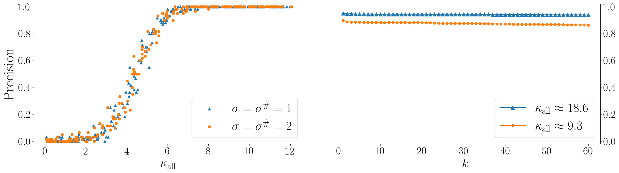
Let us now comment on the results obtained in Fig. 2. On the left plot, given that is large enough we observe that holds. Another interesting feature that can be inferred from Fig. 2 is that the precision is independent of the noise levels . This feature is consistent with Theorem 1 through the definition of which is independent of . The right plot upholds the findings of Theorem 2. Indeed, for some the support of will be included in the support of , plus, the values of and coincide on this support. Moreover, by plugging the values of this experiment into (9), we get , which means that the results proved in Theorems 1 and 2 hold whenever and , respectively. The results shown in Fig. 2 are the average values over independent trials of the same experiment.
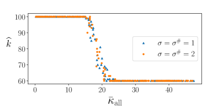
In the previous experiment, we focused on the case of known and noise levels. First, we consider the case of known noise levels and apply the estimator proposed in Section 4.2. In Fig. 3, we illustrate how the unknown value of is estimated for two different known noise levels. Namely, given that is “small” () all the pairs are considered as inliers and , as opposed to the experimental setup, where . However, given that the value of is large enough, the algorithm starts to differentiate inliers from outliers, hence we have starting from , which confirms the result of Theorem 3. Recall that the result of Theorem 3 holds whenever . Moreover, similar to the left plot of Fig. 2, the threshold after which the estimation becomes exact does not depend on noise levels. The results reported in Fig. 3 are the average values over independent trials of the same experiment.
Finally, we consider the case when no additional information is available neither about nor about , which corresponds to the most generic setting of Theorem 1. Recall the sequential procedure from Section 3 of estimating the triplet . In Fig. 4, we plot the dependencies of estimates of and on . There are several key features that are worth noticing. First, for small values of it is impossible to distinguish inliers from outliers, hence all points are treated as inliers and . As a consequence is overestimated. Second, for large enough values of both and are accurately estimated, therefore the precision of is (close to) . To make a link with Theorem 1 we also include the theoretical value of threshold in the plots.
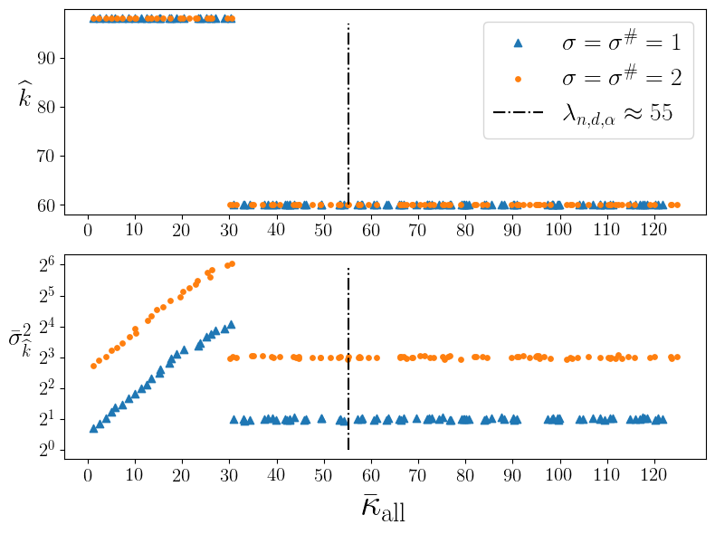
There are several takeaways that we would like to highlight. In the theoretical part, we proved that provided is large than the given threshold, it is possible to recover and to estimate . The threshold provided in theorems is rate optimal, however, it is not sharp. We observe that for different tasks the sharp threshold might differ up to a constant factor. For instance, in the case of known and we see that the threshold seems close to (see Fig. 2), while it is around in the more difficult setting of unknown and , as it is shown in Fig. 4. The setting of Fig. 3 is somewhat in between, since is assumed to be known but is unknown, hence the “change point” occurs around , which is between and . In practice, one could replace the theoretical quantiles of distribution with the empirical counterparts of the squared distances between matching pairs and for a given estimator .
5.3 Estimation of for Real Data
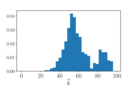
In what follows we carry out experiments on real data. In this experiment, we only focus on the estimation of the matching size in the setting of matching the keypoints (SIFT descriptors [Lowe, 2004]) of two different images of the same scene. The goal is to be able to match the same keypoints considering the noise present in the images, and not match the keypoints that are present in only one of the two images. We refer to Appendix B for more description and additional experiments in the keypoint matching problem.
Experiments on real data were conducted using IMC-PT 2020 dataset [Jin et al., 2020] consisting of 16 scenes with corresponding image sets and 3D point clouds. We used images from the “Reichstag” scene to illustrate how the procedure from Section 4.3 can be used to estimate the matching size. To construct the dataset, we randomly chose distinct image pairs of the same scene. Then, a scene point cloud is used to obtain pseudo-ground-truth matching between keypoints on different images of the same scene. Using these pseudo-ground-truth matching keypoints we then choose keypoints that are present in both images and add to each of them outlier keypoints. Hence, we have with and -dimensional SIFT descriptors. Notice that in the case of images, no information on and is available. Moreover, noise levels might not be homoscedastic. In Fig. 5, we present the histogram of the estimated value and observe that the procedure described in Section 4.3 provides a reasonably good estimate of .
Recall that at each iteration of estimating we solve an MCF problem, which can be computationally costly given the sample sizes are large. However, there are several aspects where we can speed up this procedure. First, using the Greedy algorithm to match the feature vectors (as done in OpenCV) will allow us to compute only one distance per iteration instead of solving MCF from scratch. Second, the stepsize from the second step of the procedure from Section 4.3 can be increased by considering the difference , then with a proper adjustment to the threshold, we will obtain a times speedup in the number of iterations.
5.4 Experiments on Biomedical Data
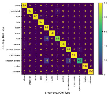
First, we tested our estimator from (7) in the setting of [Chen et al., 2022b][Sec. 5.1]. The setting considered there is to recover the matching between two datasets333SeuratData R package [Hao et al., 2021]. collected from human pancreatic islets using technologies (CEL-seq2 [Hashimshony et al., 2016] and Smart-seq2 [Picelli et al., 2013]). CEL-seq2 data contain measurements on 34363 RNAs in 2285 cells, and Smart-seq2 data contain measurements on 34363 RNAs in 2394 cells. After applying standard pre-processing procedures using Python package scanpy [Wolf et al., 2018], we select most active RNAs for each dataset. distinct RNAs appeared in both datasets’ top-, so we leave out the rest obtaining two datasets of sizes and . Each cell in both datasets has a human-annotated type (out of 13 cell types). We randomly downsample cells to get an equal number of cells-per-type in both datasets, eventually getting two datasets of size . We match cells in two datasets using from (7). However, we have no information on the ground truth matching, therefore as suggested in Chen et al. [2022b] the accuracy is calculated on the cell-type level. This means that a single match is considered correct if it matches two cells of the same type. Our matching estimator achieves cell-type level accuracy, which is almost the same as the result of of [Chen et al., 2022b] without any dimensionality reduction and using a simpler approach. The resulting confusion matrix is shown in Fig. 6.
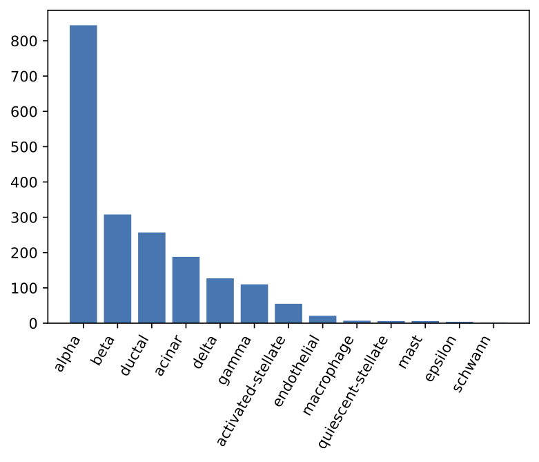
To demonstrate the result of Theorem 1, we design the following experiment. After performing the same pre-processing and balancing steps from the previous experiment, we proceed to remove cells of one fixed type from the CEL-seq2 dataset and cells of another fixed type from the Smart-seq2 dataset. This way, we can ensure the presence of outliers in both sets. Number of cells-per-type are shown in Fig. 7. We only experiment with types beta, gamma, delta, ductal, and acinar because cells of type alpha constitute almost half of the whole dataset and other types have very few cells for the results to be significant. Then we fix a pair of different cell types, remove each from the corresponding dataset, and estimate the real number of inliers (here meaning the number of cells of a type that appears in both datasets) using the algorithm described in Section 3. The results are reported in Table 1. We observe that in most cases the estimated value is slightly underestimated but is an extremely accurate estimate of the true matching size .
| duct. | aci. | ||||
|---|---|---|---|---|---|
| duct. | |||||
| aci. |
6 CONCLUSION AND DISCUSSION
We have analyzed the problem of matching map recovery between two sets of feature-vectors, when the number of true matches is unknown. We focused on two practically relevant settings of this problem. Assuming a lower bound on is available, we proved—under the weakest possible condition on the signal-to-noise ratio—that the -LSS procedure makes no mistake with high probability. More precisely, -LSS provides an estimated map the support of which is included in the support of the true matching map and the values of these two maps coincide on this subset. More importantly, we proposed a procedure for estimating the unknown matching size and proved that it finds the correct value of and the true matching map with high probability. Once again, this holds under the minimal assumption that the signal-to-noise ratio exceeds the minimax separation rate.
Interestingly, our results demonstrate that the minimax rate of separation does not depend on and, more surprisingly, that the absence of the knowledge of has no impact on the minimax rate. These rates are attained by computationally tractable algorithms solving the minimum cost flow problem. Our results are limited to Gaussian noise and to noise levels that are equal across observations. Furthermore, we only tackled the recovery problem, leaving the problem of estimation to future work.
Acknowledgements
This work was supported by the grant Investissements d’Avenir (ANR-11-IDEX0003/Labex Ecodec/ANR-11-LABX-0047), the ADVANCE Research Grant provided by the Foundation for Armenian Science and Technology, and the Yerevan State University.
References
- Ahuja et al. [1992] Ravindra K. Ahuja, Andrew V. Goldberg, James B. Orlin, and Robert Endre Tarjan. Finding minimum-cost flows by double scaling. Math. Program., 53:243–266, 1992. doi: 10.1007/BF01585705. URL https://doi.org/10.1007/BF01585705.
- Azaïs and de Castro [2020] J. M. Azaïs and Y. de Castro. Multiple testing and variable selection along least angle regression’s path, 2020.
- Bai et al. [2020] Xuyang Bai, Zixin Luo, Lei Zhou, Hongbo Fu, Long Quan, and Chiew-Lan Tai. D3feat: Joint learning of dense detection and description of 3d local features. In Proceedings of the IEEE/CVF Conference on Computer Vision and Pattern Recognition (CVPR), June 2020.
- Blanchard et al. [2018] Gilles Blanchard, Alexandra Carpentier, and Maurilio Gutzeit. Minimax Euclidean separation rates for testing convex hypotheses in . Electron. J. Stat., 12(2):3713–3735, 2018. ISSN 1935-7524/e.
- Burnashev [1979] M. V. Burnashev. On the minimax detection of an inaccurately known signal in a white Gaussian noise background. Theory Probab. Appl., 24:107–119, 1979. ISSN 0040-585X; 1095-7219/e.
- Cai and Ma [2022] T Tony Cai and Rong Ma. Matrix reordering for noisy disordered matrices: Optimality and computationally efficient algorithms. arXiv preprint arXiv:2201.06438, 2022.
- Calonder et al. [2010] Michael Calonder, Vincent Lepetit, Christoph Strecha, and Pascal Fua. Brief: Binary robust independent elementary features. In Kostas Daniilidis, Petros Maragos, and Nikos Paragios, editors, Computer Vision – ECCV 2010, pages 778–792, Berlin, Heidelberg, 2010. Springer Berlin Heidelberg. ISBN 978-3-642-15561-1.
- Chen et al. [2010] Jian Chen, Jie Tian, Noah Lee, Jian Zheng, R. Theodore Smith, and Andrew F. Laine. A partial intensity invariant feature descriptor for multimodal retinal image registration. IEEE Transactions on Biomedical Engineering, 57(7):1707–1718, 2010. doi: 10.1109/TBME.2010.2042169.
- Chen et al. [2022a] Li Chen, Rasmus Kyng, Yang P Liu, Richard Peng, Maximilian Probst Gutenberg, and Sushant Sachdeva. Maximum flow and minimum-cost flow in almost-linear time. arXiv preprint arXiv:2203.00671, 2022a.
- Chen et al. [2022b] Shuxiao Chen, Sizun Jiang, Zongming Ma, Garry P Nolan, and Bokai Zhu. One-way matching of datasets with low rank signals. arXiv preprint arXiv:2204.13858, 2022b.
- Chertkov et al. [2010] M. Chertkov, L. Kroc, F. Krzakala, M. Vergassola, L. Zdeborová, and Boris I. Shraiman. Inference in particle tracking experiments by passing messages between images. Proceedings of the National Academy of Sciences of the United States of America, 107(17):7663–7668, 2010. ISSN 00278424. URL http://www.jstor.org/stable/25665416.
- Collier [2012] Olivier Collier. Minimax hypothesis testing for curve registration. In Neil D. Lawrence and Mark A. Girolami, editors, Proceedings of the Fifteenth International Conference on Artificial Intelligence and Statistics, AISTATS 2012, La Palma, Canary Islands, Spain, April 21-23, 2012, volume 22 of JMLR Proceedings, pages 236–245. JMLR.org, 2012.
- Collier and Dalalyan [2013] Olivier Collier and Arnak S. Dalalyan. Permutation estimation and minimax rates of identifiability. Journal of Machine Learning Research, W & CP 31 (AI-STATS 2013):10–19, 2013.
- Collier and Dalalyan [2016] Olivier Collier and Arnak S Dalalyan. Minimax rates in permutation estimation for feature matching. The Journal of Machine Learning Research, 17(1):162–192, 2016.
- Comminges and Dalalyan [2012] Laëtitia Comminges and Arnak S. Dalalyan. Tight conditions for consistency of variable selection in the context of high dimensionality. Ann. Stat., 40(5):2667–2696, 2012. ISSN 0090-5364; 2168-8966/e.
- Comminges and Dalalyan [2013] Laëtitia Comminges and Arnak S. Dalalyan. Minimax testing of a composite null hypothesis defined via a quadratic functional in the model of regression. Electron. J. Stat., 7:146–190, 2013. ISSN 1935-7524/e.
- Flammarion et al. [2019] Nicolas Flammarion, Cheng Mao, and Philippe Rigollet. Optimal rates of statistical seriation. Bernoulli, 25(1):623–653, 2019.
- Fulkerson [1961] Delbert R Fulkerson. An out-of-kilter method for minimal-cost flow problems. Journal of the Society for Industrial and Applied Mathematics, 9(1):18–27, 1961.
- Galil and Tardos [1988] Zvi Galil and Éva Tardos. An min-cost flow algorithm. J. ACM, 35(2):374â386, 1988. ISSN 0004-5411.
- Galstyan et al. [2022] Tigran Galstyan, Arshak Minasyan, and Arnak S. Dalalyan. Optimal detection of the feature matching map in presence of noise and outliers. Electronic Journal of Statistics, 16(2):5720 – 5750, 2022. doi: 10.1214/22-EJS2076. URL https://doi.org/10.1214/22-EJS2076.
- Gao and Zhang [2019] Chao Gao and Anderson Y Zhang. Iterative algorithm for discrete structure recovery. arXiv preprint arXiv:1911.01018, 2019.
- Giraud et al. [2021] Christophe Giraud, Yann Issartel, and Nicolas Verzelen. Localization in 1d non-parametric latent space models from pairwise affinities. arXiv preprint arXiv:2108.03098, 2021.
- Goldberg and Tarjan [1989] Andrew V. Goldberg and Robert E. Tarjan. Finding minimum-cost circulations by canceling negative cycles. J. ACM, 36(4):873â886, 1989.
- Goldberg et al. [2015] A.V. Goldberg, H. Kaplan, S. Hed, and Robert Tarjan. Minimum cost flows in graphs with unit capacities. Leibniz International Proceedings in Informatics, LIPIcs, 30:406–419, 02 2015. doi: 10.4230/LIPIcs.STACS.2015.406.
- Hao et al. [2021] Yuhan Hao, Stephanie Hao, Erica Andersen-Nissen, William M. Mauck III, Shiwei Zheng, Andrew Butler, Maddie J. Lee, Aaron J. Wilk, Charlotte Darby, Michael Zagar, Paul Hoffman, Marlon Stoeckius, Efthymia Papalexi, Eleni P. Mimitou, Jaison Jain, Avi Srivastava, Tim Stuart, Lamar B. Fleming, Bertrand Yeung, Angela J. Rogers, Juliana M. McElrath, Catherine A. Blish, Raphael Gottardo, Peter Smibert, and Rahul Satija. Integrated analysis of multimodal single-cell data. Cell, 2021. doi: 10.1016/j.cell.2021.04.048. URL https://doi.org/10.1016/j.cell.2021.04.048.
- Harwood and Drummond [2016] Ben Harwood and Tom Drummond. Fanng: Fast approximate nearest neighbour graphs. In 2016 IEEE Conference on Computer Vision and Pattern Recognition (CVPR), pages 5713–5722, 2016. doi: 10.1109/CVPR.2016.616.
- Hashimshony et al. [2016] Tamar Hashimshony, Naftalie Senderovich, Gal Avital, Agnes Klochendler, Yaron De Leeuw, Leon Anavy, Dave Gennert, Shuqiang Li, Kenneth J Livak, Orit Rozenblatt-Rosen, et al. Cel-seq2: sensitive highly-multiplexed single-cell rna-seq. Genome biology, 17(1):1–7, 2016.
- Ingster [1982] Yu. I. Ingster. Minimax nonparametric detection of signals in white Gaussian noise. Probl. Inf. Transm., 18:130–140, 1982.
- Ingster and Suslina [2003] Yu. I. Ingster and I. A. Suslina. Nonparametric goodness-of-fit testing under Gaussian models, volume 169 of Lecture Notes in Statistics. Springer-Verlag, New York, 2003.
- Jiang et al. [2016] Zhansheng Jiang, Lingxi Xie, Xiaotie Deng, Weiwei Xu, and Jingdong Wang. Fast nearest neighbor search in the hamming space. In Qi Tian, Nicu Sebe, Guo-Jun Qi, Benoit Huet, Richang Hong, and Xueliang Liu, editors, MultiMedia Modeling, pages 325–336, Cham, 2016. Springer International Publishing. ISBN 978-3-319-27671-7.
- Jin et al. [2020] Yuhe Jin, Dmytro Mishkin, Anastasiia Mishchuk, Jiri Matas, Pascal Fua, Kwang Moo Yi, and Eduard Trulls. Image Matching across Wide Baselines: From Paper to Practice. International Journal of Computer Vision, 2020.
- Juditsky and Nemirovski [2020] Anatoli Juditsky and Arkadin Nemirovski. Statistical inference via convex optimization. Princeton, NJ: Princeton University Press, 2020. ISBN 978-0-691-19729-6/hbk; 978-0-691-20031-6/ebook.
- Kuhn [2012] Harold W. Kuhn. A tale of three eras: The discovery and rediscovery of the hungarian method. Eur. J. Oper. Res., 219(3):641–651, 2012.
- Kunisky and Niles-Weed [2022] Dmitriy Kunisky and Jonathan Niles-Weed. Strong recovery of geometric planted matchings. In Proceedings of the 2022 Annual ACM-SIAM Symposium on Discrete Algorithms (SODA), pages 834–876. SIAM, 2022.
- Lowe [2004] David G Lowe. Distinctive image features from scale-invariant keypoints. International journal of computer vision, 60(2):91–110, 2004.
- Ma et al. [2020] Rong Ma, T Tony Cai, and Hongzhe Li. Optimal permutation recovery in permuted monotone matrix model. Journal of the American Statistical Association, pages 1–15, 2020.
- Malkov and Yashunin [2020] Yu A. Malkov and D. A. Yashunin. Efficient and robust approximate nearest neighbor search using hierarchical navigable small world graphs. IEEE Transactions on Pattern Analysis and Machine Intelligence, 42(4):824–836, 2020. doi: 10.1109/TPAMI.2018.2889473.
- Mao et al. [2018] Cheng Mao, Jonathan Weed, and Philippe Rigollet. Minimax rates and efficient algorithms for noisy sorting. In Algorithmic Learning Theory, pages 821–847. PMLR, 2018.
- Mao et al. [2020] Cheng Mao, Ashwin Pananjady, and Martin J Wainwright. Towards optimal estimation of bivariate isotonic matrices with unknown permutations. Annals of Statistics, 48(6):3183–3205, 2020.
- Ndaoud and Tsybakov [2020] Mohamed Ndaoud and Alexandre B. Tsybakov. Optimal variable selection and adaptive noisy compressed sensing. IEEE Trans. Inf. Theory, 66(4):2517–2532, 2020. ISSN 0018-9448.
- Orlin [1993] James B. Orlin. A faster strongly polynomial minimum cost flow algorithm. Oper. Res., 41(2):338–350, 1993.
- Orlin [1996] James B. Orlin. A polynomial time primal network simplex algorithm for minimum cost flows. In Proceedings of the Seventh Annual ACM-SIAM Symposium on Discrete Algorithms, SODA ’96, page 474â481, USA, 1996. Society for Industrial and Applied Mathematics. ISBN 0898713668.
- Orlin et al. [1993] James B. Orlin, Serge A. Plotkin, and Éva Tardos. Polynomial dual network simplex algorithms. Math. Program., 60(1â3):255â276, 1993.
- Pananjady and Samworth [2020] Ashwin Pananjady and Richard J Samworth. Isotonic regression with unknown permutations: Statistics, computation, and adaptation. arXiv preprint arXiv:2009.02609, 2020.
- Pananjady et al. [2017] Ashwin Pananjady, Martin J Wainwright, and Thomas A Courtade. Linear regression with shuffled data: Statistical and computational limits of permutation recovery. IEEE Transactions on Information Theory, 64(5):3286–3300, 2017.
- Perron and Furnon [2022] Laurent Perron and Vincent Furnon. Or-tools, 2022. URL https://developers.google.com/optimization/.
- Picelli et al. [2013] Simone Picelli, Åsa K Björklund, Omid R Faridani, Sven Sagasser, Gösta Winberg, and Rickard Sandberg. Smart-seq2 for sensitive full-length transcriptome profiling in single cells. Nature methods, 10(11):1096–1098, 2013.
- Ramdas et al. [2016] Aaditya Ramdas, David Isenberg, Aarti Singh, and Larry A. Wasserman. Minimax lower bounds for linear independence testing. In IEEE International Symposium on Information Theory, ISIT 2016, Barcelona, Spain, July 10-15, 2016, pages 965–969. IEEE, 2016.
- Rublee et al. [2011] Ethan Rublee, Vincent Rabaud, Kurt Konolige, and Gary Bradski. Orb: An efficient alternative to sift or surf. In 2011 International Conference on Computer Vision, pages 2564–2571, 2011. doi: 10.1109/ICCV.2011.6126544.
- Shah et al. [2021] Nihar B. Shah, Sivaraman Balakrishnan, and Martin J. Wainwright. A permutation-based model for crowd labeling: Optimal estimation and robustness. IEEE Transactions on Information Theory, 67(6):4162–4184, 2021. doi: 10.1109/TIT.2020.3045613.
- Slawski and Ben-David [2019] Martin Slawski and Emanuel Ben-David. Linear regression with sparsely permuted data. Electronic Journal of Statistics, 13(1):1–36, 2019.
- Tian et al. [2020] Yurun Tian, Vassileios Balntas, Tony Ng, Axel Barroso-Laguna, Yiannis Demiris, and Krystian Mikolajczyk. D2d: Keypoint extraction with describe to detect approach. In Proceedings of the Asian Conference on Computer Vision (ACCV), November 2020.
- Wang et al. [2022] Haoyu Wang, Yihong Wu, Jiaming Xu, and Israel Yoloh. Random graph matching in geometric models: the case of complete graphs. arXiv preprint arXiv:2202.10662, 2022.
- Wang et al. [2018] Ke Wang, Ningyu Zhu, Yao Cheng, Ruifeng Li, Tianxiang Zhou, and Xuexiong Long. Fast feature matching based on r -nearest k -means searching. CAAI Transactions on Intelligence Technology, 3(4):198–207, 2018. doi: https://doi.org/10.1049/trit.2018.1041. URL https://ietresearch.onlinelibrary.wiley.com/doi/abs/10.1049/trit.2018.1041.
- Wei et al. [2019] Yuting Wei, Martin J. Wainwright, and Adityanand Guntuboyina. The geometry of hypothesis testing over convex cones: Generalized likelihood ratio tests and minimax radii. The Annals of Statistics, 47(2):994 – 1024, 2019.
- Wolf et al. [2018] F Alexander Wolf, Philipp Angerer, and Fabian J Theis. Scanpy: large-scale single-cell gene expression data analysis. Genome biology, 19(1):1–5, 2018.
- Wolfer and Kontorovich [2020] Geoffrey Wolfer and Aryeh Kontorovich. Minimax testing of identity to a reference ergodic markov chain. In Silvia Chiappa and Roberto Calandra, editors, The 23rd International Conference on Artificial Intelligence and Statistics, AISTATS 2020, 26-28 August 2020, Online [Palermo, Sicily, Italy], volume 108 of Proceedings of Machine Learning Research, pages 191–201. PMLR, 2020.
- Xing et al. [2020] Xin Xing, Meimei Liu, Ping Ma, and Wenxuan Zhong. Minimax nonparametric parallelism test. Journal of Machine Learning Research, 21(94):1–47, 2020. URL http://jmlr.org/papers/v21/19-800.html.
Appendix
The purpose of this appendix is twofold: to present the proofs of the lemmas used in the main paper and to provide additional experimental evidence showing that it is indeed possible to obtain an accurate estimator for unknown even when the noise levels are unknown and potentially heterogeneous. The reproducible code of all the experiments can be found in the supplementary material.
Appendix A Proofs of Lemmas from Section 4
We start by presenting the definitions that we use in this supplementary material. Recall the definitions of the test statistics and its normalized version , which depends on the quantity
| (37) |
For completeness, we also recall the definition of the standard Gaussian random vectors
| (38) |
The quantities associated with which will be used in the proofs are and , which are defined as follows
| (39) |
Recall also that for any matching map we define as follows
| (40) |
In this section, we present the proofs of lemmas used in Section 3 for proving Theorem 2 and Theorem 3. For the reader’s convenience, we include the statements of the lemmas as well.
See 1
Proof of Lemma 1.
Let us recall the definition of the individual signal-to-noise ratios . For any matching map and for any , we have
| (41) | ||||
| (42) | ||||
| (43) |
Note that if is such that (correct matching), then . For all the other , we have . Therefore, denoting and , Eq. (43) implies that on the event , we have
| (44) | ||||
| (45) |
Let us choose any such that and . We define as the restriction of on . If, in addition, we set , we can infer from the last display that
| (46) | ||||
| (47) | ||||
| (48) | ||||
| (49) |
On the event , we have . Moreover, since , we have . These two inequalities combined with (49) complete the proof of the lemma. ∎
See 2
Proof of Lemma 2.
The union bound implies that
| (50) | ||||
| (51) |
Notice that can be represented as the maximum of absolute values of standard Gaussian random variables, i.e., . Applying the well-known Gaussian tail bounds together with the union bound yields
| (52) |
To bound the second term of (51), we use Lemma 1 from Galstyan et al. [2022] which bounds the tails of a random variable . Thus, combining it with a union bound we arrive at the following inequality
| (53) | ||||
| (54) |
Then, plugging the bounds obtained in (52) and (54) into (51) concludes the proof of the lemma. ∎
See 3
Proof of Lemma 3.
See 4
Proof of Lemma 4.
Let be a matching map from minimizing , i.e., such that . According to Lemma 1, we have for every . One easily checks that there exists a set of cardinality such that and where is the restriction of to . Indeed, if is any element of minimizing , we know that it is defined as a restriction of on some set of cardinality . If we replace arbitrary elements of by those of , and modify accordingly, then we will get a new mapping from , for which the value of is less than or equal to . Therefore, we have found a mapping map that minimizes over and has a support that is obtained by adding one point to . This implies that
| (57) | ||||
| (58) |
This completes the proof of the lemma. ∎
Appendix B Additional experiments on real data
In this section, we perform experiments on a pair of images and respectively choose keypoints on each of them to showcase the behavior of the proposed procedure. In Fig. 5 of the main manuscript, we show the histogram of the choice of matching size for distinct image pairs from “Reichstag” scene of IMC-PT 2020 dataset [Jin et al., 2020]. In this dataset, we only have the pseudo ground truths, and sometimes these ground truths are incorrect (different points are matched), which makes the results unreliable. Therefore, to have a more controlled experiment we take one image of Sacré Coeur of Paris and crop it in half on each axis. Then, we add noise into the cropped image by interpolating the pixels such that both images have the same resolution. This procedure is in line with the studied model, presented in (1). Afterward, we detect and compute SIFT descriptors of keypoints from the cropped image and translate them into the original image. Then, we fix inlier keypoints in both images and add distinct points to each image, which will be considered as outliers.

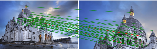
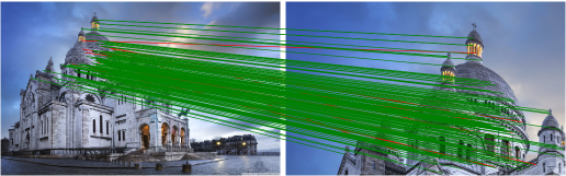
We then run our procedure for the estimation of the matching size and the recovery of the matching map with the tuning parameters chosen as shown in Theorem 1. The results for different values of and are summarized in the figure below. The estimated value is close to and is slightly underestimated in all cases. Slight underestimation is not a problem, whereas slight overestimation would surely cause more incorrect matching pairs.
For all the plots, we see that the value of is estimated accurately and is slightly underestimated (as shown also in Fig. 5). The accuracy of the estimation of (number of green lines) is also very high with only a few mistakes. It is worth mentioning that the estimation of is a procedure that can be of interest by itself because after having an accurate estimator for one is free to apply any matching algorithm to circumvent other purposes. For example, one can use fast approximate methods to accelerate matching algorithms (see e.g. Malkov and Yashunin [2020], Harwood and Drummond [2016], Jiang et al. [2016]). Another possible direction is to consider wider or narrower classes of mappings, e.g. 1-to-many matching maps.