Decimated Prony’s method for stable super-resolution

Abstract

We study recovery of amplitudes and nodes of a finite impulse train from noisy frequency samples. This problem is known as super-resolution under sparsity constraints and has numerous applications. An especially challenging scenario occurs when the separation between Dirac pulses is smaller than the Nyquist-Shannon-Rayleigh limit. Despite large volumes of research and well-established worst-case recovery bounds, there is currently no known computationally efficient method which achieves these bounds in practice. In this work we combine the well-known Prony’s method for exponential fitting with a recently established decimation technique for analyzing the super-resolution problem in the above mentioned regime. We show that our approach attains optimal asymptotic stability in the presence of noise, and has lower computational complexity than the current state of the art methods.

I Introduction

Various problems of signal reconstruction in multiple basic and applied settings can be reduced to recovering the amplitudes $\left\{\alpha_{k}\right\}_{k=1}^{n}$ and nodes $\left\{x_{k}\right\}_{k=1}^{n}$ of a finite impulse train $f(x)=\sum_{k=1}^{n}\alpha_{k}\delta(x-x_{k})$ from band-limited and noisy spectral measurements

$$g(\omega)=\sum_{k=1}^{n}\alpha_{k}e^{2\pi\mathrm{j}x_{k}\omega}+e(\omega),\quad\omega\in[-\Omega,\Omega],$$ (1)

where $\Omega>0$ and $\left\|e\right\|_{\infty}\leq\epsilon$ for some $\epsilon>0$. Due to its widespread applications, this problem has been studied under various guises including tauberian approximation [1], parametric spectrum estimation and direction of arrival [2, 3], time-delay estimation [4], sparse deconvolution [5], super-resolution (SR) [6, 7] and finite-rate-of-innovation sampling [8, 9]. Beyond the theoretical modelling, recent advances have shown (1) to be the work-horse for emerging areas such as super-resolution tomography and spectroscopy [10, 11], ultra-fast time-of-flight imaging [12] and unlimited sensing [13]; in such cases, efficient and robust solutions to (1) entail pushing real-world capabilities beyond the possibilities of conventional hardware.

Despite the theoretical advances on this topic (works cited above and follow-up literature), there are still fundamental research gaps that arise due to ill-posedness and instability of (1) in the presence of noise. In particular, an especially challenging regime occurs when the separation $\Delta$ between two or more nodes is smaller than the Nyquist-Shannon-Rayleigh (NSR) limit $1/\Omega$. Recently, min-max error bounds for SR in the noisy regime were derived in the case when some nodes form a dense cluster [14, 15, 16], establishing the fundamental limits of recovery in the SR problem (cf. Sect. II). However, a tractable and provably optimal algorithm has been missing from the literature.

In this work we develop a reconstruction algorithm inspired by the decimation approach [17, 18] (cf.[19, 14, 16, 15] and also [20, 21]). Our procedure (Sect. III) relies on sampling $g(\omega)$ at $2n$ equispaced and maximally separated frequencies, followed by solving the SR problem thus obtained by applying the classical Prony’s method for exponential fitting [22], whose accuracy has been recently established in [23]. For success of the approach, care needs to be taken to avoid node aliasing and collisions. Inspired by [15], this is achieved by considering sufficiently many decimated sub-problems. The result is a tractable algorithm, dubbed the Decimated Prony’s method (DPM), which has lower computational complexity than the well-established and frequently used ESPRIT algorithm (see e.g. [24]). We further provide theoretical and numerical evidence which show that DPM achieves the optimal asymptotic stability and noise tolerance guaranteed in the literature. We believe that our results pave the way to developing robust procedures for optimal solution of problems derived from (1).

II Towards optimal algorithms

Throughout the paper we consider the number of nodes (resp. amplitudes) $n\in\left\{1,2,\dots\right\}$ in (1) to be fixed. We assume that the nodes satisfy $\left\{x_{k}\right\}_{k=1}^{n}\subseteq\left[-\frac{1}{2},\frac{1}{2}\right]$. By rescaling the data (1), this assumption poses no loss of generality (see Section 4 in [15]). Let $\left\{\tilde{x}_{k}\right\}_{k=1}^{n}$ and $\left\{\tilde{\alpha}_{k}\right\}_{k=1}^{n}$ be the approximated parameters obtained via a reconstruction algorithm using the data (1).

Definition 1 ([15]).

Let $\left\{(\alpha_{k},x_{k})\right\}_{k=1}^{n}\subseteq U$. Given $\epsilon>0$, the min-max recovery rates are

$$\Lambda^{x,j}_{\epsilon,U,\Omega}=\inf_{\mathcal{A}:g\mapsto\left\{\tilde{\alpha}_{j},\tilde{x}_{j}\right\}}\ \sup_{\left\{\alpha_{j},x_{j}\right\}}\ \sup_{\|e\|_{\infty}\leq\epsilon}\left|x_{j}-\tilde{x_{j}}\right|,$$

$$\Lambda^{\alpha,j}_{\epsilon,U,\Omega}=\inf_{\mathcal{A}:g\mapsto\left\{\tilde{\alpha}_{j},\tilde{x}_{j}\right\}}\ \sup_{\left\{\alpha_{j},x_{j}\right\}}\sup_{\|e\|_{\infty}\leq\epsilon}\left|\alpha_{j}-\tilde{\alpha}_{j}\right|.$$

Here $U$ is some fixed subset in the parameter space, whereas the infimum is over the set of all reconstruction algorithms $\mathcal{A}$ which employ the data (1).

The min-max rates define the optimal recovery rates achievable by a reconstruction algorithm, in the presence of measurement noise of magnitude less than $\epsilon$ and when the node and amplitude pairs belong to $U$.

It has been well established that the difficulty of SR is related to the minimal separation between nodes, $\Delta:=\min_{s\neq k}|x_{s}-x_{k}|$. A particular case of interest, both theoretically and from an applications perspective, concerns signals whose nodes are densely clustered, i.e. $\Delta\ll\frac{1}{\Omega}$ [25, 26, 27, 28, 29, 30].

Definition 2.

We call $\{x_{k}\}_{k=1}^{n}$ a clustered configuration if there is a partition of the nodes into clusters such that the distances between the nodes in each cluster are on the order of $\Delta$, while the inter-cluster distances are on the order of $1/\Omega$ (well-separated clusters). [14, 15].

Theorem 1 ([15]).

Let the super-resolution factor satisfy $\textrm{SRF}:={1\over{\Omega\Delta}}\gtrapprox 1$, and $\{|\alpha_{k}|\}_{k=1}^{n}$ be (uniformly) bounded. Let there exist a single cluster $\mathcal{X}$ of size $1<\ell<n$, whereas all other (singleton) clusters are well-separated, and $\epsilon\lessapprox(\Omega\Delta)^{2\ell-1}$. Then

$$\Lambda^{x,j}_{\epsilon,U,\Omega}\asymp\begin{cases}\textrm{SRF}^{2\ell-2}\frac{\epsilon}{\Omega}&x_{j}\in\mathcal{X},\\ {\epsilon\over\Omega}&x_{j}\notin\mathcal{X},\end{cases}$$

$$\Lambda^{\alpha,j}_{\epsilon,U,\Omega}\asymp\begin{cases}\textrm{SRF}^{2\ell-1}\epsilon&x_{j}\in\mathcal{X},\\ \epsilon&x_{j}\notin\mathcal{X}.\end{cases}$$

Here, $\lessapprox,\gtrapprox,\asymp$ denote asymptotic inequalities/equivalence up to multiplying constants independent of $\Omega,\Delta$, $\epsilon$, while $U$ is the set of signals satisfying the assumptions above.

The min-max bounds establish fundamental recovery limits in any application modeled by (1) (e.g. [31]). Related results are known in the signal processing literature for Gaussian noise [27, 29, 32]. Despite a plethora of methods to solve this problem, up to date a tractable algorithm which achieves the min-max rates is missing from the literature. In particular, the frequently used ESPRIT algorithm is sub-optimal, both in terms of the bounds and the threshold SNR [24].

While the proof of Theorem 1 is non-constructive, it motivates a design of an algorithm achieving the optimal rates in practice. Let $\mathcal{J}:=\left[\frac{1}{2}\frac{\Omega}{2n-1},\frac{\Omega}{2n-1}\right]$. For a decimation parameter $\lambda\in\mathcal{J}$, the measurements $\{g(\lambda k)\}_{k=0}^{2n-1}$ yield the problem (1) with $\{e^{2\pi\mathrm{j}x_{j}}\}_{j=1}^{n}$ replaced by $\{e^{2\pi\mathrm{j}\lambda x_{j}}\}_{j=1}^{n}$. By [15, Prop. 5.8] there exists an interval $\mathcal{I}\subset\mathcal{J}$ of length $|\mathcal{I}|\geq c\Omega$ such that every $\lambda\in\mathcal{I}$ satisfies $|e^{2\pi\mathrm{j}\lambda x_{i}}-e^{2\pi\mathrm{j}\lambda x_{j}}|\geq n^{-2}$, whenever $x_{i},x_{j}$ belong to different clusters (collision avoidance). By [15, Prop. 5.12], for a collision-avoiding $\lambda$, the condition number of the (theoretical) solution map $\mathcal{P}_{n}$ which inverts (1) in the case $e\equiv 0$ and $\omega\in\left\{k\lambda\right\}_{k=0}^{2n-1}$ matches the min-max rates. Set $\{\tilde{\alpha}_{j},e^{2\pi\mathrm{j}\tilde{y}_{\lambda,j}}\}_{j=1}^{n}=\mathcal{P}_{n}\left\{g(\lambda k)\right\}_{k=0}^{2n-1}$. Let the set of all aliased solutions corresponding to $\{\tilde{y}_{\lambda,j}\}_{j=1}^{n}$ be

$$X_{\lambda}:=\bigcup_{j=1}^{n}\bigg{\{}\left(\lambda,t\right):\ t=\frac{\tilde{y}_{\lambda,j}+m}{\lambda},m\in\mathbb{Z},\left|t\right|\leq\frac{1}{2}\bigg{\}},$$ (2)

where the aliasing follows by periodicity of $y\mapsto e^{2\pi\mathrm{j}y}$. The arguments above imply that $X_{\lambda}$ contains at least one element $(\lambda,t)$ with $t\approx x_{j}$ for each $j=1,\dots,n$ (call it Property P*). Thus, to obtain a constructive procedure for recovery, we propose the following general approach:

1. Find a collision-avoiding $\lambda\in\mathcal{J}$;

2. Compute $\{\tilde{\alpha}_{j},e^{2\pi\mathrm{j}\tilde{y}_{\lambda,j}}\}_{j=1}^{n}\approx\mathcal{P}_{n}\left\{g(\lambda k)\right\}_{k=0}^{2n-1}$ with optimal stability/accuracy;

3. Find $\{(\lambda,\tilde{x}_{j})\}_{j=1}^{n}\subset X_{\lambda}$ s.t. $\tilde{x}_{j}\approx x_{j}$ (dealiasing).

In this work we tackle steps 1 and 3. For step 2, we propose to use the classical Prony’s method [22] (see Alg. II.1), which provides an exact solution to the problem in the noiseless regime. The use of Prony’s method is justified by our recent results in [23] which prove its optimality in the regime $\Delta\ll 1$ and $\Omega$ fixed (corresponding to $\textrm{SRF}\gg 1$ in Thm. 1).

Theorem 2 ([23]).

Suppose $\ell_{*}$ is the largest cluster size, and each $x_{j}$ belongs to a cluster of size $\ell_{j}$. For $\epsilon\lessapprox\Delta^{2\ell_{*}-1}$, the output of Alg. II.1 satisfies: $|x_{j}-\tilde{x}_{j}|\lessapprox\Delta^{2-2\ell_{j}}\epsilon$ for the nodes, and $|\alpha_{j}-\tilde{\alpha}_{j}|\lessapprox\Delta^{t_{j}}\epsilon$ for the amplitudes, where $t_{j}=1-2\ell_{j}$ if $\ell_{j}>1$, with $t_{j}=0$ if $\ell_{j}=1$.

Define the node/amplitude error amplification factors

$$\mathcal{K}_{x,j}:=\epsilon^{-1}\Omega|x_{j}-\tilde{x}_{j}|,\quad\mathcal{K}_{\alpha,j}:=\epsilon^{-1}|\alpha_{j}-\tilde{\alpha}_{j}|.$$

Fixing $\Omega=2n-1$ for $n\in\left\{3,4,5\right\}$ and cluster sizes $\ell\in\{2,3,5\}$, Fig. 1 shows that, indeed, both $\mathcal{K}_{x,j}$ and $\mathcal{K}_{\alpha,j}$ computed by Alg. II.1 scale as the min-max rates above.

Remark 1.

In all numerical tests in this paper, we follow [15] and consider $x_{k}$ to be successfully recovered if the error $|x_{k}-\tilde{x}_{k}|$ is smaller than one third of the distance between $x_{k}$ and its nearest neighbor.

1

Input : Sequence $\{\tilde{m}_{k}\equiv g(k)\}_{k=0}^{2n-1}$

Output : Estimates $\{\tilde{x}_{k},\ \tilde{\alpha}_{k}\}_{k=1}^{n}$

Notation : $\operatorname{col}\left\{y_{k}\right\}_{k=1}^{m}=[y_{1},\dots,y_{m}]^{\top}\in\mathbb{C}^{m}$.

2 Construct $\tilde{H}_{n}=\left(\tilde{m}_{i+j}\right)_{0\leq i,j\leq n-1}$

3 Solve the linear least squares problem

$$\operatorname{col}\left\{q_{k}\right\}_{k=0}^{n-1}=\underset{\boldsymbol{q}\in\mathbb{C}^{n}}{\operatorname*{arg\,min}}\big{\|}\tilde{H}_{n}\boldsymbol{q}+\operatorname{col}\left\{\tilde{m}_{k}\right\}_{k=n}^{2n-1}\big{\|}_{2}$$

4 Compute $\{\tilde{z}_{k}\}_{k=1}^{n}$ as the roots of the (perturbed) Prony polynomial $q(z):=z^{n}+\sum_{j=0}^{n-1}q_{j}z^{j}$.

5 Recover $\left\{\tilde{x}_{k}\right\}_{k=1}^{n}$ from $\tilde{z}_{k}$ via $\tilde{x}_{k}=\frac{\operatorname{Arg}(\tilde{z}_{k})}{2\pi}$.

Construct $\tilde{V}=\left(\tilde{z}_{k}^{i}\right)_{i=0,\dots,n-1}^{k=1,\dots,n}$ and solve $\operatorname{col}\left\{\tilde{\alpha}_{k}\right\}_{k=1}^{n}=\underset{\boldsymbol{\alpha}\in\mathbb{C}^{n}}{\operatorname*{arg\,min}}\big{\|}\tilde{V}\boldsymbol{\alpha}-\operatorname{col}\left\{\tilde{m}_{k}\right\}_{k=0}^{n-1}\big{\|}_{2}$ return the estimated parameters $\left\{\tilde{x}_{k},\tilde{\alpha}_{k}\right\}_{k=1}^{n}$

Algorithm II.1 The Classical Prony method

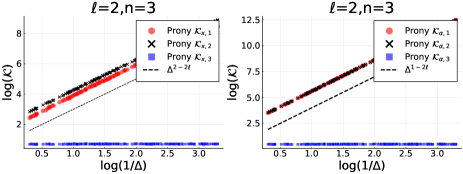
(a) Error amplification factors for $\ell=2,n=3$

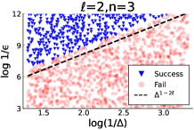
(b) Recovery SNR threshold

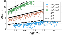
(c) $\mathcal{K}_{x,1}$ for various $\ell,n$

Figure 1: Classical Prony method - asymptotic optimality. (a) For cluster nodes, $\left\{\mathcal{K}_{x,j}\right\}$ (left) scale like $\Delta^{2-2\ell}$, while $\left\{\mathcal{K}_{\alpha,j}\right\}$ (right) scale like $\Delta^{1-2\ell}$. For the non-cluster node $j=3$, $\left\{\mathcal{K}_{x,j}\right\}$ and $\left\{\mathcal{K}_{\alpha,j}\right\}$ are lower bounded by a constant. (b) Noise threshold for recovery of cluster nodes scales like $\Delta^{2\ell-1}$. (c) $\mathcal{K}_{x,j}\asymp\Delta^{2-2\ell}$ for cluster nodes holds for different $\ell,n$. The number of tests is (a) 200, (b) 2000, (c) 200 for each $\ell,n$.

III Decimated Prony’s method

Here we develop the Decimated Prony’s Method (DPM) (Alg. III.1). To find a collision-avoiding $\lambda$, we consider $X_{\lambda}$ as in (2) for each $\lambda\in G$ where $G=\operatorname{linspace}(\mathcal{J},N_{\lambda})$ is the uniform grid of size $N_{\lambda}\in\mathbb{N}$ (the choice of $N_{\lambda}$ is motivated in Remark 2. Cf. Fig. 2 for a numerical justification of this approach) [steps 1–5]. Next, we compute the histogram of $\{x:(\lambda,x)\in\bigcup_{\lambda\in G}X_{\lambda}\}$ with $N_{b}$ bins and find the $n$ bins $\{B_{j}\}_{j=1}^{n}$ with largest counts [step 6]. Following the criterion for successful node recovery (see Remark 1), $N_{b}$ is set to $3\Delta^{-1}$. Based on [15] we expect the set

$$\Lambda:=\bigcap_{k=1}^{n}\{\lambda:(\lambda,x)\in\bigcup_{\lambda\in G}X_{\lambda}\wedge x\in B_{k}\}$$ (3)

to contain only collision-avoiding $\lambda$’s. In particular, if $\lambda$ is not collision-avoiding, Property P* will not be satisfied since at least two nodes will be ill-conditioned. Furthermore, the proof of [15, Prop. 5.17] suggests that if $\lambda_{1}\neq\lambda_{2}$ are collision-avoiding, then, with high probability, $(\lambda_{1},t_{1})\in X_{\lambda_{1}}$ and $(\lambda_{2},t_{2})\in X_{\lambda_{2}}$ with $t_{1}\approx t_{2}$ implies $t_{1}\approx t_{2}\approx x_{j}$ for some $j=1,\dots,n$. Thus, provided $\Lambda\neq\emptyset$ (otherwise the algorithm fails), we choose $\lambda^{*}=\max\Lambda$ to obtain maximal in-cluster separaton of $\{e^{2\pi\mathrm{j}\lambda^{*}x_{j}}\}_{j=1}^{n}$ [step 7] and recover the corresponding $\{\tilde{x}_{j}\}_{j=1}^{n}$ by choosing $\tilde{x}_{j}\in B_{j}$ s.t. $(\lambda^{*},\tilde{x}_{j})\in X_{\lambda^{*}}$ [step 8]. Finally, the amplitude approximations are found by solving a Vandermonde system [step 9].

We are able to prove (see the Appendix) correctness of DPM in a special case of single cluster (i.e. $\ell=n$).

Theorem 3.

In the notations of Thm. 1, suppose $\ell=n$. Under a further technical assumption (to be elaborated in the proof), and with the choice of $N_{\lambda}=O(\Omega)$ and $N_{b}=3\Delta^{-1}$, Alg. III.1 attains the bounds of Thm. 1.

Remark 2.

We conjecture that the choices $N_{\lambda}\gtrapprox\Omega$ and $N_{b}\approx\Delta^{-1}$ are sufficient to ensure correctness of the algorithm in the general case. We leave the rigorous justification of this claim to future work. As a guideline, increasing $N_{\lambda}$ is expected to improve the robustness of the DPM.

Next, we analyze the time complexity of DPM by addressing each step of Alg. III.1. Below we use the notation $O=O_{n}$ (recall that $n$ is considered fixed). The classical Prony’s method has complexity $O(1)$, since it depends only on $n$. For every $\lambda\in G$ we apply Alg. II.1 with the samples $\left\{g(\lambda k)\right\}$ and compute $X_{\lambda}$ in (2), which costs $O(N_{\lambda}+\lambda N_{\lambda})$. Computing the histogram with $N_{b}$ bins for data of size $\sum_{i=1}^{N_{\lambda}}n\lambda_{i}$ costs $O(N_{\lambda}\Omega+N_{b})$. Finding the bins $\left\{B_{k}\right\}_{k=1}^{n}$ with $n$ largest counts costs $O(N_{b})$. Computing $\Lambda$ in (3) and $\lambda^{*}=\max\Lambda$, together with finding the estimated $\{\tilde{x}_{k}\}_{k=1}^{n}$ costs $O(N_{\lambda})$. Finally, solving an $n$-order Vandermonde system costs $O(1)$ [33]. Thus, the total complexity is $O(N_{\lambda}\Omega+N_{b})$. As mentioned in Remark 2, $N_{\lambda}\gtrapprox\Omega$ and $N_{b}\gtrapprox\Delta^{-1}$ are expected to be sufficient for correctness of DPM. This gives overall complexity $O(\Omega^{2})+O(\Delta^{-1})$. For small $\Omega$ the dominating factor is $\Delta^{-1}$, in which case we may take $N_{\lambda}=O(\textrm{SRF})$ to have maximal robustness. Otherwise, for large $\Omega$ the dominating factor is $O(\Omega^{2})$. For comparison, the widely used ESPRIT method [2] has a time complexity of order $O(\Omega^{3})$: it includes three SVD decompositions and several matrix multiplications of order $O(\Omega)\times O(\Omega)$.

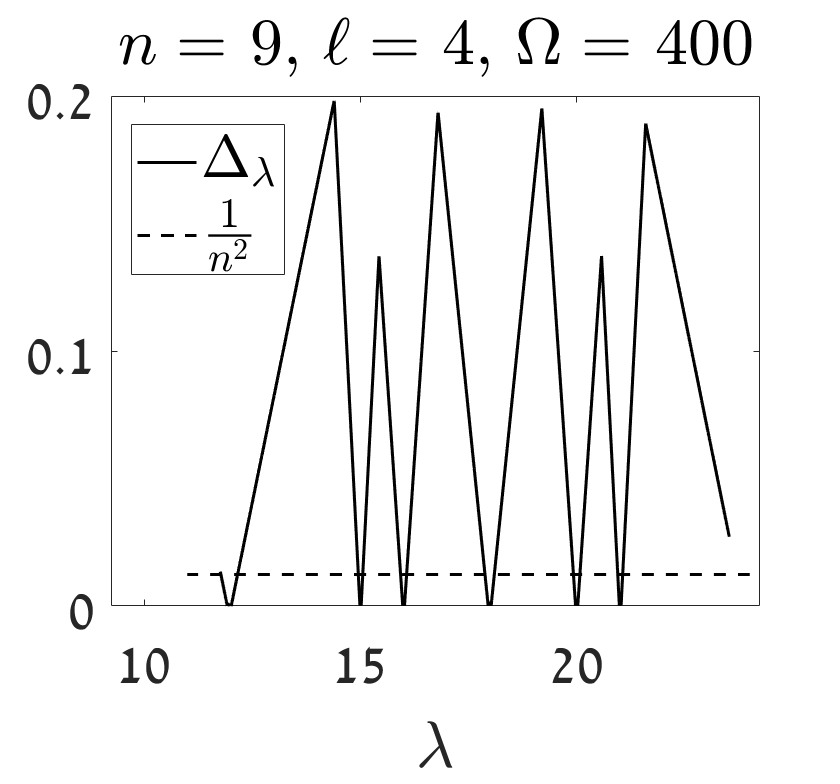
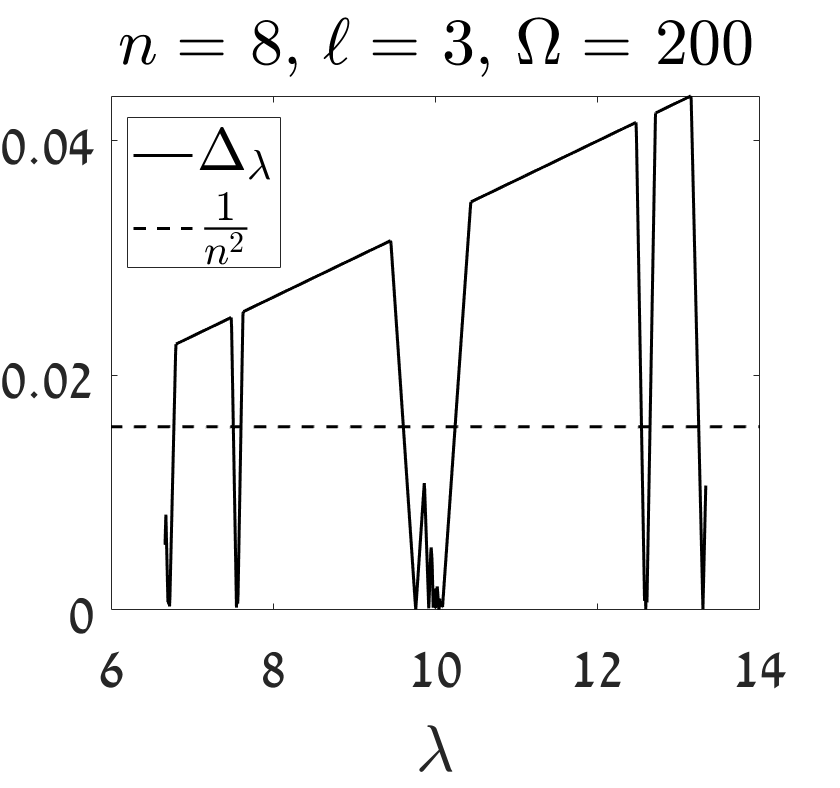
Figure 2: The separation $\Delta_{\lambda}:=\min_{s\neq k}\left|\operatorname{arg}\left(e^{2\pi\mathrm{j}\lambda(x_{k}-x_{s})}\right)\right|$ as a function of $\lambda$, for the single (left) and multi-cluster (right) cases. We see that most $\lambda\in G$ satisfy $\Delta_{\lambda}>\frac{1}{n^{2}}$, i.e. are collision-avoiding. Here we set $N_{\lambda}=\Omega$.

Data : $N_{\lambda},n,\Omega,N_{b}$

Input : $g(\omega)$ as in (1)

Output : Estimates $\{\tilde{x}_{k},\ \tilde{\alpha}_{k}\}_{k=1}^{n}$

1

2for $\lambda\in G:=\operatorname{linspace}(\mathcal{J},N_{\lambda})$ do

3       $\tilde{m}^{(\lambda)}:=\left\{\tilde{m}^{(\lambda)}_{k}=g(\lambda k)\right\}_{k=0}^{2n-1}$

4       $\{e^{2\pi\mathrm{j}\tilde{y}_{\lambda,k}},\tilde{\alpha}_{\lambda,k}\}\longleftarrow\operatorname{Prony}\left(\tilde{m}^{(\lambda)}\right)$

5       Compute $X_{\lambda}$ as in (2)

6

7$X\longleftarrow\bigcup_{\lambda\in G}X_{\lambda}$

8 Compute $H$ - Histogram of $\{x:(\lambda,x)\in X\}$ with $N_{b}$ bins. Set $\left\{B_{k}\right\}_{k=1}^{n}=$ ArgMax($H,n$)

9 Compute $\Lambda$ as in (3) and $\lambda^{*}\xleftarrow{}\max\{\lambda:\lambda\in\Lambda\}$

10 $\{\tilde{x}_{j}\}_{j=1}^{n}\longleftarrow\{x:(\lambda^{*},x)\in X_{\lambda^{*}}\wedge x\in B_{j}\}$

11 Construct $\tilde{V}=\left(e^{2\pi\mathrm{j}\tilde{x}_{j}k\lambda^{*}}\right)_{k=0,\dots,n-1}^{j=1,\dots,n}$ and solve $\operatorname{col}\left\{\tilde{\alpha}_{k}\right\}_{k=1}^{n}=\underset{\boldsymbol{\alpha}\in\mathbb{C}^{n}}{\operatorname*{arg\,min}}\biggl{\|}\tilde{V}\boldsymbol{\alpha}-\operatorname{col}\left\{\tilde{m}_{k}^{(\lambda^{*})}\right\}_{k=0}^{n-1}\biggr{\|}_{2}$

return the estimates $\{\tilde{x}_{k},\ \tilde{\alpha}_{k}\}_{k=1}^{n}$

Algorithm III.1 Decimated Prony Method

We perform reconstruction tests of a signal with random complex amplitudes and measurement noise in a single-cluster configuration with $\ell<n$, where $\epsilon,\Omega,\Delta$ are chosen uniformly at random. The results appear in Fig. 3. We also investigate the noise threshold $\epsilon\lessapprox\textrm{SRF}^{1-2\ell}$ for successful recovery (see Remark 1), and compare to Thm. 1 by recording the success/failure result of each experiment. These results provide numerical validation of the optimality of DPM both in terms of the SNR threshold and the attained estimation accuracy.

Finally, we compare the performance of DPM with the ESPRIT method. Fixing $\ell=2,n=3$, $\Delta=10^{-2.8},\Omega=10^{2.5}$ and running 50 tests for each of 10 values of $\epsilon$ between $10^{-3.5}$ and $10^{-2}$, the mean absolute error in recovering the cluster node is comparable between the two methods. However, DPM with $N_{\lambda}=50$ runs about 7 times faster (Fig. 3(c)).

IV Discussion

Future research avenues include a rigorous proof of the algorithm’s correctness in the general case and improving its robustness, building upon the theory developed in [15, 23]. We believe our method can be extended to higher dimensions, along the lines of recent works such as [34].

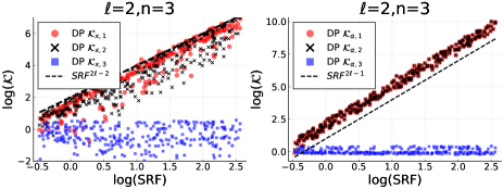
(a) Error amplification factors for $\ell=2,n=3$.

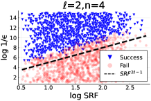
(b) Recovery SNR threshold.

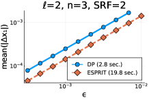
(c) DPM vs. ESPRIT.

Figure 3: DPM - asymptotic optimality. (a) For cluster nodes, $\left\{\mathcal{K}_{x,j}\right\}$ (left) scale like ${\textrm{SRF}}^{2\ell-2}$, while the $\left\{\mathcal{K}_{\alpha,j}\right\}$ (right) scale like ${\textrm{SRF}}^{2\ell-1}$ ($\textrm{SRF}=(\Omega\Delta)^{-1}$). For the non-cluster node $j=3$, both $\left\{\mathcal{K}_{x,j}\right\}$ and $\left\{\mathcal{K}_{\alpha,j}\right\}$ are lower bounded by a constant. Here $N_{\lambda}=10$ and number of tests=$300$. (b) Noise threshold for recovery of cluster nodes scales with ${\textrm{SRF}}^{2\ell-1}$. Here $N_{\lambda}=50$ and number of tests=$2000$. (c) Comparison of accuracy and runtime with the ESPRIT method. While the mean absolute errors (50 tests for each $\epsilon$) scale the same and are comparable, the DPM runs 7 times faster ($N_{\lambda}=50$).

Here we prove Thm. 3. Recall $\mathcal{J}=\left[\frac{1}{2}\frac{\Omega}{2n-1},\frac{\Omega}{2n-1}\right]$. Note that in our case (a single cluster) each $\lambda\in\mathcal{J}$ is collision-avoiding. Hence, we only need to show that the bins $\{B_{j}\}_{j=1}^{n}$ contain $N_{\lambda}$ valid node approximations. We shall use the following technical result.

Proposition 4.

Let $h,\eta>0$ be arbitrary. There exist constants $K_{1}(n),K_{2}(n)$ such that for each $h<|c|\leq\eta/6$ and each $\Omega\in\left[{K_{1}\over\eta},{K_{2}\over h}\right]$ there exists an interval $I\subset\mathcal{J}$ of length $|I|=\eta^{-1}$ satisfying

$$\forall\lambda\in I,\;\forall k\in\mathbb{Z}\qquad\left|c-\frac{k}{\lambda}\right|>h.$$

Proof.

This is just a simplified version of [15, Prop. F.3]. In the proof, the interval $I_{1}$ in case 1 may be replaced by any $I\subset\mathcal{J}$ of length $\eta^{-1}$ and appropriate adjustment of the constants $K_{1},K_{2}$; in case 2 the interval $I$ can be taken as $I_{5}$ itself. ∎

Proof of Thm. 3.

Without loss of generality we assume that $x_{j}\in[-\tilde{h},\tilde{h}]$ for each $j=1,\dots,n$ where $\tilde{h}=\tau\Delta$. Now suppose $\lambda_{0}\in G$ and introduce the auxiliary parameter $a<\min(1/6,\tau)$. Letting $\epsilon\lessapprox\Delta^{2n-1}$ be small enough and employing Thm. 2, the set $X_{\lambda_{0}}$ in (2) can be guaranteed to have form $X_{\lambda_{0}}=\bigcup_{m\in R(\lambda_{0})}X_{\lambda_{0},m}$, where

$$R(\lambda_{0})=\biggl{\{}-\biggl{\lfloor}\frac{\lambda_{0}}{2}\biggr{\rfloor},\dots,\biggl{\lfloor}\frac{\lambda_{0}}{2}\biggr{\rfloor}\biggr{\}}$$

where

$$X_{\lambda_{0},m}=\biggl{\{}\tilde{x}_{j,\lambda_{0}}+\frac{m}{\lambda_{0}}\biggr{\}}_{j=1}^{n},\;|\tilde{x}_{j,\lambda_{0}}-x_{j}|\leq a\Delta.$$

Now recall step 6 in Alg. III.1. We make the following

Genericity assumption: The distance from $x_{j}$ to its closest bin edge is at least $a\Delta$.

For each $\lambda^{\prime}\in G$, $|\tilde{x}_{j,\lambda_{0}}-\tilde{x}_{j,\lambda^{\prime}}|\leq 2a\Delta<\Delta/3$. Therefore, both $\tilde{x}_{j,\lambda_{0}},\tilde{x}_{j,\lambda^{\prime}}$ must belong to the same bin. In particular, we are guaranteed the existence of $n$ bins containing at least $N_{\lambda}$ elements each.

Fix $m\in R(\lambda_{0})\setminus\{0\}$. The choice of $a$ guarantees $X_{\lambda_{0},m}\subset c+\left[-2\tilde{h},2\tilde{h}\right]$ where $c:=\frac{m}{\lambda_{0}}$. Put $h=6\tilde{h}$. Since $|c|\geqslant\lambda_{0}^{-1}\geqslant\frac{2n-1}{\Omega}$, the condition $|c|>h$ holds whenever $\textrm{SRF}>\textrm{const}$. Thus we can apply Prop. 4 with $\eta=3$ and $h,c$ as above, and conclude that there exists $I_{m}\subset\mathcal{J}$ of length $|I_{m}|=1/3$ s.t.

$$\forall\lambda\in I_{m},\;\forall k\in\mathbb{Z}:\qquad\biggl{|}\frac{m}{\lambda_{0}}-\frac{k}{\lambda}\biggr{|}>6\tilde{h}.$$ (4)

By choosing $N_{\lambda}\geq C_{1}\Omega$ for sufficiently large $C_{1}$, we can ensure that there exists $\lambda_{m}\in I_{m}\bigcap G$. Therefore, for each $k\in\mathbb{Z}$, (4) implies that

$$X_{\lambda_{m},k} \subset\left[-1/2,1/2\right]\setminus\biggl{(}\frac{m}{\lambda_{0}}+\left[-2\tilde{h},2\tilde{h}\right]\biggr{)}.$$

Since $X_{\lambda_{0},m}\subset\frac{m}{\lambda_{0}}+\left[-2\tilde{h},2\tilde{h}\right]$, we conclude that $\tilde{x}_{j,\lambda_{0}}+\frac{m}{\lambda_{0}}$ and $\tilde{x}_{j,\lambda_{m}}+\frac{k}{\lambda_{m}}$ cannot belong to the same bin. In particular, the bin containing $\tilde{x}_{j,\lambda_{0}}+\frac{m}{\lambda_{0}}$ contains at most $N_{\lambda}-1$ elements.

Since $\lambda_{0}$ and $m$ were arbitrary, we have shown that the bins containing $\{\tilde{x}_{j,\lambda}:\lambda\in G\}$ have counts at least $N_{\lambda}$ for each $j=1,\dots,n$, while all other bins have strictly smaller counts. Thus, the former bins will be selected when thresholding the histogram. ∎

Remark 3.

The genericity assumption is a technical and not an essential restriction. Alg. III.1 can be easily modified to account for the case that all valid approximations to a node $x_{j}$ belong to two neighboring bins.

References

- [1] Rui J. P. De Figueiredo and Chia-Ling Hu, “Waveform Feature Extraction Based on Tauberian Approximation,” IEEE Transactions on Pattern Analysis and Machine Intelligence, vol. PAMI-4, no. 2, Mar. 1982.
- [2] P. Stoica and R.L. Moses, Spectral Analysis of Signals, Pearson/Prentice Hall, 2005.
- [3] Roland Badeau, Bertrand David, and Gaël Richard, “High-resolution spectral analysis of mixtures of complex exponentials modulated by polynomials,” Signal Processing, IEEE Transactions on, vol. 54, no. 4, 2006.
- [4] I. Kirsteins, “High resolution time delay estimation,” in ICASSP ’87. IEEE International Conference on Acoustics, Speech, and Signal Processing, Apr. 1987, vol. 12.
- [5] Lei Li and Terence P. Speed, “Parametric deconvolution of positive spike trains,” Annals of Statistics, 2000.
- [6] D.L. Donoho, “Superresolution via sparsity constraints,” SIAM Journal on Mathematical Analysis, vol. 23, no. 5, 1992.
- [7] Emmanuel J. Candès and Carlos Fernandez-Granda, “Towards a Mathematical Theory of Super-resolution,” Communications on Pure and Applied Mathematics, vol. 67, no. 6, June 2014.
- [8] M. Vetterli, P. Marziliano, and T. Blu, “Sampling signals with finite rate of innovation,” IEEE Transactions on Signal Processing, vol. 50, no. 6, 2002.
- [9] T. Blu, P.-L. Dragotti, M. Vetterli, P. Marziliano, and L. Coulot, “Sparse Sampling of Signal Innovations,” IEEE Signal Processing Magazine, vol. 25, no. 2, Mar. 2008.
- [10] Chandra Sekhar Seelamantula and Satish Mulleti, “Super-resolution reconstruction in frequency-domain optical-coherence tomography using the finite-rate-of-innovation principle,” IEEE Transactions on Signal Processing, vol. 62, no. 19, 2014.
- [11] Satish Mulleti, Amrinder Singh, Varsha P. Brahmkhatri, Kousik Chandra, Tahseen Raza, Sulakshana P. Mukherjee, Chandra Sekhar Seelamantula, and Hanudatta S. Atreya, “Super-Resolved Nuclear Magnetic Resonance Spectroscopy,” Scientific Reports, vol. 7, no. 1, Aug. 2017.
- [12] A. Bhandari and R. Raskar, “Signal Processing for Time-of-Flight Imaging Sensors: An introduction to inverse problems in computational 3-D imaging,” IEEE Signal Processing Magazine, vol. 33, no. 5, Sept. 2016.
- [13] Ayush Bhandari, Felix Krahmer, and Thomas Poskitt, “Unlimited Sampling From Theory to Practice: Fourier-Prony Recovery and Prototype ADC,” IEEE Transactions on Signal Processing, vol. 70, 2022.
- [14] Dmitry Batenkov, Laurent Demanet, Gil Goldman, and Yosef Yomdin, “Conditioning of Partial Nonuniform Fourier Matrices with Clustered Nodes,” SIAM Journal on Matrix Analysis and Applications, vol. 44, no. 1, Jan. 2020.
- [15] Dmitry Batenkov, Gil Goldman, and Yosef Yomdin, “Super-resolution of near-colliding point sources,” Information and Inference: A Journal of the IMA, vol. 10, no. 2, June 2021.
- [16] Dmitry Batenkov and Nuha Diab, “Super-resolution of generalized spikes and spectra of confluent Vandermonde matrices,” Applied and Computational Harmonic Analysis, vol. 65, July 2023.
- [17] Dmitry Batenkov, “Decimated generalized Prony systems,” arXiv:1308.0753 [math], Aug. 2013.
- [18] Dmitry Batenkov and Yosef Yomdin, “Algebraic signal sampling, Gibbs phenomenon and Prony-type systems,” in Proceedings of the 10th International Conference on Sampling Theory and Applications (SAMPTA), 2013.
- [19] Dmitry Batenkov, “Stability and super-resolution of generalized spike recovery,” Applied and Computational Harmonic Analysis, vol. 45, no. 2, Sept. 2018.
- [20] I. Maravic and M. Vetterli, “Sampling and reconstruction of signals with finite rate of innovation in the presence of noise,” IEEE Transactions on Signal Processing, vol. 53, no. 8 Part 1, 2005.
- [21] Matteo Briani, Annie Cuyt, Ferre Knaepkens, and Wen-shin Lee, “VEXPA: Validated EXPonential Analysis through regular sub-sampling,” Signal Processing, vol. 177, Dec. 2020.
- [22] R. Prony, “Essai experimental et analytique,” J. Ec. Polytech.(Paris), vol. 2, 1795.
- [23] Rami Katz, Nuha Diab, and Dmitry Batenkov, “On the accuracy of Prony’s method for recovery of exponential sums with closely spaced exponents,” , no. arXiv:2302.05883, Feb. 2023.
- [24] Weilin Li, Wenjing Liao, and Albert Fannjiang, “Super-resolution limit of the ESPRIT algorithm,” IEEE Transactions on Information Theory, 2020.
- [25] Dmitry Batenkov, Benedikt Diederichs, Gil Goldman, and Yosef Yomdin, “The spectral properties of Vandermonde matrices with clustered nodes,” Linear Algebra and its Applications, vol. 609, Jan. 2021.
- [26] Stefan Kunis and Dominik Nagel, “On the smallest singular value of multivariate Vandermonde matrices with clustered nodes,” Linear Algebra and its Applications, vol. 604, Nov. 2020.
- [27] Harry B. Lee, “The Cramér-Rao bound on frequency estimates of signals closely spaced in frequency,” IEEE Transactions on Signal Processing, vol. 40, no. 6, 1992.
- [28] Weilin Li and Wenjing Liao, “Stable super-resolution limit and smallest singular value of restricted Fourier matrices,” Applied and Computational Harmonic Analysis, vol. 51, Mar. 2021.
- [29] Petre Stoica, Virginija Šimonyte, and Torsten Söderström, “On the resolution performance of spectral analysis,” Signal Processing, vol. 44, no. 2, June 1995.
- [30] Ping Liu and Hai Zhang, “A Theory of Computational Resolution Limit for Line Spectral Estimation,” IEEE Transactions on Information Theory, vol. 67, no. 7, July 2021.
- [31] D. Batenkov, A. Bhandari, and T. Blu, “Rethinking Super-resolution: The Bandwidth Selection Problem,” in ICASSP 2019 - 2019 IEEE International Conference on Acoustics, Speech and Signal Processing (ICASSP), May 2019.
- [32] M. Shahram and P. Milanfar, “On the resolvability of sinusoids with nearby frequencies in the presence of noise,” IEEE Transactions on Signal Processing, vol. 53, no. 7, July 2005.
- [33] Åke Björck and Victor Pereyra, “Solution of vandermonde systems of equations,” Mathematics of computation, vol. 24, no. 112, pp. 893–903, 1970.
- [34] Benedikt Diederichs, Mihail N. Kolountzakis, and Effie Papageorgiou, “How many Fourier coefficients are needed?,” Monatshefte für Mathematik, Oct. 2022.