Deep Kronecker Network

Abstract

We propose Deep Kronecker Network (DKN), a novel framework designed for analyzing medical imaging data, such as MRI, fMRI, CT, etc. Medical imaging data is different from general images in at least two aspects: i) sample size is usually much more limited, ii) model interpretation is more of a concern compared to outcome prediction. Due to its unique nature, general methods, such as convolutional neural network (CNN), are difficult to be directly applied. As such, we propose DKN, that is able to i) adapt to low sample size limitation, ii) provide desired model interpretation, and iii) achieve the prediction power as CNN. The DKN is general in the sense that it not only works for both matrix and (high-order) tensor represented image data, but also could be applied to both discrete and continuous outcomes. The DKN is built on a Kronecker product structure and implicitly imposes a piecewise smooth property on coefficients. Moreover, the Kronecker structure can be written into a convolutional form, so DKN also resembles a CNN, particularly, a fully convolutional network (FCN). Furthermore, we prove that with an alternating minimization algorithm, the solutions of DKN are guaranteed to converge to the truth geometrically even if the objective function is highly nonconvex. Interestingly, the DKN is also highly connected to the tensor regression framework proposed by Zhou et al., (2010), where a CANDECOMP/PARAFAC (CP) low-rank structure is imposed on tensor coefficients. Finally, we conduct both classification and regression analyses using real MRI data from the Alzheimer’s Disease Neuroimaging Initiative (ADNI) to demonstrate the effectiveness of DKN.

1 Introduction

Medical imaging analysis has played a central role in medicine today. From Computed Tomography (CT) to magnetic resonance imaging (MRI) and from MRI to functional MRI (fMRI), the advancement of modern imaging technologies has benefited tremendously to the diagnosis and treatment of a disease.

Although image analysis has been intensively studied over the past decades, medical image data is significantly different from general image in at least two aspects. First, the sample size is much more limited, while the image data are of higher order and higher dimension. For example, in MRI analysis, it is common to have a dataset containing only hundreds or at most thousands of patients, but each with an MRI scan of millions of voxels. In fMRI analysis, the number of voxels could be even larger. As a comparison, the sample size in general image recognition or computer vision problems could be millions and easily much larger than the image dimension. For instance, the ImageNet (Deng et al.,, 2009) database contains more than 14 million images nowadays. Second, model interpretation is usually more important than outcome prediction. Compared to simply recognizing whether a patient has certain disease or not using medical imaging data, it is usually more of a concern to interpret the prediction outcome. But for many image recognition problems, outcome prediction is nearly the only thing of interest.

Due to its unique nature, it is difficult to directly apply general image methods to medical imaging data. Convolutional Neural Networks (CNN, Fukushima and Miyake,, 1982; LeCun et al.,, 1998) is arguably the most successful method in image recognition in recent years. By introducing thousands or even millions of unknown parameters in a composition of nonlinear functions, the CNN is able to achieve optimal prediction accuracy. However, training a CNN requires large amount of samples, which is hardly available in medical imaging analysis. Moreover, with such large amount of unknown parameters presented in a “black box”, a CNN model is extremely difficult to be interpreted and unable to satisfy the needs of medical imaging analysis.

In statistics community, there are also numerous attempts in developing methodologies for medical imaging analysis. One of the most commonly used strategy is to vectorize the image data and use the obtained pixels as independent predictors. Built on this strategy, various methods have been developed in the literature. To list a few, Total Variation (TV, Rudin et al.,, 1992) based approaches, e.g., Wang et al., (2017), aim to promote smoothness in the vectorized coefficients. Bayesian methods model the vectorized coefficients with certain prior distribution, such as the Ising prior (Goldsmith et al.,, 2014), Gaussian process (Kang et al.,, 2018), etc. Although the aforementioned methods have demonstrated their effectiveness in different applications, vectorizing the image data is clearly not an optimal strategy. Not mentioning that the spatial information could be omitted, the resulted ultra high-dimensional vectors also face severe computational limitations. Recently, Wu and Feng, (2022) proposed an innovative framework named Sparse Kronecker Product Decomposition (SKPD) to detect signal regions in image regression. The proposed approach is appealing for sparse signal detection, but unable to analyze medical imaging data with dense signals.

When image data are represented as three or higher order tensors (such as MRI or fMRI), Zhou et al., (2013) proposed a tensor regression (TR) framework that impose a CANDECOMP/PARAFAC (CP) low-rank structure on the tensor coefficients. By imposing the CP structure, the number of unknown parameters in the tensor coefficients could be significantly reduced, so the computation could also be eased. Built on the CP structure, Feng et al., (2021) further proposed a new Internal Variation (IV) penalization to mimic the effects of TV and promote smoothness of image coefficients. While the TR framework is effective, it is designed for general tensor represented predictors, and does not fully utilize the special nature of image data. As a consequence, it is unable to achieve the prediction power as CNN.

To this end, it is desired to develop an approach for medical imaging analysis that is able to i) adapt to low sample size limitation, ii) enjoy good interpretability, and iii) achieve the prediction power as CNN. In this paper, we develop a novel framework named Deep Kronecker Network (DKN) that is able to achieve all three goals. The DKN is built on a Kronecker product structure and implicitly impose a latent piecewise smooth property of coefficients. Moreover, the DKN allows us to locate the image regions that is most influential to the outcome and helps model interpretation. The DKN is general in the sense that it works for both matrix and (high-order) tensor represented image data. Therefore, CT, MRI, fMRI and other types of medical imaging data could all be handled by DKN. Furthermore, the DKN is embedded in a generalized linear model, therefore it works for both discrete and continuous responses.

We call DKN a network because it resembles a CNN, particularly, a fully convolutional network (FCN). Although DKN is started with a Kronecker structure, it could also be written into a convolutional form. But different from classical CNN, the convolutions in DKN have no overlaps. This design not only allows us to achieve maximized dimension reduction, but also provides desired model interpretability. Interestingly, the DKN is also highly connected to the tensor regression framework of Zhou et al., (2013). We show that the DKN is equivalent to tensor regression applied to reshaped images. Therefore, the three seemingly irrelevant methods: FCN, tensor regression and the DKN are connected to each other.

The DKN is solved by maximum likelihood estimation via alternating minimization algorithm. The resulted loss function is highly nonconvex, however, we prove that the solutions of DKN is guaranteed to converge to the truth under a restricted isometry property (RIP). The proof of the theory is based on a carefully constructed power method. Due to the connections between DKN and FCN, our theoretical results also shed light on the understanding of FCN. Finally, a comprehensive simulation study along with a real MRI analysis from Alzheimer’s Disease Neuroimaging Initiative (ADNI) further demonstrated the effectiveness of DKN.

The rest of the paper is organized as follows: we introduce the DKN in Section 2. In Section 3, we discuss the computation of DKN. In Section 4 we demonstrate the connections between DKN and FCN. The connections between DKN and tensor regression are illustrated in Section 5. We in Section 6 provide theoretical guarantees of DKN. Section 7 contains a comprehensive simulation study. Finally, we conduct a real MRI analysis from ADNI in Section 8.

Notation: We use calligraphic letters $\mathbf{\mathcal{A}}$, $\mathbf{\mathcal{B}}$ to denote tensors, upper-case letters $\boldsymbol{A}$, $\boldsymbol{B}$ to denote matrices, bold lower-case letters $\boldsymbol{a}$, $\boldsymbol{b}$ to denote vectors. We let $\text{vec}(\cdot)$ be the vectorization operator and $\text{vec}^{-1}_{(\cdot)}(\cdot)$ be its inverse with the subscripts subjecting the matrix/tensor size. For example, $\text{vec}^{-1}_{(d,p,q)}(\cdot)$ stands for transforming a vector of dimension $dpq$ to a tensor of dimension $d\times p\times q$. We let $\langle\cdot,\cdot\rangle$ to denote inner product, $\otimes$ to denote Kronecker product. For vector $\boldsymbol{v}$, $\|\boldsymbol{v}\|_{q}=(\sum_{j}|v_{j}|^{q})^{1/q}$ is the $\ell_{q}$ norm. For a tensor $\mathbf{\mathcal{A}}$, $\|\mathbf{\mathcal{A}}\|_{F}=\sqrt{\sum_{i,j,k}\mathbf{\mathcal{A}}_{i,j,k}^{2}}$ is the Frobenius norm.

We use square brackets around the indices to denote the entries of tensors. For example, suppose that $\mathbf{\mathcal{A}}\in\mathbb{R}^{n_{1}\times n_{2}\times n_{3}\times n_{4}}$ is a four-order tensor. Then the entries of $\mathbf{\mathcal{A}}$ is denoted as $\mathbf{\mathcal{A}}_{[i_{1}],[i_{2}],[i_{3}],[i_{4}]}$. For simplicity, we may omit the square brackets when all indices are considered separate, i.e., $\mathbf{\mathcal{A}}_{i_{1},i_{2},i_{3},i_{4}}=\mathbf{\mathcal{A}}_{[i_{1}],[i_{2}],[i_{3}],[i_{4}]}$. By forming indices together, we obtain lower order tensors. For example, a three-order tensor can be obtained by forming the first two indices together, with entries denoted by $\mathbf{\mathcal{A}}_{[i_{1}i_{2}],[i_{3}],[i_{4}]}$. Here the grouped index $[i_{1}i_{2}]$ is equivalent to the linear index $i_{1}+n_{1}(i_{2}-1)$. Grouping the last three indices together results to a matrix (two-order tensor) with entries $\mathbf{\mathcal{A}}_{[i_{1}],[i_{2}i_{3}i_{4}]}$, where the index $[i_{2}i_{3}i_{4}]$ denotes $i_{2}+n_{2}(i_{3}-1)+n_{2}n_{3}(i_{4}-1)$. When all the indices are grouped together, we obtain the vectorization of $\mathbf{\mathcal{A}}$, also denoted as $\text{vec}(\mathbf{\mathcal{A}})$, with entries $\mathbf{\mathcal{A}}_{[i_{1}i_{2}i_{3}i_{4}]}$.

2 Deep Kronecker Network

To get started, suppose that we observe $n$ samples with matrix represented images $\boldsymbol{X}_{i}\in\mathbb{R}^{d\times p}$ and scalar responses $y_{i}$, $i=1,\ldots,n$. We assume that the response $y_{i}$ follow a generalized linear model:

$$y_{i}|\boldsymbol{X}_{i}\sim{\mathbb{P}}(y_{i}|\boldsymbol{X}_{i})=\rho(y_{i})\exp\Big{\{}y_{i}\ \langle\boldsymbol{X}_{i},\boldsymbol{C}\rangle-\psi\big{(}\langle\boldsymbol{X}_{i},\boldsymbol{C}\rangle\big{)}\Big{\}},$$ (1)

where $\boldsymbol{C}\in\mathbb{R}^{d\times p}$ is the target unknown coefficients matrix, $\rho(\cdot)$ and $\psi(\cdot)$ are certain known univariate function. Note that in model (1), we focus on the image analysis and omit other potential design variables, such as age, sex, etc. They can be added back to the model easily if necessary. Given model (1), we have that for a certain known link function $g(\cdot)$,

$$g\left(\mathbb{E}(y_{i})\right)=\left\langle\boldsymbol{X}_{i},\boldsymbol{C}\right\rangle.$$ (2)

Under the framework of DKN, we propose to model the coefficients $\boldsymbol{C}$ with a rank-R Kronecker product decomposition with $L(\geq 2)$ factors:

$$\boldsymbol{C}=\sum_{r=1}^{R}\boldsymbol{B}^{r}_{L}\otimes\boldsymbol{B}^{r}_{L-1}\otimes\cdots\otimes\boldsymbol{B}^{r}_{1},$$ (3)

where $\boldsymbol{B}^{r}_{l}\in\mathbb{R}^{d_{l}\times p_{l}}$, $l=1,\ldots,L$, $r=1,\ldots,R$ are unknown matrices, and referred to Kronecker factors. The sizes of $\boldsymbol{B}^{r}_{l}$ are not assumed known. However, due to the property of Kronecker product, they certainly need to satisfy $d=\prod_{l=1}^{L}d_{l}$ and $p=\prod_{l=1}^{L}p_{l}$. For ease of notation, we write

$$\boldsymbol{B}_{l^{\prime}}\otimes\boldsymbol{B}_{l^{\prime}-1}\otimes\cdots\otimes\boldsymbol{B}_{l^{\prime\prime}}=\bigotimes_{l=l^{\prime}}^{l^{\prime\prime}}\boldsymbol{B}_{k}$$

for any matrices $\boldsymbol{B}_{l^{\prime}},\ldots,\boldsymbol{B}_{l^{\prime\prime}}$ with $l^{\prime}\geq l^{\prime\prime}$. Therefore, the decomposition (3) could be written as $\boldsymbol{C}=\sum_{r=1}^{R}\bigotimes_{l=L}^{1}\boldsymbol{B}_{l}^{r}$.

The Figure 1 below illustrates a decomposition of DKN. It suggests a decomposition with rank $R=2$ and factor number $L=3$ for a sparse matrix with the signal being a circle. In general, the decomposition (3) is able to approximate arbitrary matrices with a sufficiently large rank $R$. This can be seen by relating the decomposition (3) to a tensor CP decomposition. We defer to Section 5 for a discussion on the connections between DKN and CP decomposition.

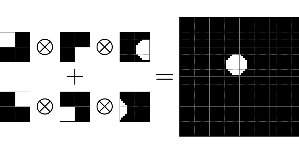
Figure 1: An illustration of DKN with $L=3$, $R=2$, $\boldsymbol{B}_{3}^{r},\boldsymbol{B}_{2}^{r}\in\mathbb{R}^{2\times 2}$, $\boldsymbol{B}_{1}^{r}\in\mathbb{R}^{4\times 4}$, $r=1,2$.

We call model (1), (2) and (3) Deep Kronecker Network as it resembles a fully convolutional network (FCN). In particular, the rank $R$ and factor number $L$ in DKN could be viewed as the width and depth of DKN, respectively. A detailed discussion between DKN and FCN is deferred to Section 4. Moreover, as in a neural network, the performance of DKN would also be affected by its structure, including depth, width and factor sizes. We defer to Section 4.3 for a detailed discussion on the network structure and its impact for performance.

Beyond matrix image, the DKN could be easily extended to tensor represented images. This would allow us to address general 3D and even higher order image data, e.g., MRI, fMRI, etc. We first need to introduce the definition of tensor Kronecker product (TKP):

Definition 2.1.

(Tensor Kronecker Product) Let $\mathbf{\mathcal{A}}\in\mathbb{R}^{d_{1}\times p_{1}\times q_{1}}$ and $\mathbf{\mathcal{B}}\in\mathbb{R}^{d_{2}\times p_{2}\times q_{2}}$ be two three-order tensor with entries denoted by $\mathbf{\mathcal{A}}_{i_{1},j_{1},k_{1}}$ and $\mathbf{\mathcal{B}}_{i_{2},j_{2},k_{2}}$, respectively. Then the tensor Kronecker product $\mathcal{C}=\mathbf{\mathcal{A}}\otimes\mathbf{\mathcal{B}}$ is defined by $\mathcal{C}_{[h_{1}h_{2}],[j_{1}j_{2}],[k_{1}k_{2}]}=\mathbf{\mathcal{A}}_{h_{1},j_{1},k_{1}}\mathbf{\mathcal{B}}_{h_{2},j_{2},k_{2}}$ for all possible values of $(h_{1},j_{1},k_{1})$ and $(h_{2},j_{2},k_{2})$.

For ease of presentation, Definition 2.1 is illustrated for three-order TKP. But it could be further extended to arbitrary higher order tensors. Given tensor images ${\bf{\mathcal{X}}}_{i}\in\mathbb{R}^{d\times p\times q}$, we may directly generalize matrix DKN (1) to (3) to its tensor version by replacing images $\boldsymbol{X}_{i}$, coefficients $\boldsymbol{C}$ and factors $\boldsymbol{B}_{l}^{r}$ with their tensor version ${\bf{\mathcal{X}}}_{i}\in\mathbb{R}^{d\times p\times q}$, $\mathcal{C}\in\mathbb{R}^{d\times p\times q}$ and $\mathbf{\mathcal{B}}^{r}_{l}\in\mathbb{R}^{d_{l}\times p_{l}\times q_{l}}$, respectively.

The DKN is designed for medical image analysis, where the sample size is usually limited, but images could be of high-resolution. Consider a simple case with images of size $(d,p,q)=(256,256,256)$. By setting $L=8$, $R=3$, and $(d_{1},p_{1},q_{1})=\cdots=(d_{8},p_{8},q_{8})=(2,2,2)$, the number of unknown parameters in DKN is reduced from $256^{3}=16,777,216$ to $2^{3}*8*3=192$. In general, the DKN is able to reduce the number of unknown parameters from $\prod_{l=1}^{L}d_{l}p_{l}q_{l}$ to $R\sum_{l=1}^{L}d_{l}p_{l}q_{l}$. Considering that sample size is only of hundreds or at most thousands in many medical image analyses, the dimension reduction achieved by DKN becomes more significant and critical.

In the literature, Kronecker product decomposition (KPD) has become a powerful tool for matrix approximation and dimension reduction. In particular, Kronecker product singular value decomposition (KPSVD) is referred to the problem of recovering $\boldsymbol{B}^{r}_{l}$, $l=1,2$, $r=1,\ldots,R$, from a given matrix $\boldsymbol{C}=\sum_{r=1}^{R}\bigotimes_{l=L}^{1}\boldsymbol{B}_{l}^{r}$. The KPSVD was mostly studied when $L=2$, e.g., Van Loan and Pitsianis, (1993); Cai et al., (2019), with rich theoretical and computational properties developed. While for the general case $L\geq 3$, the KPSVD becomes a much more difficult problem (Hackbusch et al.,, 2005) with rather limited literature. Batselier and Wong, (2017) considered the computation of KPSVD with $L\geq 3$ and proposed an algorithm to transform KPSVD to a tensor canonical polyadic decomposition (CPD) problem. Beyond KPSVD, KPD has also been studied in other contexts, e.g., correlation matrix estimation (Hafner et al.,, 2020), matrix autoregressive model (Chen et al.,, 2020), etc. Moreover, we note that there is a recent work uses Kronecker product for adaptive activation functions selection in neural network (Jagtap et al.,, 2022). This work shares a similar name to DKN, although the motivation and methodology are completely different.

Given model (1) to (3), we solve it with maximum likelihood estimation (MLE). To avoid duplication, we use the calligraphic tensor notation (such as ${\bf{\mathcal{X}}}_{i}$, $\mathcal{C}$, $\mathbf{\mathcal{B}}^{r}_{l}$, etc) to refer both tensors and matrices. Given $y_{i}$ and ${\bf{\mathcal{X}}}_{i}$, the negative likelihood function for factors $\left[\mathbf{\mathcal{B}}_{1}^{1},\ldots,\mathbf{\mathcal{B}}_{L}^{R}\right]$ is proportional to

$$\ell\left(\mathbf{\mathcal{B}}_{1}^{1},\ldots,\mathbf{\mathcal{B}}_{L}^{R}\right)=\sum_{i=1}^{n}\left\{\psi\left(\left\langle{\bf{\mathcal{X}}}_{i},\sum_{r=1}^{R}\bigotimes_{l=L}^{1}\mathbf{\mathcal{B}}_{l}^{r}\right\rangle\right)-y_{i}\ \left\langle{\bf{\mathcal{X}}}_{i},\sum_{r=1}^{R}\bigotimes_{l=L}^{1}\mathbf{\mathcal{B}}_{l}^{r}\right\rangle\right\}.$$ (4)

When the outcome $y_{i}$ is Gaussian distributed, the MLE reduces to standard least square

$$\ell\left(\mathbf{\mathcal{B}}_{1}^{1},\ldots,\mathbf{\mathcal{B}}^{R}_{L}\right)=\sum_{i=1}^{n}\left(y_{i}-\left\langle{\bf{\mathcal{X}}}_{i},\sum_{r=1}^{R}\bigotimes_{l=L}^{1}\mathbf{\mathcal{B}}_{l}^{r}\right\rangle\right)^{2}.$$ (5)

We demonstrate the computation of (4) and (5) in Section 3 below.

3 Computation

In this section, we propose an alternating minimization algorithm to solve DKN. The algorithm is illustrated for tensor images ${\bf{\mathcal{X}}}_{i}\in\mathbb{R}^{d\times p\times q}$. We shall first consider the computation of DKN with a fixed structure, i.e., given factor number $L$, rank $R$ and factor sizes $(d_{l},p_{l},q_{l})$, $l=1,\ldots,L$. The determination of network structure will be discussed in Section 4.3.

We a few more notations to get started. Let $\boldsymbol{b}^{r}_{l}=\text{vec}(\mathbf{\mathcal{B}}^{r}_{l})\in\mathbb{R}^{d_{l}p_{l}q_{l}}$ be the vectorization of $\mathbf{\mathcal{B}}^{r}_{l}$ for $l=1,\ldots,L$, $r=1,\ldots,R$. Let

$$\widebar{\boldsymbol{B}}_{l}=\left[\boldsymbol{b}^{1}_{l},\boldsymbol{b}^{2}_{l},\ldots,\boldsymbol{b}^{R}_{l}\right]\in\mathbb{R}^{(d_{l}p_{l}q_{l})\times R},\ \ \widebar{\boldsymbol{b}}_{l}=\text{vec}\left(\widebar{\boldsymbol{B}}_{l}\right)$$

be the combined matrix of $\boldsymbol{b}_{l}^{r}$ over different ranks and its vectorized version, respectively. Moreover, let $\mathbf{\mathcal{B}}_{(:l)}^{r}$ and $\mathbf{\mathcal{B}}_{(l:)}^{r}$ be the product of factors as below,

$$\mathbf{\mathcal{B}}_{(:l)}^{r}=\bigotimes_{k=L}^{l}\mathbf{\mathcal{B}}_{k}^{r},\ \ \mathbf{\mathcal{B}}_{(:L+1)}^{r}=1,\ \ \mathbf{\mathcal{B}}_{(l:)}^{r}=\bigotimes_{k=l}^{1}\mathbf{\mathcal{B}}_{k}^{r},\ \ \mathbf{\mathcal{B}}_{(0:)}^{r}=1,\ \ l=1,\ldots,L.$$

Further let $\boldsymbol{b}_{(:l)}^{r}$ and $\boldsymbol{b}_{(l:)}^{r}$ be the vectorized version of $\mathbf{\mathcal{B}}_{(:l)}^{r}$ and $\mathbf{\mathcal{B}}_{(l:)}^{r}$, respectively,

$$\boldsymbol{b}_{(:l)}^{r}=\text{vec}\left(\mathbf{\mathcal{B}}_{(:l)}^{r}\right),\ \ \ \boldsymbol{b}_{(l:)}^{r}=\text{vec}\left(\mathbf{\mathcal{B}}_{(l:)}^{r}\right),\ \ \ l=1,\ldots,L.$$

Finally, define the combined matrices of $\boldsymbol{b}_{(:l)}^{r}$ and $\boldsymbol{b}_{(l:)}^{r}$ over different ranks

$$\widebar{\boldsymbol{B}}_{(:l)} = \left[\boldsymbol{b}^{1}_{(:l)},\boldsymbol{b}^{2}_{(:l)},\ldots,\boldsymbol{b}^{R}_{(:l)}\right],\ \ \ \widebar{\boldsymbol{b}}_{(:l)}=\text{vec}\left(\widebar{\boldsymbol{B}}_{(:l)}\right),$$

$$\widebar{\boldsymbol{B}}_{(l:)} = \left[\boldsymbol{b}^{1}_{(l:)},\boldsymbol{b}^{2}_{(l:)},\ldots,\boldsymbol{b}^{R}_{(l:)}\right],\ \ \ \widebar{\boldsymbol{b}}_{(l:)}=\text{vec}\left(\widebar{\boldsymbol{B}}_{(l:)}\right).$$

Now we introduce a tensor reshaping operator. Let $\mathcal{C}$ be any tensor of dimension $d\times p\times q$, and $d^{\prime}$, $p^{\prime}$, and $q^{\prime}$ be any integer that could be divided by $d$, $p$, and $q$ respectively. Let $(d^{\prime\prime},p^{\prime\prime},q^{\prime\prime})=(d/d^{\prime},p/p^{\prime},q/q^{\prime})$. Define the operator $\mathcal{R}:\mathbb{R}^{d\times p\times q}\rightarrow\mathbb{R}^{(d^{\prime}p^{\prime}q^{\prime})\times(d^{\prime\prime}p^{\prime\prime}q^{\prime\prime})}$ be a mapping from $\mathcal{C}$ to

$$\mathcal{R}_{(d^{\prime},p^{\prime},q^{\prime})}(\mathcal{C})= \Big{[}\text{vec}(\mathcal{C}_{1,1,1}^{d^{\prime\prime},p^{\prime\prime},q^{\prime\prime}}),\ldots,\text{vec}(\mathcal{C}_{1,1,q^{\prime}}^{d^{\prime\prime},p^{\prime\prime},q^{\prime\prime}}),\ldots,\text{vec}(\mathcal{C}_{1,p^{\prime},1}^{d^{\prime\prime},p^{\prime\prime},q^{\prime\prime}}),\ldots,\text{vec}(\mathcal{C}_{1,p^{\prime},q^{\prime}}^{d^{\prime\prime},p^{\prime\prime},q^{\prime\prime}}),\ldots,$$

$$\ \ \text{vec}(\mathcal{C}_{d^{\prime},1,1}^{d^{\prime\prime},p^{\prime\prime},q^{\prime\prime}}),\ldots,\text{vec}(\mathcal{C}_{d^{\prime},1,q^{\prime}}^{d^{\prime\prime},p^{\prime\prime},q^{\prime\prime}}),\ldots,\text{vec}(\mathcal{C}_{d^{\prime},p^{\prime},1}^{d^{\prime\prime},p^{\prime\prime},q^{\prime\prime}}),\ldots,\text{vec}(\mathcal{C}_{d^{\prime},p^{\prime},q^{\prime}}^{d^{\prime\prime},p^{\prime\prime},q^{\prime\prime}})\Big{]}^{\top}.$$

where $\mathcal{C}_{j,k,l}^{d^{\prime\prime},p^{\prime\prime},q^{\prime\prime}}$ is the $(j,k,l)$-th block of $\mathcal{C}$ of size $d^{\prime\prime}\times p^{\prime\prime}\times q^{\prime\prime}$. A key property of the operator $\mathcal{R}$ is that for any tensor Kronecker product $\mathbf{\mathcal{A}}\otimes\mathbf{\mathcal{B}}$,

$$\mathcal{R}(\mathbf{\mathcal{A}}\otimes\mathbf{\mathcal{B}})=\text{vec}(\mathbf{\mathcal{A}})\left[\text{vec}(\mathbf{\mathcal{B}})\right]^{\top}.$$ (6)

Given above definitions, we have the following Proposition.

Proposition 1.

Let ${\widetilde{\boldsymbol{X}}}_{i}\left(\boldsymbol{b}^{r}_{(:l+1)},\ \boldsymbol{b}^{r}_{(l-1:)}\right)$ be a function of $\boldsymbol{b}^{r}_{(:l+1)}$ and $\boldsymbol{b}^{r}_{(l-1:)}$,

$${\widetilde{\boldsymbol{X}}}_{i}\left(\boldsymbol{b}^{r}_{(:l+1)},\ \boldsymbol{b}^{r}_{(l-1:)}\right)$$

$$= \mathcal{R}_{(d_{l},p_{l},q_{l})}\left(\text{vec}^{-1}_{\left(d_{(l:)},p_{(l:)},q_{(l:)}\right)}\left(\left[\boldsymbol{b}^{r}_{(:l+1)}\right]^{\top}\mathcal{R}_{\left(d_{(:l+1)},p_{(:l+1)},q_{(:l+1)}\right)}(\boldsymbol{X}_{i})\right)\right)\boldsymbol{b}^{r}_{(l-1:)}.$$

where we denote $d_{(l:)}=\prod_{j=l}^{1}d_{j}$, $d_{(:l+1)}=\prod_{j=l+1}^{L}d_{j}$. The same notations are also used for $p$ and $q$. Furthermore, let $\widebar{\boldsymbol{X}}_{i}(\widebar{\boldsymbol{b}}_{(:l+1)},\ \widebar{\boldsymbol{b}}_{(l-1:)})$ be a function of $\widebar{\boldsymbol{b}}_{(:l+1)}$ and $\widebar{\boldsymbol{b}}_{(l-1:)}$,

$$\widebar{\boldsymbol{X}}_{i}\left(\widebar{\boldsymbol{b}}_{(:l+1)},\ \widebar{\boldsymbol{b}}_{(l-1:)}\right)=\left[{\widetilde{\boldsymbol{X}}}_{i}\left(\boldsymbol{b}^{1}_{(:l+1)},\ \boldsymbol{b}^{1}_{(l-1:)}\right),\ldots,{\widetilde{\boldsymbol{X}}}_{i}\left(\boldsymbol{b}^{R}_{(:l+1)},\ \boldsymbol{b}^{R}_{(l-1:)}\right)\right].$$

Then we have

$$\left\langle{\bf{\mathcal{X}}}_{i},\sum_{r=1}^{R}\bigotimes_{l=L}^{1}\mathbf{\mathcal{B}}_{l}^{r}\right\rangle=\left[\text{vec}\left(\widebar{\boldsymbol{X}}_{i}\left(\widebar{\boldsymbol{b}}_{(:l+1)},\ \widebar{\boldsymbol{b}}_{(l-1:)}\right)\right)\right]^{\top}\widebar{\boldsymbol{b}}_{l}.$$ (7)

As a consequence, the loss function $\ell\left(\mathbf{\mathcal{B}}^{1}_{1},\ldots,\mathbf{\mathcal{B}}^{R}_{L}\right)$ could be written as

$$\ell\left(\widebar{\boldsymbol{b}}_{l},\ \widebar{\boldsymbol{b}}_{(:l+1)},\ \widebar{\boldsymbol{b}}_{(l-1:)}\right)$$ (8)

$$= \sum_{i=1}^{n}\psi\Big{(}\Big{[}\text{vec}\Big{(}\widebar{\boldsymbol{X}}_{i}\left(\widebar{\boldsymbol{b}}_{(:l+1)},\widebar{\boldsymbol{b}}_{(l-1:)}\right)\Big{)}\Big{]}^{\top}\widebar{\boldsymbol{b}}_{l}\Big{)}-y_{i}\Big{[}\text{vec}\Big{(}\widebar{\boldsymbol{X}}_{i}\left(\widebar{\boldsymbol{b}}_{(:l+1)},\widebar{\boldsymbol{b}}_{(l-1:)}\right)\Big{)}\Big{]}^{\top}\widebar{\boldsymbol{b}}_{l}.$$ (9)

That is to say, given $\widebar{\boldsymbol{b}}_{(:l+1)}$ and $\widebar{\boldsymbol{b}}_{(l-1:)}$, the new $\widehat{\widebar{\boldsymbol{b}}}_{l}$ can be updated by standard GLM estimation. With updated $\widehat{\widebar{\boldsymbol{b}}}_{l}$ , we further have new

$$\widehat{\widebar{\boldsymbol{B}}}_{l}=\text{vec}_{(d_{l}p_{l}q_{l},R)}^{-1}\left(\widehat{\widebar{\boldsymbol{b}}}_{l}\right),$$ (10)

$${\widehat{\boldsymbol{b}}}^{r}_{l}=\left[\widehat{\widebar{\boldsymbol{B}}}_{l}\right]_{r,\cdot},\ \text{the r-th column of }\widehat{\widebar{\boldsymbol{B}}}_{l},$$ (11)

$$\widehat{\mathbf{\mathcal{B}}}^{r}_{l}=\text{vec}_{(d_{l},p_{l},q_{l})}^{-1}({\widehat{\boldsymbol{b}}}^{r}_{l}),$$ (12)

$${\widehat{\boldsymbol{b}}}^{r}_{(l:)}=\text{vec}\left(\widehat{\mathbf{\mathcal{B}}}^{r}_{l}\otimes\left[\widehat{\mathbf{\mathcal{B}}}^{r}_{(l-1:)}\right]^{(old)}\right),$$ (13)

$$\widehat{\widebar{\boldsymbol{B}}}_{(l:)}=\left[{\widehat{\boldsymbol{b}}}^{1}_{(:l)},{\widehat{\boldsymbol{b}}}^{2}_{(:l)},\ldots,{\widehat{\boldsymbol{b}}}^{R}_{(:l)}\right],$$ (14)

$$\widehat{\widebar{\boldsymbol{b}}}_{(l:)}=\text{vec}\left(\widehat{\widebar{\boldsymbol{B}}}_{(l:)}\right).$$ (15)

Proposition 1 suggests that the DKN could be solved by an alternating minimization algorithm with $\widebar{\boldsymbol{b}}_{1},\ldots,\widebar{\boldsymbol{b}}_{L}$ updated iteratively. To implement the alternating minimization algorithm, the initializations of ${\widehat{\boldsymbol{b}}}_{(:2)},{\widehat{\boldsymbol{b}}}_{(:3)},\ldots,{\widehat{\boldsymbol{b}}}_{(:L)}$ are needed. They could be obtained by singular value decompositions as below:

$$\widehat{\widebar{\boldsymbol{b}}}_{(:l)}^{(0)}=\text{vec}\left(\widehat{\widebar{\boldsymbol{B}}}_{(:l)}^{(0)}\right),\ \ \ \widehat{\widebar{\boldsymbol{B}}}_{(:l)}^{(0)}=\left(\left[{\widehat{\boldsymbol{b}}}^{1}_{(l:)}\right]^{(0)},\left[{\widehat{\boldsymbol{b}}}^{2}_{(l:)}\right]^{(0)},\ldots,\left[{\widehat{\boldsymbol{b}}}^{R}_{(l:)}\right]^{(0)}\right),$$ (16)

$$\left[{\widehat{\boldsymbol{b}}}_{(:l)}^{r}\right]^{(0)}=\text{SVD}_{u,r}\left(\sum_{i=1}^{n}y_{i}\mathcal{R}_{\left(d_{(:l)},p_{(:l)},q_{(:l)}\right)}({\bf{\mathcal{X}}}_{i})\right),\ \ l=2,3,\ldots,L,$$ (17)

where $\text{SVD}_{u,r}(\boldsymbol{X})$ denote the $r$-th top left singular vector of $\boldsymbol{X}$. We summarize the alternating minimization algorithm in Algorithm 1 below.

Algorithm 1.

Alternating Minimization Algorithm for DKN

Input: $\boldsymbol{y}_{i}$ and ${\bf{\mathcal{X}}}_{i}$, $i=1,\ldots,n$.

Initialization: $\left[\widehat{\widebar{\boldsymbol{b}}}_{(:l)}^{r}\right]^{(0)}$ is obtained by (16).

For $t$ in $0,1,\ldots,T-1$

For $l$ in $1,2,\ldots,L$

$\widehat{\widebar{\boldsymbol{b}}}_{l}^{(t+1)}\leftarrow\operatorname{argmin}\displaylimits_{\widebar{\boldsymbol{b}}_{l}}\ell\left(\widebar{\boldsymbol{b}}_{l},\ \widehat{\widebar{\boldsymbol{b}}}_{(:l+1)}^{(t)},\ \widehat{\widebar{\boldsymbol{b}}}_{(l-1:)}^{(t+1)}\right)$, where $\ell(\cdot,\cdot,\cdot)$ defined in (8).

$\widehat{\widebar{\boldsymbol{b}}}_{(l:)}^{(t+1)}$ updated by (10).

For $l$ in $L,(L-1),\ldots,1$

$\widehat{\widebar{\boldsymbol{B}}}_{l}^{(t+1)}\leftarrow\text{vec}_{(d_{l}p_{l}q_{l},R)}^{-1}\left(\widehat{\widebar{\boldsymbol{b}}}_{l}^{(t+1)}\right)$;

$\left[{\widehat{\boldsymbol{b}}}^{r}_{l}\right]^{(t+1)}\leftarrow\left[\widehat{\widebar{\boldsymbol{B}}}_{l}^{(t+1)}\right]_{r,\cdot}$

$\left[\widehat{\mathbf{\mathcal{B}}}^{r}_{l}\right]^{(t+1)}\leftarrow\text{vec}_{(d_{l},p_{l},q_{l})}^{-1}\left(\left[{\widehat{\boldsymbol{b}}}^{r}_{l}\right]^{(t+1)}\right)$

$\left[\widehat{\mathbf{\mathcal{B}}}^{r}_{(:l)}\right]^{(t+1)}\leftarrow\left[\widehat{\mathbf{\mathcal{B}}}^{r}_{(:l+1)}\right]^{(t+1)}\otimes\left[\widehat{\mathbf{\mathcal{B}}}^{r}_{l}\right]^{(t+1)}$;

$\left[{\widehat{\boldsymbol{b}}}^{r}_{(:l)}\right]^{(t+1)}\leftarrow\text{vec}\left(\left[\widehat{\mathbf{\mathcal{B}}}^{r}_{(:l)}\right]^{(t+1)}\right)$

$\widehat{\widebar{\boldsymbol{b}}}_{(:l)}^{(t+1)}\leftarrow\text{vec}\left(\left[{\widehat{\boldsymbol{b}}}^{1}_{(:l)}\right]^{(t+1)},\left[{\widehat{\boldsymbol{b}}}^{2}_{(:l)}\right]^{(t+1)},\ldots,\left[{\widehat{\boldsymbol{b}}}^{R}_{(:l)}\right]^{(t+1)}\right)$;

Output $\widehat{\widebar{\boldsymbol{b}}}_{1}^{(T)},\ldots,\widehat{\widebar{\boldsymbol{b}}}_{L}^{(T)}$.

4 Convolutional DKN, nonlinear DKN and FCN

4.1 DKN in a Convolutional Form

We name model (1) to (3) Deep Kronecker Network because it resembles a $L$-layer fully convolutional network (FCN). To demonstrate this connection, we first introduce a non-overlapping convolutional operator. For given tensors ${\bf{\mathcal{X}}}\in\mathbb{R}^{d_{0}\times p_{0}\times q_{0}}$ and $\mathbf{\mathcal{B}}\in\mathbb{R}^{d^{\prime}\times p^{\prime}\times q^{\prime}}$, define the non-overlapping convolution between ${\bf{\mathcal{X}}}$ and $\mathbf{\mathcal{B}}$ as

$${\bf{\mathcal{X}}}*\mathbf{\mathcal{B}}\in\mathbb{R}^{d^{\prime\prime}\times p^{\prime\prime}\times q^{\prime\prime}},\ \ \ d^{\prime\prime}=d_{0}/d^{\prime},\ \ p^{\prime\prime}=p_{0}/p^{\prime},\ \ q^{\prime\prime}=q_{0}/q^{\prime}$$

with the $(h,j,k)$-th component being

$$({\bf{\mathcal{X}}}*\mathbf{\mathcal{B}})_{h,j,k}=\left\langle{\bf{\mathcal{X}}}_{h,j,k}^{d^{\prime}\times p^{\prime}\times q^{\prime}},\mathbf{\mathcal{B}}\right\rangle,\ \ 1\leq h\leq d^{\prime\prime},\ 1\leq j\leq p^{\prime\prime},\ 1\leq k\leq q^{\prime\prime}.$$

Here ${\bf{\mathcal{X}}}_{h,j,k}^{d^{\prime}\times p^{\prime}\times q^{\prime}}$ is the $(h,j,k)$-th block of ${\bf{\mathcal{X}}}$ and is of size $d^{\prime}\times p^{\prime}\times q^{\prime}$. Building on this operator, the following theorem connects DKN and FCN:

Theorem 4.1.

For $i=1,\ldots,n$, the Deep Kronecker product model

$$g\left(\mathbb{E}(y_{i})\right)=\left\langle{\bf{\mathcal{X}}}_{i},\sum_{r=1}^{R}\bigotimes_{l=L}^{1}\mathbf{\mathcal{B}}_{l}^{r}\right\rangle$$

is equivalent to the following convolutional form

$$g\left(\mathbb{E}(y_{i})\right)=\sum_{r=1}^{R}{\bf{\mathcal{X}}}_{i}*\mathbf{\mathcal{B}}^{r}_{1}*\mathbf{\mathcal{B}}^{r}_{2}*\cdots*\mathbf{\mathcal{B}}^{r}_{L-1}*\mathbf{\mathcal{B}}^{r}_{L}.$$

By Theorem 4.1, the response $y_{i}$ in DKN is in fact modeled by a summation of consecutive convolutions between input image ${\bf{\mathcal{X}}}_{i}$ and factors $\mathbf{\mathcal{B}}^{r}_{l}$. In other words, the DKN could be viewed as a FCN, a network only of convolutional layers. The FCN has been studied in the deep learning literature for different computer vision tasks, such as semantic segmentation (Long et al.,, 2015), image segmentation (Ronneberger et al.,, 2015), etc.

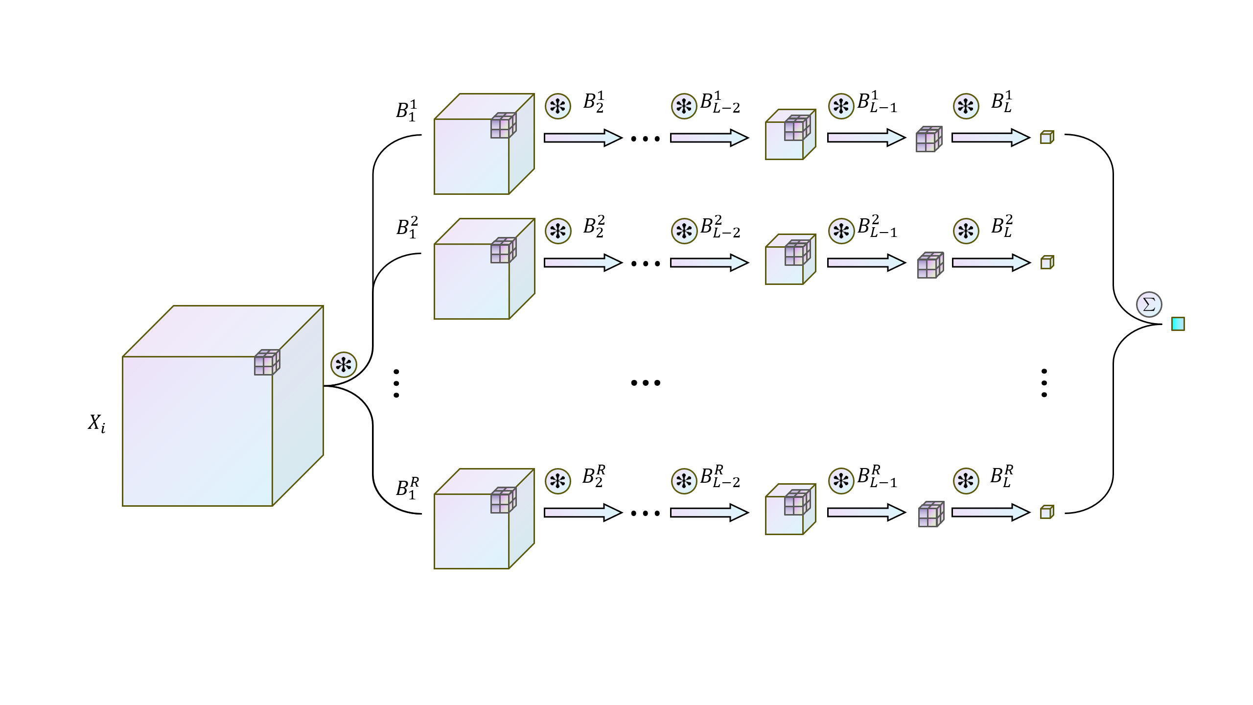
Figure 2: An illustration of DKN in a convolutional form.

More specifically, we may view $L$ as the depth of a DKN, $R$ as the width, and the Kronecker factors $\mathbf{\mathcal{B}}_{l}^{r}$ as the convolution filters. While the activation functions in DKN is taken as an identity function. If we further change the identity activation to a nonlinear function, the DKN could be generalized to its nonlinear version. We refer to such a DKN nonlinear DKN. The discussion on nonlinear DKN is deferred to Section 4.2. Figure 2 illustrates the DKN in a convolutional form.

On the other hand, the convolutions in a DKN have no overlaps with each other, i.e., the stride sizes are equal to the filter sizes. Such a design has at least two advantages. First, it is the key for DKN to achieve maximized dimension reduction, which is very necessary in medical imaging analysis as discussed above. Second, the non-overlapping structure allow us to explicitly write down the coefficients matrix $\mathcal{C}$. With an explicit coefficients matrix, we are able to locate the regions/areas that are most influential to the outcome and have the desired model interpretability.

4.2 Nonlinear DKN and Fully Convolutional Network

By including the nonlinear activation functions, the DKN could be generalized to its nonlinear version:

$$g\left(\mathbb{E}(y_{i})\right)=\sum_{r=1}^{R}h\left(\cdots h\left(h({\bf{\mathcal{X}}}_{i}*\mathbf{\mathcal{B}}^{r}_{1})*\mathbf{\mathcal{B}}^{r}_{2}\right)\cdots*\mathbf{\mathcal{B}}^{r}_{L-1}\right)*\mathbf{\mathcal{B}}^{r}_{L},$$ (18)

where $h(\cdot)$ is certain nonlinear activation functions, for example, ReLU, $h(\mathbf{\mathcal{B}})=(\mathbf{\mathcal{B}}+|\mathbf{\mathcal{B}}|)/2$. Given the nonlinear form (18), the resulted objective function becomes

$$\ell\left(\mathbf{\mathcal{B}}_{1}^{1},\ldots,\mathbf{\mathcal{B}}_{L}^{R}\right) = \sum_{i=1}^{n}\Big{\{}\psi\big{(}\sum_{r=1}^{R}h\left(\cdots h\left(h({\bf{\mathcal{X}}}_{i}*\mathbf{\mathcal{B}}^{r}_{1})*\mathbf{\mathcal{B}}^{r}_{2}\right)\cdots*\mathbf{\mathcal{B}}^{r}_{L-1}\right)*\mathbf{\mathcal{B}}^{r}_{L},\big{)}$$ (20)

$$\ \ \ \ \ -\ y_{i}\sum_{r=1}^{R}h\left(\cdots h\left(h({\bf{\mathcal{X}}}_{i}*\mathbf{\mathcal{B}}^{r}_{1})*\mathbf{\mathcal{B}}^{r}_{2}\right)\cdots*\mathbf{\mathcal{B}}^{r}_{L-1}\right)*\mathbf{\mathcal{B}}^{r}_{L}\Big{\}}.$$

Here we omit the discussion on the computation of (20) as it could be solved easily by standard deep learning tools, such as Pytorch.

We shall also note that the pooling layer, such as max pooling or average pooling, is usually imposed in CNN. However, it is not needed in DKN. The pooling layer is commonly used in CNN to reduce the size of feature maps. While in DKN, the non-overlap design has already enabled DKN to achieve maximized dimension reduction. From another perspective, the non-overlapping convolution could also be regraded as an adaptive (average) pooling with the kernel weights to be learned. Therefore, the DKN is able to achieve feature extraction and dimension reduction simultaneously.

4.3 Network Structure: Depth vs Width

In a convolutional neural network, or general deep neural network, the structure usually need to be carefully tuned in order to achieve the optimal prediction power. In particular, how the depth and width of a neural network would affect its prediction power has been intensively studied in the literature, to list a few, Raghu et al., (2017); Lu et al., (2017); Tan and Le, (2019). Similarly, it is also of a concern in DKN how to find an optimal structure. In this subsection, we provide a general guidance on the determination of DKN structure.

To implement a DKN, the depth $L$, width $R$ and the filter sizes $\mathbf{\mathcal{B}}_{l}^{r}$, i.e., $(d_{l},p_{l},q_{l})$, need to be determined. Although they could all be treated as tuning parameters, we argue that it is not necessary to tune them all.

First, we note that for any given $L$ and $(d_{l},p_{l},q_{l})$, there exists a corresponding $R$ such that any tensor of size $\left(\prod_{l=1}^{L}d_{l},\ \prod_{l=1}^{L}p_{l},\ \prod_{l=1}^{L}q_{l}\right)$ could be approximated. Such a result could be seen by relating KPD with CP decomposition. See Lemma 5.1 below. In other words, it is not necessary to tune the depth $L$ and filter sizes $(d_{l},p_{l},q_{l})$ carefully.

Second, a deeper DKN is usually preferred. Recall that DKN is designed for image analysis under limited sample sizes. A deepest DKN allows us to achieve maximized dimension reduction. For example, suppose the images of concern are of size $(d,p,q)=(256,256,256)$. If we consider a 8-layer DKN with all the filters are $2\times 2\times 2$, then the total number of unknown parameters in a rank-R DKN is $R*64(=2^{3}*8)$. As a comparison, the unknown parameter number in 2-layer, rank-$R$, filters size $(16,16,16)$ DKN is $R*8192(=16^{3}*2)$. Certainly, a larger $R$ is possibly needed in a deeper DKN in order to achieve a better expressive power. But still, the benefit of depth is tremendous. In our simulation and real data analysis later, we stick to the deepest possible DKN.

Third, given $L$ and $(d_{l},p_{l},q_{l})$, it is possible to design an information criterion to choose the rank $R$. For example, we may minimize the Bayesian Information Criterion (BIC)

$$\text{BIC}(R)=2\ell\left(\widehat{\mathbf{\mathcal{B}}}_{1}^{1},\ldots,\widehat{\mathbf{\mathcal{B}}}_{L}^{R}\right)+\left(R\sum_{l=1}^{L}d_{l}p_{l}q_{l}\right)\log n$$ (21)

In practice, we find that a relatively low rank model (e.g., $R=1,2,3$) in many cases would already produce desired estimation accuracy and prediction power. Therefore, we usually suggest to implement DKN from low-rank models.

5 DKN and Tensor Regression

In the tensor regression (TR) framework (Zhou et al.,, 2013), the coefficients are assumed to follow a CANDECOMP/PARAFAC (CP) low-rank decompositions. In this section, we show that the DKN is highly connected to the TR.

To get started, we first recall the Definition 2.1 for tensor KPD. Suppose a tensor $\mathcal{C}$ could be written into a Kronecker product of $L$ smaller tensors $\mathcal{C}=\bigotimes_{l=L}^{1}\mathbf{\mathcal{B}}_{l}$. Then the entries of $\mathcal{C}$ is characterized by

$$\mathcal{C}_{{[h_{1}\cdots h_{L}],[j_{1}\cdots j_{L}],[k_{1}\cdots k_{L}]}}=\prod_{l=1}^{L}[\mathbf{\mathcal{B}}_{l}]_{h_{l},j_{l},k_{l}}.$$

Now let $\mathcal{T}:\mathbb{R}^{d\times p\times q}\rightarrow\mathbb{R}^{(d_{1}p_{1}q_{1})\times(d_{2}p_{2}q_{2})\times\cdots\times(d_{L}p_{L}q_{L})}$ be a reshaping operator from tensor $\mathcal{C}$ to an $L$-order tensor $\mathcal{T}(\mathcal{C})$ with the entries characterized as below:

$$\left[\mathcal{T}(\mathcal{C})\right]_{{[h_{1}j_{1}k_{1}],\ldots,[h_{L}j_{L}k_{L}]}}=\mathcal{C}_{{[h_{1}\cdots h_{L}],[j_{1}\cdots j_{L}],[k_{1}\cdots k_{L}]}}.$$

Given this transformation, Batselier and Wong, (2017) provides an interesting connection between the KPD and CP decomposition (CPD).

Lemma 5.1.

(Batselier and Wong,, 2017) Given a tensor $\mathcal{C}\in\mathbb{R}^{d\times p\times q}$, if $\mathcal{C}=\sum_{r=1}^{R}\bigotimes_{l=L}^{1}\mathbf{\mathcal{B}}_{l}^{r}$. then we have $\mathcal{T}(\mathcal{C})=\sum_{r=1}^{R}\boldsymbol{b}^{r}_{L}\circ\cdots\circ\boldsymbol{b}^{r}_{1}$, where $\boldsymbol{b}^{r}_{l}=\text{vec}(\mathbf{\mathcal{B}}^{r}_{l})$ for all  $l=1,\ldots,L$ and $r=1,\ldots,R$.

As the reshaping operator $\mathcal{T}(\cdot)$ is one-to-one and any tensor could be approximated by CPD, Lemma 5.1 allows us to claim that KPD (3) is also able to approximate arbitrary tensors with a sufficiently large rank $R$. On the other hand, the equivalence also allows us to derive the conditions under which the KPD is identifiable, which will be deferred to Section 6.1. Furthermore, we are able to build the following connections between DKN and tensor regression.

Theorem 5.2.

Let $\widetilde{\bf{\mathcal{X}}}_{i}=\mathcal{T}({\bf{\mathcal{X}}}_{i})$ be the reshaped images. Then the DKN model

$$g\left(\mathbb{E}(y_{i})\right)=\left\langle{\bf{\mathcal{X}}}_{i},\sum_{r=1}^{R}\bigotimes_{l=L}^{1}\mathbf{\mathcal{B}}_{l}^{r}\right\rangle$$

is equivalent to the tensor regression with reshaped images $\widetilde{\bf{\mathcal{X}}}_{i}$:

$$g\left(\mathbb{E}(y_{i})\right)=\left\langle\widetilde{\bf{\mathcal{X}}}_{i},\sum_{r=1}^{R}\boldsymbol{b}^{r}_{L}\circ\cdots\circ\boldsymbol{b}^{r}_{1}\right\rangle,$$

in the sense that $\boldsymbol{b}^{r}_{l}=\text{vec}\left(\mathbf{\mathcal{B}}^{r}_{l}\right)$ hold for all  $l=1,\ldots,L$ and $r=1,\ldots,R$.

Remark 5.3.

By Theorem 5.2, we further have that the problem

$$(\widehat{\bf{\mathcal{B}}}_{1}^{1},\ldots,\widehat{\bf{\mathcal{B}}}^{R}_{L})\in\operatorname{argmin}\displaylimits_{\mathbf{\mathcal{B}}^{1}_{1},\ldots,\mathbf{\mathcal{B}}^{R}_{L}}\ \frac{1}{n}\sum_{i=1}^{n}\left(y_{i}-\left\langle{\bf{\mathcal{X}}}_{i},\sum_{r=1}^{R}\bigotimes_{l=L}^{1}\mathbf{\mathcal{B}}_{l}^{r}\right\rangle\right)^{2}$$ (22)

is equivalent to the tensor regression problem

$$({\widehat{\boldsymbol{b}}}_{1}^{1},\ldots,{\widehat{\boldsymbol{b}}}^{R}_{L})\in\min_{\boldsymbol{b}^{1}_{1},\ldots,\boldsymbol{b}^{R}_{L}}\ \frac{1}{n}\sum_{i=1}^{n}\left(y_{i}-\left\langle\widetilde{\bf{\mathcal{X}}}_{i},\sum_{r=1}^{R}\boldsymbol{b}^{r}_{L}\circ\cdots\circ\boldsymbol{b}^{r}_{1}\right\rangle\right)^{2}$$ (23)

in the sense that all the solutions are one-to-one:

$${\widehat{\boldsymbol{b}}}^{r}_{l}=\text{vec}\left(\widehat{\bf{\mathcal{B}}}^{r}_{l}\right)$$

for all  $l=1,\ldots,L$ and $r=1,\ldots,R$. In fact, the alternating minimization algorithm in Section 3 is also equivalent to the block relaxation algorithm in Zhou et al., (2013) applied on the transformed tensors $\widetilde{\bf{\mathcal{X}}}_{i}$.

Although the DKN and TR is highly connected to each other, the philosophies behind are significantly different. The TR is designed for general tensor represented predictors, while the DKN is specifically for image data. By utilizing the Kronecker product, the DKN imposes a latent blockwise smoothness structure for the coefficients. Such a smoothness structure is particularly suitable for image analysis, as it allows us to capture the significant regions in the images and at the same time provide better interpretation. However, for other types of tensor/matrix represented predictors, such a structure may not be desired.

6 Theoretical Analysis

In this section, we provide theoretical results for DKN. Specifically, we in Section 6.1 show that the KPD (1) is identifiable under mild conditions. In Section 6.2 we prove that the alternating minimization algorithm is able to guarantee the DKN to converge to the truth even if the objective function is highly nonconvex.

6.1 Identifiability conditions for $\mathbf{\mathcal{B}}^{r}_{l}$

In general, when the structure of DKN, including the depth $L$, width $R$ and factor sizes $(d_{l},p_{l},q_{l})$, $l=1,\ldots,L$, is unknown, the unknown tensors $\mathbf{\mathcal{B}}^{r}_{l}$ are not identifiable. Therefore, we here focus on the case that the structure of DKN is given and derive the conditions under which the $\mathbf{\mathcal{B}}^{r}_{l}$ are identifiable.

Before discussing the identifiability condition, we shall first realize two elementary indeterminacies of KPD, namely scaling and permutation. If a tensor $\mathcal{C}$ can be represented by KPD (3) with target tensors $\mathbf{\mathcal{B}}^{r}_{l}$, we use the notation $\mathcal{C}=[\![\mathbf{\mathcal{B}}^{r}_{l}]\!]$ to refer this decomposition. Meanwhile, recall the notation $\boldsymbol{b}^{r}_{l}=\text{vec}(\mathbf{\mathcal{B}}^{r}_{l})$ and $\widebar{\boldsymbol{B}}_{l}=\left[\boldsymbol{b}^{1}_{l},\boldsymbol{b}^{2}_{l},\ldots,\boldsymbol{b}^{R}_{l}\right]$. So we also use $\mathcal{C}=[\![\bar{\boldsymbol{B}}_{1},\ldots,\bar{\boldsymbol{B}}_{L}]\!]$ to refer the same decomposition. The scaling indeterminacy states that $\mathcal{C}=[\![\mathbf{\mathcal{B}}^{r}_{l}]\!]=[\![\mathbf{\mathcal{B}}^{r}_{l}\gamma_{l}^{r}]\!]$, when $\prod_{l=1}^{L}\gamma_{l}^{r}=1$, for all $r=1,\ldots,R$. The permutation indeterminacy states that $\mathcal{C}=[\![\bar{\boldsymbol{B}}_{1},\ldots,\bar{\boldsymbol{B}}_{L}]\!]=[\![\bar{\boldsymbol{B}}_{1}\Omega,\ldots,\bar{\boldsymbol{B}}_{L}\Omega]\!]$, where $\boldsymbol{\Omega}$ is certain permutation matrix. To avoid the two indeterminacies, we impose the following constraints. We first let $\lambda_{r}=\prod_{l=1}^{L}\|\mathbf{\mathcal{B}}^{r}_{l}\|_{F}$ to denote the $r$-th “Kronecker eigenvalue (KE)” in KPD. To address the scaling indeterminacy, we fix $\|\mathbf{\mathcal{B}}_{1}^{r}\|_{F}=\lambda_{r}$ and $\|\mathbf{\mathcal{B}}^{r}_{l}\|_{F}=1$ for $l=2,\ldots,L$ across all the terms $r=1,\ldots,R$. To address the permutation indeterminacy, we permute $\mathbf{\mathcal{B}}^{r}_{l}$ such that $\lambda_{1}\geq\cdots\geq\lambda_{R}$ for all the layers $l=1,\ldots,L$.

Now we are ready to state the sufficient and necessary conditions for identification.

Theorem 6.1.

Suppose $\mathcal{C}$ has a KPD form $\mathcal{C}=\sum_{r=1}^{R}\bigotimes_{l=L}^{1}\mathbf{\mathcal{B}}_{l}^{r}$. Suppose that the configuration of DKN, including the depth $L$, width $R$ and block sizes $(d_{l},p_{l},q_{l})$, $l=1,\ldots,L$, are correctly specified. Let $\boldsymbol{b}^{r}_{l}=\text{vec}(\mathbf{\mathcal{B}}^{r}_{l})$ and $\widebar{\boldsymbol{B}}_{l}=\left[\boldsymbol{b}^{1}_{l},\boldsymbol{b}^{2}_{l},\ldots,\boldsymbol{b}^{R}_{l}\right]$. Then:

• (Sufficiency) The KPD is unique up to scaling and permutation if

  $$\sum_{l=1}^{L}K\left(\widebar{\boldsymbol{B}}_{l}\right)\geq 2R+L-1$$

  where $K(\boldsymbol{M})$ is the $K$-rank of a matrix $\boldsymbol{M}$, i.e., the maximum value K such that any K columns of $\boldsymbol{M}$ are linearly independent.

• (Necessity) If the KPD is unique up to scaling and permutation, then

  $$\min_{l=1,\cdots L}\left\{\prod_{l^{\prime}\neq l}\hbox{\rm rank}\left(\widebar{\boldsymbol{B}}_{l}\right)\right\}\geq R$$

Remark 6.2.

When $L=2$, the KPD could be transformed into singular value decomposition (SVD) by Lemma 5.1. So we immediately have the sufficient and necessary condition for KPD: $\left\langle\mathbf{\mathcal{B}}^{r_{1}}_{1},\mathbf{\mathcal{B}}^{r_{2}}_{1}\right\rangle=0$, $\left\langle\mathbf{\mathcal{B}}^{r_{1}}_{2},\mathbf{\mathcal{B}}^{r_{2}}_{2}\right\rangle=0$, $\forall r_{1}\neq r_{2}$. The KPD under $L=2$ has been intensively studied in the literature and it was usually named as Kronecker product singular value decomposition (KPSVD). We refer to Van Loan and Pitsianis, (1993) for more details.

Theorem 6.1 is built upon the existing theorem on CPD along with the connections between KPD and CPD. In particular, the sufficiency condition is based on Sidiropoulos and Bro, (2000), while the necessity condition is based on Liu and Sidiropoulos, (2001).

6.2 Theoretical error bounds

In this subsection, we provide theoretical error bounds for the DKN. Specifically, we prove that the alternating minimization algorithm described in Section 3 is able to guarantee the resulted coefficients $\widehat{\bf{\mathcal{C}}}$ converge to the true $\mathcal{C}$ even though the problem is highly nonconvex. For ease of presentation, we here focus on the KPD with Kronecker rank 1 under the linear model setting, although our results could be extended to general R-term KPD. That is to say, we suppose the model is generated from

$$y_{i}=\left\langle{\bf{\mathcal{X}}}_{i},\ \bigotimes_{l=L}^{1}\mathbf{\mathcal{B}}_{l}\right\rangle+\epsilon_{i}.$$ (24)

where $\epsilon_{i}$ are i.i.d. noises. Also, note that we omit the subscripts $r$ under the case $R=1$.

Our target is to bound the distance between the estimated coefficients $\widehat{\mathcal{C}}$ and its true counterpart $\mathcal{C}$ when the network structure (i.e., depth, factor sizes) is correctly specified. Here the distance is referred to the tensor angles. For any two tensors $\mathcal{U}\in\mathbb{R}^{d_{1}\times p_{1}\times q_{1}}$ and $\mathcal{V}\in\mathbb{R}^{d_{1}\times p_{1}\times q_{1}}$, define the distance (angle) between $\mathcal{U}$ and $\mathcal{V}$ as

$$\text{dist}^{2}(\mathcal{U},\mathcal{V})=1-\frac{\langle\mathcal{U},\mathcal{V}\rangle^{2}}{\|\mathcal{U}\|_{F}^{2}\|\mathcal{V}\|_{F}^{2}}.$$

Now we impose the following conditions on the input images ${\bf{\mathcal{X}}}_{i}$:

Condition 1.

(Restricted Isometry Property): Let ${\bf{\mathcal{X}}}_{i}$ be the observed image tensors. Suppose that for any tensor $\mathbf{\mathcal{B}}^{r}_{l}\in\mathbb{R}^{d_{l}\times p_{l}\times q_{l}}$, $l=1,\ldots,L$ and $r=1,2$, there exists a constant $\delta\in(0,1)$ such that

$$(1-\delta)\left\|\sum_{r=1}^{2}\bigotimes_{l=L}^{1}\mathbf{\mathcal{B}}_{l}^{r}\right\|^{2}_{F}\leq\frac{1}{n}\sum_{i=1}^{n}\left\langle{\bf{\mathcal{X}}}_{i},\sum_{r=1}^{2}\bigotimes_{l=L}^{1}\mathbf{\mathcal{B}}_{l}^{r}\right\rangle^{2}\leq(1+\delta)\left\|\sum_{r=1}^{2}\bigotimes_{l=L}^{1}\mathbf{\mathcal{B}}_{l}^{r}\right\|^{2}_{F}.$$ (25)

The RIP condition was first proposed by Candes and Tao, (2005) for sparse coefficients recovery, and later generalized by Recht et al., (2010) for low-rank matrices. Although looks different, the Condition 1 here is in fact similar to the RIP for low-rank matrices, but we are restricting the tensors/matrices to be of low Kronecker rank. We shall also note that the RIP has been proved to be a rather weak condition in the sense that it could be satisfied by many random matrices, e.g., the sub-Gaussian matrices (Recht et al.,, 2010).

Now we define a quantity related to the error term $\epsilon_{i}$. We first recall that $\mathbf{\mathcal{B}}_{(:l)}$ and $\mathbf{\mathcal{B}}_{(l:)}$ are respectively the product of factors from $L$ to $l$ and from $l$ to 1, and $\boldsymbol{b}_{(:l)}=\text{vec}(\mathbf{\mathcal{B}}_{(:l)})$ and $\boldsymbol{b}_{(l:)}=\text{vec}(\mathbf{\mathcal{B}}_{(l:)})$ are their vectorized version. We also recall the transformation ${\widetilde{\boldsymbol{X}}}_{i}\left(\boldsymbol{b}_{(:l+1)},\ \boldsymbol{b}_{(l-1:)}\right)$ in Proposition 1. Then, define

$$\tau_{0}=\sup\left\{\frac{1}{n}\Big{\|}\sum_{i=1}^{n}\epsilon_{i}{\widetilde{\boldsymbol{X}}}_{i}\left(\boldsymbol{b}_{(:l+1)},\ \boldsymbol{b}_{(l-1:)}\right)\Big{\|}_{2},\ \|\boldsymbol{b}_{(:l+1)}\|_{2}=\|\boldsymbol{b}_{(l-1:)}\|_{2}=1,\ l=1,\ldots,L\right\}.$$

Condition 2.

(Initialization) Let $\mu_{l}=\text{dist}\left({\widehat{\boldsymbol{b}}}_{(:l)}^{(0)},\boldsymbol{b}_{(:l)}\right)$ be the initial estimation error of the factor product, $l=2,3,\ldots,L$. Let $\mu=\max_{l=2}^{L}\{\mu_{l}\}$ be the maximum of $\mu_{l}$. Let $\delta$ be the contant in the RIP condition and $\tau_{0}$ as above. Further let $\tau=(\tau_{0}/\|\mathcal{C}\|_{F})(1-3\delta)^{-1}$, $\nu=\mu+3\delta/(1-3\delta)$ and $\eta=\mu/[\mu+\tau(\nu+1)/\nu]$. Suppose $\nu<(1+\eta)^{\frac{1}{L-1}}-1$.

Remark 6.3.

Under a noiseless case $\epsilon_{i}=0$, $i=1,\ldots,n$, we have $\tau=0$ and thus $\eta=1$. As a consequence, the Condition 2 is reduced to $\nu<2^{1/(L-1)}-1$.

The Condition 2 imposes a requirement for the initial error. The magnitude of the initial error shall be controlled by the noise level and RIP constant. In Theorem 6.7 below, we show the Condition 2 could be satisfied easily with an initialization in (16).

Given the RIP and initialization condition, we are ready to state our main theory.

Theorem 6.4.

(Non-Asymptotic) Suppose model (24) holds and Algorithm 1 is implemented under a correctly specified network structure. Assume that the images ${\bf{\mathcal{X}}}_{i}$ satisfies Condition 1 with RIP constant $\delta$. Let $\mu_{l}=\text{dist}\left({\widehat{\boldsymbol{b}}}_{(:l)}^{(0)},\boldsymbol{b}_{(:l)}\right)$, $\mu=\max_{l=2}^{L}\{\mu_{l}\}$, $\nu=\mu+3\delta/(1-3\delta)$, $\tau=(\tau_{0}/\|\mathcal{C}\|_{F})(1-3\delta)^{-1}$ and $\kappa=(\nu+1)^{L}-(2\nu+1)$. Suppose the initialization Condition 2 holds. Then, after t times iteration, the distance between $\widehat{\mathcal{C}}^{(t)}$ and $\mathcal{C}$ is bounded by

$$\text{dist}\left(\widehat{\mathcal{C}}^{(t)},\mathcal{C}\right)\leq c_{1}\kappa^{t}\mu+c_{2}\tau$$ (26)

where $c_{1}$ and $c_{2}$ are explicit constants: $c_{1}=(L-1)(1+\nu/\kappa)$ and $c_{2}=(1+\nu)^{2}/[\nu(1-\kappa)]+1$.

The $\kappa$ in Theorem 6.4 could be viewed as a contraction parameter and it is guaranteed to be less than 1 under Condition 2 for initialization. The first term in the RHS of (26) could be viewed as the optimization error, while the second term is the statistical error. By Theorem 6.4, it is clear that the optimization error decays geometrically under the alternating minimization algorithm, even if the objective function is highly nonconvex. Moreover, when the error term $\epsilon$ is sub-Gaussian, the statistical error could be controlled by the probabilistic upper bound $\tau=\mathcal{O}_{p}\left(\sqrt{\frac{\log(n)}{n}}\right)$. As a consequence, we have the following corollary.

Corollary 6.5.

(Asymptotic) Suppose the conditions of Theorem 6.4 hold. If the noise $\epsilon_{i}$ is sub-Gaussian, then when the sample size $n\rightarrow\infty$ and the times of iteration $t\geq t_{0}+\frac{\log(n^{-1}\log n)}{2\log(\kappa)}$, we have $\text{dist}\left(\widehat{\mathcal{C}}^{(t)},\mathcal{C}\right)\asymp\sqrt{\frac{\log(n)}{n}}$ holds with high probability, where $t_{0}$ is certain constant.

For CNN, it is difficult to guarantee that the computed solutions (by stochastic gradient descent or other algorithm) converge to the truth due to the non-convexity. But Theorem 6.4 provides a different story for DKN. The key to prove Theorem 6.4 is the following theorem. It guarantees that the approximation error in Theorem 6.4 is decaying geometrically.

Theorem 6.6.

(Iteration) Suppose model (24) holds and Algorithm 1 is implemented under a correctly specified network structure. Assume that the images ${\bf{\mathcal{X}}}_{i}$ satisfies Condition 1 with RIP constant $\delta$. Let $\mu_{l}=\text{dist}\left({\widehat{\boldsymbol{b}}}_{(:l)}^{(0)},\boldsymbol{b}_{(:l)}\right)$, $\mu=\max_{l=2}^{L}\{\mu_{l}\}$, $\nu=\mu+3\delta/(1-3\delta)$ and $\tau=(\tau_{0}/\|\mathcal{C}\|_{F})(1-3\delta)^{-1}$. Suppose the initialization Condition 2 holds. Then, for all $t=0,1,\ \ldots$ and $l=1,\ldots,\ L$ we have

$$\text{dist}\left({\widehat{\boldsymbol{b}}}_{l}^{(t+1)},\boldsymbol{b}_{l}\right)\leq\nu\left[\text{dist}\left({\widehat{\boldsymbol{b}}}_{(l-1:)}^{(t+1)},\boldsymbol{b}_{(l-1:)}\right)+\text{dist}\left({\widehat{\boldsymbol{b}}}_{(:l+1)}^{(t)},\boldsymbol{b}_{(:l+1)}\right)\right]+\tau.$$ (27)

Note the special case for $l=0$ or $L+1$, $\text{dist}\left({\widehat{\boldsymbol{b}}}_{(0:)}^{(t)},\boldsymbol{b}_{(0:)}\right)=\text{dist}\left({\widehat{\boldsymbol{b}}}_{(:L+1)}^{(t)},\boldsymbol{b}_{(:L+1)}\right)=0$.

Theorem 6.6 could be proved by a carefully constructed power method. We refer to the supplementary material for the proof of Theorem 6.6. On the other hand, the Condition 2 for initialization is required in Theorem 6.4 and Theorem 6.6. Now we show that if the initialization is taken as in (16), such a initialization condition could be satisfied easily.

Theorem 6.7.

(Initialization) Suppose model (24) holds and Algorithm 1 is implemented under a correctly specified network structure. Assume that the images ${\bf{\mathcal{X}}}_{i}$ satisfies Condition 1 with RIP constant $\delta$. Assume the initialization is taken as (16) and the noise term satisfies $\|\boldsymbol{\varepsilon}\|_{2}\leq c(1-\delta)\|\mathcal{C}\|_{F}/2$ for certain constant $c$. Then,

$$\max_{l=2,\ldots L}\left\{\text{dist}\left({\widehat{\boldsymbol{b}}}_{(:l)}^{(0)},\boldsymbol{b}_{(:l)}\right)\right\}\leq c(1+\delta)+\frac{\sqrt{\delta(1+\delta)}}{1-\delta}.$$

7 Simulation studies

In this section, we conduct a comprehensive simulation study to demonstrate the prediction and coefficients estimation performance of DKN. We consider a linear model where $y_{i}$ is generated from $y_{i}=\langle\boldsymbol{X}_{i},\boldsymbol{C}\rangle+\epsilon_{i}$ with $\epsilon_{i}\sim\mathcal{N}(0,1).$ The simulation is conducted under different signal shapes, signal intensities and sample sizes. Specifically, we fix the image sizes at $128\times 128$, but consider two different sample sizes $n=500,1000$. Each entry of image $\boldsymbol{X}_{i}$ is generated from i.i.d. Gaussian $\mathcal{N}(0,1)$ distribution.

We consider four different coefficients matrix $\boldsymbol{C}$, including two sparse and two quasi-sparse coefficient matrices. Under both sparse and quasi-sparse cases, we consider two types of signal shapes: one circle and two circles. For the one circle signal, the true signal is a circle centered at location $(40,88)$ with radius 10. While for the two circles signal, the circles are centered at pixels $(24,40),\ (72,88)$ respectively and both with radius 8. Under the sparse case, we let $C_{i,j}=1$ if $(i,j)$ falls in the signal region, and $C_{i,j}=0$ otherwise. Under the quasi-sparse case, we let $C_{i,j}\sim\mathcal{N}(1,1)$ when $(i,j)$ falls in the signal region, and $C_{i,j}\sim\mathcal{N}(0.1,0.1)$ otherwise. Apparently, the quasi-sparse case could better mimic real data applications as it allows small perturbation beyond the signal region. We plot the four signal matrices in the first column of Figure 3 below.

The DKN is implemented under the deepest possible model. That is to say, with images of size $128\times 128\ (=2^{7}\times 2^{7})$, the number of layers is maximized to be $L=7$ and the sizes of factors $\boldsymbol{B}_{l}^{r}$ are minimized to be $d_{l}=p_{l}=2$. We vary the rank of DKN and use the BIC in (21) to select the optimal one. Note that none of the four coefficient matrix considered in the simulation could be exactly written in the form of $\sum_{r=1}^{R}\bigotimes_{l=L}^{1}\boldsymbol{B}_{l}^{r}$ with $R=1,2,3$. That is to say, we are considering a mis-specified setting that is not in favor of the DKN models.

We compare the performance of DKN with four competing methods, namely, the low-rank matrix regression (LRMR, Zhou and Li,, 2014), the tensor regression (TR, Zhou et al.,, 2013) and tensor regression with Lasso regularization (TRLasso), and CNN. The LRMR imposes a nuclear norm on the coefficients so that the produced coefficients matrix is of low-rank. The TR and TRLasso are designed for tensor input, but could still be adapted for matrix images. As for CNN, we consider a typical structure with two convolutional layers (followed by max-poolings) and two fully connected layers. In the convolutional layer, the kernel size is $5\times 5$ and stride size is $1\times 1$. The activation function is ReLU and batch normalization is applied.

We evaluate the coefficients estimation and prediction performance of different methods. The estimation performance is measured with the root mean squared error (RMSE): $\left\|{\widehat{\boldsymbol{C}}}-\boldsymbol{C}\right\|_{F}/\sqrt{dp}$. To evaluate the prediction performance, we independently generate an additional $n_{test}=n/4$ samples. Then the prediction error is measured with $\sqrt{(1/n_{test})\sum_{i=1}^{n_{test}}(\hat{y}_{i}^{test}-y_{i}^{test})^{2}}$. Note that for CNN, only the prediction performance could be evaluated, as there is no estimated coefficients. The simulation results are averaged over 100 independent repetitions and reported in Table 1. In addition, we plot the estimated coefficients of different methods in Figure 3.

By Table 1 and Figure 3, it is clear that DKN performs extremely competitive across a large range of settings. In particular, when the sample size is small (n=500), the DKN approach demonstrates dominating performance with the smallest estimation and prediction errors. As discussed earlier, the DKN is designed for such a low-sample size scenario, which commonly exists in medical imaging analysis. The simulation study further validated the advantage of DKN under such a setting.

Signal shapes	One circle				Two circles
Sparsity	Sparse		Quasi-Sparse		Sparse		Quasi-Sparse
$n$	500	1000	500	1000	500	1000	500	1000
	Coefficients Estimation
DKN	0.037	0.035	0.140	0.138	0.064	0.056	0.159	0.151
LRMR	0.112	0.071	0.189	0.161	0.153	0.118	0.209	0.184
TR	0.243	0.106	0.440	0.308	0.356	0.149	0.485	0.362
TRLasso	0.200	0.039	0.294	0.255	0.264	0.116	0.441	0.299
	Prediction
DKN	10.06	9.83	18.46	18.38	14.48	13.24	22.08	20.82
LRMR	14.40	9.16	24.13	20.60	19.41	15.08	26.58	23.49
TR	31.09	13.49	56.72	39.61	46.22	19.10	61.25	45.95
TRLasso	25.65	5.15	37.21	32.50	34.31	14.93	56.24	37.94
CNN	14.42	11.25	22.58	20.15	17.13	13.92	23.98	21.87

Table 1: The coefficients estimation and prediction performance of different methods in simulation study. The best performed method in each case is marked by green.

When the sample size increased to $n=1000$, we could find a couple of different methods demonstrate advantages under certain cases, such as the TRLasso and LRMR under the sparse one circle case. However, beyond the only case, the DKN approach is still the best performer, especially under the quasi-sparse signal case. Compared to the sparse case, the quasi-sparse coefficients matrices are more difficult to be recovered. In spite of the difficulty, the DKN could still locate the most influential regions and achieve the best estimation accuracy. On the other hand, we shall note that when sample size increases, the improvement of DKN in two-circle case is more than that in one-circle case. That is because BIC tends to selected DKN models with larger ranks in the two-circle case. It further suggests the benefits of including more DKN terms when the sample size is large.

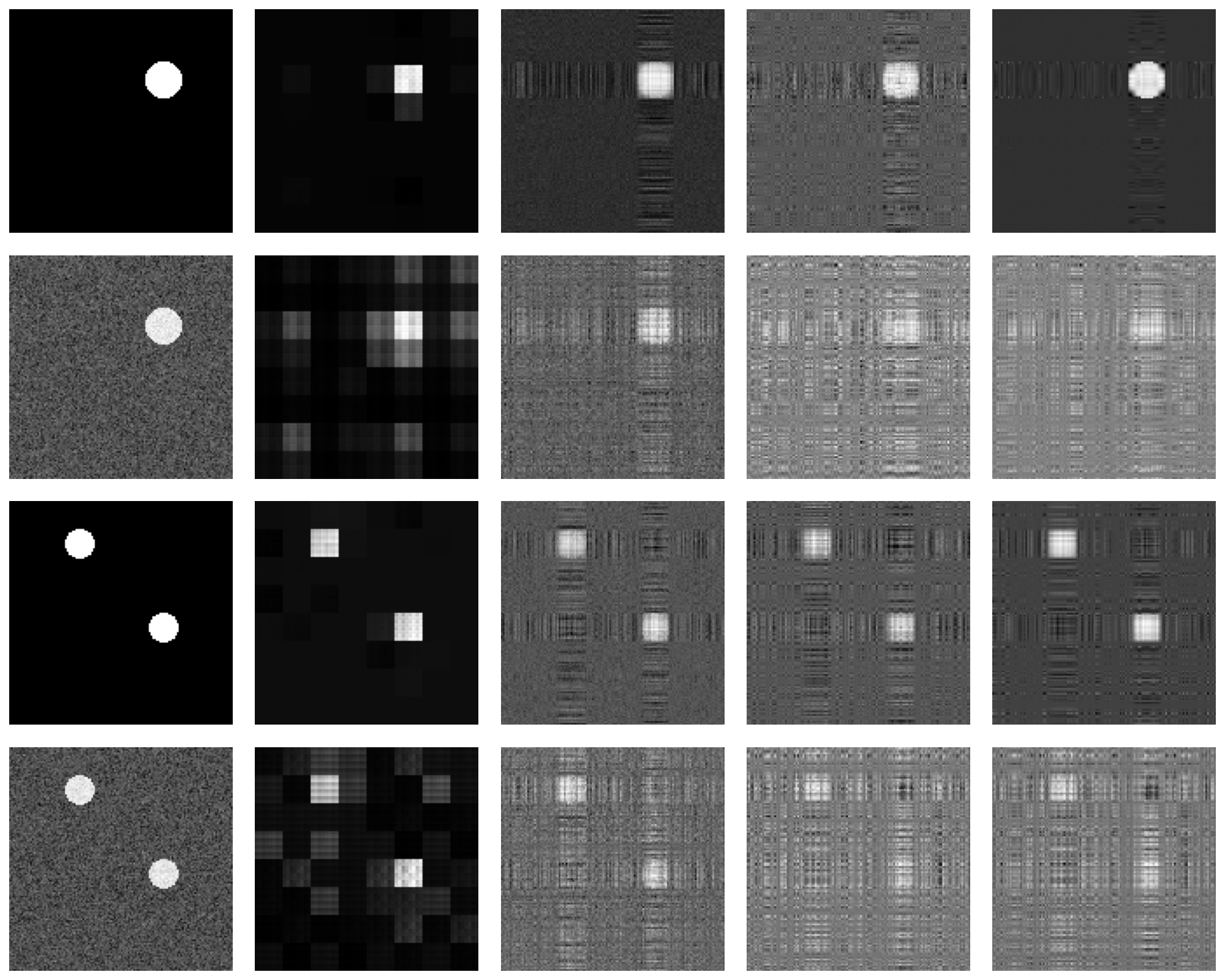
Figure 3: An illustration of the estimated coefficients $\boldsymbol{C}$ under $n=1000$. Rows from top to bottom: sparse one circle, quasi-sparse one circle, sparse two circles, quasi-sparse two circle. Columns from left to right: true signal, DKN, LRMR, TR, TRLasso.

8 The ADNI analysis

In this section, we use MRI data to analyze the Alzheimer’s Disease (AD), with data collected from the Alzheimer’s Disease Neuroimaging Initiative (ADNI). The ADNI is a study designed to detect and track Alzheimer’s disease with clinical, genetic, imaging data, etc. We refer to the website https://adni.loni.usc.edu/ for more details.

In the ADNI analysis, we use MRI data to analyze two types of outcomes: i) binary outcomes suggesting whether the participants have AD or not, and ii) continuous outcomes suggesting the Mini-Mental State Examination (MMSE) score of participants. The MMSE score is designed to assess the cognitive impairment of a patient. By Tombaugh and McIntyre, (1992), an MMSE score falling in the region of [24, 30], [19, 23], [10, 18] and [0, 9] suggests no, mild, moderate, and severe cognitive impairment, respectively. Therefore, the MMSE score could also be viewed as a reference for the diagnosis of Alzheimer’s disease. In other word, the two outcomes considered here are highly correlated.

The ADNI has four phases of study until today: ADNI-1, ADNI-GO, ADNI-2 and ADNI-3. As ADNI-3 is still ongoing, our analysis focuses on the first three phases. Specifically, we use data in ADNI-1 and ADNI-GO phase as training set while data in ADNI-2 phase as test set. The training set and test set contains 417 and 241 subjects, respectively. We provide distributions of binary outcome AD and MMSE in the supplementary material.

Each participant in the analysis is involved with a T1-weighted MRI scan. The T1-weighted MRI scan were carefully preprocessed before analysis. A standard pipeline proceeds as follows: spatial adaptive non-local means (SANLM) denoising (Manjón et al.,, 2010), resampling, bias-correction, affine-registration and unified segmentation, skull-stripping and cerebellum removing Ashburner and Friston, (2005). It then followed by local intensity correction and spatial normalization (into the Montreal Neurological Institute (MNI) atlas space). To this end, each T1-weighted MRI scan is processed into a tensor of size $113\times 137\times 113$. To improve analytical efficiency, we first resize each image into a smaller tensor and conduct zero-padding. The finally obtained images are represented as tensors of size $64\times 64\times 64$.

8.1 Regression analysis for MMSE

In this subsection, we use the MRI data to predict the MMSE score. As discussed before, the MMSE score is a continuous outcome ranging from 0 to 30. Normal people usually has an MMSE score close to 30 (mean 28.82, s.d. 1.02 in our dataset). While for AD patients, the mean and standard deviation are 21.63 and 3.25, respectively.

As in the simulation study, we implement the DKN under the deepest possible model. Specifically, we consider a 6-layer DKN with factors $\mathbf{\mathcal{B}}_{l}^{r}$ of size $(2\times 2\times 2)$. We still consider DKN models with the rank selected by BIC. Moreover, the performance of DKN is compared with TR, TRLasso and CNN. Note that we are not implementing the LRMR as it is unable to be generalized for tensor inputs. For CNN, we employ a network with structure similar to that in Hu et al., (2020), who also studied MRI data using CNN. Specifically, we consider a network with two convolutional layers, two max-poolings, and 2 fully connected layers. In the convolutional layer, the kernel is of size $3\times 3\times 3$ and stride is $1\times 1\times 1$. In the max-pooling layer, the kernel is of size $2\times 2\times 2$. We use ReLU activation and apply the batch normalization.

Task	Criterion	DKN	TR	TRLasso	CNN
Regression	RMSE	0.2258	0.2627	0.2557	0.2909
Classification	Accuracy	79.25%	66.80%	76.76%	78.01%

Table 2: The performance of algorithms on regression and classification tasks. In each task, the best result is marked as green.

We report the test set (ADNI-2) prediction accuracy of different methods in Table 2. In addition, for DKN and two TR approaches, we also plot the estimated coefficients in Fig 4 (left). Note that the tensor coefficients of DKN and TR are plotted after thresholding to better illustrate the detected regions.

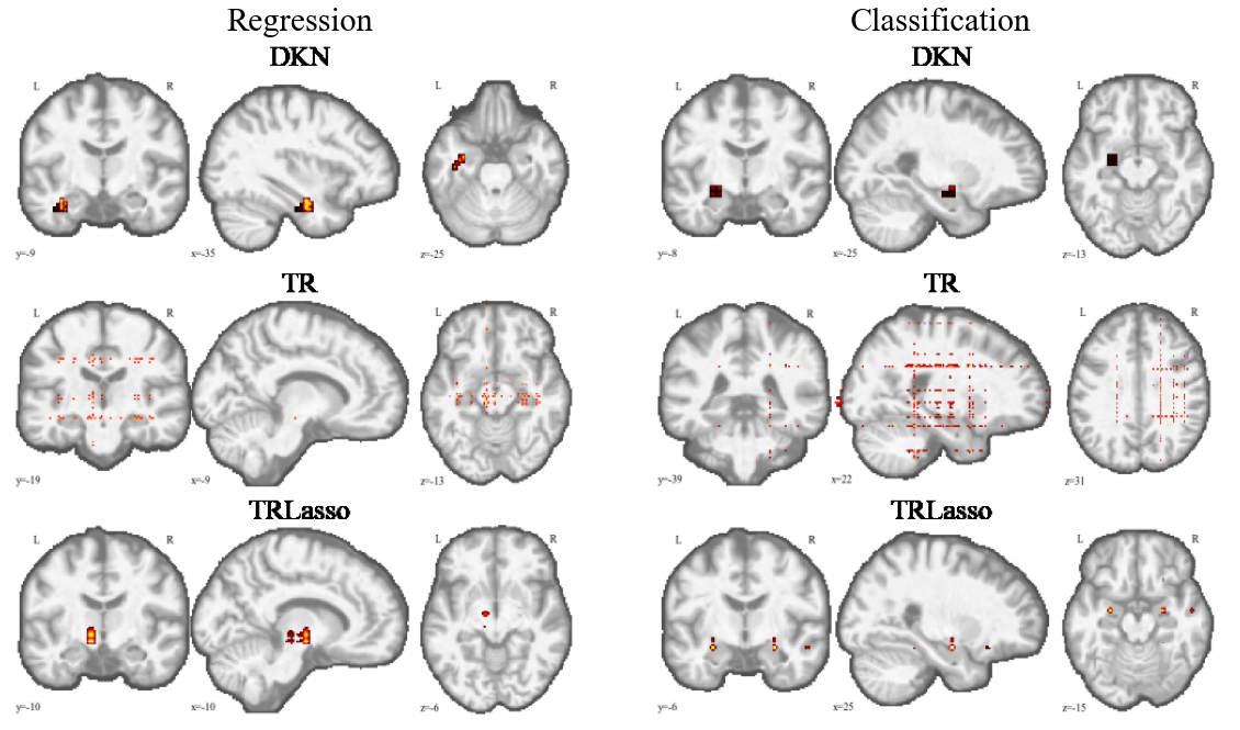
Figure 4: The detected brain regions in MMSE regression and AD classification.

By Table 2, DKN clearly performs the best with smallest prediction error. As a comparison, the CNN obtains the largest RMSE, suggesting a larger sample size is needed for CNN. Moreover, by Figure 4, the brain region detected by DKN are indicating an area around the hippocampus, which has been shown in medical literature is associated with AD (to be discussed in detail later). While for TR and TRLasso, they failed to capture the region of hippocampus, resulting to compromised prediction accuracy.

In the literature, the hippocampus has been proved to be associated with Alzheimer’s disease. For example, the early work of Ball et al., (1985) has attributed the decline of higher cognitive functions in AD to the hippocampus and proposed to name AD as a hippocampal dementia. Dubois et al., (2016) revealed that AD would gradually destroy different areas of brain cells and hippocampus is one of the regions suffering the damage first. Therefore, we are able to claim that the findings of DKN is in line with existing medical literature.

8.2 Classification analysis for AD

In this subsection, we conduct a binary classification analysis that uses MRI data to predict the participants’ AD status. The training set contains 417 subjects with $45\%$ AD patients, while the test set contains 241 subjects with $42\%$ AD patients.

We employ the same DKN structure as in the regression analysis: the number of layers $L=6$, the factors $\mathbf{\mathcal{B}}_{l}^{r}$ are of size $(2\times 2\times 2)$ and Kronecker ranks tuned by BIC. For DKN, TR and TRLasso, a logit link function is employed for such a binary classification task. While for CNN, we also use the same structure described in the regression analysis (two convolutional layer, two max-pooling and two fully connected layers), but with a soft-max output function for the classification problem.

The classification accuracy and region detection results are reported in Table 2 and Fig 4 (right), respectively. We again observe that DKN achieved the highest classification accuracy. On the other hand, we note that although TRLasso performs a little worse, the TR without regularization performs the worst among all methods. In terms of region detection performance, we see that the brain areas detected by DKN and TRLasso are all located around hippocampus, but the TR again failed to capture such area.

Combining the regression and classification analyses, we see that DKN is the only approach that is able to locate hippocampus under both analyses. In conclusion, the DKN could not only achieve the best possible prediction accuracy under limited sample size, more importantly, it could also provide desired interpretability and help medical researchers understanding imaging data better.

Supplementary material

In the supplementary material, we provide proofs of Theorem 6.4 to Theorem 6.7 along with additional details for the ADNI analysis. We omit the proofs of Theorem 4.1 to Theorem 6.1 and Proposition 1 as they could either be derived easily by algebra or follow directly from Lemmas discussed earlier. We provide proofs in the order of Theorem 6.6, Theorem 6.4 and Theorem 6.7. To get started, we first need some additional lemmas (Lemma S1.1 to Lemma S1.7).

S1 Proofs

Lemma S1.1.

For any two vectors $\boldsymbol{u},\boldsymbol{v}\in\mathbb{R}^{d}$, we have:

$$\text{dist}^{2}(\boldsymbol{u},\boldsymbol{v}) \leq \left(\frac{\boldsymbol{u}}{\|\boldsymbol{u}\|_{2}}-\frac{\boldsymbol{v}}{\|\boldsymbol{v}\|_{2}}\right)^{2}$$

$$\text{dist}^{2}(\boldsymbol{u},\boldsymbol{v}) \leq \frac{\|\boldsymbol{u}-\boldsymbol{v}\|_{2}^{2}}{\|\boldsymbol{u}\|_{2}^{2}}$$

$$\text{dist}^{2}(\boldsymbol{u},\boldsymbol{v}) \leq \frac{\|\boldsymbol{u}-\boldsymbol{v}\|_{2}^{2}}{\|\boldsymbol{v}\|_{2}^{2}}$$

Moreover, for any vectors $\boldsymbol{u},{\widehat{\boldsymbol{u}}},\boldsymbol{v},{\widehat{\boldsymbol{v}}}\in\mathbb{R}^{d}$,

$$\text{dist}^{2}(\boldsymbol{u}\boldsymbol{v}^{\top},\ {\widehat{\boldsymbol{u}}}{\widehat{\boldsymbol{v}}}^{\top}) = \text{dist}^{2}(\boldsymbol{u},{\widehat{\boldsymbol{u}}})^{2}+\text{dist}^{2}(\boldsymbol{v},{\widehat{\boldsymbol{v}}})-\text{dist}^{2}(\boldsymbol{u},{\widehat{\boldsymbol{u}}})\text{dist}^{2}(\boldsymbol{v},{\widehat{\boldsymbol{v}}})$$

It further follows that

$$\text{dist}^{2}(\boldsymbol{u}\boldsymbol{v}^{\top},\ {\widehat{\boldsymbol{u}}}{\widehat{\boldsymbol{v}}}^{\top}) \leq \text{dist}^{2}(\boldsymbol{u},{\widehat{\boldsymbol{u}}})+\text{dist}^{2}(\boldsymbol{v},{\widehat{\boldsymbol{v}}})$$

$$\text{dist}(\boldsymbol{u}\boldsymbol{v}^{\top},\ {\widehat{\boldsymbol{u}}}{\widehat{\boldsymbol{v}}}^{\top}) \leq \text{dist}(\boldsymbol{u},{\widehat{\boldsymbol{u}}})+\text{dist}(\boldsymbol{v},{\widehat{\boldsymbol{v}}})$$

$$\text{dist}(\boldsymbol{u}\boldsymbol{v}^{\top},\ {\widehat{\boldsymbol{u}}}{\widehat{\boldsymbol{v}}}^{\top}) \geq \text{dist}(\boldsymbol{u},{\widehat{\boldsymbol{u}}})\text{dist}(\boldsymbol{v},{\widehat{\boldsymbol{v}}})$$

Furthermore, for any matrices $\boldsymbol{U},{\widehat{\boldsymbol{U}}}\in\mathbb{R}^{d_{1}\times p_{1}}$ and $\boldsymbol{V},{\widehat{\boldsymbol{V}}}\in\mathbb{R}^{d_{2}\times p_{2}}$

$$\text{max}\left\{\text{dist}(\boldsymbol{U},{\widehat{\boldsymbol{U}}}),\ \text{dist}(\boldsymbol{V},{\widehat{\boldsymbol{V}}})\right\}\leq\text{dist}(\boldsymbol{U}\otimes\boldsymbol{V},{\widehat{\boldsymbol{U}}}\otimes{\widehat{\boldsymbol{V}}})\leq\text{dist}(\boldsymbol{U},{\widehat{\boldsymbol{U}}})+\text{dist}(\boldsymbol{V},{\widehat{\boldsymbol{V}}}).$$

More generally, for any matrices $\boldsymbol{U}_{k},\ {\widehat{\boldsymbol{U}}}_{k}\in\mathbb{R}^{d_{k}\times p_{k}}$, $k=1,2\ldots,l$, denote $\boldsymbol{U}_{(:)}=\bigotimes_{k=1}^{l}\boldsymbol{U}_{k}$ and ${\widehat{\boldsymbol{U}}}_{(:)}=\bigotimes_{k=1}^{l}{\widehat{\boldsymbol{U}}}_{k}$, we have

$$\max_{k=1,\ldots,l}\left\{\text{dist}\left(\boldsymbol{U}_{k},{\widehat{\boldsymbol{U}}}_{k}\right)\right\}\leq\text{dist}\left(\boldsymbol{U}_{(:)},{\widehat{\boldsymbol{U}}}_{(:)}\right)\leq\sum_{k=1}^{l}\text{dist}\left(\boldsymbol{U}_{k},{\widehat{\boldsymbol{U}}}_{k}\right).$$

We omit the proof of Lemma S1.1 as it could be derived easily by algebra. $\square$

Lemma S1.2.

Suppose the Condition 1 holds for ${\bf{\mathcal{X}}}_{i}$. Then for any $\mathbf{\mathcal{B}}_{l}^{r}$, $l=1,\ldots,L$, $r=1,2$, we have

$$\left|\frac{1}{n}\sum_{i=1}^{n}\left\langle{\bf{\mathcal{X}}}_{i},\bigotimes_{l=L}^{1}\mathbf{\mathcal{B}}_{l}^{1}\right\rangle\left\langle{\bf{\mathcal{X}}}_{i},\bigotimes_{l=L}^{1}\mathbf{\mathcal{B}}_{l}^{2}\right\rangle-\left\langle\bigotimes_{l=L}^{1}\mathbf{\mathcal{B}}_{l}^{1},\bigotimes_{l=L}^{1}\mathbf{\mathcal{B}}_{l}^{2}\right\rangle\right|\leq 3\delta\left\|\bigotimes_{l=L}^{1}\mathbf{\mathcal{B}}_{l}^{1}\right\|_{F}\left\|\bigotimes_{l=L}^{1}\mathbf{\mathcal{B}}_{l}^{2}\right\|_{F}$$

Proof of Lemma S1.2. Due to Condition 1,

$$\frac{1}{n}\sum_{i=1}^{n}\left\langle{\bf{\mathcal{X}}}_{i},\ \ \sum_{r=1}^{2}\bigotimes_{l=L}^{1}\mathbf{\mathcal{B}}_{l}^{r}\right\rangle^{2}\leq(1+\delta)\left\|\sum_{r=1}^{2}\bigotimes_{l=L}^{1}\mathbf{\mathcal{B}}_{l}^{r}\right\|^{2}_{F}$$

$$\Rightarrow \frac{1}{n}\sum_{i=1}^{n}\left\langle{\bf{\mathcal{X}}}_{i},\bigotimes_{l=L}^{1}\mathbf{\mathcal{B}}_{l}^{1}\right\rangle^{2}+\frac{1}{n}\sum_{i=1}^{n}\left\langle{\bf{\mathcal{X}}}_{i},\bigotimes_{l=L}^{1}\mathbf{\mathcal{B}}_{l}^{2}\right\rangle^{2}+\frac{2}{n}\sum_{i=1}^{n}\left\langle{\bf{\mathcal{X}}}_{i},\bigotimes_{l=L}^{1}\mathbf{\mathcal{B}}_{l}^{1}\right\rangle\left\langle{\bf{\mathcal{X}}}_{i},\bigotimes_{l=L}^{1}\mathbf{\mathcal{B}}_{l}^{2}\right\rangle$$

$$\leq(1+\delta)\left(\left\|\bigotimes_{l=L}^{1}\mathbf{\mathcal{B}}_{l}^{1}\right\|^{2}_{F}+\left\|\bigotimes_{l=L}^{1}\mathbf{\mathcal{B}}_{l}^{2}\right\|^{2}_{F}\right)+2(1+\delta)\left\langle\bigotimes_{l=L}^{1}\mathbf{\mathcal{B}}_{l}^{1},\bigotimes_{l=L}^{1}\mathbf{\mathcal{B}}_{l}^{2}\right\rangle$$

$$\Rightarrow \frac{1}{n}\sum_{i=1}^{n}\left\langle{\bf{\mathcal{X}}}_{i},\bigotimes_{l=L}^{1}\mathbf{\mathcal{B}}_{l}^{1}\right\rangle\left\langle{\bf{\mathcal{X}}}_{i},\bigotimes_{l=L}^{1}\mathbf{\mathcal{B}}_{l}^{2}\right\rangle-\left\langle\bigotimes_{l=L}^{1}\mathbf{\mathcal{B}}_{l}^{1},\bigotimes_{l=L}^{1}\mathbf{\mathcal{B}}_{l}^{2}\right\rangle$$

$$\leq\delta\left(\left\|\bigotimes_{l=L}^{1}\mathbf{\mathcal{B}}_{l}^{1}\right\|^{2}_{F}+\left\|\bigotimes_{l=L}^{1}\mathbf{\mathcal{B}}_{l}^{2}\right\|^{2}_{F}\right)+\delta\left\langle\bigotimes_{l=L}^{1}\mathbf{\mathcal{B}}_{l}^{1},\bigotimes_{l=L}^{1}\mathbf{\mathcal{B}}_{l}^{2}\right\rangle$$

$$\Rightarrow \frac{1}{n}\sum_{i=1}^{n}\left\langle{\bf{\mathcal{X}}}_{i},\bigotimes_{l=L}^{1}\mathbf{\mathcal{B}}_{l}^{1}\right\rangle\left\langle{\bf{\mathcal{X}}}_{i},\bigotimes_{l=L}^{1}\mathbf{\mathcal{B}}_{l}^{2}\right\rangle-\left\langle\bigotimes_{l=L}^{1}\mathbf{\mathcal{B}}_{l}^{1},\bigotimes_{l=L}^{1}\mathbf{\mathcal{B}}_{l}^{2}\right\rangle$$

$$\leq\delta\left(\left\|\bigotimes_{l=L}^{1}\mathbf{\mathcal{B}}_{l}^{1}\right\|^{2}_{F}+\left\|\bigotimes_{l=L}^{1}\mathbf{\mathcal{B}}_{l}^{2}\right\|^{2}_{F}\right)+\delta\left\|\bigotimes_{l=L}^{1}\mathbf{\mathcal{B}}_{l}^{1}\right\|_{F}\left\|\bigotimes_{l=L}^{1}\mathbf{\mathcal{B}}_{l}^{2}\right\|_{F}$$

where the third inequality holds due to the LHS of (25). Furthermore, we note that the last inequality still holds if we replace $\bigotimes_{l=L}^{1}\mathbf{\mathcal{B}}_{l}^{1}$ by $\lambda\bigotimes_{l=L}^{1}\mathbf{\mathcal{B}}_{l}^{1}$ and replace $\bigotimes_{l=L}^{1}\mathbf{\mathcal{B}}_{l}^{2}$ by $(1/\lambda)\bigotimes_{l=L}^{1}\mathbf{\mathcal{B}}_{l}^{2}$. Optimizing the RHS with $\lambda$, we get

$$\frac{1}{n}\sum_{i=1}^{n}\left\langle{\bf{\mathcal{X}}}_{i},\bigotimes_{l=L}^{1}\mathbf{\mathcal{B}}_{l}^{1}\right\rangle\left\langle{\bf{\mathcal{X}}}_{i},\bigotimes_{l=L}^{1}\mathbf{\mathcal{B}}_{l}^{2}\right\rangle-\left\langle\bigotimes_{l=L}^{1}\mathbf{\mathcal{B}}_{l}^{1},\bigotimes_{l=L}^{1}\mathbf{\mathcal{B}}_{l}^{2}\right\rangle\leq 3\delta\left\|\bigotimes_{l=L}^{1}\mathbf{\mathcal{B}}_{l}^{1}\right\|_{F}\left\|\bigotimes_{l=L}^{1}\mathbf{\mathcal{B}}_{l}^{2}\right\|_{F}.$$

The other side of the inequality could be proved similarly. This completes the proof. $\square$

Lemma S1.3.

Suppose that $\|\mathbf{\mathcal{B}}_{l}\|=1$ and $\|\widehat{\mathbf{\mathcal{B}}}_{l}\|=1$, $l=l,\ldots,L$. Define ${\widehat{\boldsymbol{\Sigma}}}_{(l)}^{(t)}$ and $\boldsymbol{\Sigma}_{(l)}^{(t)}$ respectively as

$${\widehat{\boldsymbol{\Sigma}}}_{(l)}^{(t)}=(1/n)\sum_{i=1}^{n}\left[\widehat{\boldsymbol{Z}}_{i}^{(l)}\right]^{(t)}{\widehat{\boldsymbol{b}}}_{(l-1:)}^{(t+1)}\left[{\widehat{\boldsymbol{b}}}_{(l-1:)}^{(t+1)}\right]^{\top}\left(\left[\widehat{\boldsymbol{Z}}_{i}^{(l)}\right]^{(t)}\right)^{\top}$$

$$\boldsymbol{\Sigma}_{(l)}^{(t)}=(1/n)\sum_{i=1}^{n}\left[\widehat{\boldsymbol{Z}}_{i}^{(l)}\right]^{(t)}{\widehat{\boldsymbol{b}}}_{(l-1:)}^{(t+1)}\left[{\widehat{\boldsymbol{b}}}_{(l-1:)}^{(t+1)}\right]^{\top}\left(\boldsymbol{Z}_{i}^{(l)}\right)^{\top}.$$

Then we have

$$\left\|\left({\widehat{\boldsymbol{\Sigma}}}_{(l)}^{(t)}\right)^{-1}\left(\langle{\widehat{\boldsymbol{b}}}^{(t)}_{:l+1},\boldsymbol{b}_{:l+1}\rangle{\widehat{\boldsymbol{\Sigma}}}_{(l)}^{(t)}-\boldsymbol{\Sigma}_{(l)}^{(t)}\right)\right\|_{2}\leq\frac{3\delta}{1-3\delta}\text{dist}\left({\widehat{\boldsymbol{b}}}_{(:l+1)}^{(t)},\boldsymbol{b}_{(:l+1)}\right).$$

Proof of Lemma S1.3. The minimum eigenvalue of ${\widehat{\boldsymbol{\Sigma}}}_{(l)}^{(t)}$ is given by

$$\lambda_{\min}\left({\widehat{\boldsymbol{\Sigma}}}_{(l)}^{(t)}\right)$$ (S1)

$$= \min_{\|\boldsymbol{b}_{l}\|_{2}=1}\boldsymbol{b}_{l}^{\top}{\widehat{\boldsymbol{\Sigma}}}_{(l)}^{(t)}\boldsymbol{b}_{l}$$ (S2)

$$= (1/n)\sum_{i=1}^{n}\boldsymbol{b}_{l}^{\top}\left[\widehat{\boldsymbol{Z}}_{i}^{(l)}\right]^{(t)}{\widehat{\boldsymbol{b}}}_{(l-1:)}^{(t+1)}\left[{\widehat{\boldsymbol{b}}}_{(l-1:)}^{(t+1)}\right]^{\top}\left(\left[\widehat{\boldsymbol{Z}}_{i}^{(l)}\right]^{(t)}\right)^{\top}\boldsymbol{b}_{l}$$ (S3)

$$= (1/n)\min_{\|\boldsymbol{b}_{l}\|_{2}=1}\sum_{i=1}^{n}\text{tr}\left(\left[\widehat{\boldsymbol{Z}}_{i}^{(l)}\right]^{(t)}{\widehat{\boldsymbol{b}}}_{(l-1:)}^{(t+1)}\boldsymbol{b}_{l}^{\top}\right)\text{tr}\left(\left[\widehat{\boldsymbol{Z}}_{i}^{(l)}\right]^{(t)}{\widehat{\boldsymbol{b}}}_{(l-1:)}^{(t+1)}\boldsymbol{b}_{l}^{\top}\right)$$ (S4)

$$= (1/n)\sum_{i=1}^{n}\left\langle{\bf{\mathcal{X}}}_{i},\widehat{\mathbf{\mathcal{B}}}_{(:l+1)}\otimes\mathbf{\mathcal{B}}_{l}\otimes\widehat{\mathbf{\mathcal{B}}}_{(l-1:)}\right\rangle^{2}$$ (S5)

$$\geq 1-3\delta.$$ (S6)

where the last inequality holds by Lemma S1.2. Further consider the term

$$\left\|\langle{\widehat{\boldsymbol{b}}}_{(:l+1)}^{(t)},\boldsymbol{b}_{(:l+1)}\rangle{\widehat{\boldsymbol{\Sigma}}}_{(l)}^{(t)}-\boldsymbol{\Sigma}_{(l)}^{(t)}\right\|_{2}$$ (S7)

$$= \max_{\|\boldsymbol{u}\|_{2}=1,\|\boldsymbol{v}\|_{2}=1}\boldsymbol{u}^{\top}\left(\langle{\widehat{\boldsymbol{b}}}_{:l+1}^{(t)},\boldsymbol{b}_{:l+1}\rangle{\widehat{\boldsymbol{\Sigma}}}_{(l)}^{(t)}-\boldsymbol{\Sigma}_{(l)}^{(t)}\right)\boldsymbol{v}$$ (S8)

$$= \max_{\|\boldsymbol{u}\|_{2}=1,\|\boldsymbol{v}\|_{2}=1}\sum_{i=1}^{n}\Big{\{}\langle{\widehat{\boldsymbol{b}}}_{(:l+1)}^{(t)},\boldsymbol{b}_{(:l+1)}\rangle\boldsymbol{u}^{\top}\left[\widehat{\boldsymbol{Z}}^{(l)}_{i}\right]^{(t)}{\widehat{\boldsymbol{b}}}_{(l-1:)}{\widehat{\boldsymbol{b}}}_{(l-1:)}^{\top}\left(\left[\widehat{\boldsymbol{Z}}^{(l)}_{i}\right]^{(t)}\right)^{\top}\boldsymbol{v}$$ (S10)

$$\ \ \ \ \ \ \ \ \ \ \ \ \ \ \ \ \ \ \ \ \ \ -\boldsymbol{u}^{\top}\left[\widehat{\boldsymbol{Z}}^{(l)}_{i}\right]^{(t)}{\widehat{\boldsymbol{b}}}_{(l-1:)}{\widehat{\boldsymbol{b}}}_{(l-1:)}^{\top}\left(\boldsymbol{Z}^{(l)}_{i}\right)^{\top}\boldsymbol{v}\Big{\}}$$

$$= \max_{\|\boldsymbol{u}\|_{2}=1,\|\boldsymbol{v}\|_{2}=1}\sum_{i=1}^{n}\left\langle{\bf{\mathcal{X}}}_{i},\ \widehat{\mathbf{\mathcal{B}}}_{(:l+1)}\otimes\boldsymbol{U}\otimes\widehat{\mathbf{\mathcal{B}}}_{(l-1:)}\right\rangle$$ (S13)

$$\ \ \ \ \ \ \ \ \ \ \ \ \ \ \ \ \ \ \times\left\langle{\bf{\mathcal{X}}}_{i},\ \left(\langle{\widehat{\boldsymbol{b}}}_{(:l+1)}^{(t)},\boldsymbol{b}_{(:l+1)}\rangle\widehat{\mathbf{\mathcal{B}}}_{(:l+1)}\right)\otimes\boldsymbol{V}\otimes\widehat{\mathbf{\mathcal{B}}}_{(l-1:)}\right\rangle$$

$$\ \ \ \ \ \ \ \ \ \ \ \ \ \ \ \ \ \ -\left\langle{\bf{\mathcal{X}}}_{i},\ \widehat{\mathbf{\mathcal{B}}}_{(:l+1)}\otimes\boldsymbol{U}\otimes\widehat{\mathbf{\mathcal{B}}}_{(l-1:)}\right\rangle\left\langle{\bf{\mathcal{X}}}_{i},\ \mathbf{\mathcal{B}}_{(:l+1)}\otimes\boldsymbol{V}\otimes\widehat{\mathbf{\mathcal{B}}}_{(l-1:)}\right\rangle$$

$$= \max_{\|\boldsymbol{u}\|_{2}=1,\|\boldsymbol{v}\|_{2}=1}\sum_{i=1}^{n}\left\langle{\bf{\mathcal{X}}}_{i},\ \widehat{\mathbf{\mathcal{B}}}_{(:l+1)}\otimes\boldsymbol{U}\otimes\widehat{\mathbf{\mathcal{B}}}_{(l-1:)}\right\rangle$$ (S15)

$$\ \ \ \ \ \ \ \ \ \ \ \ \ \ \ \ \ \ \times\left\langle{\bf{\mathcal{X}}}_{i},\ \left(\langle{\widehat{\boldsymbol{b}}}_{(:l+1)}^{(t)},{\widehat{\boldsymbol{b}}}_{(:l+1)}\rangle\widehat{\mathbf{\mathcal{B}}}_{(:l+1)}-\mathbf{\mathcal{B}}_{(:l+1)}\right)\otimes\boldsymbol{V}\otimes\widehat{\mathbf{\mathcal{B}}}_{(l-1:)}\right\rangle$$

$$\leq 3\delta\sqrt{1-\left\langle{\widehat{\boldsymbol{b}}}_{(:l+1)}^{(t)},\boldsymbol{b}_{(:l+1)}\right\rangle^{2}}$$ (S16)

$$= 3\delta\ \text{dist}\left({\widehat{\boldsymbol{b}}}_{(:l+1)}^{(t)},\boldsymbol{b}_{(:l+1)}\right)$$ (S17)

The last inequality holds by Lemma S1.2. Combining (S1) and (S7), we have

$$\left\|\left({\widehat{\boldsymbol{\Sigma}}}_{(l)}^{(t)}\right)^{-1}\left(\langle{\widehat{\boldsymbol{b}}}^{(t)}_{:l+1},\boldsymbol{b}_{:l+1}\rangle{\widehat{\boldsymbol{\Sigma}}}_{(l)}^{(t)}-\boldsymbol{\Sigma}_{(l)}^{(t)}\right)\right\|_{2}\leq\frac{3\delta}{1-3\delta}\text{dist}\left({\widehat{\boldsymbol{b}}}_{(:l+1)}^{(t)},\boldsymbol{b}_{(:l+1)}\right).$$

$\square$

Lemma S1.4.

Suppose model (24) holds and Algorithm 1 is implemented under a correctly specified network structure. Let $\mu$ be the maximum of initial error, $\nu=\mu+3\delta/(1-3\delta)$ and $\kappa=(\nu+1)^{L}-(2\nu+1)$. If

$$\text{dist}\left({\widehat{\boldsymbol{b}}}_{(l-1:)}^{(t+1)},\boldsymbol{b}_{(l-1:)}\right)\leq\mu,\ \ \ \text{dist}\left({\widehat{\boldsymbol{b}}}_{(:l+1)}^{(t)},\boldsymbol{b}_{(:l+1)}\right)\leq\mu,$$

then

$$\text{dist}\left({\widehat{\boldsymbol{b}}}_{l}^{(t+1)},\boldsymbol{b}_{l}\right)\leq\nu\left(\text{dist}\left({\widehat{\boldsymbol{b}}}_{(l-1:)}^{(t+1)},\boldsymbol{b}_{(l-1:)}\right)+\text{dist}\left({\widehat{\boldsymbol{b}}}_{(:l+1)}^{(t)},\boldsymbol{b}_{(:l+1)}\right)\right)+\tau.$$ (S18)

Proof of Lemma S1.4. Lemma S1.4 provides the central inequality in our proof. For ease of presentation, we prove Lemma S1.4 for matrix images. The tensor case follows the same way. First recall that ${\widetilde{\boldsymbol{X}}}_{i}\left(\boldsymbol{b}_{(:l+1)},\boldsymbol{b}_{(l-1:)}\right)$ is defined as

$${\widetilde{\boldsymbol{X}}}_{i}\left(\boldsymbol{b}_{(:l+1)},\boldsymbol{b}_{(l-1:)}\right)=\mathcal{R}_{(d_{l},p_{l})}\left(\text{vec}^{-1}_{\left(d_{(l:)},p_{(l:)}\right)}\left(\boldsymbol{b}_{(:l+1)}^{\top}\mathcal{R}_{\left(d_{(:l+1)},p_{(:l+1)}\right)}(\boldsymbol{X}_{i})\right)\right)\boldsymbol{b}_{(l-1:)}.$$

Then we denote

$$\boldsymbol{Z}_{i}^{(l)}=\mathcal{R}_{(d_{l},p_{l})}\left(\text{vec}^{-1}_{\left(d_{(l:)},p_{(l:)}\right)}\left(\boldsymbol{b}_{(:l+1)}^{\top}\mathcal{R}_{\left(d_{(:l+1)},p_{(:l+1)}\right)}(\boldsymbol{X}_{i})\right)\right),$$

$$\left[\widehat{\boldsymbol{Z}}_{i}^{(l)}\right]^{(t)}=\mathcal{R}_{(d_{l},p_{l})}\left(\text{vec}^{-1}_{\left(d_{(l:)},p_{(l:)}\right)}\left(\left[{\widehat{\boldsymbol{b}}}_{(:l+1)}^{(t)}\right]^{\top}\mathcal{R}_{\left(d_{(:l+1)},p_{(:l+1)}\right)}(\boldsymbol{X}_{i})\right)\right).$$

Moreover, let

$${\widehat{\boldsymbol{\Sigma}}}_{(l)}^{(t)}=(1/n)\sum_{i=1}^{n}\left[\widehat{\boldsymbol{Z}}_{i}^{(l)}\right]^{(t)}{\widehat{\boldsymbol{b}}}_{(l-1:)}^{(t+1)}\left[{\widehat{\boldsymbol{b}}}_{(l-1:)}^{(t+1)}\right]^{\top}\left(\left[\widehat{\boldsymbol{Z}}_{i}^{(l)}\right]^{(t)}\right)^{\top}$$

$$\boldsymbol{\Sigma}_{(l)}^{(t)}=(1/n)\sum_{i=1}^{n}\left[\widehat{\boldsymbol{Z}}_{i}^{(l)}\right]^{(t)}{\widehat{\boldsymbol{b}}}_{(l-1:)}^{(t+1)}\left[{\widehat{\boldsymbol{b}}}_{(l-1:)}^{(t+1)}\right]^{\top}\left(\boldsymbol{Z}_{i}^{(l)}\right)^{\top}$$

$$\boldsymbol{\Theta}_{(l)}^{(t)}=(1/n)\sum_{i=1}^{n}\left[\widehat{\boldsymbol{Z}}_{i}^{(l)}\right]^{(t)}{\widehat{\boldsymbol{b}}}_{(l-1:)}^{(t+1)}\boldsymbol{b}_{(l-1:)}^{\top}\left(\boldsymbol{Z}_{i}^{(l)}\right)^{\top}$$

Without loss of generality, suppose ${\widehat{\boldsymbol{b}}}_{(l-1:)}^{(t+1)}$ and ${\widehat{\boldsymbol{b}}}_{(:l+1)}^{(t)}$ are normalized such that ${\widehat{\boldsymbol{b}}}_{(l-1:)}^{(t+1)}={\widehat{\boldsymbol{b}}}_{(:l+1)}^{(t)}=1$.

Denote $\lambda=\|\mathcal{C}\|_{F}$. Given ${\widehat{\boldsymbol{b}}}_{(l-1:)}^{(t+1)}$ and ${\widehat{\boldsymbol{b}}}_{(:l+1)}^{(t)}$, we need to estimate ${\widehat{\boldsymbol{b}}}_{l}^{(t+1)}$. Denote the (normalized) estimates as ${\widehat{\boldsymbol{b}}}_{l}^{(t+1)}$ and its estimated norm as $\widehat{\lambda}^{(t+1)}$. Then,

$$\widehat{\lambda}^{(t+1)}{\widehat{\boldsymbol{b}}}_{l}^{(t+1)}$$

$$= \left(\frac{1}{n}{\widehat{\boldsymbol{X}}}_{(l)}^{\top}{\widehat{\boldsymbol{X}}}_{(l)}\right)^{-1}\frac{1}{n}{\widehat{\boldsymbol{X}}}_{(l)}^{\top}\left(\boldsymbol{X}_{(l)}\lambda\boldsymbol{b}_{l}+\boldsymbol{\varepsilon}\right)$$

$$= \left({\widehat{\boldsymbol{\Sigma}}}_{(l)}^{(t)}\right)^{-1}\left(\boldsymbol{\Theta}_{(l)}^{(t)}\lambda\boldsymbol{b}_{l}+\frac{1}{n}{\widehat{\boldsymbol{X}}}_{(l)}^{\top}\boldsymbol{\varepsilon}\right)$$

$$= \langle{\widehat{\boldsymbol{b}}}^{(t+1)}_{(l-1:)},\boldsymbol{b}_{(l-1:)}\rangle\lambda\boldsymbol{b}_{l}-\left({\widehat{\boldsymbol{\Sigma}}}_{(l)}^{(t)}\right)^{-1}\left(\langle{\widehat{\boldsymbol{b}}}^{(t+1)}_{(l-1:)},\boldsymbol{b}_{(l-1:)}\rangle{\widehat{\boldsymbol{\Sigma}}}_{(l)}^{(t)}-\boldsymbol{\Theta}_{(l)}^{(t)}\right)\lambda\boldsymbol{b}_{l}+\frac{1}{n}\left({\widehat{\boldsymbol{\Sigma}}}_{(l)}^{(t)}\right)^{-1}{\widehat{\boldsymbol{X}}}_{(l)}^{\top}\boldsymbol{\varepsilon}$$

$$= \langle{\widehat{\boldsymbol{b}}}^{(t+1)}_{(l-1:)},\boldsymbol{b}_{(l-1:)}\rangle\langle{\widehat{\boldsymbol{b}}}^{(t)}_{(:l+1)},\boldsymbol{b}_{(:l+1)}\rangle\lambda\boldsymbol{b}_{l}$$

$$-\left({\widehat{\boldsymbol{\Sigma}}}_{(l)}^{(t)}\right)^{-1}\left(\langle{\widehat{\boldsymbol{b}}}^{(t+1)}_{(l-1:)},\boldsymbol{b}_{(l-1:)}\rangle\left[\langle{\widehat{\boldsymbol{b}}}^{(t)}_{(:l+1)},\boldsymbol{b}_{(:l+1)}\rangle{\widehat{\boldsymbol{\Sigma}}}_{(l)}^{(t)}-\boldsymbol{\Sigma}_{(l)}^{(t)}\right]\right)\lambda\boldsymbol{b}_{l}$$

$$-\left({\widehat{\boldsymbol{\Sigma}}}_{(l)}^{(t)}\right)^{-1}\left(\langle{\widehat{\boldsymbol{b}}}^{(t+1)}_{(l-1:)},\boldsymbol{b}_{(l-1:)}\rangle\boldsymbol{\Sigma}_{(l)}^{(t)}-\boldsymbol{\Theta}_{(l)}^{(t)}\right)\lambda\boldsymbol{b}_{l}+\frac{1}{n}\left({\widehat{\boldsymbol{\Sigma}}}_{(l)}^{(t)}\right)^{-1}{\widehat{\boldsymbol{X}}}_{(l)}^{\top}\boldsymbol{\varepsilon},$$

where ${\widehat{\boldsymbol{X}}}_{(l)}$ and $\boldsymbol{X}_{(l)}$ are respectively

$${\widehat{\boldsymbol{X}}}_{(l)}=\left[{\widetilde{\boldsymbol{X}}}_{1}^{\top}\left({\widehat{\boldsymbol{b}}}_{(:l+1)}^{(t)},{\widehat{\boldsymbol{b}}}_{(l-1:)}^{(t+1)}\right),\cdots,{\widetilde{\boldsymbol{X}}}_{n}^{\top}\left({\widehat{\boldsymbol{b}}}_{(:l+1)}^{(t)},{\widehat{\boldsymbol{b}}}_{(l-1:)}^{(t+1)}\right)\right]^{\top},$$

$$\boldsymbol{X}_{(l)}=\left[{\widetilde{\boldsymbol{X}}}_{1}^{\top}\left(\boldsymbol{b}_{(:l+1)},\boldsymbol{b}_{(l-1:)}\right),\cdots,{\widetilde{\boldsymbol{X}}}_{n}^{\top}\left(\boldsymbol{b}_{(:l+1)},\boldsymbol{b}_{(l-1:)}\right)\right]^{\top}.$$

It then follows that

$$\frac{\|\widehat{\lambda}^{(t+1)}{\widehat{\boldsymbol{b}}}^{(t+1)}_{l}-\lambda\boldsymbol{b}_{l}\|_{2}}{\lambda}$$ (S19)

$$\leq \underbrace{\left|1-\langle{\widehat{\boldsymbol{b}}}^{(t+1)}_{(l-1:)},\boldsymbol{b}_{(l-1:)}\rangle\langle{\widehat{\boldsymbol{b}}}^{(t)}_{(:l+1)},\boldsymbol{b}_{(:l+1)}\rangle\right|^{1/2}}_{A1}$$ (S23)

$$+\underbrace{\left\|\left({\widehat{\boldsymbol{\Sigma}}}_{(l)}^{(t)}\right)^{-1}\left(\langle{\widehat{\boldsymbol{b}}}^{(t+1)}_{(l-1:)},\boldsymbol{b}_{(l-1:)}\rangle\left[\langle{\widehat{\boldsymbol{b}}}^{(t)}_{(:l+1)},\boldsymbol{b}_{(:l+1)}\rangle{\widehat{\boldsymbol{\Sigma}}}_{(l)}^{(t)}-\boldsymbol{\Sigma}_{(l)}^{(t)}\right]\right)\right\|_{2}}_{A2}$$

$$+\underbrace{\left\|\left({\widehat{\boldsymbol{\Sigma}}}_{(l)}^{(t)}\right)^{-1}\left(\langle{\widehat{\boldsymbol{b}}}^{(t+1)}_{(l-1:)},\boldsymbol{b}_{(l-1:)}\rangle\boldsymbol{\Sigma}_{(l)}^{(t)}-\boldsymbol{\Theta}_{(l)}^{(t)}\right)\right\|_{2}}_{A3}$$

$$+\underbrace{\frac{\left\|\left({\widehat{\boldsymbol{\Sigma}}}_{(l)}^{(t)}\right)^{-1}{\widehat{\boldsymbol{X}}}_{(l)}^{\top}\boldsymbol{E}\right\|_{2}}{\lambda}}_{\text{A4}}.$$

We will bound A1 to A4 separately. For A1, we have

$$\left|1-\langle{\widehat{\boldsymbol{b}}}^{(t+1)}_{(l-1:)},\boldsymbol{b}_{(l-1:)}\rangle\langle{\widehat{\boldsymbol{b}}}^{(t)}_{(:l+1)},\boldsymbol{b}_{(:l+1)}\rangle\right|$$

$$\leq \left|1-\langle{\widehat{\boldsymbol{b}}}^{(t+1)}_{(l-1:)},\boldsymbol{b}_{(l-1:)}\rangle^{2}\langle{\widehat{\boldsymbol{b}}}^{(t)}_{(:l+1)},\boldsymbol{b}_{(:l+1)}\rangle^{2}\right|$$

$$\leq \left|1-\langle{\widehat{\boldsymbol{b}}}^{(t+1)}_{(l-1:)},\boldsymbol{b}_{(l-1:)}\rangle^{2}\right|+\left|1-\langle{\widehat{\boldsymbol{b}}}^{(t)}_{(:l+1)},\boldsymbol{b}_{(:l+1)}\rangle^{2}\right|$$

$$= \text{dist}^{2}({\widehat{\boldsymbol{b}}}_{(l-1:)}^{(t+1)},\boldsymbol{b}_{(l-1:)})+\text{dist}^{2}({\widehat{\boldsymbol{b}}}_{(:l+1)}^{(t)},\boldsymbol{b}_{(:l+1)})$$

$$\leq \mu\text{dist}({\widehat{\boldsymbol{b}}}_{(l-1:)}^{(t+1)},\boldsymbol{b}_{(l-1:)})+\mu\text{dist}({\widehat{\boldsymbol{b}}}_{(:l+1)}^{(t)},\boldsymbol{b}_{(:l+1)})$$

The last inequality holds due to the condition $\text{dist}({\widehat{\boldsymbol{b}}}_{(l-1:)}^{(t+1)},\boldsymbol{b}_{(l-1:)})\leq\mu$ and $\text{dist}({\widehat{\boldsymbol{b}}}_{(:l+1)}^{(t)},\boldsymbol{b}_{(:l+1)})\leq\mu$. For the term A2, according to Lemma S1.3, we have

$$\left\|\left({\widehat{\boldsymbol{\Sigma}}}_{(l)}^{(t)}\right)^{-1}\left(\langle{\widehat{\boldsymbol{b}}}^{(t+1)}_{(l-1:)},\boldsymbol{b}_{(l-1:)}\rangle\left[\langle{\widehat{\boldsymbol{b}}}^{(t)}_{(:l+1)},\boldsymbol{b}_{(:l+1)}\rangle{\widehat{\boldsymbol{\Sigma}}}_{(l)}^{(t)}-\boldsymbol{\Sigma}_{(l)}^{(t)}\right]\right)\right\|_{2}$$

$$= \langle{\widehat{\boldsymbol{b}}}^{(t+1)}_{(l-1:)},\boldsymbol{b}_{(l-1:)}\rangle\left\|\left({\widehat{\boldsymbol{\Sigma}}}_{(l)}^{(t)}\right)^{-1}\left(\langle{\widehat{\boldsymbol{b}}}^{(t)}_{(:l+1)},\boldsymbol{b}_{(:l+1)}\rangle{\widehat{\boldsymbol{\Sigma}}}_{(l)}^{(t)}-\boldsymbol{\Sigma}_{(l)}^{(t)}\right)\right\|_{2}$$

$$\leq \frac{3\delta}{1-3\delta}\langle{\widehat{\boldsymbol{b}}}^{(t+1)}_{(l-1:)},\boldsymbol{b}_{(l-1:)}\rangle\ \text{dist}\left({\widehat{\boldsymbol{b}}}_{(:l+1)}^{(t)},\boldsymbol{b}_{(:l+1)}\right)$$

$$\leq \frac{3\delta}{1-3\delta}\text{dist}\left({\widehat{\boldsymbol{b}}}_{(:l+1)}^{(t)},\boldsymbol{b}_{(:l+1)}\right).$$

For the term A3, we similarly have

$$\left\|\left({\widehat{\boldsymbol{\Sigma}}}_{(l)}^{(t)}\right)^{-1}\left(\langle{\widehat{\boldsymbol{b}}}^{(t+1)}_{(l-1:)},{\widehat{\boldsymbol{b}}}_{(l-1:)}\rangle\boldsymbol{\Sigma}_{(l)}^{(t)}-\boldsymbol{\Theta}_{(l)}^{(t)}\right)\right\|_{2}\leq\frac{3\delta}{1-3\delta}\text{dist}\left({\widehat{\boldsymbol{b}}}_{(l-1:)}^{(t+1)},\boldsymbol{b}_{(l-1:)}\right).$$

For the term A4, we first note that $\left\|{\widehat{\boldsymbol{\Sigma}}}_{(l)}^{(t)}\right\|_{2}^{-1}\leq(1-3\delta)^{-1}$. Moreover,

$$\left\|\frac{1}{n}{\widehat{\boldsymbol{X}}}_{(l)}^{\top}\boldsymbol{\varepsilon}\right\|_{2}=\left\|\frac{1}{n}\sum_{i=1}^{n}\epsilon_{i}{\widetilde{\boldsymbol{X}}}_{i}\left({\widehat{\boldsymbol{b}}}_{(:l+1)}^{(t)},{\widehat{\boldsymbol{b}}}_{(l-1:)}^{(t+1)}\right)\right\|_{2}$$

$$\leq \sup\left\{\frac{1}{n^{2}}\left\|\sum_{i=1}^{n}\epsilon_{i}{\widetilde{\boldsymbol{X}}}_{i}\left(\boldsymbol{b}_{(:l+1)},\boldsymbol{b}_{(l-1:)}\right)\right\|_{2},\ \|\boldsymbol{b}_{(:l+1)}\|_{2}=\|\boldsymbol{b}_{(l-1:)}\|_{2}=1\right\}=\tau_{0}.$$

As a result, A4 could be bounded by

$$(1/\lambda)\left\|\left({\widehat{\boldsymbol{\Sigma}}}_{(l)}^{(t)}\right)^{-1}{\widehat{\boldsymbol{X}}}_{(l)}^{\top}\boldsymbol{E}\right\|_{2}\leq\frac{\tau_{0}}{\lambda(1-3\delta)}=\tau.$$

Combining A1 to A4, we have

$$(1/\lambda)\|\widehat{\lambda}^{(t+1)}{\widehat{\boldsymbol{b}}}^{(t+1)}_{l}-\lambda\boldsymbol{b}_{l}\|_{2}\leq\nu\ \left[\text{dist}({\widehat{\boldsymbol{b}}}_{(l-1:)}^{(t+1)},\boldsymbol{b}_{(l-1:)})+\text{dist}({\widehat{\boldsymbol{b}}}_{(:l+1)}^{(t)},\boldsymbol{b}_{(:l+1)})\right]+\tau,$$ (S24)

where we recall that $\nu=\mu+3\delta/(1-3\delta)$. On the other hand, due to Lemma S1.1,

$$\text{dist}({\widehat{\boldsymbol{b}}}_{l}^{(t+1)},\boldsymbol{b}_{l})=\text{dist}(\widehat{\lambda}^{(t+1)}{\widehat{\boldsymbol{b}}}_{l}^{(t+1)},\ \lambda\boldsymbol{b}_{l})\leq\frac{\|\widehat{\lambda}^{(t+1)}{\widehat{\boldsymbol{b}}}_{l}^{(t+1)}-\lambda\boldsymbol{b}_{l}\|_{2}}{\lambda}.$$ (S25)

It then follows from (S24) and (S25) that

$$\text{dist}({\widehat{\boldsymbol{b}}}_{l}^{(t+1)},\boldsymbol{b}_{l})\leq\nu\left(\text{dist}({\widehat{\boldsymbol{b}}}_{(l-1:)}^{(t+1)},\boldsymbol{b}_{(l-1:)})+\text{dist}({\widehat{\boldsymbol{b}}}_{(:l+1)}^{(t)},\boldsymbol{b}_{(:l+1)})\right)+\tau.$$ (S26)

This is the central inequality. Note that for the special case with $l=1$ and $l=L$, the central inequality reduces to

$$\text{dist}({\widehat{\boldsymbol{b}}}_{1}^{(t+1)},\boldsymbol{b}_{1}) \leq \nu\ \text{dist}({\widehat{\boldsymbol{b}}}_{(:2)}^{(t)},\boldsymbol{b}_{(:2)})+\tau,$$

$$\text{dist}({\widehat{\boldsymbol{b}}}_{L}^{(t+1)},\boldsymbol{b}_{L}) \leq \nu\ \text{dist}({\widehat{\boldsymbol{b}}}_{(L-1:)}^{(t+1)},\boldsymbol{b}_{(L-1:)})+\tau.$$

$\square$

Lemma S1.5.

For any given $t\geq 0$, assume $\text{dist}\left({\widehat{\boldsymbol{b}}}_{(:l)}^{(t)},\boldsymbol{b}_{(:l)}\right)\leq\mu$ holds for all $l=2,\cdots,L$. Let $\nu=\mu+3\delta/(1-3\delta)$, $\tau=(\tau_{0}/\|\mathcal{C}\|_{F})(1-3\delta)^{-1}$ and $\eta=\mu/(\mu+\tau/\nu)$. Suppose $\nu$ satisfies $(\nu+1)^{L-1}-1<\eta$. Suppose Condition 1 holds. Then, for all $l=1,2,\ldots,\ L$, we have

$$\text{dist}\left({\widehat{\boldsymbol{b}}}_{(l-1:)}^{(t+1)},\boldsymbol{b}_{(l-1:)}\right)\leq\mu$$

Proof of Lemma S1.5. We will prove a shaper inequality, Then Lemma S1.5 follows immediately. We will show that

$$\text{dist}\left({\widehat{\boldsymbol{b}}}_{(l-1:)}^{(t+1)},\boldsymbol{b}_{(l-1:)}\right)\leq\left[(\nu+1)^{l-1}-1\right]\mu+\frac{(\nu+1)^{l-1}-1}{\nu}\tau$$ (S27)

We prove by induction. When $l=1$, $\text{dist}\left({\widehat{\boldsymbol{b}}}_{(0:)}^{(t+1)},\boldsymbol{b}_{(0:)}\right)=0\leq 0$ holds immediately. Then suppose the statement holds for $l$, we prove it holds for $l+1$. First note that $\text{dist}\left({\widehat{\boldsymbol{b}}}_{(l-1:)}^{(t+1)},\boldsymbol{b}_{(l-1:)}\right)\leq\mu$ because

$$\text{dist}\left({\widehat{\boldsymbol{b}}}_{(l-1:)}^{(t+1)},\boldsymbol{b}_{(l-1:)}\right) \leq \left[(\nu+1)^{l-1}-1\right]\mu+\frac{(\nu+1)^{l-1}-1}{\nu}\tau$$

$$\leq \left[(\nu+1)^{L-1}-1\right]\left(\mu+\frac{\tau}{\nu}\right)$$

$$\leq \mu.$$

Combining the assumption $\text{dist}\left({\widehat{\boldsymbol{b}}}_{(:l+1)}^{(t)},\boldsymbol{b}_{(:l+1)}\right)\leq\mu$, we have inequality (S18) in Lemma S1.4 holds. Furthermore,

$$\text{dist}\left({\widehat{\boldsymbol{b}}}_{(l:)}^{(t+1)},\boldsymbol{b}_{(l:)}\right)$$

$$\leq \text{dist}\left({\widehat{\boldsymbol{b}}}_{l}^{(t+1)},\boldsymbol{b}_{l}\right)+\text{dist}\left({\widehat{\boldsymbol{b}}}_{(l-1:)}^{(t+1)},\boldsymbol{b}_{(l-1:)}\right)$$

$$\leq (\nu+1)\text{dist}\left({\widehat{\boldsymbol{b}}}_{(l-1:)}^{(t+1)},\boldsymbol{b}_{(l-1:)}\right)+\nu\text{dist}\left({\widehat{\boldsymbol{b}}}_{(:l+1)}^{(t)},\boldsymbol{b}_{(:l+1)}\right)+\tau$$

$$\leq (\nu+1)\left[(\nu+1)^{l-1}-1\right]\mu+(\nu+1)\frac{(\nu+1)^{l-1}-1}{\nu}\tau+\nu\mu+\tau$$

$$= \left[(\nu+1)^{l}-1\right]\mu+\frac{(\nu+1)^{l}-1}{\nu}\tau$$

These inequalities hold in turn by 1) Lemma S1.1, 2) inequality (S18) and 3) induction holds for $l$. Thus, the statement holds for $l+1$. As a consequence, we complete the proof of (S27). Finally, $\text{dist}\left({\widehat{\boldsymbol{b}}}_{(l-1:)}^{(t+1)},\boldsymbol{b}_{(l-1:)}\right)\leq\mu$ for all $l=1,\cdots,L$. $\square$

Lemma S1.6.

For any given $t\geq 0$, assume $\text{dist}\left({\widehat{\boldsymbol{b}}}_{(:l)}^{(t)},\boldsymbol{b}_{(:l)}\right)\leq\mu$ holds for all $l=2,\cdots,L$. Let $\nu=\mu+3\delta/(1-3\delta)$, $\tau=(\tau_{0}/\|\mathcal{C}\|_{F})(1-3\delta)^{-1}$ and $\eta=\mu/(\mu+\tau(\nu+1)/\nu)$. Suppose $\nu$ satisfies $(\nu+1)^{L-1}-1<\eta$. Suppose Condition 1 holds. Then

$$\text{dist}\left({\widehat{\boldsymbol{b}}}_{(:l)}^{(t+1)},\boldsymbol{b}_{(:l)}\right)\leq\mu$$

holds for all $l=2,\ldots,\ L$.

Proof of Lemma S1.6. Similar to Lemma S1.5, we prove the following shaper inequality holds by induction:

$$\text{dist}\left({\widehat{\boldsymbol{b}}}_{(:l)}^{(t+1)},\boldsymbol{b}_{(:l)}\right)\leq\left[(\nu+1)^{L-1}-(\nu+1)^{l-1}+\nu\right]\mu+\frac{(\nu+1)^{L}-(\nu+1)^{l-1}}{\nu}\tau.$$ (S28)

Before that, because conditions in Lemma S1.6 are also satisfied by Lemma S1.5, we have the inequality (S27) holds. Additionally, with the assumption $\text{dist}\left({\widehat{\boldsymbol{b}}}_{(:l)}^{(t)},\boldsymbol{b}_{(:l)}\right)\leq\mu$, Lemma S1.4 also holds.

For this induction, we start with $l=L$.

$$\text{dist}\left({\widehat{\boldsymbol{b}}}_{(:L)}^{(t+1)},\boldsymbol{b}_{(:L)}\right) = \text{dist}\left({\widehat{\boldsymbol{b}}}_{L}^{(t+1)},\boldsymbol{b}_{L}\right)$$

$$\leq \nu\text{dist}\left({\widehat{\boldsymbol{b}}}_{(L-1:)}^{(t+1)},\boldsymbol{b}_{(L-1:)}\right)+\tau$$

$$\leq \nu\left[(\nu+1)^{L-1}-1\right]\mu+\left[(\nu+1)^{L-1}-1\right]\tau+\tau$$

$$\leq \nu\mu+(\nu+1)^{L-1}\tau$$

These inequalities hold in turn by 1) Lemma S1.4 , 2) inequality (S27) and 3) $(\nu+1)^{L-1}-1<\eta<1$. Note that $\nu\mu=\left((\nu+1)^{L-1}-(\nu+1)^{L-1}+\nu\right)\mu$ and $(\nu+1)^{L-1}\tau=\left((\nu+1)^{L}-(\nu+1)^{L-1}\right)/\nu\cdot\tau$. Thus the statement holds for $l=L$.

Next we suppose the statement holds for $l$, to prove it holds for $l-1$.

$$\text{dist}\left({\widehat{\boldsymbol{b}}}_{(:l-1)}^{(t+1)},\boldsymbol{b}_{(:l-1)}\right)$$

$$\leq \text{dist}\left({\widehat{\boldsymbol{b}}}_{(:l)}^{(t+1)},\boldsymbol{b}_{(:l)}\right)+\text{dist}\left({\widehat{\boldsymbol{b}}}_{l-1}^{(t+1)},\boldsymbol{b}_{l-1}\right)$$

$$\leq \text{dist}\left({\widehat{\boldsymbol{b}}}_{(:l)}^{(t+1)},\boldsymbol{b}_{(:l)}\right)+\nu\left(\text{dist}\left({\widehat{\boldsymbol{b}}}_{(l-2:)}^{(t+1)},\boldsymbol{b}_{(l-2:)}\right)+\text{dist}\left({\widehat{\boldsymbol{b}}}_{(:l)}^{(t)},\boldsymbol{b}_{(:l)}\right)\right)+\tau$$

$$\leq \left[(\nu+1)^{L-1}-(\nu+1)^{l-1}+\nu\right]\mu+\frac{(\nu+1)^{L}-(\nu+1)^{l-1}}{\nu}\tau$$

$$+\nu\left\{\left[(\nu+1)^{l-2}-1\right]\mu+\frac{(\nu+1)^{l-2}-1}{\nu}\tau+\mu\right\}+\tau$$

$$= \left((\nu+1)^{L-1}-(\nu+1)^{l-2}+\nu\right)\mu+\frac{(\nu+1)^{L}-(\nu+1)^{l-2}}{\nu}\tau$$

These inequalities hold in turn by 1) Lemma S1.1, 2) lemma S1.4 and 3) induction in $l$ and inequality (S27). Thus, the inequality holds for $l-1$. So (S28) holds for all $l=2,\cdots,L$. Finally

$$\text{dist}\left({\widehat{\boldsymbol{b}}}_{(:l)}^{(t+1)},\boldsymbol{b}_{(:l)}\right)$$

$$\leq \left((\nu+1)^{L-1}-(\nu+1)^{l-1}+\nu\right)\mu+\frac{(\nu+1)^{L}-(\nu+1)^{l-1}}{\nu}\tau$$

$$= \left((\nu+1)^{L-1}-1\right)\left(\mu+\frac{\nu+1}{\nu}\tau\right)$$

$$\leq \mu$$

We complete the proof of Lemma S1.6. $\square$

Proof of Theorem 6.6

Now we are ready to prove Theorem 6.6. First, by Lemma S1.6, when $\text{dist}\left({\widehat{\boldsymbol{b}}}_{(:l)}^{(0)},\boldsymbol{b}_{(:l)}\right)\leq\mu$ for $l=2,\ldots,L$, we have $\text{dist}\left({\widehat{\boldsymbol{b}}}_{(:l)}^{(t)},\boldsymbol{b}_{(:l)}\right)\leq\mu$ holds for all $t=0,1,\ldots$ and $l=2,\ldots,L$ by a simple induction.

Next, when $\text{dist}\left({\widehat{\boldsymbol{b}}}_{(:l)}^{(t)},\boldsymbol{b}_{(:l)}\right)\leq\mu$ holds for all $t=0,1,\ldots$ and $l=2,\ldots,L$, by Lemma S1.5, we have $\text{dist}\left({\widehat{\boldsymbol{b}}}_{(l-1:)}^{(t+1)},\boldsymbol{b}_{(l-1:)}\right)\leq\mu$ holds for all $t=0,1,\ldots$ and $l=2,\ldots,L$.

Finally when $\text{dist}\left({\widehat{\boldsymbol{b}}}_{(:l)}^{(t)},\boldsymbol{b}_{(:l)}\right)\leq\mu$ and $\text{dist}\left({\widehat{\boldsymbol{b}}}_{(l-1:)}^{(t+1)},\boldsymbol{b}_{(l-1:)}\right)\leq\mu$ holds for all $t=0,1,\ldots$ and $l=2,\ldots,L$, we have Theorem 6.6 holds by Lemma S1.4. $\square$

Lemma S1.7.

Suppose model (24) holds and the RIP condition. Assume the noise $\epsilon_{i}$ is sub-Gaussian. Let

$$\tau_{0}=\sup\left\{\frac{1}{n}\Big{\|}\sum_{i=1}^{n}\epsilon_{i}{\widetilde{\boldsymbol{X}}}_{i}\left(\boldsymbol{b}_{(:l+1)},\ \boldsymbol{b}_{(l-1:)}\right)\Big{\|}_{2},\ \|\boldsymbol{b}_{(:l+1)}\|_{2}=\|\boldsymbol{b}_{(l-1:)}\|_{2}=1,\ l=1,\ldots,L\right\}.$$

and $\tau=(\tau_{0}/\|\mathcal{C}\|_{F})(1-3\delta)^{-1}$. Then,

$$\tau=\mathcal{O}_{p}\left(\sqrt{\frac{\log(n)}{n}}\right).$$

Proof of Lemma S1.7. By a Hoeffding-type inequality, e.g., Proposition 5.10 in Vershynin, (2010), we have

$${\mathbb{P}}\left\{\frac{1}{n^{2}}\left\|\sum_{i=1}^{n}\epsilon_{i}{\widetilde{\boldsymbol{X}}}_{i}\left(\boldsymbol{b}_{(:l+1)},\boldsymbol{b}_{(l-1:)}\right)\right\|_{2}^{2}\geq c_{0}\frac{\log n}{n}\left(\frac{1}{n}\sum_{i=1}^{n}\left\|{\widetilde{\boldsymbol{X}}}_{i}\left(\boldsymbol{b}_{(:l+1)},\boldsymbol{b}_{(l-1:)}\right)\right\|_{2}^{2}\right)\right\}\leq\frac{1}{n}$$

holds for certain constant $c_{0}$. Note that we may take sup on both side of inequality inside ${\mathbb{P}}\{\}$. On the other hand, for any ${\widetilde{\boldsymbol{X}}}_{i}$, $(1/n)\sum_{i=1}^{n}\left\|{\widetilde{\boldsymbol{X}}}_{i}\left(\boldsymbol{b}_{(:l+1)},\boldsymbol{b}_{(l-1:)}\right)\right\|_{2}^{2}$ is upper bounded due to the Condition 1. Therefore

$$\tau_{0}=\left\|{\widehat{\boldsymbol{X}}}_{(l)}^{\top}\boldsymbol{E}\right\|_{2}\leq c\sqrt{\frac{\log n}{n}}$$

holds with large probability, where $c$ is certain constant. Further we have the same order probabilistic upper bound for $\tau$. $\square$

Proof of Theorem 6.4

According to Theorem 6.6, inequality (27) holds for $t=0,1,\ldots$ and $l=1,\ldots,L$.

$$\text{dist}\left({\widehat{\boldsymbol{b}}}_{l}^{(t+1)},\boldsymbol{b}_{l}\right) \leq \nu\left(\text{dist}\left({\widehat{\boldsymbol{b}}}_{(l-1:)}^{(t+1)},\boldsymbol{b}_{(l-1:)}\right)+\text{dist}\left({\widehat{\boldsymbol{b}}}_{(:l+1)}^{(t)},\boldsymbol{b}_{(:l+1)}\right)\right)+\tau$$ (S29)

$$\leq \nu\sum_{j=1}^{l-1}\text{dist}\left({\widehat{\boldsymbol{b}}}_{j}^{(t+1)},\boldsymbol{b}_{j}\right)+\nu\sum_{j=l+1}^{L}\text{dist}\left({\widehat{\boldsymbol{b}}}_{j}^{(t)},\boldsymbol{b}_{j}\right)+\tau$$ (S30)

The second inequality holds by Lemma S1.1. Now we show that the following inequality follows from (S30):

$$\text{dist}\left({\widehat{\boldsymbol{b}}}_{l}^{(t+1)},\boldsymbol{b}_{l}\right)\leq\sum_{j=1}^{L}f(l,j)\text{dist}\left({\widehat{\boldsymbol{b}}}_{j}^{(t)},\boldsymbol{b}_{j}\right)+h(l)\tau$$ (S31)

where $f(l,j)$ and $h(l)$ are the coefficients function with the following form

$$f(l,j)=\nu\left((\nu+1)^{l-1}-I[l\geq j](\nu+1)^{l-j}\right)\quad\text{for}\ l,\ j=1,\cdots,L$$ (S32)

$$h(l)=(\nu+1)^{l-1}\quad\text{for}\ l=1,\cdots,L$$ (S33)

Again we prove (S31) by induction. For $l=1$,

$$\text{dist}\left({\widehat{\boldsymbol{b}}}_{1}^{(t+1)},\boldsymbol{b}_{1}\right) \leq \nu\text{dist}\left({\widehat{\boldsymbol{b}}}_{(:2)}^{(t)},\boldsymbol{b}_{(:2)}\right)+\tau\leq\sum_{j=2}^{L}\nu\text{dist}\left({\widehat{\boldsymbol{b}}}_{j}^{(t)},\boldsymbol{b}_{j}\right)+\tau$$

which indicates that $f(1,1)=0$ and $f(1,j)=\nu$ for $j=2,\cdots,L$, satisfying formulation (S32). While $h(1)=1$ also satisfies formulation (S33).

Now suppose inequality (S31) holds for $l$, we prove it holds for $l+1$.

$$\text{dist}\left({\widehat{\boldsymbol{b}}}_{l+1}^{(t+1)},\boldsymbol{b}_{l+1}\right)$$

$$\leq \nu\sum_{j=1}^{l}\text{dist}\left({\widehat{\boldsymbol{b}}}_{j}^{(t+1)},\boldsymbol{b}_{j}\right)+\nu\sum_{j=l+2}^{L}\text{dist}\left({\widehat{\boldsymbol{b}}}_{j}^{(t)},\boldsymbol{b}_{j}\right)+\tau$$

$$\leq \nu\sum_{j=1}^{l}\left(\sum_{k=1}^{L}f(j,k)\text{dist}\left({\widehat{\boldsymbol{b}}}_{k}^{(t)},\boldsymbol{b}_{k}\right)+h(j)\tau\right)+\nu\sum_{j=l+2}^{L}\text{dist}\left({\widehat{\boldsymbol{b}}}_{j}^{(t)},\boldsymbol{b}_{j}\right)+\tau$$

$$= \nu\sum_{k=1}^{L}\sum_{j=1}^{l}f(j,k)\text{dist}\left({\widehat{\boldsymbol{b}}}_{k}^{(t)},\boldsymbol{b}_{k}\right)+\nu\sum_{j=l+2}^{L}\text{dist}\left({\widehat{\boldsymbol{b}}}_{j}^{(t)},\boldsymbol{b}_{j}\right)+\left(\nu\sum_{j=1}^{l}h(j)+1\right)\tau$$

$$= \sum_{k=1}^{L}\nu\left(\sum_{j=1}^{l}f(j,k)+I[k\geq l+2]\right)\text{dist}\left({\widehat{\boldsymbol{b}}}_{k}^{(t)},\boldsymbol{b}_{k}\right)+\left(\nu\sum_{j=1}^{l}h(j)+1\right)\tau$$

$$= \sum_{j=1}^{L}\nu\left(\sum_{k=1}^{l}f(k,j)+I[j\geq l+2]\right)\text{dist}\left({\widehat{\boldsymbol{b}}}_{j}^{(t)},\boldsymbol{b}_{j}\right)+\left(\nu\sum_{j=1}^{l}h(j)+1\right)\tau$$

The first two inequality holds due to 1) inequality (S30) and 2) induction for $l$ respectively.

Now we compare the coefficients for $h(\cdot)$ and $f(\cdot,\cdot)$. First, the coefficient of $\tau$ can be written as $h(l+1)$ because

$$\nu\sum_{j=1}^{l}h(j)+1=\nu\sum_{j=1}^{l}(\nu+1)^{j-1}+1=(\nu+1)^{l}=h(l+1)$$

For the coefficient of $\text{dist}\left({\widehat{\boldsymbol{b}}}_{j}^{(t)},\boldsymbol{b}_{j}\right)$, we consider different situations. When $j\leq l$:

$$\nu\left(\sum_{k=1}^{l}f(k,j)+I[j\geq l+2]\right)$$

$$= \nu\left(\sum_{k=1}^{l}\nu\left((\nu+1)^{k-1}-I[k\geq j](\nu+1)^{k-j}\right)\right)$$

$$= \nu^{2}\left(\sum_{k=1}^{l}(\nu+1)^{k-1}-\sum_{k=j}^{l}(\nu+1)^{k-j}\right)$$

$$= \nu^{2}\sum_{k=l-j+1}^{l-1}(\nu+1)^{k}$$

$$= \nu\left((\nu+1)^{l}-(\nu+1)^{l-j+1}\right)$$

When $j=l+1$:

$$\nu\left(\sum_{k=1}^{l}f(k,j)+I[j\geq l+2]\right)=\nu\sum_{k=1}^{l}\nu(\nu+1)^{k-1}=\nu\left((\nu+1)^{l}-1\right)$$

When $j\geq l+2$:

$$\nu\left(\sum_{k=1}^{l}f(k,j)+I[j\geq l+2]\right)=\nu\left(\sum_{k=1}^{l}\nu(\nu+1)^{k-1}+1\right)=\nu(\nu+1)^{l}$$

In summary,

$$\nu\left(\sum_{j=1}^{l}f(j,k)+I[k\geq l+2]\right) = \nu\left((\nu+1)^{l}-I[l+1\geq j](\nu+1)^{l+1-j}\right)$$

$$= f(l+1,j)$$

So we have

$$\text{dist}\left({\widehat{\boldsymbol{b}}}_{l+1}^{(t+1)},\boldsymbol{b}_{l+1}\right)\leq\sum_{j=1}^{L}f(l+1,j)\text{dist}\left({\widehat{\boldsymbol{b}}}_{j}^{(t)},\boldsymbol{b}_{j}\right)+h(l+1)\tau$$

This above proves (S31). Specially, note that

• $f(l,1)=0$ for $l=1,\cdots,L$.

• $f(1,j)=\nu$ for $j=2,\cdots,L$.

• Define the summation and get the form

  $$f(:,j) = \sum_{l=1}^{L}f(l,j)=\nu\left(\sum_{l=1}^{L}(\nu+1)^{l-1}-\sum_{l=j}^{L}(\nu+1)^{L-j}\right)$$

  $$= (\nu+1)^{L}-(\nu+1)^{L-j+1}$$

  which is increasing with regard to $j$, so $f(:,j)\leq f(:,L)=(\nu+1)^{L}-(\nu+1)$.

Denote $\kappa=(\nu+1)^{L}-(\nu+1)-\nu$. By summarizing inequalities (S31) for $l=2,\cdots,L$, we can get:

$$\sum_{l=2}^{L}\text{dist}\left({\widehat{\boldsymbol{b}}}_{l}^{(t+1)},\boldsymbol{b}_{l}\right) \leq \sum_{l=2}^{L}\sum_{j=2}^{L}f(l,j)\text{dist}\left({\widehat{\boldsymbol{b}}}_{j}^{(t)},\boldsymbol{b}_{j}\right)+\sum_{l=2}^{L}h(l)\tau$$ (S34)

$$= \sum_{j=2}^{L}\left(f(:,j)-f(1,j)\right)\text{dist}\left({\widehat{\boldsymbol{b}}}_{j}^{(t)},\boldsymbol{b}_{j}\right)+\frac{\nu+\kappa}{\nu}\tau$$ (S35)

$$\leq \kappa\sum_{l=2}^{L}\text{dist}\left({\widehat{\boldsymbol{b}}}_{l}^{(t)},\boldsymbol{b}_{l}\right)+\frac{\nu+1}{\nu}\tau$$ (S36)

These rows hold in turn as 1) inequality (S31), 2) swap for summation order, definition of $f(:,j)$ and summation of proportional series, 3) $f(:,j)\leq(\nu+1)^{L}-(\nu+1)$, $f(1,j)=\nu$ and $(\nu+1)^{L}-(\nu+1)=\nu+\kappa<\nu+1$.

Further, apply inequality (S36) $t$ times, we have

$$\sum_{l=2}^{L}\text{dist}\left({\widehat{\boldsymbol{b}}}_{l}^{(t+1)},\boldsymbol{b}_{l}\right) \leq \kappa^{t+1}\sum_{l=2}^{L}\text{dist}\left({\widehat{\boldsymbol{b}}}_{l}^{(0)},\boldsymbol{b}_{l}\right)+\sum_{s=1}^{t+1}\kappa^{s-1}\frac{\nu+1}{\nu}\tau$$ (S37)

$$\leq \kappa^{t+1}(L-1)\mu+\frac{\nu+1}{\nu(1-\kappa)}\tau$$ (S38)

These inequalities hold in turn as 1) inequality (S36) and 2) $\text{dist}\left({\widehat{\boldsymbol{b}}}_{l}^{(0)},\boldsymbol{b}_{l}\right)\leq\max\left\{\text{dist}\left({\widehat{\boldsymbol{b}}}_{l}^{(0)},\boldsymbol{b}_{l}\right)\right\}_{l=2}^{L}\leq\text{dist}\left({\widehat{\boldsymbol{b}}}_{(:2)}^{(0)},\boldsymbol{b}_{(:2)}\right)\leq\mu$ for $l=2,\cdots,L$.

For the first term $\text{dist}\left({\widehat{\boldsymbol{b}}}_{1}^{(t+1)},\boldsymbol{b}_{1}\right)$, it holds that

$$\text{dist}\left({\widehat{\boldsymbol{b}}}_{1}^{(t+1)},\boldsymbol{b}_{1}\right)\leq\nu\sum_{l=2}^{L}\text{dist}\left({\widehat{\boldsymbol{b}}}_{l}^{(t)},\boldsymbol{b}_{l}\right)+\tau\leq\nu\left(\kappa^{t}(L-1)\mu+\frac{\nu+1}{\nu(1-\kappa)}\tau\right)+\tau$$

These inequalities hold as 1) inequality (S30) and 2) inequality (S38).

Now add $\text{dist}\left({\widehat{\boldsymbol{b}}}_{1}^{(t+1)},\boldsymbol{b}_{1}\right)$ to (S38), we have

$$\sum_{l=1}^{L}\text{dist}\left({\widehat{\boldsymbol{b}}}_{l}^{(t+1)},\boldsymbol{b}_{l}\right) \leq \kappa^{t+1}\left(1+\frac{\nu}{\kappa}\right)(L-1)\mu+\left(\frac{(\nu+1)^{2}}{\nu(1-\kappa)}+1\right)\tau$$

$$= c_{1}\kappa^{t+1}\mu+c_{2}\tau$$

where $c_{1}=(L-1)\left(1+\frac{\nu}{\kappa}\right)$ and $c_{2}=\frac{(\nu+1)^{2}}{\nu(1-\kappa)}+1$. On the other hand,

$$\text{dist}\left(\widehat{\mathcal{C}}^{(t+1)},\mathcal{C}\right)=\text{dist}\left({\widehat{\boldsymbol{b}}}_{(L:)}^{(t+1)},\boldsymbol{b}_{(L:)}\right)\leq\sum_{l=1}^{L}\text{dist}\left({\widehat{\boldsymbol{b}}}_{l}^{(t+1)},\boldsymbol{b}_{l}\right)$$

We have Theorem 6.4 holds. $\square$

Proof of Theorem 6.7

For initialization ${\widehat{\boldsymbol{b}}}_{(:l)}^{(0)}$ from equation (16), denote

$${\widetilde{\boldsymbol{X}}}={\widetilde{\boldsymbol{X}}}^{(l)}=\left(\text{vec}\left({\widetilde{\boldsymbol{X}}}_{1}^{(l)}\right),\cdots,\text{vec}\left({\widetilde{\boldsymbol{X}}}_{n}^{(l)}\right)\right)^{\top}\in\mathbb{R}^{n\times dp}$$

$${\widetilde{\boldsymbol{X}}}_{i}^{(l)}=\mathcal{R}_{\left(d_{(:l)},p_{(:l)}\right)}\left(\boldsymbol{X}_{i}\right)\in\mathbb{R}^{d_{(:l)}p_{(:l)}\times d_{(l-1:)}p_{(l-1:)}}$$

On one hand, we have the following expansion

$$\left\|{\widetilde{\boldsymbol{X}}}\text{vec}\left({\widehat{\boldsymbol{b}}}_{(:l)}^{(0)}\left({\widehat{\boldsymbol{b}}}_{(l-1:)}^{(0)}\right)^{\top}\right)-\boldsymbol{y}\right\|_{2}^{2}$$ (S39)

$$= \left\|{\widetilde{\boldsymbol{X}}}\text{vec}\left({\widehat{\boldsymbol{b}}}_{(:l)}^{(0)}\left({\widehat{\boldsymbol{b}}}_{(l-1:)}^{(0)}\right)^{\top}\right)-\left({\widetilde{\boldsymbol{X}}}\text{vec}\left(\boldsymbol{b}_{(:l)}\left(\boldsymbol{b}_{(l-1:)}\right)^{\top}\right)+\boldsymbol{\varepsilon}\right)\right\|_{2}^{2}$$ (S40)

$$= \left\|{\widetilde{\boldsymbol{X}}}\text{vec}\left({\widehat{\boldsymbol{b}}}_{(:l)}^{(0)}\left({\widehat{\boldsymbol{b}}}_{(l-1:)}^{(0)}\right)^{\top}-\boldsymbol{b}_{(:l)}\left(\boldsymbol{b}_{(l-1:)}\right)^{\top}\right)-\boldsymbol{\varepsilon}\right\|_{2}^{2}$$ (S41)

$$= \left\|{\widetilde{\boldsymbol{X}}}\text{vec}\left({\widehat{\boldsymbol{b}}}_{(:l)}^{(0)}\left({\widehat{\boldsymbol{b}}}_{(l-1:)}^{(0)}\right)^{\top}-\boldsymbol{b}_{(:l)}\left(\boldsymbol{b}_{(l-1:)}\right)^{\top}\right)\right\|_{2}^{2}$$ (S43)

$$-2\boldsymbol{\varepsilon}^{\top}\left({\widetilde{\boldsymbol{X}}}\text{vec}\left({\widehat{\boldsymbol{b}}}_{(:l)}^{(0)}\left({\widehat{\boldsymbol{b}}}_{(l-1:)}^{(0)}\right)^{\top}-\boldsymbol{b}_{(:l)}\boldsymbol{b}_{(l-1:)}^{\top}\right)\right)+\|\boldsymbol{\varepsilon}\|_{2}^{2}$$

On the other hand by lemma 2.1 of Jain et al., (2010), it holds that:

$$\left\|{\widetilde{\boldsymbol{X}}}\text{vec}\left({\widehat{\boldsymbol{b}}}_{(:l)}^{(0)}\left({\widehat{\boldsymbol{b}}}_{(l-1:)}^{(0)}\right)^{\top}\right)-\boldsymbol{y}\right\|_{2}^{2}\leq\|\boldsymbol{\varepsilon}\|_{2}^{2}+\frac{\delta}{1-\delta}\left\|{\widetilde{\boldsymbol{X}}}\text{vec}\left(\boldsymbol{b}_{(:l)}\boldsymbol{b}_{(l-1:)}^{\top}\right)\right\|_{2}^{2}$$ (S44)

By the equality in (S39) and inequality in (S44), it follows that

$$\left\|{\widetilde{\boldsymbol{X}}}\text{vec}\left({\widehat{\boldsymbol{b}}}_{(:l)}^{(0)}\left({\widehat{\boldsymbol{b}}}_{(l-1:)}^{(0)}\right)^{\top}-\boldsymbol{b}_{(:l)}\boldsymbol{b}_{(l-1:)}^{\top}\right)\right\|_{2}^{2}$$

$$\leq \frac{\delta}{1-\delta}\left\|{\widetilde{\boldsymbol{X}}}\text{vec}\left(\boldsymbol{b}_{(:l)}\boldsymbol{b}_{(l-1:)}^{\top}\right)\right\|_{2}^{2}+2\boldsymbol{\varepsilon}^{\top}\left({\widetilde{\boldsymbol{X}}}\text{vec}\left({\widehat{\boldsymbol{b}}}_{(:l)}^{(0)}({\widehat{\boldsymbol{b}}}_{(l-1:)}^{(0)})^{\top}-\boldsymbol{b}_{(:l)}\boldsymbol{b}_{(l-1:)}^{\top}\right)\right)$$

In the meantime, by RIP condition, we have

• $\left\|{\widetilde{\boldsymbol{X}}}\text{vec}(\boldsymbol{b}_{(:l)}\boldsymbol{b}_{(l-1:)}^{\top})\right\|_{2}^{2}\leq(1+\delta)\|\boldsymbol{b}_{(l-1:)}\|_{2}^{2}$

• $(1-\delta)\left\|{\widehat{\boldsymbol{b}}}_{(:l)}^{(0)}({\widehat{\boldsymbol{b}}}_{(l-1:)}^{(0)})^{\top}-\boldsymbol{b}_{(:l)}\boldsymbol{b}_{(l-1:)}^{\top}\right\|_{F}^{2}\leq\left\|{\widetilde{\boldsymbol{X}}}\text{vec}\left({\widehat{\boldsymbol{b}}}_{(:l)}^{(0)}({\widehat{\boldsymbol{b}}}_{(l-1:)}^{(0)})^{\top}-\boldsymbol{b}_{(:l)}\boldsymbol{b}_{(l-1:)}^{\top}\right)\right\|_{2}^{2}\leq(1+\delta)\left\|{\widehat{\boldsymbol{b}}}_{(:l)}^{(0)}({\widehat{\boldsymbol{b}}}_{(l-1:)}^{(0)})^{\top}-\boldsymbol{b}_{(:l)}\boldsymbol{b}_{(l-1:)}^{\top}\right\|_{F}^{2}$

After replacing the terms of ${\widetilde{\boldsymbol{X}}}$, we get the following quadratic inequality

$$\left\|{\widehat{\boldsymbol{b}}}_{(:l)}^{(0)}\left({\widehat{\boldsymbol{b}}}_{(l-1:)}^{(0)}\right)^{\top}-\boldsymbol{b}_{(:l)}\boldsymbol{b}_{(l-1:)}^{\top}\right\|_{F}^{2}$$

$$\leq 2\frac{1+\delta}{1-\delta}\|\boldsymbol{\varepsilon}\|_{2}\left\|{\widehat{\boldsymbol{b}}}_{(:l)}^{(0)}\left({\widehat{\boldsymbol{b}}}_{(l-1:)}^{(0)}\right)^{\top}-\boldsymbol{b}_{(:l)}\boldsymbol{b}_{(l-1:)}^{\top}\right\|_{F}+\frac{\delta(1+\delta)}{(1-\delta)^{2}}\|\boldsymbol{b}_{(l-1:)}\|_{2}^{2}$$

Solving it gives

$$\left\|{\widehat{\boldsymbol{b}}}_{(:l)}^{(0)}\left({\widehat{\boldsymbol{b}}}_{(l-1:)}^{(0)}\right)^{\top}-\boldsymbol{b}_{(:l)}\boldsymbol{b}_{(l-1:)}^{\top}\right\|_{F}$$

$$\leq \frac{1}{2}\left\{2\frac{1+\delta}{1-\delta}\|\boldsymbol{\varepsilon}\|_{2}+\sqrt{4\frac{(1+\delta)^{2}}{(1-\delta)^{2}}\|\boldsymbol{\varepsilon}\|_{2}^{2}+4\frac{\delta(1+\delta)}{(1-\delta)^{2}}\|\boldsymbol{b}_{(l-1:)}\|^{2}}\right\}$$

$$\leq \frac{2(1+\delta)(\|\boldsymbol{\varepsilon}\|_{2}/\|\boldsymbol{b}_{(l-1:)}\|_{2})+\sqrt{\delta(1+\delta)}}{1-\delta}\|\boldsymbol{b}_{(l-1:)}\|_{2}$$

Further,

$$\left\|{\widehat{\boldsymbol{b}}}_{(:l)}^{(0)}\left({\widehat{\boldsymbol{b}}}_{(l-1:)}^{(0)}\right)^{\top}-\boldsymbol{b}_{(:l)}\boldsymbol{b}_{(l-1:)}^{\top}\right\|_{F}^{2} \geq \left\|\left(\boldsymbol{I}-{\widehat{\boldsymbol{b}}}_{(:l)}^{(0)}\left({\widehat{\boldsymbol{b}}}_{(:l)}^{(0)}\right)^{\top}\right)\boldsymbol{b}_{(:l)}\boldsymbol{b}_{(l-1:)}^{\top}\right\|_{F}^{2}$$

$$= \|\boldsymbol{b}_{(l-1:)}\|_{2}^{2}\left(1-\left\langle{\widehat{\boldsymbol{b}}}_{(:l)}^{(0)},\boldsymbol{b}_{(:l)}\right\rangle^{2}\right)$$

$$= \|\boldsymbol{b}_{(l-1:)}\|_{2}^{2}\text{dist}^{2}\left({\widehat{\boldsymbol{b}}}_{(:l)}^{(0)},\boldsymbol{b}_{(:l)}\right)$$

Combining the above two inequalities, we have

$$\text{dist}\left({\widehat{\boldsymbol{b}}}_{(:l)}^{(0)},\boldsymbol{b}_{(:l)}\right)\leq\frac{2(1+\delta)\left(\|\boldsymbol{\varepsilon}\|_{2}/\|\mathcal{C}\|_{F}\right)+\sqrt{\delta(1+\delta)}}{1-\delta}$$

Note that $\boldsymbol{b}_{(:l)}$ is assumed normalized so that $\|\boldsymbol{b}_{(l-1:)}\|_{2}=\|\mathcal{C}\|_{F}=\lambda$. When $\|\boldsymbol{\varepsilon}\|_{2}\leq c(1-\delta)\|\mathcal{C}\|_{F}/2$, we have

$$\text{dist}\left({\widehat{\boldsymbol{b}}}_{(:l)}^{(0)},\boldsymbol{b}_{(:l)}\right)\leq\mu_{0}=c(1+\delta)+\frac{\sqrt{\delta(1+\delta)}}{1-\delta}.$$

$\square$

S2 Additional details for ADNI analyis

In this section, we plot the distributions of AD status (for classification) and the outcome MMSE (for regression).

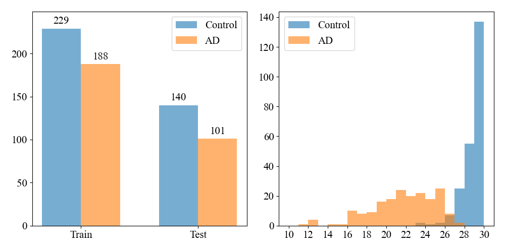
Figure S1: Left: summary of AD vs control in the training and test set; Right: distribution of the MMSE scores, with AD and controls are marked by different colors.

References

Ashburner and Friston, (2005)
Ashburner, J. and Friston, K. J. (2005).
Unified segmentation.
Neuroimage, 26(3):839–851.
Ball et al., (1985)
Ball, M., Hachinski, V., Fox, A., Kirshen, A., Fisman, M., Blume, W., Kral, V.,
Fox, H., and Merskey, H. (1985).
A new definition of alzheimer’s disease: a hippocampal dementia.
The Lancet, 325(8419):14–16.