Local discontinuous Galerkin method for a third order singularly perturbed problem of convection-diffusion type

Abstract

The local discontinuous Galerkin (LDG) method is studied for a third-order singularly perturbed problem of the convection-diffusion type. Based on a regularity assumption for the exact solution, we prove almost $O(N^{-(k+1/2)})$ (up to a logarithmic factor) energy-norm convergence uniformly in the perturbation parameter. Here, $k\geq 0$ is the maximum degree of piecewise polynomials used in discrete space, and $N$ is the number of mesh elements. The results are valid for the three types of layer-adapted meshes: Shishkin-type, Bakhvalov-Shishkin type, and Bakhvalov-type. Numerical experiments are conducted to test the theoretical results.

Keywords: Local discontinuous Galerkin method, Third-order singularly perturbed problem, Convection-diffusion, Shishkin-type mesh, Bakhvalov-type mesh, Uniform convergence

1 Introduction

Singularly perturbed problems have arisen frequently in fluid mechanics, elasticity, chemical reactor theory, and many other related areas [13]. Second- and fourth-order singularly perturbed problems have been widely studied. Only a few results have been reported for third-order singularly perturbed problems, which might come from the theory of dispersive systems and thin-film flows; see the applications described in [7, 8]. Consider the third-order singularly perturbed problem,

$$\begin{split}\varepsilon u^{\prime\prime\prime}(x)-(a(x)u^{\prime}(x))^{\prime}+b(x)u^{\prime}(x)+c(x)u(x)=&f(x)\hskip 10.00002pt{\rm in}\hskip 5.0pt\Omega=(0,1),\\ u(0)=u(1)=u^{\prime}(1)=&0,\end{split}$$ (1)

where $0<\varepsilon\ll 1$ is the perturbation parameter, and $a,b,c,f$ are smooth functions on $\overline{\Omega}$ that satisfy

$$a(x)\geq\alpha>0,\quad c(x)-\frac{1}{2}b^{\prime}(x)\geq\gamma>0,\quad x\in\Omega$$ (2)

for the positive constants $\alpha$ and $\gamma$. The solution to problem (1) typically has a weak boundary layer at $x=1$ (see (5)).

In [12], Roos et al. employed an upwind difference scheme on a Shishkin mesh to solve an analogous third-order singularly perturbed problem. They obtained an almost first-order uniform convergence. In [15], Valarmathi and Ramanujam transformed the third-order equation into a weakly coupled system of first- and second-order equations. An exponentially fitted difference scheme and a classical difference scheme were combined to solve the following two equations in fine and rough domains, respectively. Similarly, in [14], Temsah obtained some numerical results to test the spectral collocation method for the third-order singularly perturbed problem of convection-diffusion type and reaction-diffusion type. As for finite element discretization, Zarin et al. studied a $C^{0}$-continuous interior penalty method and obtained uniform convergence of order $k-1$ in energy-norm for three Shishkin-type meshes [17], where $k>1$ is the highest degree of piecewise polynomials.

This study aims to develop a well-known version of the discontinuous Galerkin (DG) method, i.e. the local discontinuous Galerkin (LDG) method for the problem (1). This method is regarded as a successful application of the DG method to a convection–diffusion system [6]. The main idea is to rewrite the second-order equation into an equivalent first-order system and then apply the DG method to solve each differential equation. The LDG method inherits the advantages of the DG method, such as local conservativity, flexibility with the mesh-design, and the possibility for adaptive $hp$-strategy. Thus, it is suited to problems where solutions have steep gradients or boundary layers. In the past 20 years, there have been extensive studies on LDG methods for solving various equations with higher order derivatives.

For the second order singularly perturbed problem, the LDG method produces good results, even on a uniform mesh; see [3, 16]. In [3, 4], Cheng et al. demonstrated the double-optimal local error estimate of the LDG method on quasi-uniform meshes. In [18, 19], Zhu and Zhang studied the uniform convergence of the LDG method on the standard Shishkin mesh. Recently, the LDG method was applied to solve a two-parameter singularly perturbed problem, and several error estimates were obtained on six types of layer-adapted meshes in a uniform framework [1]. Uniform convergence of the LDG method with generalised alternating numerical fluxes was also obtained for a two-dimensional singularly perturbed convection-diffusion problem [2].

However, we are not aware of any results of the LDG method for third-order singularly perturbed problems. In this paper, we study the LDG method for a third order singularly perturbed problem (1) of convection-diffusion type. In this study, several aspects were addressed.

• Although the LDG method has been studied for many high-order differential equations, no LDG scheme is available in the literature for third-order singularly perturbed problem (1). To construct the LDG scheme, one has to design the numerical fluxes carefully which obey some known principles, such as upwinding for the convective flux, alternating for the diffusive flux, and alternating for the dispersive flux. However, the way to coordinate them suitably, including a suitable setting of these fluxes on the domain boundaries, is unclear. For the first time, in this study, we propose a stable and high-accuracy LDG scheme for problem (1).

• Uniform convergence is often performed for the numerical method on the piecewise uniform Shishkin mesh (S-mesh). However, some generalizations of layer-adapted meshes [10], such as Bakhvalov-Shishkin mesh (BS-mesh) and Bakhvalov-type mesh (B-mesh), are alternatives to eliminate the influence of the logarithmic factor on the convergence rate. In this study, we carry out error analysis on three typical layer-adapted meshes, namely, an S-mesh, a BS-mesh, and a B-mesh. Based on the regularity assumption of the exact solution of (1) and the approximation errors of the local Gauss-Radau projection on the aforementioned layer-adapted meshes [1], we prove an almost optimal energy-norm error estimate of the LDG method on these meshes in a unified framework.

• In the theoretical analysis, we use the local Gauss-Radau projections to address the projection error. However, a difficulty arises from the estimate of the projection error about the second-order derivative. Because we have no stability about this term in the energy-norm of the projection error, we have to seek its control by the first-order derivative as well as the element interface jump of projection error about the primal variable in the energy norm. This relationship can be established from the inherent structure of the LDG scheme. Additionally, to obtain the uniform convergence of the LDG method on the B-mesh, the special structure of this mesh must be studied.

To the best of our knowledge, this is the first uniform-convergence analysis of the LDG method for third-order singularly perturbed problems of convection-diffusion type. These results can also be extended to the third-order problem of reaction-diffusion type, even-order singularly perturbed problems, and higher dimensional problems. This will appear in future work.

The remainder of this paper is organised as follows. In Section 2, we present layer-adapted meshes and describe the LDG method. In Section 3, we carry out the error analysis. Approximation properties of the local Gauss-Radau projections on layer-adapted meshes are presented in Section 3.1 and the main result of the energy-norm error estimate is stated in Section 3.2. In Section 4, we present some numerical experiments to test our theoretical results. Finally, in Section 5 we give our concluding remarks, and in the Appendix we prove a technical lemma.

2 Layer-adapted meshes and the LDG method

Assume that the reduced problem of (1) for $\varepsilon\rightarrow 0$, which is defined as

$$\begin{split}-(a(x)z^{\prime}(x))^{\prime}+b(x)z^{\prime}(x)+c(x)z(x)=&f(x)\hskip 10.00002ptx\in\Omega,\\ z(0)=z(1)=&0\end{split}$$ (3)

is well-defined. Then, for a small $\varepsilon$, problem (1) has a unique solution of the form [11, Theorem 2, Chapter 3]:

$$u(x)=G(x,\varepsilon)+\varepsilon{\tilde{G}}(x,\varepsilon)e^{{\int_{1}^{x}{a(t)dt}}/\varepsilon},$$ (4)

where $G$ and $\tilde{G}$ have asymptotic power-series expansions in $\varepsilon$, $G(x,0)=z(x),x\in[0,1]$. It follows from (4) that

$$|u^{(j)}(x)|\leq C(1+\varepsilon^{-j+1}e^{-\alpha(1-x)/\varepsilon})$$ (5)

for all $x\in\overline{\Omega}$ and $j=0,1,\ldots,\ell$. Here, $\ell$ is some integer that depends on the regularity of the data.

Proposition 1.

[9] Let $\ell$ be a non-negative integer. Assume that the problem (1) has a solution which can be decomposed as $u=\bar{u}+u_{\varepsilon}$, where the regular part $\bar{u}$ and the layer part $u_{\varepsilon}$ satisfy

$$|{\bar{u}}^{(j)}|\leq C,\hskip 70.0001pt|u_{\varepsilon}^{(j)}|\leq C\varepsilon^{1-j}e^{-{\alpha(1-x)}/\varepsilon}$$ (6)

for all $x\in\overline{\Omega}$ and all nonnegative integers $j=0,1,\ldots,\ell$.

In the following analysis, we require $\ell=k+3$ in Proposition 1, where $k$ is the degree of piecewise polynomials in our finite element space.

2.1 Layer-adapted meshes

We shall use the layer-adapted meshes as follows. Let $\varphi:[0,1/2]\to[0,\infty)$ be a mesh-generating function, with $\varphi(0)=0$, which is continuous, piecewise continuously differentiable, and monotonically increasing. Let

$$\tau=\min\Big{\{}\frac{1}{2},\frac{\sigma\varepsilon}{\alpha}\varphi\Big{(}\frac{1}{2}\Big{)}\Big{\}},$$ (7)

where $\sigma>0$ is a constant to be determined. Assume that $\tau=(\sigma\varepsilon/\alpha)\varphi(1/2)$ as is typically the case for (1).

Let $N\geq 2$ be an even integer and $1-\tau$ be a transition point. Partition $\Omega={\Omega^{c}}\cup{\Omega^{f}}$, where $\Omega^{c}=[0,1-\tau]$ is the coarse domain with $N/2$ equidistant elements and $\Omega^{f}=[1-\tau,1]$ is the refined domain with $N/2$ non-uniform elements. The mesh points $\{x_{i}\}_{i=0,1,\dots,N}$ are given by

$$x_{i}=\begin{cases}\frac{2i}{N}(1-\tau)&{\rm for}\hskip 5.0pti=0,1,\ldots,N/2-1,\\ 1-\frac{\sigma\varepsilon}{\alpha}\varphi(1-\frac{i}{N})&{\rm for}\hskip 5.0pti=N/2,N/2+1,\ldots,N.\end{cases}$$ (8)

For varying $\varphi$, we obtain different layer-adapted meshes ; see the Shishkin mesh (S-mesh), Bakhvalov-Shishkin mesh (BS mesh), and the Bakhvalov-type mesh (B-mesh) in Table 1. Here, $\psi=e^{-\varphi}$ is the mesh characterising function, which plays an important role in our convergence analysis.

Table 1: Three layer-adapted meshes.

	$\varphi(t)$	$\min\varphi^{\prime}(t)$	$\max\varphi^{\prime}(t)$	$\psi(t)$	$\max|\psi^{\prime}(t)|$
S-mesh	$2t\ln N$	$2\ln N$	$2\ln N$	$N^{-2t}$	$2\ln N$
BS-mesh	$-\ln[1-2(1-N^{-1})t]$	2	$2N$	$1-2(1-N^{-1})t$	$2$
B-mesh	$-\ln[1-2(1-\varepsilon)t]$	2	2$\varepsilon^{-1}$	$1-2(1-\varepsilon)t$	$2$

Suppose $\varepsilon\leq N^{-1}$, meaning we are in the convection-dominated case. For each mesh type in Table 1, we have $\psi(1/2)\leq N^{-1}$.

Lemma 1.

[2, Lemma 3.1] For any $j=N/2+1,\ldots,N$, we define:

$${\mathcal{G}}_{j}=\min\Big{\{}\frac{h_{j}}{\varepsilon},1\Big{\}}e^{{-\alpha(1-x_{j})}/{\sigma\varepsilon}}.$$

Then, there exists a constant $C>0$ independent of $\varepsilon$ and $N$ such that

$$\max_{N/2+1\leq j\leq N}\mathcal{G}_{j} \leq CN^{-1}\max|\psi^{\prime}|,$$ (9a)

$$\sum_{j={N/2}+1}^{N}{\mathcal{G}}_{j} \leq C.$$ (9b)

Lemma 2.

For the three meshes in Table 1, we have $C\varepsilon N^{-1}\leq h_{j}\leq CN^{-1}$. Moreover, for the B-mesh,

$$h_{N/2+j} \geq\frac{\sigma\varepsilon}{\alpha(j+1)},\quad j=1,2,\dots,N/2,$$ (10a)

$$\sum_{j=N/2+2}^{N}h_{j} \leq C\varepsilon\ln N,$$ (10b)

where $C>0$ is independent of $\varepsilon$ and $N$.

Proof.

It is clear that $N^{-1}\leq h_{j}=2(1-\tau)N^{-1}\leq 2N^{-1}$ for $0\leq j\leq N/2$. For $N/2+1\leq j\leq N$, we have

$$\frac{\sigma\varepsilon}{\alpha}N^{-1}\min\varphi^{\prime}\leq h_{j}\leq\frac{\sigma\varepsilon}{\alpha}N^{-1}\max\varphi^{\prime},$$

which leads to the conclusion $C\varepsilon N^{-1}\leq h_{j}\leq CN^{-1}$ for each types of layer-adapted meshes in Table 1 because $\varepsilon\leq N^{-1}$. In addition, (10a) holds, see [2, Lemma 3.2]. For the B-mesh and $N\geq 2$, one gets

$$\sum_{j=N/2+2}^{N}h_{j}=1-x_{N/2+1}=\frac{\sigma\varepsilon}{\alpha}\varphi\Big{(}\frac{1}{2}-\frac{1}{N}\Big{)}=\frac{\sigma\varepsilon}{\alpha}\ln\Big{(}\frac{N}{2+N\varepsilon-2\varepsilon}\Big{)}\leq\frac{\sigma\varepsilon}{\alpha}\ln\frac{N}{2}\leq C\varepsilon\ln N.$$

This completes the proof of Lemma 2. ∎

2.2 The LDG method

Let $\Omega_{N}:=\{I_{j}=[x_{j-1},x_{j}],j=1,2,\ldots,N\}$ be a partition of $\Omega$ with $x_{0}=0$ and $x_{N}=1$. Let $h_{j}=x_{j}-x_{j-1}$ be the mesh size of the element $I_{j}$, $j=1,2,\ldots,N$. The discontinuous finite element space is defined as

$$\mathcal{V}_{N}=\{v\in L^{2}(\Omega):v|_{I_{j}}\in\mathcal{P}^{k}(I_{j}),j=1,\ldots,N\},$$ (11)

where $\mathcal{P}^{k}(I_{j})$ denotes the space of polynomials in $I_{j}$ of degree at most $k\geq 0$. The functions in $\mathcal{V}_{N}$ allow discontinuity across element interfaces. We denote $v_{j}^{\pm}=\lim_{x\to x_{j}^{\pm}}v(x)$. We define a jump as $[\![v]\!]_{j}=v_{j}^{+}-v_{j}^{-}$ for $j=1,2,\ldots,N-1$, $[\![v]\!]_{0}=v_{0}^{+}$ and $[\![v]\!]_{N}=-v_{N}^{-}$.

Rewrite the problem (1) into an equivalent first-order system

$$p=u^{\prime},\quad q=\varepsilon p^{\prime},\quad q^{\prime}-(ap)^{\prime}+bu^{\prime}+cu=f.$$

Then, the LDG method reads:
Find the numerical solution $\bm{W}=(U,P,Q)\in\mathcal{V}_{N}^{3}:=\mathcal{V}_{N}\times\mathcal{V}_{N}\times\mathcal{V}_{N}$ such that in each element $I_{j}$,

$$\langle P,r\rangle_{I_{j}}+\langle U,r^{\prime}\rangle_{I_{j}}-\hat{U}_{j}r_{j}^{-}+\hat{U}_{j-1}r_{j-1}^{+} =0,$$ (12a)

$$\langle Q,s\rangle_{I_{j}}+\varepsilon(\langle P,s^{\prime}\rangle_{I_{j}}-\hat{P}_{j}s_{j}^{-}+\hat{P}_{j-1}s_{j-1}^{+}) =0,$$ (12b)

$$-\langle Q,v^{\prime}\rangle_{I_{j}}+\hat{Q}_{j}v_{j}^{-}-\hat{Q}_{j-1}v_{j-1}^{+}$$

$$+\langle aP,v^{\prime}\rangle_{I_{j}}-{a_{j}}\tilde{P}_{j}v_{j}^{-}+a_{j-1}\tilde{P}_{j-1}v_{j-1}^{+}$$

$$-\langle bU,v^{\prime}\rangle_{I_{j}}+\widetilde{bU}_{j}v_{j}^{-}-\widetilde{bU}_{j-1}v_{j-1}^{+}+\langle(c-b^{\prime})U,v\rangle_{I_{j}} =\langle f,v\rangle_{I_{j}}$$ (12c)

hold for any test function $\bm{\chi}=(v,r,s)\in\mathcal{V}_{N}^{3}$, where $\langle\cdot,\cdot\rangle_{I_{j}}$ is the inner product in ${L^{2}}(I_{j})$, the ”hat” terms and ”tilde” terms are the numerical fluxes defined in Table 2.

Table 2: Numerical fluxes in (12)

	$j=1,2,\dots,N-1$		$j=0$		$j=N$
$\hat{U}_{j}$	$U^{-}_{j}$		$0$		$0$
$\hat{P}_{j}$	$P^{+}_{j}$		$P^{+}_{0}$		$0$
$\hat{Q}_{j}$	$Q^{+}_{j}$		$Q^{+}_{0}$		$Q^{-}_{N}$
$\tilde{P}_{j}$	$P^{+}_{j}$		$P^{+}_{0}$		$P^{-}_{N}$
$\widetilde{bU}_{j}$	$\frac{b_{j}+|b_{j}|}{2}U_{j}^{-}+\frac{b_{j}-|b_{j}|}{2}U_{j}^{+}$		$\frac{b_{0}-|b_{0}|}{2}U_{0}^{+}$		$\frac{b_{N}+|b_{N}|}{2}U_{N}^{-}$

Note that at the interior element boundary points, we choose an upwind flux for the convection part $\widetilde{bU}$, an alternating flux for the diffusion part $(\hat{U}_{j},\tilde{P}_{j})$, and the dispersive part $(\hat{U}_{j},\hat{Q}_{j})$. The choice of flux $\hat{P}_{j}$ ensures stability of the numerical scheme. This completes the definition of the LDG method for problem (1).

Denoting by $\langle w,v\rangle=\sum_{j=1}^{N}\langle w,v\rangle_{I_{j}}$, we can rewrite the above-mentioned LDG method in a compact form:
Find ${\bm{W}}=(U,P,Q)\in\mathcal{V}_{N}^{3}$, such that

$$B(\bm{W};\bm{\chi})=\langle f,v\rangle\hskip 20.00003pt\forall\bm{\chi}=(v,r,s)\in\mathcal{V}_{N}^{3},$$ (13)

where

$$B(\bm{W};\bm{\chi}) =\langle P,r\rangle+\langle U,r^{\prime}\rangle+\sum_{j=1}^{N-1}U_{j}^{-}[\![r]\!]_{j}$$

$$+\langle Q,s\rangle+\varepsilon\left(\langle P,s^{\prime}\rangle+\sum_{j=1}^{N-1}P_{j}^{+}[\![s]\!]_{j}+P_{0}^{+}s_{0}^{+}\right)$$

$$-\langle Q,v^{\prime}\rangle-\sum_{j=1}^{N-1}Q_{j}^{+}[\![v]\!]_{j}+Q_{N}^{-}v_{N}^{-}-Q_{0}^{+}v_{0}^{+}$$ (14)

$$+\langle aP,v^{\prime}\rangle+\sum_{j=1}^{N-1}a_{j}P_{j}^{+}[\![v]\!]_{j}-a_{N}P_{N}^{-}v_{N}^{-}+a_{0}P_{0}^{+}v_{0}^{+}$$

$$+\langle(c-b^{\prime})U,v\rangle-\langle bU,v^{\prime}\rangle-\sum_{j=1}^{N-1}\left(\frac{b_{j}+|b_{j}|}{2}U_{j}^{-}+\frac{b_{j}-|b_{j}|}{2}U_{j}^{+}\right)[\![v]\!]_{j}$$

$$+\frac{b_{N}+|b_{N}|}{2}U_{N}^{-}v_{N}^{-}-\frac{b_{0}-|b_{0}|}{2}U_{0}^{+}v_{0}^{+}.$$

By integrating parts and making trivial manipulations, one arrives at the energy norm

$$\begin{split}\interleave\bm{W}\interleave^{2}&:=B(U,P,Q;U,-Q+aP,P)\\ &=\frac{\varepsilon}{2}\sum_{j=0}^{N}[\![P]\!]_{j}^{2}+\|a^{1/2}P\|^{2}+\|(c-{b^{\prime}/2)}^{1/2}U\|^{2}+\frac{1}{2}\sum_{j=0}^{N}|b_{j}|[\![U]\!]_{j}^{2},\end{split}$$

which implies the existence and uniqueness of numerical solution defined by (13), because $U=P=Q=0$ if $f=0$ and $\bm{\chi}$ is taken suitably in (13).

3 Error analysis

This section focuses on the error estimate in the energy norm (2.2). We denote the error by $\bm{e}=(u-U,p-P,q-Q)$ and split it into two parts: $\bm{e}=\bm{w}-\bm{W}=(\bm{w}-\bm{\Pi w})-(\bm{W}-\bm{\Pi w}):=\bm{\eta-\xi}$ with

$$\bm{\eta} =(\eta_{u},\eta_{p},\eta_{q})=(u-\pi^{-}u,p-\pi^{+}p,q-\pi^{+}q),$$ (15a)

$$\bm{\xi} =(\xi_{u},\xi_{p},\xi_{q})=(U-\pi^{-}u,P-\pi^{+}p,Q-\pi^{+}q)\in\mathcal{V}_{N}^{3},$$ (15b)

where $\bm{\Pi w}:=(\pi^{-}u,\pi^{+}p,\pi^{+}q):(H^{1}(\Omega_{N}))^{3}\to\mathcal{V}_{N}^{3}$ denotes the local Gauss-Radau projection that will be defined below.

In Section 3.1, we present an estimation of approximation error $\bm{\eta}$. Then, we utilise its property to derive the bound of the projection error $\bm{\xi}$ and, hence, the error $\bm{e}$ in Section 3.2.

3.1 The approximation error

To derive the error estimate, we use local Gauss-Radau projections $\pi^{\pm}$, defined as follows. For any $z\in H^{1}(\Omega_{N})$, we have $\pi^{\pm}z\in\mathcal{V}_{N}$ satisfies

$$\langle\pi^{+}z,v\rangle_{I_{j}} \;=\langle z,v\rangle_{I_{j}}\quad\forall v\in{\mathcal{P}}^{k-1}(I_{j}),\quad(\pi^{+}z)_{j-1}^{+}=z_{j-1}^{+};$$

$$\langle\pi^{-}z,v\rangle_{I_{j}} \;=\langle z,v\rangle_{I_{j}}\quad\forall v\in{\mathcal{P}}^{k-1}(I_{j}),\quad(\pi^{-}z)_{j}^{-}=z_{j}^{-}$$ (16)

on each element $I_{j}=[x_{j-1},x_{j}]$, $j=1,2,\ldots,N$. From [5], one could verify the existence and uniqueness of these projections. Furthermore, denote $\|v\|_{I_{j}}=\|v\|_{L^{2}(I_{j})}$ and $\|v\|_{L^{\infty}(I_{j})}$ for the typical $L^{2}$ and $L^{\infty}$ norms on $I_{j}$ respectively; then, one obtains the following properties

$$\|\pi^{-}z\|_{I_{j}} \leq C[\|z\|_{I_{j}}+h_{j}^{1/2}|z^{-}_{j}|],$$ (17a)

$$\|\pi^{+}z\|_{I_{j}} \leq C[\|z\|_{I_{j}}+h_{j}^{1/2}|z^{+}_{j-1}|],$$ (17b)

$$\|\pi^{\pm}z\|_{L^{\infty}(I_{j})} \leq C\|z\|_{L^{\infty}(I_{j})},$$ (17c)

$$\|z-\pi^{\pm}z\|_{L^{\ell}(I_{j})} \leq Ch_{j}^{k+1}\|z^{(k+1)}\|_{L^{\ell}(I_{j})},\hskip 20.00003pt\ell=2,\infty,$$ (17d)

where $C>0$ is independent of the element size $h_{j}$ and function $z$.

Lemma 3.

Let $\Omega_{N}$ be a layer-adapted mesh (8) with $\sigma\geq k+1.5$. For the function $u$ satisfying Proposition 1, we have

$$\|u-\pi^{-}u\| \leq C\Big{[}\varepsilon{(N^{-1}\max|\psi^{\prime}|)}^{k+1}+N^{-(k+1)}\Big{]},$$ (18a)

$$\|p-\pi^{+}p\| \leq C\Big{[}\sqrt{\varepsilon}{(N^{-1}\max|\psi^{\prime}|)}^{k+1}+N^{-(k+1)}\Big{]},$$ (18b)

$$\|q-\pi^{+}q\| \leq C\sqrt{\varepsilon}(N^{-1}\max|\psi^{\prime}|)^{k+1},$$ (18c)

$$\|p-\pi^{+}p\|_{L^{\infty}(\Omega^{f})} \leq C(N^{-1}\max|\psi^{\prime}|)^{k+1},$$ (18d)

$$\|q-\pi^{+}q\|_{L^{\infty}(\Omega^{f})} \leq C(N^{-1}\max|\psi^{\prime}|)^{k+1},$$ (18e)

$$\left(\sum_{j=0}^{N}[\![u-\pi^{-}u]\!]^{2}_{j}\right)^{1/2} \leq C\left[\varepsilon(N^{-1}\max|\psi^{\prime}|)^{k+1/2}+N^{-(k+1/2)}\right],$$ (18f)

$$\left(\sum_{j=0}^{N}[\![p-\pi^{+}p]\!]^{2}_{j}\right)^{1/2} \leq C(N^{-1}\max|\psi^{\prime}|)^{k+1/2},$$ (18g)

where $p=u^{\prime}$, $q=\varepsilon u^{\prime\prime}$ and $C>0$ is independent of $\varepsilon$ and $N$.

Proof.

We would like to show these inequalities individually. The main idea is to fully use the stability and approximation properties (17) for the function $u$ satisfying Proposition 1.

(1)We first show (18a). For notational simplification, we denote $\eta_{u_{z}}=u_{z}-\pi^{-}u_{z}$ for $u_{z}\in\{\bar{u},u_{\varepsilon}\}$. Using (17d) for the regular part $\bar{u}$ yields:

$$\|\eta_{\bar{u}}\|^{2}=\sum_{j=1}^{N}\|\eta_{\bar{u}}\|_{I_{j}}^{2}\leq C\sum_{j=1}^{N}h_{j}^{2(k+1)}\|{\bar{u}}^{(k+1)}\|_{I_{j}}^{2}\leq CN^{-2(k+1)}$$ (19)

because $h_{j}\leq CN^{-1}(j=1,2,\ldots,N)$ from Lemma 2.

To bound the approximation error for the layer component $u_{\varepsilon}$, we proceed as follows. First, using (17a) and (6), we get

$$\sum_{j=1}^{N/2}\|\eta_{u_{\varepsilon}}\|_{I_{j}}^{2} \leq C\sum_{j=1}^{N/2}\left[\|u_{\varepsilon}\|_{I_{j}}^{2}+N^{-1}|u_{\varepsilon}(x_{j})|^{2}\right]$$

$$\leq C\int_{0}^{1-\tau}\varepsilon^{2}e^{{-2\alpha(1-x)}/{\varepsilon}}dx+CN^{-1}\varepsilon^{2}e^{{-2\alpha(1-x_{N/2})}/{\varepsilon}}$$

$$\leq C\varepsilon^{2}(\varepsilon+N^{-1})N^{-2\sigma},$$ (20)

where we used $\psi(1/2)\leq N^{-1}$. Second, using $h_{j}\leq CN^{-1}(j=1,2,\ldots,N)$, (17c) and (17d) along with $\sigma\geq k+1$, we obtain

$$\sum_{j=N/2+1}^{N}\|\eta_{u_{\varepsilon}}\|_{I_{j}}^{2} \leq CN^{-1}\sum_{j=N/2+1}^{N}\|u_{\varepsilon}-\pi^{-}{u_{\varepsilon}}\|_{{L^{\infty}}(I_{j})}^{2}$$

$$\leq CN^{-1}\sum_{j=N/2+1}^{N}\min\Big{\{}\|u_{\varepsilon}\|_{{L^{\infty}}(I_{j})}^{2},h_{j}^{2(k+1)}\|u_{\varepsilon}^{(k+1)}\|_{{L^{\infty}}(I_{j})}^{2}\Big{\}}$$

$$\leq CN^{-1}\varepsilon^{2}\sum_{j=N/2+1}^{N}\Big{(}\min\Big{\{}\frac{h_{j}}{\varepsilon},1\Big{\}}e^{{-\alpha(1-{x_{j}})}/{\sigma\varepsilon}}\Big{)}^{2(k+1)}$$

$$\leq CN^{-1}\varepsilon^{2}\max_{N/2+1\leq j\leq N}\mathcal{G}_{j}^{2k+1}\sum_{j=N/2+1}^{N}\mathcal{G}_{j}$$

$$\leq C\varepsilon^{2}N^{-1}\Big{(}N^{-1}\max|\psi^{\prime}|\Big{)}^{2k+1},$$ (21)

where (9a)-(9b) were used. Consequently, $\|\eta_{u}\|$ follows from (19)-(3.1), triangle inequality and $\sigma\geq k+1$.

(2) We next show (18b) and (18c). Denote $p=\bar{p}+{p_{\varepsilon}}:=\bar{u}^{\prime}+u^{\prime}_{\varepsilon}$, where $|\bar{p}^{(j)}|\leq C$ and $|p_{\varepsilon}^{(j)}|\leq C\varepsilon^{-j}e^{-\alpha(1-x)/\varepsilon}$ for $j\leq k+1$. Let $\eta_{p_{z}}=p_{z}-\pi^{+}p_{z}$ for $p_{z}\in\{\bar{p},p_{\varepsilon}\}$.

Evidently $\|\eta_{\bar{p}}\|\leq\|\eta_{\bar{p}}\|_{L^{\infty}(\Omega_{N})}\leq CN^{-(k+1)}$. Projection $\pi^{+}$ has good stability for the monotone increasing function $x\mapsto e^{-\alpha(1-x)/\varepsilon}$, which results in layer approximation in the rough region to satisfy

$$\sum_{j=1}^{N/2}\|\eta_{p_{\varepsilon}}\|_{I_{j}}^{2} \leq C\sum_{j=1}^{N/2}\left[\|p_{\varepsilon}\|_{I_{j}}^{2}+h_{j}|p_{\varepsilon}(x_{j-1})|^{2}\right]\leq C\sum_{j=1}^{N/2}\left[\|e^{{-\alpha(1-x)}/\varepsilon}\|_{I_{j}}^{2}+h_{j}e^{{-2\alpha(1-x_{j-1})}/\varepsilon}\right]$$

$$\leq C\int_{0}^{1-\tau}e^{{-2\alpha(1-x)}/{\varepsilon}}dx\leq C\varepsilon N^{-2\sigma}.$$ (22)

Hence, for $\sigma\geq k+1$ we get

$$\|\eta_{p}\|_{\Omega^{c}}\leq C\Big{[}\|\eta_{p_{\varepsilon}}\|_{\Omega^{c}}+\|\eta_{\bar{p}}\|_{\Omega^{c}}\Big{]}\leq C\left[N^{-(k+1)}+\sqrt{\varepsilon}N^{-\sigma}\right]\leq CN^{-(k+1)}.$$ (23)

The proof is similar as in (3.1), for a larger $\sigma\geq k+1.5$, one bounds the layer approximation in the fine region by

$$\sum_{j=N/2+1}^{N}\|\eta_{p_{\varepsilon}}\|_{I_{j}}^{2} \leq C\sum_{j={N/2+1}}^{N}\min\Big{\{}h_{j}^{2(k+1)}\|{p_{\varepsilon}}^{(k+1)}\|_{I_{j}}^{2},h_{j}\big{|}p_{\varepsilon}(x_{j-1})\big{|}^{2}+\|p_{\varepsilon}\|_{I_{j}}^{2}\Big{\}}$$

$$\leq C\sum_{j=N/2+1}^{N}\min\Big{\{}{\Big{(}\frac{h_{j}}{\varepsilon}\Big{)}}^{2(k+1)},1\Big{\}}\|e^{{-\alpha(1-x)}/{\varepsilon}}\|_{I_{j}}^{2}$$

$$\leq C\sum_{j=N/2+1}^{N}\varepsilon\Big{(}\min\Big{\{}{\frac{h_{j}}{\varepsilon},1}\Big{\}}e^{{-\alpha(1-{x_{j}})}/{\sigma\varepsilon}}\Big{)}^{2(k+{3/2})}$$

$$\leq C\varepsilon\max_{N/2+1\leq j\leq N}{\mathcal{G}_{j}}^{2(k+1)}\sum_{j=N/2+1}^{N}\mathcal{G}_{j}\leq C\varepsilon(N^{-1}\max|\psi^{\prime}|)^{2(k+1)}.$$ (24)

Hence, we get

$$\|\eta_{p}\|_{\Omega^{f}}\leq C\Big{[}\|\eta_{p_{\varepsilon}}\|_{\Omega^{f}}+\|\eta_{\bar{p}}\|_{\Omega^{f}}\Big{]}\leq C\left[\sqrt{\varepsilon}(N^{-1}\max|\psi^{\prime}|)^{(k+1)}+|\Omega^{f}|^{1/2}N^{-(k+1)}\right].$$ (25)

Due to (23) and (25), so (18b) is proved. In a similar fashion, (18c) can be proved.

(3) We now show (18d) and (18e). This follows from stability and approximation property of $\pi^{+}$ under $L^{\infty}$norm. For example, for each element $I_{j}$,

$$\|\eta_{\bar{p}}\|_{{L^{\infty}}(I_{j})}\leq CN^{-(k+1)}\|{\bar{p}}^{(k+1)}\|_{{L^{\infty}}(I_{j})}\leq CN^{-(k+1)}.$$

When $j=N/2+1,\ldots,N$, using (17c), (17d) and (9a), we get

$$\|\eta_{p_{\varepsilon}}\|_{{L^{\infty}}(I_{j})} \leq C\min\Big{\{}\|p_{\varepsilon}\|_{{L^{\infty}}(I_{j})},h_{j}^{k+1}\|p_{\varepsilon}^{(k+1)}\|_{{L^{\infty}}(I_{j})}\Big{\}}$$

$$\leq C{\mathcal{G}_{j}}^{k+1}\leq C(N^{-1}\max|\psi^{\prime}|)^{k+1}.$$ (26)

This immediately leads to (18d). Analogously, we can prove (18e).

(4)We then present (18f). From $L^{\infty}$approximation property (17d) and (6), we have

$$\sum_{j=0}^{N}[\![\eta_{\bar{u}}]\!]_{j}^{2}\leq C\sum_{j=1}^{N}\|\eta_{\bar{u}}\|_{{L^{\infty}}(I_{j})}^{2}\leq C\sum_{j=1}^{N}N^{-2(k+1)}\leq CN^{-(2k+1)}.$$

Using Lemma 1 and (17c), (17d) with $\ell=\infty$, Proposition 1 and $\sigma\geq k+1$, we get

$$\sum_{j=0}^{N}[\![\eta_{u_{\varepsilon}}]\!]_{j}^{2} \leq C\sum_{j=1}^{N/2}\|\eta_{u_{\varepsilon}}\|_{{L^{\infty}}(I_{j})}^{2}+C\sum_{j=N/2+1}^{N}\|\eta_{u_{\varepsilon}}\|_{{L^{\infty}}(I_{j})}^{2}$$

$$\leq C\sum_{j=1}^{N/2}\|u_{\varepsilon}\|_{{L^{\infty}}(I_{j})}^{2}+C\sum_{j=N/2+1}^{N}\min\Big{\{}\|u_{\varepsilon}\|^{2}_{{L^{\infty}}(I_{j})},h_{j}^{2(k+1)}\|u_{\varepsilon}^{(k+1)}\|^{2}_{{L^{\infty}}(I_{j})}\Big{\}}$$

$$\leq C\varepsilon^{2}N^{-2\sigma+1}+C\varepsilon^{2}\max_{N/2+1\leq j\leq N}{\mathcal{G}_{j}}^{2k+1}\sum_{j=N/2+1}^{N}\mathcal{G}_{j}$$

$$\leq C\varepsilon^{2}(N^{-1}\max|\psi^{\prime}|)^{2k+1}.$$ (27)

Consequently, (18f) follows.

(5) We finally show (18g). The proof is similar as in (18f). In fact, one has

$$\sum_{j=0}^{N}[\![\eta_{p}]\!]_{j}^{2} \leq C\sum_{j=1}^{N}\|\eta_{\bar{p}}\|_{{L^{\infty}}(I_{j})}^{2}+C\sum_{j=1}^{N}\|\eta_{p_{\varepsilon}}\|_{{L^{\infty}}(I_{j})}^{2}$$

$$\leq CN^{-(2k+1)}+CN^{-2\sigma+1}+C\max_{N/2+1\leq j\leq N}{\mathcal{G}_{j}}^{2k+1}\sum_{j=N/2+1}^{N}\mathcal{G}_{j}$$

$$\leq C(N^{-1}\max|\psi^{\prime}|)^{2k+1}.$$

This completes the whole proof of this lemma. ∎

3.2 Main result

We obtain the following energy-norm error estimate:

Theorem 1.

Let $\bm{w}=(u,p,q)=(u,u^{\prime},\varepsilon u^{\prime\prime})$ be the exact solution of problem (1) satisfying Proposition 1 and $\bm{W}=(U,P,Q)\in{\mathcal{V}}_{N}^{3}$ be the numerical solution of the LDG scheme (13) on the three layer-adapted meshes of Table 1 with $\sigma\geq k+1.5$. Then, we have

$$\interleave\bm{w}-\bm{W}\interleave\leq\begin{cases}C\left(\sqrt{\varepsilon}(N^{-1}\ln N)^{k}+(N^{-1}\ln N)^{k+1}+N^{-(k+1/2)}\right)&\text{for S-mesh,}\\ C\left(\sqrt{\varepsilon}N^{-k}(\ln N)^{1/2}+N^{-(k+1/2)}\right)&\text{for BS-mesh and B-mesh,}\end{cases}$$ (28)

where $C>0$ is a constant independent of $\varepsilon$ and $N$.

Proof.

Recalling $\bm{\eta}=\bm{w}-\bm{\Pi}\bm{w}$ and $\bm{\xi}=\bm{W}-\bm{\Pi}\bm{w}$. Owing to Galerkin orthogonality $B(\bm{w}-\bm{W};\bm{\chi})=0\quad\forall\bm{\chi}\in\mathcal{V}_{N}^{3}$, we have the following error equation:

$$B(\bm{\xi;\bm{\chi}})=B(\bm{\eta;\bm{\chi}})\hskip 20.00003pt\forall\bm{\chi}=(v,r,s)\in\mathcal{V}_{N}^{3}.$$ (29)

Taking $\bm{\chi}=(\xi_{u},-\xi_{q}+a\xi_{p},\xi_{p})$ in (29), one has

$$B(\bm{\eta;\bm{\chi}}):=\sum_{i=1}^{12}{S_{i}},$$ (30)

where

$$S_{1}:= (\eta_{p},-\xi_{q}+a\xi_{p});\hskip 5.0ptS_{2}:=(\eta_{u},-\xi^{\prime}_{q}+{(a\xi_{p})}^{\prime});\hskip 5.0ptS_{3}:=\sum_{j=1}^{N-1}(\eta_{u})_{j}^{-}[\![-\xi_{q}+a\xi_{p}]\!]_{j};$$

$$S_{4}:= (\eta_{q},\xi_{p});\hskip 30.00005ptS_{5}:=\varepsilon(\eta_{p},\xi^{\prime}_{p});\hskip 20.00003ptS_{6}:=\varepsilon\sum_{j=1}^{N-1}(\eta_{p})_{j}^{+}[\![\xi_{p}]\!]_{j}+\varepsilon(\eta_{p})_{0}^{+}(\xi_{p})_{0}^{+};$$

$$S_{7}:= -(\eta_{q},\xi^{\prime}_{u});\hskip 20.00003ptS_{8}:=-\sum_{j=1}^{N-1}(\eta_{q})_{j}^{+}[\![\xi_{u}]\!]_{j}+(\eta_{q})_{N}^{-}(\xi_{u})_{N}^{-}-(\eta_{q})_{0}^{+}(\xi_{u})_{0}^{+};$$

$$S_{9}:= (a\eta_{p},\xi^{\prime}_{u});\hskip 20.00003ptS_{10}:=\sum_{j=1}^{N-1}a_{j}(\eta_{p})_{j}^{+}[\![\xi_{u}]\!]_{j}-a_{N}(\eta_{p})_{N}^{-}(\xi_{u})_{N}^{-}+a_{0}(\eta_{p})_{0}^{+}(\xi_{u})_{0}^{+};$$

$$S_{11}:= ((c-b^{\prime})\eta_{u},\xi_{u})-(b\eta_{u},\xi^{\prime}_{u});$$

$$S_{12}:= -\sum_{j=1}^{N-1}\left(\frac{b_{j}+|b_{j}|}{2}(\eta_{u})_{j}^{-}+\frac{b_{j}-|b_{j}|}{2}(\eta_{u})_{j}^{+}\right)[\![\xi_{u}]\!]_{j}$$

$$+\frac{b_{N}+|b_{N}|}{2}(\eta_{u})_{N}^{-}(\xi_{u})_{N}^{-}-\frac{b_{0}-|b_{0}|}{2}(\eta_{u})_{0}^{+}(\xi_{u})_{0}^{+}.$$

From the orthogonality of the approximating polynomials and the exact collocation of the Gauss-Radau projection, it is easy to find that

$$S_{3}=S_{5}=S_{6}=S_{7}=0.$$ (31)

Using the Cauchy-Schwarz inequality, inverse inequality, the definition (3.1) of the Gauss-Radau projection and $a\geq\alpha>0$, we obtain

$$|S_{2}| =|(\eta_{u},(a-\bar{a})\xi^{\prime}_{p})+(\eta_{u},a^{\prime}\xi_{p})|$$

$$\leq\sum_{j=1}^{N}\left(\|\eta_{u}\|_{I_{j}}\cdot h_{j}\|a^{\prime}\|_{{L^{\infty}}(I_{j})}\cdot Ch_{j}^{-1}\|\xi_{p}\|_{I_{j}}\right)+C\|\eta_{u}\|\|a^{1/2}\xi_{p}\|$$

$$\leq C\|\eta_{u}\|\|a^{1/2}\xi_{p}\|\leq C\|\eta_{u}\|\interleave\bm{\xi}\interleave\leq C\|\eta_{u}\|^{2}+\frac{1}{28}\interleave\bm{\xi}\interleave^{2},$$ (32)

where $\bar{a}$ is a piecewise constant function defined by $\bar{a}=\frac{1}{h_{j}}\int_{I_{j}}a\rm dx$ on each element $I_{j}$.

Analogously, one has

$$|S_{4}| \leq\|\eta_{q}\|\|\xi_{p}\|\leq C\|\eta_{q}\|^{2}+\frac{1}{28}\interleave\bm{\xi}\interleave^{2},$$ (33)

$$|S_{8}| =|(\eta_{q})_{N}^{-}(\xi_{u})_{N}^{-}|\leq C\|\eta_{q}\|_{{L^{\infty}}(\Omega^{f})}^{2}+\frac{1}{28}\interleave\bm{\xi}\interleave^{2},$$ (34)

$$|S_{9}| =|((a-\bar{a})\eta_{p},\xi^{\prime}_{u})|\leq C\|\eta_{p}\|\interleave\bm{\xi}\interleave\leq C\|\eta_{p}\|^{2}+\frac{1}{28}\interleave\bm{\xi}\interleave^{2},$$ (35)

$$|S_{10}| =|-a_{N}(\eta_{p})_{N}^{-}(\xi_{u})_{N}^{-}|\leq C\|\eta_{p}\|_{{L^{\infty}}(\Omega^{f})}^{2}+\frac{1}{28}\interleave\bm{\xi}\interleave^{2},$$ (36)

$$|S_{11}| =|((c-b^{\prime})\eta_{u},\xi_{u})+((\bar{b}-b)\eta_{u},\xi^{\prime}_{u})|$$

$$\leq C\left\|{{\eta_{u}}}\right\|\interleave\bm{\xi}\interleave_{E}\leq C\|\eta_{u}\|^{2}+\frac{1}{28}\interleave\bm{\xi}\interleave^{2}.$$ (37)

To bound $S_{12}$, we note that $(\eta_{u})_{j}^{-}=0$ for $j=1,2,\dots,N$, $(\eta_{u})_{j}^{+}=[\![\eta_{u}]\!]_{j}$ for $j=0,1,\dots,N-1$ and

$$\left|\frac{b_{j}-|b_{j}|}{2}(\eta_{u})_{j}^{+}[\![\xi_{u}]\!]_{j}\right|\leq|[\![\eta_{u}]\!]_{j}|(|b_{j}||[\![\xi_{u}]\!]_{j}|).$$

Using the Cauchy-Schwarz inequality, we obtain

$$|S_{12}| =\left|-\sum_{j=0}^{N-1}\frac{b_{j}-|b_{j}|}{2}(\eta_{u})_{j}^{+}[\![\xi_{u}]\!]_{j}\right|\leq\sqrt{2}\left(\sum_{j=0}^{N-1}[\![\eta_{u}]\!]_{j}^{2}\right)^{1/2}\left(\sum_{j=0}^{N-1}\frac{1}{2}|b_{j}|[\![\xi_{u}]\!]_{j}^{2}\right)^{1/2}$$

$$\leq C\sum_{j=0}^{N}[\![\eta_{u}]\!]_{j}^{2}+\frac{1}{28}\interleave\bm{\xi}\interleave^{2}.$$ (38)

Finally, we bound $S_{1}$. The main challenge is to bound $\|\xi_{q}\|$ which is not included in the energy norm $\interleave\bm{\xi}\interleave$. We intend to seek its control by $\|\xi_{p}\|$ and $\left(\frac{\varepsilon}{2}\sum_{j=1}^{N}[\![\xi_{p}]\!]_{j}^{2}\right)^{1/2}$. This depends on the inherent structure of the LDG scheme, as we shall describe. Taking $v=r=0$ in (29) and restricting the test function $s$ to the local element $I_{j}$, we have that

$$\langle\xi_{q},s\rangle_{I_{j}}+\varepsilon\Big{(}\langle\xi_{p},s^{\prime}\rangle_{I_{j}}-(\hat{\xi}_{p})_{j}s_{j}^{-}+(\hat{\xi}_{p})_{j-1}s_{j-1}^{+}\Big{)}=\langle\eta_{q},s\rangle_{I_{j}}$$

in each element $I_{j}$ for any function $s\in\mathcal{P}^{k}(I_{j})$, where we use the property of $\eta_{p}=p-\pi^{+}p$. Thus, $(\xi_{p},\xi_{q})\in\mathcal{V}^{2}_{N}$ satisfies (A.1), with $F_{j}(s)=(\eta_{q},s)_{I_{j}}$. From (A.2), we have

$$\|\xi_{q}\|_{I_{j}}\leq C\varepsilon\left(h_{j}^{-1}\|\xi_{p}\|_{I_{j}}+h_{j}^{-1/2}|[\![\xi_{p}]\!]_{j}|\right)+\|\eta_{q}\|_{I_{j}}$$ (39)

for $j=1,2,\dots,N$. Using the Cauchy-Schwarz and Young’s inequalities, yields

$$|(\eta_{p},-\xi_{q})| \leq\sum_{j=1}^{N}\|\eta_{p}\|_{I_{j}}\|\xi_{q}\|_{I_{j}}$$

$$\leq C\sum_{j=1}^{N}\|\eta_{p}\|_{I_{j}}\left(\varepsilon h_{j}^{-1}\|\xi_{p}\|_{I_{j}}+\varepsilon h_{j}^{-1/2}|[\![\xi_{p}]\!]_{j}|+\|\eta_{q}\|_{I_{j}}\right)$$

$$\leq C\sum_{j=1}^{N}\left(1+\frac{\varepsilon}{h_{j}}\right)^{2}\|\eta_{p}\|^{2}_{I_{j}}+\frac{1}{8}\|a^{1/2}\xi_{p}\|^{2}+\frac{1}{4}\cdot\frac{\varepsilon}{2}\sum_{j=1}^{N}[\![\xi_{p}]\!]_{j}^{2}+C\|\eta_{q}\|^{2}.$$

So, one gets

$$\begin{split}|S_{1}|\leq&|\langle\eta_{p},-\xi_{q}\rangle|+C\|\eta_{p}\|^{2}+\frac{1}{8}\|a^{1/2}\xi_{p}\|^{2}\leq C\sum_{j=1}^{N}\left(1+\frac{\varepsilon}{h_{j}}\right)^{2}\|\eta_{p}\|^{2}_{I_{j}}+C\|\eta_{q}\|^{2}+\frac{1}{4}\interleave\bm{\xi}\interleave^{2}.\end{split}$$ (40)

Collecting the above estimates, we get

$$\interleave\bm{\xi}\interleave^{2}\leq C\left[\sum_{j=1}^{N}\left(1+\frac{\varepsilon}{h_{j}}\right)^{2}\|\eta_{p}\|^{2}_{I_{j}}+\|\eta_{u}\|^{2}+\|\eta_{q}\|^{2}+\sum_{j=0}^{N}[\![\eta_{u}]\!]_{j}^{2}+\|\eta_{p}\|_{{L^{\infty}}(\Omega^{f})}^{2}+\|\eta_{q}\|_{{L^{\infty}}(\Omega^{f})}^{2}\right].$$ (41)

In the sequel, we shall estimate the first term on the right hand side of (41) for each type of layer-adapted meshes. For S-mesh, one uses (23) and (25) to get that

$$\sum_{j=1}^{N}\left(1+\frac{\varepsilon}{h_{j}}\right)^{2}\|\eta_{p}\|^{2}_{I_{j}}\leq \;C(1+\varepsilon N)^{2}\|\eta_{p}\|^{2}_{\Omega^{c}}+C(1+N(\ln N)^{-1})^{2}\|\eta_{p}\|^{2}_{\Omega^{f}}$$

$$\leq \;C(1+\varepsilon N)^{2}N^{-2(k+1)}+C\left(N(\ln N)^{-1}\right)^{2}\left[\varepsilon(N^{-1}\ln N)^{2(k+1)}+\varepsilon N^{-2(k+1)}\ln N\right]$$

$$\leq \;C\varepsilon(N^{-1}\ln N)^{2k}+CN^{-2(k+1)}.$$

For BS-mesh, using Lemma 2, (23) and (25), we have

$$\sum_{j=1}^{N}\left(1+\frac{\varepsilon}{h_{j}}\right)^{2}\|\eta_{p}\|^{2}_{I_{j}}\leq \;C(1+\varepsilon N)^{2}\|\eta_{p}\|^{2}_{\Omega^{c}}+CN^{2}\|\eta_{p}\|^{2}_{\Omega^{f}}\leq C\varepsilon N^{-2k}\ln N+CN^{-2(k+1)}.$$

For B-mesh, we obtain from Lemma 2, (23) and (18d) that

$$\sum_{j=1}^{N}\left(1+\frac{\varepsilon}{h_{j}}\right)^{2}\|\eta_{p}\|^{2}_{I_{j}}\leq \;C(1+\varepsilon N)^{2}\|\eta_{p}\|^{2}_{\Omega^{c}}+\sum_{j=N/2+2}^{N}\left(1+\frac{\varepsilon}{h_{j}}\right)^{2}\|\eta_{p}\|^{2}_{I_{j}}+\left(1+\frac{\varepsilon}{h_{N/2+1}}\right)^{2}\|\eta_{p}\|^{2}_{I_{N/2+1}}$$

$$\leq \;C(1+\varepsilon N)^{2}\|\eta_{p}\|^{2}_{\Omega^{c}}+CN^{2}\left(\sum_{j=N/2+2}^{N}h_{j}\right)\|\eta_{p}\|^{2}_{L^{\infty}(\Omega^{f})}+C\|\eta_{p}\|^{2}$$

$$\leq \;C\varepsilon N^{-2k}\ln N+CN^{-2(k+1)}.$$

Inserting the above estimates into (41) and using Lemma 3, we have

$$\interleave\bm{\xi}\interleave^{2}\leq\begin{cases}C\left(\varepsilon(N^{-1}\ln N)^{2k}+(N^{-1}\ln N)^{2(k+1)}+N^{-(2k+1)}\right)&\text{for S-mesh,}\\ C\left(\varepsilon N^{-2k}\ln N+N^{-(2k+1)}\right)&\text{for BS-mesh and B-mesh.}\\ \end{cases}$$ (42)

Theorem 1 follows from (42), Lemma 3 and triangle inequality. ∎

Remark 1.

If $\varepsilon\leq N^{-1}$, error estimate (28) is optimal up to a logarithmic factor and uniform with respect to the small parameter $\varepsilon$. However, the convergence rate of the $L^{2}$-error $\|u-U\|$ and $\|p-P\|$, implied by (28) appear to be inferior to the numerical results.

Remark 2.

If we employ Gauss-Labotto projection for $p$ and $q$ in the last element $I_{N}$, we don’t need to deal with the terms $S_{8}$ and $S_{10}$. That means, for $S$-mesh, we have $\interleave\bm{w}-\bm{W}\interleave\leq C\left(\sqrt{\varepsilon}(N^{-1}\ln N)^{k}+N^{-(k+1/2)}\right)$. Therefore the final error estimate is of form $O(\sqrt{\varepsilon N}(N^{-1}\max|\psi^{\prime}|)^{k+1/2}+N^{-(k+1/2)})$.

4 Numerical experiments

In this section, we present numerical results to confirm Theorem 1. We consider problem (1) with $a=b=c=1$. Assume that $f$ is suitably chosen such that the exact solution is

$$u(x)= -\varepsilon e^{-1/\varepsilon}+(1-2\varepsilon+2\varepsilon e^{-1/\varepsilon})\sin(\pi x/2)+\varepsilon e^{-(1-x)/\varepsilon}$$

$$+x(1-x)+(\varepsilon-\varepsilon e^{-1/\varepsilon}-1)\sin^{2}(\pi x/2).$$ (43)

Figures 1–2 show $U$ and $P$ computed by the LDG method on Shishkin mesh, where $k=1$, $N=64$ and $\varepsilon=10^{-2},10^{-4}$.

The LDG method with piecewise polynomials of degree $k=0,1,2,3$ is carried out on the three-layer-adapted meshes listed in Table 1, where $\sigma=k+1.5$. We calculated the convergence rates using the following formulae:

$$r_{2}=\frac{\log{e^{N}}-\log{e^{2N}}}{\log 2},\quad r_{s}=\frac{\log{e^{N}}-\log{e^{2N}}}{\log(2\ln N/\ln 2N)},$$

where $e^{N}$ denotes the error in the $N$-element, $r_{2}$ is the convergence rate of the BS-mesh and B-mesh, and $r_{s}$ is the convergence rate of the S-mesh with respect to the power $\ln N$.

In Table 3, we list the energy-error as well as the convergence rate for $\varepsilon=10^{-4}$. One sees that the energy-error converges at a rate of $O((N^{-1}\max|\psi^{\prime}|)^{k+1/2})$. In Tables 4-5, we compute energy-error for $\varepsilon=10^{-8},10^{-12}$ and find that the data for three types of layer-adapted meshes is almost the same, the convergence rate is $O(N^{-(k+1/2)})$. In Figure 3, we display the plots of the convergence rate for $\varepsilon=10^{-4},10^{-8}$. These numerical results imply that the energy error converges at a rate of $O(\varepsilon^{\kappa}(N^{-1}\max|\psi^{\prime}|)^{k+1/2}+N^{-(k+1/2)})$ for some constant $\kappa>0$, which is slightly better than the predictions in Theorem 1 and Remark 2.

Lastly, we point out that the $L^{2}$-error $\|u-U\|$ and $\|p-P\|$ converges at a rate of $O(\varepsilon^{\kappa}(N^{-1}\max|\psi^{\prime}|)^{k+1}+N^{-(k+1)})$, see Figures 4–5.

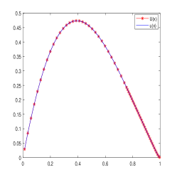
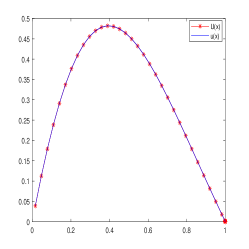
Figure 1: Numerical approximation of $u$: $\varepsilon=10^{-2}$ (left); $\varepsilon=10^{-4}$ (right).

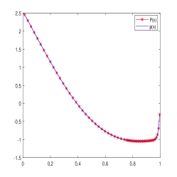
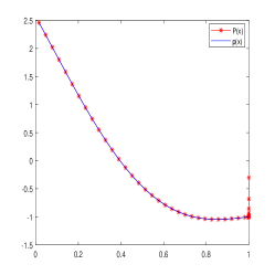
Figure 2: Numerical approximation of $p$: $\varepsilon=10^{-2}$ (left); $\varepsilon=10^{-4}$ (right).

Table 3: Energy-error and convergence rate for $\varepsilon=10^{-4}$.

		S-mesh		BS-mesh		B-mesh
	$N$	error	$r_{s}$-order	error	$r_{2}$-order	error	$r_{2}$-order
${{\cal P}^{0}}$	16	3.87e-01	-	3.87e-01	-	3.87e-01	-
	32	2.40e-01	1.02	2.40e-01	0.69	2.40e-01	0.69
	64	1.56e-01	0.84	1.56e-01	0.62	1.56e-01	0.62
	128	1.05e-01	0.73	1.05e-01	0.57	1.05e-01	0.57
	256	7.21e-02	0.67	7.21e-02	0.54	7.20e-02	0.54
	512	5.02e-02	0.63	5.02e-02	0.52	5.02e-02	0.52
${{\cal P}^{1}}$	16	2.57e-02	-	2.57e-02	-	2.56e-02	-
	32	8.71e-03	2.30	8.71e-03	1.56	8.69e-03	1.56
	64	3.01e-03	2.08	3.01e-03	1.53	3.00e-03	1.53
	128	1.05e-03	1.95	1.05e-03	1.52	1.05e-03	1.51
	256	3.70e-04	1.86	3.69e-04	1.51	3.68e-04	1.51
	512	1.30e-04	1.82	1.30e-04	1.51	1.30e-04	1.50
${{\cal P}^{2}}$	16	6.62e-04	-	6.51e-04	-	6.47e-04	-
	32	1.15e-04	3.72	1.08e-04	2.59	1.08e-04	2.58
	64	2.17e-05	3.26	1.85e-05	2.55	1.84e-05	2.55
	128	4.39e-06	2.96	3.20e-06	2.53	3.19e-06	2.53
	256	9.31e-07	2.77	5.60e-07	2.51	5.58e-07	2.52
	512	2.02e-07	2.66	9.85e-08	2.51	9.82e-08	2.51
${{\cal P}^{3}}$	16	3.16e-05	-	2.06e-05	-	2.04e-05	-
	32	5.37e-06	3.77	1.75e-06	3.56	1.73e-06	3.56
	64	8.99e-07	3.50	1.52e-07	3.53	1.50e-07	3.53
	128	1.37e-07	3.49	1.33e-08	3.51	1.31e-08	3.52
	256	1.94e-08	3.49	1.16e-09	3.52	1.16e-09	3.50
	512	2.60e-09	3.49	1.02e-10	3.51	1.02e-10	3.51

Table 4: Energy-error and convergence rate for $\varepsilon=10^{-8}$.

		S-mesh		BS-mesh		B-mesh
	$N$	error	$r_{2}$-order	error	$r_{2}$-order	error	$r_{2}$-order
${{\cal P}^{0}}$	16	3.87e-01	-	3.87e-01	-	3.87e-01	-
	32	2.40e-01	0.69	2.40e-01	0.69	2.40e-01	0.69
	64	1.56e-01	0.62	1.56e-01	0.62	1.56e-01	0.62
	128	1.05e-01	0.57	1.05e-01	0.57	1.05e-01	0.57
	256	7.21e-02	0.54	7.21e-02	0.54	7.20e-02	0.54
	512	5.02e-02	0.52	5.02e-02	0.52	5.02e-02	0.52
${{\cal P}^{1}}$	16	2.57e-02	-	2.57e-02	-	2.57e-02	-
	32	8.72e-03	1.56	8.72e-03	1.56	8.72e-03	1.56
	64	3.01e-03	1.53	3.01e-03	1.53	3.01e-03	1.53
	128	1.05e-03	1.52	1.05e-03	1.52	1.05e-03	1.52
	256	3.69e-04	1.51	3.69e-04	1.51	3.69e-04	1.51
	512	1.30e-04	1.51	1.30e-04	1.51	1.30e-04	1.51
${{\cal P}^{2}}$	16	6.52e-04	-	6.52e-04	-	6.52e-04	-
	32	1.09e-04	2.58	1.09e-04	2.58	1.08e-04	2.59
	64	1.85e-05	2.56	1.85e-05	2.56	1.85e-05	2.55
	128	3.21e-06	2.53	3.21e-06	2.53	3.21e-06	2.53
	256	5.62e-07	2.51	5.62e-07	2.51	5.62e-07	2.51
	512	9.89e-08	2.51	9.89e-08	2.51	9.89e-08	2.51
${{\cal P}^{3}}$	16	2.06e-05	-	2.06e-05	-	2.06e-05	-
	32	1.76e-06	3.55	1.76e-06	3.55	1.76e-06	3.55
	64	1.53e-07	3.52	1.52e-07	3.53	1.52e-07	3.53
	128	1.34e-08	3.51	1.33e-08	3.51	1.33e-08	3.51
	256	1.19e-09	3.49	1.17e-09	3.51	1.17e-09	3.51
	512	1.07e-10	3.48	1.03e-10	3.51	1.03e-10	3.51

Table 5: Energy-error and convergence rate for $\varepsilon=10^{-12}$.

		S-mesh		BS-mesh		B-mesh
	$N$	error	$r_{2}$-order	error	$r_{2}$-order	error	$r_{2}$-order
${{\cal P}^{0}}$	16	3.87e-01	-	3.87e-01	-	3.87e-01	-
	32	2.40e-01	0.69	2.40e-01	0.69	2.40e-01	0.69
	64	1.56e-01	0.62	1.56e-01	0.62	1.56e-01	0.62
	128	1.05e-01	0.57	1.05e-01	0.57	1.05e-01	0.57
	256	7.21e-02	0.54	7.21e-02	0.54	7.20e-02	0.54
	512	5.02e-02	0.52	5.02e-02	0.52	5.02e-02	0.52
${{\cal P}^{1}}$	16	2.57e-02	-	2.57e-02	-	2.57e-02	-
	32	8.72e-03	1.56	8.72e-03	1.56	8.72e-03	1.56
	64	3.01e-03	1.53	3.01e-03	1.53	3.01e-03	1.53
	128	1.05e-03	1.52	1.05e-03	1.52	1.05e-03	1.52
	256	3.69e-04	1.51	3.69e-04	1.51	3.69e-04	1.51
	512	1.30e-04	1.51	1.30e-04	1.51	1.30e-04	1.51
${{\cal P}^{2}}$	16	6.52e-04	-	6.52e-04	-	6.52e-04	-
	32	1.09e-04	2.58	1.09e-04	2.58	1.08e-04	2.59
	64	1.85e-05	2.56	1.85e-05	2.56	1.85e-05	2.55
	128	3.21e-06	2.53	3.21e-06	2.53	3.21e-06	2.53
	256	5.62e-07	2.51	5.62e-07	2.51	5.62e-07	2.51
	512	9.89e-08	2.51	9.89e-08	2.51	9.89e-08	2.51
${{\cal P}^{3}}$	16	2.06e-05	-	2.06e-05	-	2.06e-05	-
	32	1.76e-06	3.55	1.76e-06	3.55	1.76e-06	3.55
	64	1.53e-07	3.52	1.52e-07	3.53	1.52e-07	3.53
	128	1.34e-08	3.51	1.33e-08	3.51	1.33e-08	3.51
	256	1.19e-09	3.49	1.17e-09	3.51	1.17e-09	3.51
	512	1.07e-10	3.48	1.03e-10	3.51	1.03e-10	3.51

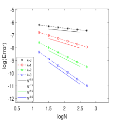
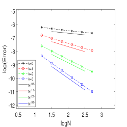
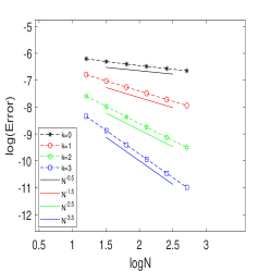
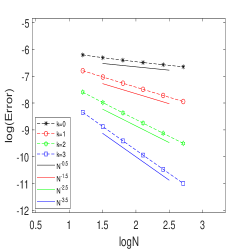
Figure 3: Energy-error: $\varepsilon=10^{-4}$ (top); $\varepsilon=10^{-8}$ (bottom); left: S mesh; middle: BS mesh; right: B mesh.

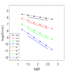
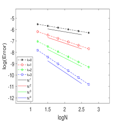
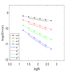
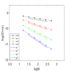
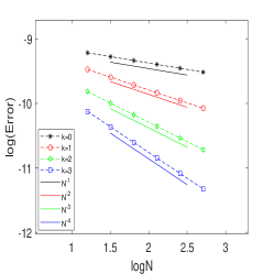
Figure 4: $L^{2}$-error $\|u-U\|$: $\varepsilon=10^{-4}$ (top); $\varepsilon=10^{-8}$ (bottom); left: S mesh; middle: BS mesh; right: B mesh.

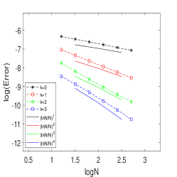
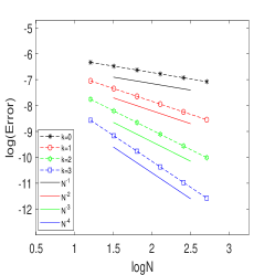
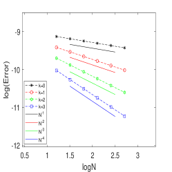
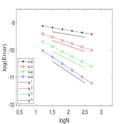
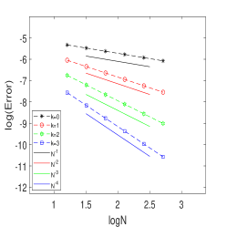
Figure 5: $L^{2}$-error $\|p-P\|$: $\varepsilon=10^{-4}$ (top); $\varepsilon=10^{-8}$ (bottom); left: S mesh; middle: BS mesh; right: B mesh.

5 Concluding remarks

In this study, we considered the local discontinuous Galerkin method on three typical layer-adapted meshes for a third-order singularly perturbed problem of convection-diffusion type. We obtained a quasi-optimal error estimate in the energy norm. The convergence rate is uniformly valid with respect to a small perturbation parameter. The theoretical findings provide insights into the discontinuous Galerkin method for higher-order singularly perturbed problems. Extension of such results to higher odd-order singularly perturbed problems and higher dimensional singularly perturbed problems constitute our future work.

Appendix

In this part, we provide a technical lemma used in the proof of our main result.

Lemma 4.

Suppose $(X,Y)\in\mathcal{V}_{N}^{2}$ satisfies

$$\langle Y,s\rangle_{I_{j}}+\varepsilon(\langle X,s^{\prime}\rangle_{I_{j}}-{\hat{X}}_{j}s_{j}^{-}+{\hat{X}}_{j-1}s_{j-1}^{+})=F_{j}(s)$$ (A.1)

in each element $I_{j}\in\Omega_{N}$ and for any test function $s\in\mathcal{V}_{N}$, where $F_{j}(s):\mathcal{V}_{N}\to R$ is a linear functional, and

$$\hat{X}_{j}=\begin{cases}X_{j}^{+},\hskip 20.00003ptj=0,1,\ldots,N-1,\\ 0,\hskip 30.00005ptj=N.\end{cases}$$

Then, the local estimate holds

$$\|Y\|_{I_{j}}\leq C\varepsilon\left(h_{j}^{-1}\|X\|_{I_{j}}+h_{j}^{-1/2}|[\![X]\!]_{j}|\right)+\frac{|{F_{j}}(Y)|}{\|Y\|_{I_{j}}}$$ (A.2)

for each element $I_{j}\in\Omega_{N}$, where $C>0$ is independent of $\varepsilon$ and $h_{j}$.

Proof. Take $s=Y$ into (A.1), use integration by parts, an inverse inequality and the Cauchy-Schwarz inequality to get

$$\|Y\|_{I_{j}}^{2} =\varepsilon(-\langle X,Y^{\prime}\rangle_{I_{j}}+X_{j}^{+}Y_{j}^{-}-X_{j-1}^{+}Y_{j-1}^{+})+F_{j}(Y)$$

$$=\varepsilon(\langle X^{\prime},Y\rangle_{I_{j}}+Y_{j}^{-}[\![X]\!]_{j})+F_{j}(Y)$$

$$\leq C\varepsilon(h_{j}^{-1}\|X\|_{I_{j}}\|Y\|_{I_{j}}+h_{j}^{-1/2}|[\![X]\!]_{j}|\|Y\|_{I_{j}})+|F_{j}(Y)|$$

for $j=1,2,\dots,N-1$. Hence,

$$\|Y\|_{I_{j}} \leq C\varepsilon(h_{j}^{-1}\|X\|_{I_{j}}+h_{j}^{-1/2}|[\![X]\!]_{j}|)+\frac{|F_{j}(Y)|}{\|Y\|_{I_{j}}}$$

hold for $j=1,2,\dots,N-1$. Analogously, one can obtain the conclusion for $j=N$ by noticing that $[\![X]\!]_{N}=-X_{N}^{-}$.

References

- [1] Yao Cheng, On the local discontinuous Galerkin method for singularly perturbed problem with two parameters, J. Comput. Appl. Math. 392 (2021), Paper No. 113485, 22.
- [2] Yao Cheng, Yanjie Mei, and Hans-Görg Roos, The local discontinuous Galerkin method on layer-adapted meshes for time-dependent singularly perturbed convection-diffusion problems, Comput. Math. Appl. 117 (2022), 245–256.
- [3] Yao Cheng, Li Yan, Xuesong Wang, and Yanhua Liu, Optimal maximum-norm estimate of the LDG method for singularly perturbed convection-diffusion problem, Appl. Math. Lett. 128 (2022), Paper No. 107947, 11.
- [4] Yao Cheng and Qiang Zhang, Local analysis of the local discontinuous Galerkin method with generalized alternating numerical flux for one-dimensional singularly perturbed problem, J. Sci. Comput. 72 (2017), no. 2, 792–819.
- [5] Philippe G. Ciarlet, The finite element method for elliptic problems, Studies in Mathematics and its Applications, Vol. 4, North-Holland Publishing Co., Amsterdam-New York-Oxford, 1978. MR 0520174
- [6] Bernardo Cockburn and Chi-Wang Shu, The local discontinuous Galerkin method for time-dependent convection-diffusion systems, SIAM J. Numer. Anal. 35 (1998), no. 6, 2440–2463.
- [7] F. A. Howes, The asymptotic solution of a class of third-order boundary value problems arising in the theory of thin film flows, SIAM J. Appl. Math. 43 (1983), no. 5, 993–1004.
- [8] , Nonlinear dispersive systems: theory and examples, Stud. Appl. Math. 69 (1983), no. 1, 75–97.
- [9] Torsten Linß, The necessity of Shishkin decompositions, Appl. Math. Lett. 14 (2001), no. 7, 891–896.
- [10] Torsten Linß, Layer-adapted meshes for reaction-convection-diffusion problems, Lecture Notes in Mathematics, vol. 1985, Springer-Verlag, Berlin, 2010.
- [11] Robert E. O’Malley, Introduction to singular perturbations, Applied mathematics and mechanics, vol. 89, New York : Academic Press, 1974.
- [12] Hans-Goerg Roos, Ljiljana Teofanov, and Zorica Uzelac, Uniformly convergent difference schemes for a singularly perturbed third order boundary value problem, Appl. Numer. Math. 96 (2015), 108–117.
- [13] Hans-Görg Roos, Martin Stynes, and Lutz Tobiska, Robust numerical methods for singularly perturbed differential equations, second ed., Springer Series in Computational Mathematics, vol. 24, Springer-Verlag, Berlin, 2008, Convection-diffusion-reaction and flow problems.
- [14] R. S. Temsah, Spectral methods for some singularly perturbed third order ordinary differential equations, Numer. Algorithms 47 (2008), no. 1, 63–80.
- [15] S. Valarmathi and N. Ramanujam, An asymptotic numerical method for singularly perturbed third-order ordinary differential equations of convection-diffusion type, Comput. Math. Appl. 44 (2002), no. 5-6, 693–710.
- [16] Ziqing Xie, Zuozheng Zhang, and Zhimin Zhang, A numerical study of uniform superconvergence of LDG method for solving singularly perturbed problems, J. Comput. Math. 27 (2009), no. 2-3, 280–298.
- [17] Helena Zarin, Hans-Görg Roos, and Ljiljana Teofanov, A continuous interior penalty finite element method for a third-order singularly perturbed boundary value problem, Comput. Appl. Math. 37 (2018), no. 1, 175–190.
- [18] Huiqing Zhu and Zhimin Zhang, Convergence analysis of the LDG method applied to singularly perturbed problems, Numer. Methods Partial Differential Equations 29 (2013), no. 2, 396–421.
- [19] , Uniform convergence of the LDG method for a singularly perturbed problem with the exponential boundary layer, Math. Comp. 83 (2014), no. 286, 635–663.