Designing Universal Causal Deep Learning Models: The Case of Infinite-Dimensional Dynamical Systems from Stochastic Analysis

Abstract

Causal operators (CO), such as various solution operators to stochastic differential equations, play a central role in contemporary stochastic analysis; however, there is still no canonical framework for designing Deep Learning (DL) models capable of approximating COs. This paper proposes a “geometry-aware” solution to this open problem by introducing a DL model-design framework that takes suitable infinite-dimensional linear metric spaces as inputs and returns a universal sequential DL model adapted to these linear geometries. We call these models Causal Neural Operators (CNOs). Our main result states that the models produced by our framework can uniformly approximate on compact sets and across arbitrarily finite-time horizons Hölder or smooth trace class operators, which causally map sequences between given linear metric spaces. Our analysis uncovers new quantitative relationships on the latent state-space dimension of CNOs which even have new implications for (classical) finite-dimensional Recurrent Neural Networks (RNNs). We find that a linear increase of the CNO’s (or RNN’s) latent parameter space’s dimension and of its width, and a logarithmic increase of its depth imply an exponential increase in the number of time steps for which its approximation remains valid. A direct consequence of our analysis shows that RNNs can approximate causal functions using exponentially fewer parameters than ReLU networks.

1 Introduction

Infinite-dimensional (non-linear) dynamical systems play a central role in several sciences, especially for disciplines driven by stochastic analytic modeling. However, despite this fact, the causal neural network approximation theory for most relevant dynamical systems in stochastic analysis remain largely misunderstood. Indeed, we currently only comprehend neural network approximations of Stochastic Differential Equations (SDEs) with deterministic coefficients (e.g., G2021FS ) and time-invariant random dynamical systems with the fading memory and echo state property/unique solution property (e.g., JaegerFMP ; Gonon2022NNs ). A significant problem is causal neural network approximation of solution operators to non-Markovian SDEs.
Moreover, the understanding of how sequential deep learning models work is still not fully developed, even in the classical finite-dimensional setting. For instance, the seemingly elementary empirical fact that a sequential DL model’s expressiveness increases when one utilizes a high-dimensional latent state space is understood qualitatively for general dynamical systems on Euclidean spaces (as in the reservoir computing literature (e.g., Lukas_StochInputReservoir )).

However, the quantitative understanding of the relationship between a sequential learning model’s state and its expressiveness remains an open problem. One notable exception to this fact is the approximation of linear state-space dynamical systems by a stylized class of Recurrent Neural Networks (RNNs, henceforth); see helmut2022metric ; LiJMLR2022 .

Our contribution.

Our paper provides a simple quantitative solution to a far reaching generalization of the above problem of constructing neural network approximation of infinite-dimensional (generalized) dynamical systems on “good” linear metric spaces. More precisely, we construct a neural network approximation of any function $f$ that “causally” and “regularly” maps sequences $(x_{t_{n}})_{n=-\infty}^{\infty}$ to sequences $(y_{t_{n}})_{n=-\infty}^{\infty}$, where each $x_{t_{n}}$ and every $y_{t_{n}}$ lives in a suitable linear metric space. In particular, we construct our causal neural network approximation framework on the following desiderata:

1. Predictions are causal, i.e., each $y_{t_{n}}$ is predicted independently of $(x_{t_{m}})_{m>n}$.

2. Each $y_{t_{n}}$ is predicted with a small neural network specialized at time $t_{n}$.

3. Only one of these specialized networks is stored in working memory at a time.

We first begin by describing our causal neural network model’s design. Subsequently, we will discuss our approximation theory’s implications in computational stochastic analysis.

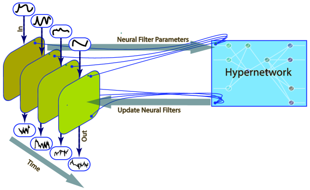
Figure 1: The Causal Neural Operator Model:
Summary: An efficient universal approximator of causal sequences of operators between well-behaved Fréchet spaces.
Overview: The model successively applies a “universal” neural filter (see Figure 2) on consecutive time-windows; the internal parameters of this neural filter are evolve according to a latent dynamical system on the neural filter’s parameter space; implemented by a deep ReLU network called a hypernetwork.

Our neural network model, which we call the Causal Neural Operator (CNO, henceforth) is illustrated in Figure 1 and works in the following way. At any given time $t_{n}$, it predicts an instance of the output time-series at that time $t_{n}$ using an immediate time-window from the input time-series (e.g., it predicts each $y_{t_{n}}$ using only $(x_{t_{i}})_{i=n-10}^{n}$). At each time $t_{n}$, this prediction is generated by a non-linear operator defined by a finitely parameterized neural network model, called a neural filter (the vertical black arrows in Figure 1). Our neural network model stores only one neural filter’s parameters in working memory at the current time by using an auxiliary ReLU neural network, called a hypernetwork in the machine learning literature (e.g., HDQICLR2017 ; VOHSG2020ICLR ), to generate the next neural filter specialized at $t_{n+1}$ using only the parameters of the current “active” neural filter specialized at time $t_{n}$ (the blue box in Figure 1). Thus, a dynamical system (i.e., the hypernetwork) on the neural filter’s parameter space interpolating between each neural filter’s parameters encodes our entire model.

The principal approximation-theoretic advantage of this approach lies in the fact that the hypernetwork is not designed to approximate anything, but rather, it only needs to memorize/interpolate a finite number of finite-dimensional (parameter) vectors. Since memorization (e.g., VershinynMemorization ; KDDWP2022 ) requires only a polynomial number of parameters, while approximation yarotsky2017error ; KP2022JMLR ; ZHS2022JMPA ; BehnooshAnastasisTMLR requires an exponential number of them, then, if memorization can be leveraged, the constructed neural network model is exponentially more efficient. Thus, this neural network design allows us to successfully encode all the parameters required to approximate long stretches of time $\{t_{0},\dots,t_{N}\}$ (for large $N$) with far fewer parameters (i.e., at the cost of $O(\log(N))$ additional layers in the hypernetwork). Thus, we successfully achieve desiderata (D1)–(D3) provided that each neural filter relies on only a small number of parameters. We show that this is the case whenever $f$ is “sufficiently smooth”; the rigorous formulation of all these outlined ideas are expressed in Lemma 5 and Theorem 3.2.

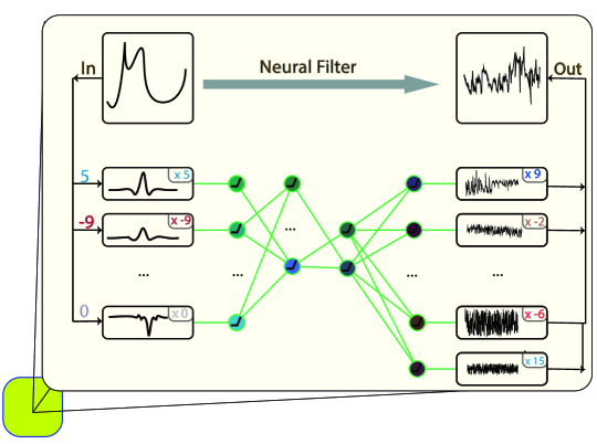
Figure 2: The Neural Filter
Summary: An efficient universal approximator between any well-behaved Fréchet spaces.
Overview: The neural filter first encodes inputs from a (possibly infinite-dimensional) linear space by approximate representing the input as coefficients of an sparse (Schauder) basis. These basis coefficients are then transformed by a deep ReLU network and the network’s outputs are decoded by into coefficients of a sparse basis representation of an element of the output linear space. Assembling the basis using the outputted coefficients produces the neural filter’s output.

Though we are focused on the approximation theoretic properties of our modeling framework, we have designed our CNO by considering practical considerations. Namely, we intentionally designed the CNO model so that, like transformer networks VawaniTransformers2017 , it can be trained non-recursively (via our federated training algorithm, see Algorithm 1 below). This design choice is motivated by the main reasons why the transformer network model (e.g., VawaniTransformers2017 ) has replaced residual (e.g., H2020CVPR ) and RNN (especially Long Short-Term Memory (LSTMs, henceforth) HochNeurCom1997 ) counterparts in practice (e.g., Hop1982NA ; Wi1986NATURE ); namely, not back-propagating through time during training. The reason is that omitting any recurrence relation between a model’s prediction in sequential prediction tasks, at-least during the model’s construction, has been empirically confirmed to yield more reliable and accurate models trained faster and without vanishing or exploding gradient problems; see, e.g., HochVanishing ; Pa2013ICML . Nevertheless, our model does ultimately reap the benefits of recursive models even if we construct it non-recursively, using our parallelizable training procedure.

The neural filter, illustrated in Figure 2, is a neural operator with quantitative universal approximation guarantees far beyond the Hilbert space setting. It works by first encoding infinite-dimensional problems into finite-dimensions problems, as the Fourier Neural Operator (FNO, henceforth) of LiICLR2019 , using a predetermined truncated Schauder basis. It then predicts outputs by passing the truncated basis coefficients through a feed-forward neural network with trainable (P)ReLU activation function. Finally, it reassembles them in the output space by interpreting that network’s outputs as the coefficients of a pre-specified Schauder basis or if both spaces are reproducing kernel Hilbert spaces then the first few basis functions can learned from data using principal component analysis, e.g. as with PCA–Net PCANET2023 . Similarly, instead complete a set of parameterized function (learned linearly independent) learned during training, as is implicitly the case with the DeepONet architecture DeepONet2021Nature ; which are universal when inputs and outputs belong to certain Sobolev Spaces in which the parameterized (neural network) functions are universal approximators hornik1990 .
Our “static” efficient approximation theorems provides quantitative approximation guarantees for several “neural operators” used in practice, especially in the numerical Partial Differential Equations (PDEs) (e.g., Kar2021PR ) and the inverse-problem literature (e.g., An2020IOP ; Bub2021IOP ; Al2021Neurips ; Bub2021ISIAMIS ; deHoop2020MSL ). Notable examples are the FNO (see Kov2021JMLR for a qualitative universal result and quantitative guarantees for approximation of the Darcy flow and incompressible Navier-Stokes PDEs (Kov2021JMLR, , Theorem 26 and 32), respectively), the wavelet neural operator recently introduced in the numerical PDE literature (Tr2022ArXiV ), and several other neural operators who now have quantitative universal approximation guarantees thanks to our “static” universal approximation result, when the target map is assumed to be sufficiently regular (for a more precise statement refer to Definition 5 and 6). The same argument is valid also for the general qualitative theorems of Sithcompact1996 ; LucaUATPaperI .
We now describe more in detail the different areas in which the present paper contributes.

Our contribution in the Approximation Theory of Neural Operators.

Our results provide the first set of quantitative approximation guarantees for generalized dynamical systems evolving on general infinite-dimensional spaces. By refining the memorizing hypernetwork argument of AKP2022WP , together with our general solution to the static universal approximation problem, in the class of Hölder functions, we are able to confirm a well-known folklore approximation of dynamical systems literature. Namely, that increasing a sequential neural operator’s latent space’s dimension by a positive integer $Q$ and our neural network’s depth by $\tilde{\mathcal{O}}(T^{-Q}\log(T^{-Q}))$ and width by $\tilde{\mathcal{O}}(QT^{-Q})$ implies that we may approximate $\mathcal{O}(T)$ more time-steps in the future with the same prescribed approximation error.

To the best of our knowledge, our dynamic result is the only quantitative universal approximation theorem guaranteeing that a recurrent neural network model can approximate any suitably regular infinite-dimensional non-linear dynamical systems. Likewise, our static result is to the best of our knowledge the only general infinite-dimensional guarantee showing that a neural operator enjoys favourable approximation rates when the target map is smooth enough.

Our contribution in the Approximation Theory of RNNs

In the finite-dimensional context, CNOs become strict sub-structures of full RNNs, where the internal parameters are updated/generated via an auxiliary hypernetwork. Noticing this structural inclusion, our results rigorously justify the folklore that RNNs can approximate causal maps strictly more efficiently than feedforward neural network (FFNN, henceforth), see Section 5.

Technical contributions:

Our results apply to sequences of non-linear operators between any “good linear” metric spaces. By “good linear” metric space we mean any Fréchet space admitting Schauder basis. This includes many natural examples (e.g., the sequence space $\mathbb{R}^{\mathbb{N}}$ with its usual metric) outside the scope of the Banach, Hilbert spaces carrying Schauder basises and Euclidean settings; which are completely subsumed by our assumptions. In other words, we treat the most general tractable linear setting where one can hope to obtain quantitative universal approximation theorems.

Organization of our paper

This research project answers theoretical deep learning questions by combining tools from approximation theory, functional analysis, and stochastic analysis. Therefore, we provide a concise exposition of each of the relevant tools from these areas in our “preliminaries” Section 2.
Section 3 contains our quantitative universal approximation theorems. In the static case, we derive expression rates for the static component of our model, namely the neural filters, which depend on the regularity of the target operator being approximated; from Hölder trace-class to smooth trace-class and on the usual quantities. Our main approximation theorem in the dynamic case additionally encodes the target causal map’s memory decay rate.

Section 4 applies our main results to derive approximation guarantees for the solution operators of a broad range of SDEs with stochastic coefficients, possibly having jumps (“stochastic discontinuities”) at times on a pre-specified time-grid and with initial random noise. Section 5, examines the implication of our approximation rates for RNNs, in the finite-dimensional setting, where we find that RNNs are striclty more efficient than FFNN when approximating causal maps. Section 6 concludes. Finally, Appendix A contains any background material required in the derivations of our main results whose derivations are relegated to Appendix B.

1.1 Notation

For the sake of the reader, we collect and define here the notations we will use in the rest of the paper, or we indicate the exact point where the first appearance of a symbol occurs:

1. $\mathbb{N}_{+}$ : it is the set of natural numbers strictly greater than zero, i.e. $1,2,3,\cdots$. On the other hand, we use $\mathbb{N}$ to denote the positive integers, and $\mathbb{Z}$ to denote the integers.

2. $[[N]]$ : it denotes the set of natural numbers between $1$ and $N$, $N\in\mathbb{N}_{+}$, i.e. $[[N]]=\{1,\ldots,N\}$.

3. Given a topological vector space $(F,\tau)$, $F^{\prime}$ will denote its topological dual, namely the space of continuous linear forms on $F$.

4. Given two topological vector spaces $(E,\sigma)$ and $(F,\tau)$, $L(E,F)$ denotes the space of continuous linear operators from $E$ into $F$; if $E=F$, then we will write $L(E)=L(E,E)$.

5. Given a Fréchet space $F$, we use $\langle\cdot,\cdot\rangle$ to denote the canonical pairing of $F$ with its topological dual $F^{\prime}$,

6. We denote the open ball of radius $r>0$ about a point $x$ in a metric space $(X,d)$ by $\operatorname{Ball}_{(X,d)}(x,r)\stackrel{{\scriptstyle\mbox{\tiny def.}}}{{=}}\{u\in X:\,d(x,u)<r\}$,

7. We denote the closure of a set $A$ in a metric space $(X,d)$ by $\overline{A}$.

8. $\mathcal{P},p_{k}$: 2.1

9. $\Phi$: (2)

10. $\beta_{k}^{F}$ with $F$= Fréchet space: (7)

11. $d_{F:n}$ with $F$= Fréchet space: (8)

12. $[d],P([d])$: 2.3

13. $P_{F:n},I_{F:n}$ with $F$= Fréchet space: (12) and (13)

14. $C_{tr}^{k,\lambda}(K,B)$ and $C_{\alpha,tr}^{\lambda}(K,B)$: 5 and 6

15. $\psi_{n}$ and $\varphi_{n}$: (15) (16)

16. The canonical projection onto the $n^{th}$ coordinate of an $x\in\prod_{n\in\mathbb{Z}}\,\mathcal{X}_{n}$ is denoted by $x_{n}$; where each $\mathcal{X}_{n}$ is an arbitrary non-empty set.
    In particular, if $f:A\rightarrow\prod_{n\in\mathbb{Z}}\,\mathcal{X}_{n}$, with $A$ an arbitrary non-empty set, then $f(x)_{n}$ denotes the projection of $f(x)\in\prod_{n\in\mathbb{Z}}\,\mathcal{X}_{n}$ onto the $n^{th}$ coordinate,

17. $\mathcal{NF}^{\text{(P)ReLU}}_{[n]}$: The set of neural filters from $B$ to $E$,

18. $V$: the “special function”, defined as the inverse of the map $u\mapsto u^{4}\,\log_{3}(u+2)$ on $[0,\infty)$.

2 Preliminaries

In this section, we remind some preparatory material for the derivations of the main results of this paper. Finally, we remark that the notation in each of the subsequent subsections is self-contained and it is the one used on the cited paper: it will be up to the reader to contextualize it in the next sections.

2.1 Fréchet spaces

The main references for this subsection are the following ones: H1982AMS , Part I; C2019 Chapter IV; S1971 , Chapter III and the working paper of BONET2020WP ; all the vector spaces we will deal with will be vector spaces over $\mathbb{R}$. Before defining a Fréchet space, we remind that a locally convex topological vector space, say $(F,\tau)$, is a topological vector space whose topology $\tau$ arises from a collection of seminorms $\mathcal{P}$. When clear from the context, we will write $F$ instead of $(F,\tau)$. The topology is Hausdorff if and only if for every $x\in F$ with $x\neq 0$ there exists a $p\in\mathcal{P}$ such that $p(x)>0$. On the other hand, the topology is metrizable if and only if it may be induced by a countable collection $\mathcal{P}=\{p_{k}\}_{k\in\mathbb{N}_{+}}$ of seminorms, which we may assume to be increasing, namely $p_{k}(\cdot)\leq p_{k+1}(\cdot),k\in\mathbb{N}_{+}$.

Definition 1 (Fréchet space)

A Fréchet space $F$ is a complete metrizable locally convex topological vector space.

Evidently, every Banach space $(F,\|\cdot\|_{F})$ is a Fréchet space; in this case, simply $\mathcal{P}=\{\|\cdot\|_{F}\}$.
A canonical choice for the metric $d_{F}$ on a Fréchet space $F$ (that generates the pre-existing topology) is given by:

$$d_{F}(x,y)\stackrel{{\scriptstyle\mbox{\tiny def.}}}{{=}}\sum_{k=1}^{\infty}2^{-k}\,\Phi(p_{k}(x-y)),\quad x,y\in F,$$ (1)

where

$$\Phi(t)\stackrel{{\scriptstyle\mbox{\tiny def.}}}{{=}}\frac{t}{1+t},\,\,\,t\geq 0.$$ (2)

We now remind the concept of directional derivative of a function between two Frećhet spaces. This notion of differentiation is significantly weaker than the concept of the derivative of a function between two Banach spaces. Nevertheless, it is the weakest notion of differentiation for which many of the familiar theorems from calculus hold. In particular, the chain rule is true (cfr. H1982AMS ). Let $F$ and $G$ be Fréchet spaces, $U$ an open subset of $F$, and $P:U\subseteq F\rightarrow G$ a continuous map.

Definition 2 (Directional Derivative)

The derivative of $P$ at the point $x\in U$ in the direction $h\in F$ is defined by:

$$DP(x)h=\lim_{t\rightarrow 0}\frac{P(x+th)-P(x)}{t}.$$ (3)

In particular, $P$ is said to be differentiable at $x$ in the direction $h$ if the previous limit exists. $P$ is said to be $C^{1}$ on $U$ if the limit in Equation(3) exists for all $x\in U$ and all $h\in F$, and $DP:(U\subseteq F)\times F\rightarrow G$ is continuous (jointly as a function on a subset of the product).

As anticipated, the Definition 2 of a $C^{1}$ map disagrees with the usual definition for a Banach space in the sense that the derivative will be the same map, but the continuity requirement is weaker. The previous definition can be generalized and applied to higher-order derivatives. For instance, if $P:U\subseteq F\rightarrow G$, then:

$$D^{2}P(x)\{h,k\}=\lim_{t\rightarrow 0}\frac{DP(x+tk)h-DP(x)h}{t}.$$ (4)

Analogously, $P$ is said to be $C^{2}$ on $U$ if $DP$ is $C^{1}$, which happens if and only if $D^{2}P$ exists and is continuous. If $P:U\subset F\to G$ we require $D^{2}P$ to be continuous jointly as a function on the product space

$$D^{2}P:(U\subseteq F)\times F\times F\to G.$$

Similarly, the $k$-th derivative $D^{k}P(x)\{h_{1},h_{2},\ldots,h_{k}\}$ will be regarded as a map

$$D^{k}P:(U\subseteq F)\times F\times\ldots\times F\rightarrow G.$$ (5)

$P$ is of class $C^{k}$ on $U$ if $D^{k}P$ exists and is continuous (jointly as a function on the product space).

Remark 1

We will say that $P$ is $C^{k}$-Dir if $P$ satisfies the previous definition.

Next, we introduce the concept of Schauder basis (MV1992 ). Let $F$ be a Fréchet space. A sequence $(f_{k})_{k\in\mathbb{N}_{+}}\subset F$ is called a Schauder basis if every $x\in F$ has a unique representation

$$x=\sum_{k=1}^{\infty}x_{k}f_{k},$$ (6)

where the series converges in $F$ (in the ordinary sense). It is immediate to see from the definition that the maps

$$F\ni x\stackrel{{\scriptstyle\beta_{k}^{F}}}{{\longmapsto}}x_{k},\quad k\in\mathbb{N}_{+}$$ (7)

are continuous linear functionals. We remind that if a Fréchet space admits a Schauder basis, it is separable. However, the converse does not hold in general; whether every separable Banach space has a basis appeared in 1931 for the first time in the Polish edition of Banach’s book (B1932 ) and was solved in the negative by Enflo (E1973AM ).
We now state and prove the following auxiliary lemma.

Lemma 1

Let F be a separable Fréchet space admitting a Schauder basis $(f_{k})_{k\in\mathbb{N}_{+}}$ and $d_{F}$ a metric on F compatible with the pre-existing topology (see Equation (1)). Fix $n\in\mathbb{N_{+}}$ and define on $\mathbb{R}^{n}$ the following metric:

$$d_{F:n}(x,y)\stackrel{{\scriptstyle\mbox{\tiny def.}}}{{=}}d_{F}\biggl{(}\sum_{k=1}^{n}x_{k}f_{k},\sum_{k=1}^{n}y_{k}f_{k}\biggr{)},\quad x,y\in\mathbb{R}^{n}.$$ (8)

Then, the topology induced on $\mathbb{R}^{n}$ by this metric is the standard one.

Proof

First, notice that $d_{F:n}$ is a metric on $F$. This follows directly from the fact that $d_{F}$ is a metric. Now, let $x^{(J)}\stackrel{{\scriptstyle\mbox{\tiny def.}}}{{=}}(x_{1}^{(J)},\ldots,x_{n}^{(J)}),\,J\in\mathbb{N}$ and $x\stackrel{{\scriptstyle\mbox{\tiny def.}}}{{=}}(x_{1},\ldots,x_{n})$ such that

$$x^{(J)}\underset{J\rightarrow\infty}{\overset{d_{F:n}}{\longrightarrow}}x.$$

This means in particular that

$$d_{F}\left(\sum_{k=1}^{n}x_{k}^{(J)}f_{k},\sum_{k=1}^{n}x_{k}f_{k}\right)\underset{J\rightarrow\infty}{\longrightarrow}0,\,\,\,i.e.,\,\,\,\sum_{k=1}^{n}x_{k}^{(J)}f_{k}\underset{J\rightarrow\infty}{\overset{F}{\longrightarrow}}\sum_{k=1}^{n}x_{k}f_{k}.$$

Now, let $(\beta_{k}^{F})_{k\leq n}$ be the unique sequence in the topological dual of $F$, say $F^{{}^{\prime}}$, such that each $f\in F$ has the following representation $f=\sum_{k=1}^{\infty}\langle\beta_{k}^{F},f\rangle f_{k}$. Because $(\beta_{k}^{F})_{k\leq n}$ are continuous and linear, we clearly get that $x_{k}^{(J)}\underset{J\rightarrow\infty}{\longrightarrow}x_{k}$ for each $k\in[[n]]$. This implies that

$$\left[\sum_{k=1}^{n}|x_{k}^{(J)}-x_{k}|^{2}\right]^{1/2}\underset{J\rightarrow\infty}{\longrightarrow}0,\,\,\,i.e.\,\,\,x^{(J)}\underset{J\rightarrow\infty}{\overset{\|\,\cdot\,\|_{2}}{\longrightarrow}}x.$$

Vice-versa, let $x^{(J)}\stackrel{{\scriptstyle\mbox{\tiny def.}}}{{=}}(x_{1}^{(J)},\ldots,x_{n}^{(J)})$ and $x\stackrel{{\scriptstyle\mbox{\tiny def.}}}{{=}}(x_{1},\ldots,x_{n})$ such that $x^{(J)}\underset{J\rightarrow\infty}{\overset{\|\cdot\|_{2}}{\longrightarrow}}x$. This implies that $\sum_{k=1}^{n}|x_{k}^{(J)}-x_{k}|\underset{J\rightarrow\infty}{\longrightarrow}0$. We pick an arbitrary continuous seminorm $p\in\mathcal{P}$. It holds for all $(t_{1},\ldots,t_{n})\in\mathbb{R}^{n}$ that

$$\begin{split}p\left(\sum_{k=1}^{n}t_{k}f_{k}\right)\leq\sum_{k=1}^{n}|t_{k}|p(f_{k})\leq\max_{k=1,\ldots,n}p(f_{k})\sum_{k=1}^{n}|t_{k}|.\end{split}$$

This shows that

$$p\left(\sum_{k=1}^{n}x_{k}^{(J)}f_{k}-\sum_{k=1}^{n}x_{k}f_{k}\right)\underset{J\rightarrow\infty}{\longrightarrow}0$$

for all $p\in\mathcal{P}$. This means in particular that

$$d_{F}\left(\sum_{k=1}^{n}x_{k}^{(J)}f_{k},\sum_{k=1}^{n}x_{k}f_{k}\right)\underset{J\rightarrow\infty}{\longrightarrow}0,\,\,\,i.e.,\,\,\,d_{F:n}(x^{(J)},x)\underset{J\rightarrow\infty}{\rightarrow}0.$$

Since the metric spaces $(\mathbb{R}^{n},d_{F:n})$ and $(\mathbb{R}^{n},\|\cdot\|_{2})$ enjoy the same converging sequences, the topology must be the same.

2.2 Generalized inverses

EH2013MMOR wrote a thorough paper about generalized inverses and their properties. Analogously to EH2013MMOR , we understand increasing in the weak sense, that is, $T\,:\,\mathbb{R}\rightarrow\mathbb{R}$ is increasing if $T(x)\leq T(y)$ for all $x<y$. Also, we remind the notion of an inverse for such functions.

Definition 3 (Generalized Inverse)

For an increasing function $T\,:\,\mathbb{R}\rightarrow\mathbb{R}$ with $T(-\infty)\stackrel{{\scriptstyle\mbox{\tiny def.}}}{{=}}\lim_{x\downarrow-\infty}T(x)$ and $T(\infty)\stackrel{{\scriptstyle\mbox{\tiny def.}}}{{=}}\lim_{x\uparrow\infty}T(x)$, the generalized inverse $T^{-}\,:\,\mathbb{R}\rightarrow\bar{\mathbb{R}}=[-\infty,\infty]$ of $T$ is defined by

$$T^{-}(y)\stackrel{{\scriptstyle\mbox{\tiny def.}}}{{=}}\inf\{x\in\mathbb{R}\,:\,T(x)\geq y\},\quad y\in\mathbb{R},$$

with the convention that $\inf\,\varnothing=\infty$.

To keep our manuscript self-contained, we list some properties of generalized inverses which can be found in (EH2013MMOR , cfr. Proposition 1). We denote the range of a map $T:\mathbb{R}\rightarrow\mathbb{R}$ by $\operatorname{ran}\,T\stackrel{{\scriptstyle\mbox{\tiny def.}}}{{=}}\{T(x):\,x\in\mathbb{R}\}$.

Proposition 1 (Properties of Generalized Inverses)

Let $T$ be as in Definition 3 and let $x,y\in\mathbb{R}$. Then,

1. $T^{-}(y)=-\infty$ if and only if $T(x)\geq y$ for all $x\in\mathbb{R}$. Similarly, $T^{-}(y)=\infty$ if and only if $T(x)<y$ for all $x\in\mathbb{R}$.

2. $T^{-}$ is increasing. If $T^{-}(y)\in(-\infty,\infty)$, $T^{-}$ is left-continuous at $y$ and admits a limit from the right at $y$.

3. $T^{-}(T(x))\leq x$. If $T$ is strictly increasing, $T^{-}(T(x))=x$.

4. Let $T$ be right-continuous. Then $T^{-}(y)<\infty$ implies $T(T^{-}(y))\geq y$. Furthermore, $y\in\operatorname{ran}\,T\bigcup\{\inf\,\operatorname{ran}\,T,\sup\,\operatorname{ran}\,T\}$ implies $T(T^{-}(y))=y$. Moreover, if $y<\inf\operatorname{ran}\,T$ then $T(T^{-}(y))>y$ and if $y>\sup\operatorname{ran}\,T$ then $T(T^{-}(y))<y$.

2.3 Feedforward Neural Networks with ReLU and PReLU activation functions

We give the definition of feed-forward neural networks with ReLU activation function (ReLU FFNNs, henceforth) and with a trainable Parametric ReLU activation function (PReLU FFNNs, henceforth). Interestingly, Proposition 1 in yarotsky2017error shows that using a ReLU activation function is not much different from using a PReLU activation function, in the sense that it is possible to replace a ReLU FFNN with a PReLU FFNN while only increasing the number of units and weights by constant factors. However, the main advantage of using a PReLU FFNN with respect to a ReLU FFNN is that the former can synchronize the depth of several functions realized by ReLU FFNNs, a fact that will be extremely important in the derivation of Theorem 3.2. In particular, a PReLU activation function is any map $\sigma\,:\,\mathbb{R}\times\mathbb{R}\rightarrow\mathbb{R}$, $(\alpha,x)\rightarrow\sigma_{\alpha}(x)\stackrel{{\scriptstyle\mbox{\tiny def.}}}{{=}}\max\{x,\alpha x\}$; the parameter $\alpha$ is called slope. Notice that for $\alpha=0$ one obtains the ReLU activation function. As it is customary in the literature, in what follows we will often be applying the (P)ReLU activation function component-wise. More precisely, for any $\alpha\in\mathbb{R}$ and an $x\in\mathbb{R}^{N}$, $N\in\mathbb{N}_{+}$, we have

$$\sigma_{\alpha}\mathbin{\vbox{\hbox{\scalebox{0.77}{$\bullet$}}}}x\stackrel{{\scriptstyle\mbox{\tiny def.}}}{{=}}(\sigma_{\alpha}(x_{i}))_{i=1}^{N}.$$ (9)

Fix $J\in\mathbb{N}_{+}$ and a multi-index $[d]\stackrel{{\scriptstyle\mbox{\tiny def.}}}{{=}}(d_{0},\ldots,d_{J})$, and let $P([d])\stackrel{{\scriptstyle\mbox{\tiny def.}}}{{=}}J+\sum_{j=0}^{J-1}d_{j}(d_{j+1}+1)+d_{J}$. Weights, biases, and slopes are identified in a unique parameter $\theta\in\mathbb{R}^{P([d])}$ with

$$\mathbb{R}^{P([d])}\,\reflectbox{$\in$}\,\theta\iff((A^{(j)},b^{(j)},{\color[rgb]{0,0,0}{\alpha^{(j)}}})_{j=0}^{J-1}),c),\quad(A^{(j)},b^{(j)},{\color[rgb]{0,0,0}{\alpha^{(j)}}})\in\mathbb{R}^{d_{j+1}\times d_{j}}\times\mathbb{R}^{d_{j}}{\color[rgb]{0,0,0}{\times\mathbb{R}}},\,\,c\in\mathbb{R}^{d_{J}}.$$ (10)

With the previous identification, the recursive representation function of a $[d]$-dimensional deep feed-forward network is given by

$$\begin{split}\mathbb{R}^{P([d])}\times\mathbb{R}^{d_{0}}&\reflectbox{$\in$}(\theta,x)\rightarrow\hat{f}_{\theta}(x)\stackrel{{\scriptstyle\mbox{\tiny def.}}}{{=}}x^{(J)}+c,\\ x^{(j+1)}&\stackrel{{\scriptstyle\mbox{\tiny def.}}}{{=}}A^{(j)}\sigma_{{\color[rgb]{0,0,0}{\alpha^{(j)}}}}\mathbin{\vbox{\hbox{\scalebox{0.75}{$\bullet$}}}}(x^{(j)}+b^{(j)})\quad\text{for\,\,}j=0,\ldots,J-1,\\ x^{(0)}&\stackrel{{\scriptstyle\mbox{\tiny def.}}}{{=}}{\color[rgb]{0,0,0}{A^{(0)}}}x.\end{split}$$ (11)

We will refer to $J$ as $\hat{f}_{\theta}$’s depth. We will denote by $\mathcal{N}\mathcal{N}^{\operatorname{(P)ReLU}}_{[d]}$ a deep ReLU FFNN with complexity $[d]$.

3 Main Results

3.1 Static Case: Efficient Universal Approximation

We begin by treating the “static case” wherein we show that CNO’s neural filters, illustrated in Figure 3, are universal approximators of (non-linear) Hölder class operators between “good” linear spaces. We note that the application of the CNO only requires us to customize its neural filters to the relevant input and outputs’ geometries.

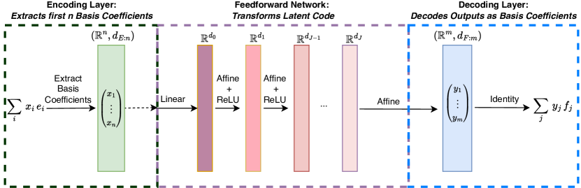
Figure 3: Illustration of our “static” operator network in Definition 7. The network is works in three phases. 1) First inputs are encoded as finite-dimensional Euclidean data by mapping them to their truncated (Schauder) basis coefficients in the input space $E$. 2) Next these coefficients are transformed by a ReLU FFNN. 3) The outputs of ReLU FFNN’s output are interpreted as coefficients for a truncated (Schauder) basis in the output space $F$.

We first fix our working setting for this section

1. Let $N,M\in\mathbb{N}_{+}\cup\{\infty\}$. Let $E$ and $B$ be two separable Fréchet spaces admitting Schauder bases $(e_{h})_{h\leq N}$ and $(b_{h})_{h\leq M}$. Let $E^{\prime}$ and $B^{\prime}$ be the topological dual of $E$ and $B$ respectively. Let $(\beta_{h}^{E})_{h\leq N}$ (resp. $(\beta_{h}^{B})_{h\leq M}$) be the unique sequence in $E^{\prime}$ (resp. $B^{\prime}$) such that each $e\in E$ (resp. each $b\in B$) has the following representation

   $$e=\sum_{h=1}^{N}\langle\beta_{h}^{E},e\rangle e_{h},\quad(resp.\,\,b=\sum_{h=1}^{M}\langle\beta_{h}^{B},b\rangle b_{h}),$$

   where $\langle\cdot\,,\,\cdot\rangle$ is the canonical pairing between $E^{{}^{\prime}}$ and $E$ (resp. between $B^{{}^{\prime}}$ and $B$). For each $n\in\mathbb{N}_{+}$, we denote by $P_{E:n}\,:\,(E,d_{E})\rightarrow(\mathbb{R}^{n},d_{E:n})$ the function defined as

   $$P_{E:n}:(E,d_{E})\rightarrow(\mathbb{R}^{n},d_{E:n}),\quad e\rightarrow(\langle\beta_{1}^{E},e\rangle,\langle\beta_{2}^{E},e\rangle,\ldots,\langle\beta_{n}^{E},e\rangle)^{T},$$ (12)

   where $d_{E:n}$ is the metric defined in Lemma 1. Moreover, $I_{E:n}\,:\,(\mathbb{R}^{n},d_{E:n})\rightarrow(E,d_{E})$ is the function defined as

   $$I_{E:n}\,:\,(\mathbb{R}^{n},d_{E:n})\rightarrow(E,d_{E}),\quad\beta\rightarrow\sum_{h=1}^{n}\beta_{h}e_{h}.$$ (13)

   Analogous definitions hold for $P_{B:n}$ and $I_{B:n}$.

Before proceeding, we make the following trivial, yet useful remark

Remark 2

Let $F$ be a separable Fréchet space – which can be either $E$ or $B$. Then, the maps $I_{F:n}$ and $P_{F:n}$ are continuous when $\mathbb{R}^{n}$ is endowed with the Euclidean topology. Therefore, they remain continuous when $\mathbb{R}^{n}$ is now endowed with the metric $d_{F:n}$, because the induced topology coincides with the Euclidean one; see Lemma 1.

In order to state our first approximation result, we introduce the notion of $C^{k}$-stability, $k\in\mathbb{N}$, of a non-linear operator mapping from a Fréchet space $E$ to a Fréchet space $B$.

Definition 4 ($C^{k}$-Stability)

Let $E$ and $B$ be two Fréchet spaces. A (non-linear) operator $f:E\rightarrow B$ is called $C^{k}$-stable if for every $m,n\in\mathbb{N}$, and every pair of continuous and linear maps $\tilde{I}:(\mathbb{R}^{n},\|\cdot\|_{2})\rightarrow(E,d_{E})$ and $\tilde{P}:(B,d_{B})\rightarrow(\mathbb{R}^{m},\|\cdot\|_{2})$ the following composition

$$\tilde{P}\circ f\circ\tilde{I}:\mathbb{R}^{n}\rightarrow\mathbb{R}^{m},$$ (14)

is of class $C^{k}$ in the usual sense.

We now state and prove the following lemma.

Lemma 2

Let $E$ and $B$ be two Fréchet spaces. Let $f:E\rightarrow B$ be a (non-linear) operator between these two spaces which is $C^{k}$-$Dir.$ (see Subsection 2.1, below Equation (5)). Then, $f$ is $C^{k}$ stable as in Definition 4.

Proof

See Appendix B, Subsection B.1

The restriction of any $C^{k}$-stable (non-linear) operator $f:E\rightarrow B$ between two Fréchet spaces $E$ and $B$ to any non-empty compact subset $K\subseteq E$ extends to a $C^{k}$-stable (non-linear) operator defined on all $E$, namely the function $f$ itself. However, because our approximation theorems will hold for a pair $(f,K)$ of a (non-linear) operator $f:E\rightarrow B$ and compact set $K$, then $f$ does not need to be smooth on $K$ but only indistinguishable from a smooth operator on $K$. That is, our main results focus on non-linear operators belonging to the following trace class.

Definition 5 (Trace Class $C^{k,\lambda}_{\operatorname{tr}}(K,B)$)

Let $E$ and $B$ be two Fréchet spaces and let $\lambda>0$ be a constant. Let $K\subseteq E$ be a non-empty compact set. We say that a (non-linear and possibly discontinuous) operator $f:E\rightarrow B$ belongs to the trace class $C^{k,\lambda}_{\operatorname{tr}}(K,B)$ if there exists a $\lambda$-Lipschitz $C^{k}$-stable (non-linear) operator $F:E\rightarrow B$ satisfying

$$F(x)=f(x)$$

for every $x\in K$.

The following Example 1, pictorially represented in Figure 4, highlights our main interest in trace class maps. Precisely, these maps can be globally poorly behaved, even discontinuous, but indistinguishable from smooth functions “locally” (i.e. on a particular compact subset of the input space $E$).

(a)

(b)

Figure 4: Pictorial representation of the fact that the indicator function of the interval $[0,1]$ belongs to $C^{k,\lambda}_{\operatorname{tr}}([0,1],\mathbb{R})$ for all $k\in\mathbb{N}$ and $\lambda>0$ ; see Example 1.

Example 1 (The indicator of the unit interval is in $C^{k,\lambda}_{\operatorname{tr}}(K,B)$)

Let $E=B=(\mathbb{R},|\cdot|)$, $K=[0,1]\cup[2,3]$, and $f=I_{[0,1]}$, i.e. the indicator function of the interval $[0,1]$. Then, by means of a bump function, we immediately see that for every $k\in\mathbb{N}$ and $\lambda>0$, $f\in C^{k,\lambda}_{\operatorname{tr}}(K,B)$.

At this point, some remarks are in order. In general, the problem of identifying when a map belongs to $C^{k,\lambda}_{\operatorname{tr}}(K,B)$ is a well-studied and independent area of research dating back to the beginning of the previous century (e.g., W1992 ). Nonetheless, by virtue of Lemma 2 a full characterization of the pairs of functions and sets $(f,K)$ that belongs to $C^{k,\lambda}_{\operatorname{tr}}(K,B)$ in the special case that $E$ and $B$ are Euclidean spaces has been derived only (relatively) recently in a series of articles starting with F2005AOM . The interested reader may consult BRUE2021JFA where the $C^{1,\lambda}_{\operatorname{tr}}(K,B)$ case is treated in the case that $B$ is Banach and $K$ is finite-dimensional (in a suitable metric-theoretic sense), for some $\lambda>0$ depending on $K$ and on $f$. The case where $K$ is a subset of a separable Hilbert space is explicitly solved in Azagra2018JFA .

Moreover, we provide results for the following trace class.

Definition 6 (Trace Class $C_{\alpha,\operatorname{tr}}^{\lambda}(K,B)$)

Let $E$ and $B$ be two Fréchet spaces, $\alpha\in(0,1]$ and $\lambda>0$ be two constants. Let $K\subseteq E$ be a non-empty compact set. We say that a (non-linear and possibly discontinuous) operator $f:E\rightarrow B$ belongs to the trace class $C_{\alpha,\text{tr}}^{\lambda}(K,B)$ if there exists an Hölder continuous (non-linear) operator $F:E\rightarrow B$ of order $\alpha$ and constant $\lambda$ satisfying

$$F(x)=f(x)$$

for every $x\in K$.

Functions with Hölder extensions are also actively studied. For example, (Lindenstrauss2000AMS, , Theorem 1.12) guarantees any Lipschitz function defined on a closed subset of a separable Hilbert space with values in a separable Hilbert space can be extended with the same Lipschitz constant. However, in general, the existence of Hölder extensions between Fréchet spaces, as well as quantitative estimates on the extension’s Hölder constant, can be subtle Naor2001Mathematika .

We state now our first main quantitative “efficient” approximation theorem; see Theorem 3.1. In order not to burden the statement of the theorem, we give here some definitions. First, for any $n\in\mathbb{N}_{+}$, we will use $\psi_{n}$ and $\varphi_{n}$ to denote the following two set-theoretic maps:

$$\psi_{n}\,:\,(\mathbb{R}^{n},d_{E:n})\longrightarrow(\mathbb{R}^{n},\|\cdot\|_{2}),\quad z\overset{\psi_{n}}{\longrightarrow}z,$$ (15)

$$\varphi_{n}\,:\,(\mathbb{R}^{n},\|\cdot\|_{2})\longrightarrow(\mathbb{R}^{n},d_{B:n}),\quad z\overset{\varphi_{n}}{\longrightarrow}z.$$ (16)

When it is clear from the context, we suppress the index $n$ and write $\psi_{n}$ instead of $\psi$ (resp. $\varphi_{n}$ instead of $\varphi$). Second, we introduce our first building block, which is the following neural operator, which we call a neural filter since it filters out the part of the input not encoded in the first few Schauder basis vectors.

Definition 7 (Neural Filters)

Let $E$ and $B$ be two Fréchet spaces. A non-linear operator $\hat{f}:E\rightarrow B$ is called a neural filter if it can be represented as

$$\hat{f}\stackrel{{\scriptstyle\mbox{\tiny def.}}}{{=}}I_{B:n^{out}}\circ\varphi_{n^{out}}\circ\hat{f}_{\theta}\circ\psi_{n^{in}}\circ P_{E:n^{in}}$$ (17)

whereas: $I_{B:n^{out}}$ and $P_{E:n^{in}}$ are the functions defined in setting $(\mathcal{A}_{1})$, $\psi_{n}$ and $\varphi_{n}$ are defined by (15) and (16), and $\hat{f}_{\theta}\in\mathcal{NN}_{[n]}^{\text{(P)ReLU}}$, with the multi-index $[n]\stackrel{{\scriptstyle\mbox{\tiny def.}}}{{=}}(d_{0},\ldots,d_{J})$ where $d_{0}\stackrel{{\scriptstyle\mbox{\tiny def.}}}{{=}}n^{in},d_{J}\stackrel{{\scriptstyle\mbox{\tiny def.}}}{{=}}n^{out}$ are positive integers. The set of all neural filters with representation (17) is denoted by $\mathcal{NF}^{\text{(P)ReLU}}_{[n]}$.

Theorem 3.1 (Neural Filters Efficiently Approximate of Non-Linear Operators)

Assume setting $(\mathcal{A}_{1})$. Fix a compact subset $K\subseteq E$ with at-least two points, $k\in\mathbb{N}_{+}$, $\alpha\in(0,1]$, $\lambda>0$ and a (non-linear) operator $f:E\rightarrow B$ belonging to either the trace-class $C^{k,\lambda}_{\operatorname{tr}}(K,B)$ or to the trace-class $C_{\alpha,\text{tr}}^{\lambda}(K,B)$. For every “encoding error” $\varepsilon_{D}>0$ and every “approximation error” $\varepsilon_{A}>0$ there exist $\hat{f}\in\mathcal{NF}^{\text{(P)ReLU}}_{[n_{\varepsilon_{D}}]}$ satisfying

$$\max_{x\in K}\,d_{B}\big{(}f(x),\hat{f}(x)\big{)}\leq\varepsilon_{D}+\varepsilon_{A},$$ (18)

where $[n_{\varepsilon_{D}}]=(d_{0},\dots,d_{J})$ is a multi-index such with $d_{0}=n^{in}_{\epsilon_{D}}$ and $d_{J}=n^{out}_{\epsilon_{D}}$ defined as in Table 1.
The “model complexity” of $\hat{f}_{\theta}$ is reported in Table 1 and is a function of $f$’s regularity and the spaces $E$ and $B$.

Proof

See Appendix B, Subsection B.2

Table 1: Optimal Approximation Rates - Neural Filter with ReLU activation function: The exact model complexity of the neural filter $\hat{f}$ in Theorem 3.1, as a function of the target function $f$’s regularity, and the (linear) geometry of the input and output spaces $E$ and $F$.
When $f$ belongs to the $C^{\lambda}_{\alpha}$-trace class: the constants in Table 1 are $C_{1}=3^{n_{\epsilon_{D}}^{in}}+3$ and $C_{2}=18+2\,n_{\epsilon_{D}}^{in}$.
When $f$ is belongs to the $C^{k,\lambda}$-trace class: then $C_{1}=17k^{n_{\varepsilon_{D}}^{in}+1}3^{n_{\varepsilon}^{in}}n_{\varepsilon}^{in}$, $C_{2}=18\,k^{2}$, $C_{\bar{f}}=\max_{i=1,\ldots,n_{\varepsilon_{D}}^{in}}\|\bar{f}_{i}\|_{C^{k}([0,1]^{n_{\varepsilon_{D}}^{in}})}$.

Hyperparam.	Exact Quantity - High Regularity - $\boldsymbol{C_{\operatorname{tr}}^{k,\lambda}(K,B)}$
$n_{\epsilon_{D}}^{\text{in}}$	$\inf\Big{\{}n\in\mathbb{N}_{+}\,:\,\max_{x\in K}d_{E}(A_{E:n}(x),x)\leq\frac{1}{\lambda}\omega^{\dagger}_{A,B}\left(\frac{\varepsilon_{D}}{2}\right)\Big{\}}$
$n_{\epsilon_{D}}^{\text{out}}$	$\inf\left\{n\in\mathbb{N}_{+}\,:\,\underset{y\in F(K)}{\max}\,d_{B}(A_{B:n}(y),y)\leq\frac{\varepsilon_{D}}{2}\right\}$
Width	$n_{\epsilon_{D}}^{in}(n_{\epsilon_{D}}^{out}-1)+C_{1}\biggl{(}\big{\lceil}(C_{3}C_{\bar{f}})^{n_{\epsilon_{D}}^{in}/4k}\,(n_{\epsilon_{D}}^{in})^{n_{\epsilon_{D}}^{in}/8k}\,[\omega_{\varphi}^{\dagger}(\varepsilon_{A})]^{-2k/n_{\epsilon_{D}}^{in}}\big{\rceil}+2\biggr{)}\cdot\log_{2}\biggl{(}8\,\big{\lceil}(C_{3}C_{\bar{f}})^{n_{\epsilon_{D}}^{in}/4k}\,(n_{\epsilon_{D}}^{in})^{n_{\epsilon_{D}}^{in}/8k}\,[\omega_{\varphi}^{\dagger}(\varepsilon_{A})]^{-2k/n_{\epsilon_{D}}^{in}}\big{\rceil}\biggr{)}$
Depth	$n_{\epsilon_{D}}^{out}\left(1+C_{2}\,\biggl{(}\big{\lceil}(C_{3}C_{\bar{f}})^{n_{\epsilon_{D}}^{in}/4k}\,(n_{\epsilon_{D}}^{in})^{n_{\epsilon_{D}}^{in}/8k}\,[\omega_{\varphi}^{\dagger}(\varepsilon_{A})]^{-2k/n_{\epsilon_{D}}^{in}}\big{\rceil}+2\biggr{)}\,\log_{2}\biggl{(}\big{\lceil}(C_{3}C_{\bar{f}})^{n_{\epsilon_{D}}^{in}/4k}\,(n_{\epsilon_{D}}^{in})^{n_{\epsilon_{D}}^{in}/8k}\,[\omega_{\varphi}^{\dagger}(\varepsilon_{A})]^{-2k/n_{\epsilon_{D}}^{in}}\big{\rceil}\biggr{)}+2n_{\epsilon_{D}}^{in}\right)$
Hyperparam.	Exact Quantity - Low Regularity - $\boldsymbol{\operatorname{C}_{\alpha,\text{tr}}^{\lambda}(K,B)}$
$n_{\epsilon_{D}}^{\text{in}}$	$\inf\left\{n\in\mathbb{N}_{+}\,:\,\max_{x\in K}d_{E}(A_{E:n}(x),x)\leq\left(\frac{1}{\lambda}\omega^{\dagger}_{A,B}\,\left(\frac{\varepsilon_{D}}{2}\right)\right)^{1/\alpha}\right\}$
$n_{\epsilon_{D}}^{\text{out}}$	$\inf\left\{n\in\mathbb{N}_{+}\,:\,\underset{y\in F(K)}{\max}\,d_{B}(A_{B:n}(y),y)\leq\frac{\varepsilon_{D}}{2}\right\}$
Width	$n_{\epsilon_{D}}^{in}\,(n_{\epsilon_{D}}^{out}-1)+C_{1}\,\max\biggl{\{}n^{in}\,\biggl{\lfloor}\biggl{(}[\omega_{\varphi}^{\dagger}(\varepsilon_{A})]^{-n^{in}/\alpha}\,V\big{(}(131\,\lambda)^{n^{in}/\alpha}\,(n^{in}n^{out})^{n^{in}/\alpha}\big{)}\biggr{)}^{1/n^{in}}\biggr{\rfloor},\biggl{\lceil}[\omega_{\varphi}^{\dagger}(\varepsilon_{A})]^{-n^{in}/\alpha}\,V\big{(}(131\,\lambda)^{n^{in}/\alpha}\,(n^{in}n^{out})^{n^{in}/\alpha}\big{)}\biggr{\rceil}+2\biggr{\}}$
Depth	$n_{\epsilon_{D}}^{in}\left(1+11\,\biggl{\lceil}[\omega_{\varphi}^{\dagger}(\varepsilon_{A})]^{-n^{in}/\alpha}\,V\big{(}(131\,\lambda)^{n^{in}/\alpha}\,(n^{in}n^{out})^{n^{in}/\alpha}\big{)}\biggr{\rceil}\,+C_{2}\right)$

The rates in Table 3.1 are optimal for finite-dimensional Banach space input spaces and one-dimensional output space. To see this, we only need to consider the case where $E$ is a finite-dimensional Euclidean space and $B$ is the real-line with Euclidean distance. In this setting, neural filter model is a deep feedforward neural network with ReLU activation function. In which case, a direct inspection of the approximation rates in Table 1 reveal that they coincide with the approximation rates for Hölder functions derived in ZHS2022JMPA which are optimal, as they achieve the Vapnik–Chervonenkis (VC) lower-bound on a real-valued model class’ approximation rate (see (ZHS2022JMPA, , Theorem 2.4)) determined by its VC-dimension.

Remark 3 (Technicalities in Table 1)

We emphasize that in the following, $\langle\cdot,\cdot\rangle$ denotes the Euclidean inner product. In particular, in the first column of Table 1, the functions $\bar{f}_{i}$ are defined by

$$\bar{f}_{i}\stackrel{{\scriptstyle\mbox{\tiny def.}}}{{=}}\langle\varphi\circ P_{B:n_{\varepsilon_{D}}^{out}}\circ F\circ I_{E:n_{\varepsilon_{D}}^{in}}\circ\psi^{-1}\circ W^{-1},\bar{e}_{i}\rangle\stackrel{{\scriptstyle\mbox{\tiny def.}}}{{=}}\langle\hat{f}\circ W^{-1},\bar{e}_{i}\rangle,$$

for $i\in[[n_{\varepsilon_{D}^{in}}]]$, where the function $W\,:\,(\mathbb{R}^{n_{\varepsilon_{D}}^{in}},\|\cdot\|_{2})\rightarrow(\mathbb{R}^{n_{\varepsilon_{D}}^{in}},\|\cdot\|_{2})$ is defined as:

$$W\,:\,(\mathbb{R}^{n_{\varepsilon_{D}}^{in}},\|\cdot\|_{2})\rightarrow(\mathbb{R}^{n_{\varepsilon_{D}}^{in}},\|\cdot\|_{2})\rightarrow\mathbb{R}^{n_{\varepsilon_{D}}}\quad x\rightarrow W(x)\stackrel{{\scriptstyle\mbox{\tiny def.}}}{{=}}(2r_{K})^{-1}(x-x_{0})+\frac{1}{2}\bar{1}.$$

In the previous expression, we have $x_{0}\in\mathbb{R}^{n_{\varepsilon_{D}}^{in}}$, $\bar{1}\stackrel{{\scriptstyle\mbox{\tiny def.}}}{{=}}(1,\ldots,1)\in\mathbb{R}^{n_{\varepsilon_{D}}^{in}}$ and $r_{K}$ is a constant that depends on the compact $K$. Moreover, in Table 1 we use the abbreviated notation $A_{E:n}\stackrel{{\scriptstyle\mbox{\tiny def.}}}{{=}}I_{E:n_{\epsilon_{D}}^{in}}\circ P_{E:n_{\epsilon_{D}}^{in}}$, $A_{B:n}\stackrel{{\scriptstyle\mbox{\tiny def.}}}{{=}}I_{B:n_{\epsilon_{D}}^{out}}\circ P_{B:n_{\epsilon_{D}}^{out}}$, and $\omega_{A,E}$ is a modulus of continuity of the maps $(A_{E:n})_{n=1}^{\infty}$ realizing the bounded approximation property on $E$ and where $\omega_{A,E}^{\dagger}$ denotes the generalized inverse of $\omega_{A,E}$.

Obstructions to Universal Approximation of Continuous Functions in Infinite-Dimensions

The inability to extend higher-regularity (Lipschitz or smooth) functions while preserving their regularity, is precisely the obstruction lying at the heart of any quantitative approximation theorem between general infinite-dimensional Fréchet spaces. More precisely, a qualitative guarantee for continuous functions would require a version of McShane’s extension theorem Beer2020McShane for $B$-valued continuous maps but, to the best of our knowledge, such a result is only available when both $E$ and $B$ are separable Hilbert space (Lindenstrauss2000AMS, , Theorem 1.12). However, such a result would not provide control on the target function’s regularity. Thus, without assuming that the target function belongs to a given trace-class, e.g. Hölder or smooth trace classes, as considered here, there is no a-priori way to clearly relate the complexity of a deep learning model, such as our neural filters, which depend on the regularity of the extension to regularity of the target function restricted to $K$.

Even in finite-dimensions highly-regular extensions, such as smooth extensions, see W1992 and F2005AOM , need not exist. Moreover, it is not even clear if a uniformly continuous function can be extended to a uniformly continuous function with a proportional modulus of continuity (see GutevJMAAExtension_2020 for details).

3.2 Dynamic Case: Efficient Universal Approximation

Theorem 3.1 was a static result certifying that suitable non-linear operators between infinite-dimensional linear metric spaces can be efficiently approximated by our “neural filter” operator network. By training several neural filters, independently on separate time-windows, and then re-assembling then via a “central” hypernetwork we can causally approximate “any” (generalized) dynamical system between such infinite-dimensional spaces.

The construction of a finitely-parameterized causal neural network approximator for these types of dynamical systems is our main result, and the main focus of this section. However, our construction is not only a certificate that causal operator network model can approximate suitable infinite-dimensional dynamical systems, nor only that we can estimate the required number of parameters for this to happen. Rather our argument shows how one can algorithmically construct such approximating causal neural operators in the idealized setting, familiar to universal approximation theory KidgerLyons2022ICLR ; yarotsky2017error ; KP2022JMLR , where one has complete access to a target function evaluated at all points in the input space, unobscured by any noise, as as well as a perfect optimization algorithm which can always identify a minimizer to any optimization problem. In this idealized setting, where we can distill the approximation theoretic capabilities of our DL model apart from optimization or statistical learning question, we are able to explain its construction algorithmically.

We now present this idealized CNO construction algorithm, Algorithm 1. Our main result (Theorem 3.2) effectively certifies its ability to construct a CNO approximating any noiseless target function in this idealized approximation-theoretic framework. By a $\delta$-packing of a set, we mean the maximum number of points which can be placed in that set which are each at a distance of $\delta>0$ apart.

Causal map $f:\mathcal{X}\rightarrow\mathcal{Y}$, errors: encoding $\epsilon_{D}>0$ and approximation $\epsilon_{A}>0$, hyperparameters: latent code complexity $Q\in\mathbb{N}_{+}$ and depth hyperparameter $\delta>0$.

1/* Initialize CNO’s hyperparameters */

Viable time-steps: $I_{\delta,Q}\stackrel{{\scriptstyle\mbox{\tiny def.}}}{{=}}\lfloor\delta^{-Q}\rfloor$

Memory: $M=\mathcal{O}(\epsilon_{A}^{-r})$

Set $[d]$ as in Table 2

2Get $\delta$-packing $\{z_{i}\}_{i=0}^{I}$ of $\overline{\operatorname{Ball}_{\mathbb{R}^{Q}}(0,1)}$

3 // Optimally initial neural filter parameters

4/* Nodes optimize neural filters on individual time windows in parallel */

5 For $1\leq i\leq I_{\delta,Q}$ in parallel

6      $\hat{f}_{\theta_{t_{i}}}\leftarrow\underset{\hat{f}\in\mathcal{N}\mathcal{N}^{\operatorname{(P)ReLU}}_{[d]}}{\operatorname{argmin}}\,d_{B_{t_{i}}}(\hat{f}_{t_{i}}\big{(}x_{(t_{i-M},t_{i}]}\big{)},f(x)_{t_{i}})<\varepsilon_{A}+\varepsilon_{D}$

7       // Optimize neural filters

8      $z_{t_{i}}\leftarrow(\theta_{t_{i}},z_{t_{i}})$

9       // Ensure separation of neural filters’ parameters

10      

11 end

12

13/* Create Recurrence/ Encode Causality via Hypernetwork */

$\hat{h}\leftarrow\underset{h\in\mathcal{N}\mathcal{N}^{\operatorname{ReLU}}_{\cdot}}{\operatorname{argmin}}\,\sum_{1\leq i\leq I_{\delta,Q}-1}\,\|h(z_{t_{i}})-z_{t_{i+1}}\|_{2}=0$

14/* Server receives parameters of optimized neural filters for each time window */

$L:\mathbb{R}^{P([d])}\times\mathbb{R}^{Q}\rightarrow\mathbb{R}^{P([d])}$ projection onto first component

return Trained CNO: $(\hat{f},z_{0})$.

Algorithm 1 Construct CNO

Remark 4 (Algorithm 1 Is Federated)

Algorithm 1 is a federated training algorithm. In it, every neural filter acts as a nodes, which is trained independently from one another. Once optimized, these nodes send their parameters to the hypernetwork, which acts as a server synchronizing each of nodes into a central DL model.

We henceforth fix a non-degenerate time grid (cfr. Assumption 4.1 in AKP2022WP ), by which we mean a sequence $(t_{n})_{n\in\mathbb{Z}}\subseteq\mathbb{R}$ satisfying the following structural properties.

Assumptions 3.1.1 (Time Grid)

The time-grid $(t_{n})_{n\in\mathbb{Z}}$ is assumed to satisfy

1. $t_{0}=0$;

2. $0<\inf_{n\in\mathbb{Z}}\Delta t_{n}\leq\sup_{n\in\mathbb{Z}}\Delta t_{n}<\infty$;

3. $\inf_{n\in\mathbb{Z}}t_{n}=-\infty$ and $\sup_{n\in\mathbb{Z}}t_{n}=\infty$.

In what follows, we will refer to each element $t_{n}$ in the non-degenerate time grid as “time". We give now the following

Definition 8 (Path Space)

Let $(t_{n})_{n\in\mathbb{Z}}$ be a fixed non-degenerate time grid. For every $n\in\mathbb{Z}$, let $E_{t_{n}}$ be a separable Fréchet space carrying a Schauder basis $(e^{(n)}_{h})_{h\in\mathbb{N}_{+}}$, and let $\mathcal{X}_{t_{n}}$ be a non-empty closed subset of $E_{t_{n}}$. The topological product $\mathcal{X}\stackrel{{\scriptstyle\mbox{\tiny def.}}}{{=}}\prod_{n\in\mathbb{Z}}\mathcal{X}_{t_{n}}$ is called path-space. The path space $\mathcal{X}$ is called linear if $\mathcal{X}_{t_{n}}=E_{t_{n}},\;n\in\mathbb{Z}$, i.e. if $\mathcal{X}=\prod_{n\in\mathbb{Z}}E_{t_{n}}$.

Before proceeding, we introduce the following notation. For any $n,m\in\mathbb{Z}$ with $n<m$ and $x\in\mathcal{X}$ we denote by $x_{(t_{n}:t_{m}]}\stackrel{{\scriptstyle\mbox{\tiny def.}}}{{=}}(x_{t_{n+1}},\ldots,x_{t_{m}})$ and by $\mathcal{X}_{(t_{n},t_{m}]}\stackrel{{\scriptstyle\mbox{\tiny def.}}}{{=}}\prod_{r=n+1}^{m}\mathcal{X}_{t_{r}}$. From Tychonoff’s theorem we know that an arbitrary product of compact spaces is compact in the product topology. Therefore, a path space $\mathcal{X}=\prod_{n\in\mathbb{Z}}\mathcal{X}_{t_{n}}$ is compact in the product topology if and only if each $\mathcal{X}_{t_{n}}$ is a compact subset of $E_{t_{n}},\;n\in\mathbb{Z}$. We will study causal maps between path spaces. Briefly, what we mean with this statement is that we will analyze maps between path spaces that respect the causal forward-flow of information in time. Said differently, we will analyze maps for which, at any given time, the output must not depend on any future inputs. Because we are interested in efficient approximation results, rather than approximation guarantees via models whose number of parameters depends exponentially on the “encoding error” or on the “approximation error” (see Theorem 3.1), we will focus on the class of maps in the subsequent Definition 9, which are the analogue of the $C^{k,\lambda}_{\text{tr}}(K,B)$ and $C^{\lambda}_{\alpha,\text{tr}}(K,B)$ maps introduced in Definition 5 and 6, respectively. Notice that Definition 9 makes sense thanks to Lemma 6, which states that the finite Cartesian product of Fréchet spaces with Schauder basis is a Fréchet space with a Schauder basis.

Definition 9 (Causal Maps of Finite Virtual Memory)

Let $\mathcal{X}=\prod_{n\in\mathbb{Z}}\mathcal{X}_{t_{n}}$ be a compact path-space according to Definition 8. Let also $\mathcal{Y}=\prod_{n\in\mathbb{Z}}B_{t_{n}}$ be a linear path-space; in particular, each $B_{t_{n}}$ is a separable Fréchet space with a Schauder basis. A map $f\,:\,\mathcal{X}\rightarrow\mathcal{Y}$ is called a causal map with virtual memory $r\geq 0$, if for every “memory compression level” $\varepsilon>0$ and each “time-horizon” $I\in\mathbb{N}+$ there are $M=M(\varepsilon,I)\in\mathbb{N}$ with $M(\varepsilon,I)\in O(\varepsilon^{-r})$, and there are functions $f_{t_{i}}\in C(\mathcal{X}_{(t_{i-M},t_{i}]},B_{t_{i}}),\,i\in[[I]]$ satisfying

$$\max_{i\in[[I]]}\sup_{x\in\mathcal{X}}\,d_{B_{t_{i}}}(f(x)_{t_{i}},f_{t_{i}}(x_{(t_{i-M},t_{i}]}))<\varepsilon.$$ (19)

We will typically require our causal maps to possess a certain degree of regularity to deduce efficient approximation rates. The most regular maps considered in this manuscript are those causal maps of finite virtual memory which smooth trace-class maps can efficiently approximate at each instance in time.

Definition 10 (Smooth Causal Maps of Finite Virtual Memory)

Let $f:\mathcal{X}\rightarrow\mathcal{Y}$ be a causal map, in the notation of Definition 9. If there exists a positive integer $k$ and a $\lambda>0$ such that $f_{t_{i}}\in C_{tr}^{k,\lambda}(\mathcal{X}_{(t_{i-M},t_{i}]},B_{t_{i}}),\,i\in[[I]]$, then we say that the causal map $f$ is $(r,k,\lambda)$-smooth. If, moreover, the functions $f_{t_{i}}$ belong to $C_{tr}^{k,\lambda}(\mathcal{X}_{(t_{i-M},t_{i}]},B_{t_{i}})$ for every $k\in\mathbb{N}_{+}$ then we will say that $f$ is $(r,\infty,\lambda)$-smooth.

We also derive approximation guarantees for the low-regularity analogue of smooth causal maps.

Definition 11 (Hölder-Causal Maps of Finite Virtual Memory)

Let $f:\mathcal{X}\rightarrow\mathcal{Y}$ be an causal map, in the notation of Definition 9. If there are an $\alpha\in(0,1]$ and a $\lambda>0$ such that $f_{t_{i}}\in C_{\alpha,\text{tr}}^{\lambda}(\mathcal{X}_{(t_{i-M},t_{i}]},B_{t_{i}}),\,i\in[[I]]$, then we say that $f$ is $(r,\alpha,\lambda)$-Hölder.

We now present the main result of the paper. Our causal universal approximation theorem guarantees that the CNO model can approximate any causal map while “preserving its forward flow of information through time”. The quantitative approximation rates, describing the complexity of the CNO model implementing the approximation are recorded in Table 2 below.

Theorem 3.2 (CNOs are Efficient Universal Approximators of Causal Maps)

Let $\mathcal{X}=\prod_{n\in\mathbb{Z}}\mathcal{X}_{t_{n}}$ be a compact path space, $\mathcal{Y}=\prod_{n\in\mathbb{Z}}B_{t_{n}}$ a linear path space, and $f:\mathcal{X}\rightarrow\mathcal{Y}$ either a $(r,k,\lambda)$-smooth or a $(r,\alpha,\lambda)$-Hölder causal map. Fix “hyperparameters” $Q\in\mathbb{N}_{+}$ and $0<\delta<1$. For every “encoding error” $\varepsilon_{D}>0$, every “approximation error” $\varepsilon_{A}>0$, and every “time-horizon” $I\in\mathbb{N}_{+}$ with $I_{\delta,Q}\stackrel{{\scriptstyle\mbox{\tiny def.}}}{{=}}\lfloor\delta^{-Q}\rfloor\geq I$ then there is an integer $M\lesssim\epsilon_{A}^{-r}$, a multi-index $[d]$, a “latent code" $z_{0}\in\mathbb{R}^{P([d])+Q}$, a linear readout map $L\,:\,\mathbb{R}^{P([d])+Q}\rightarrow\mathbb{R}^{P([d])}$, and a (“hypernetwork”) ReLU FFNN $\hat{h}\,:\,\mathbb{R}^{P([d])+Q}\rightarrow\mathbb{R}^{P([d])+Q}$ such that the sequence of parameters $\theta_{t_{i}}\in\mathbb{R}^{P([d])}$, defined recursively by

$$\begin{split}\theta_{t_{i}}\stackrel{{\scriptstyle\mbox{\tiny def.}}}{{=}}L(z_{t_{i}})\\ z_{t_{i+1}}\stackrel{{\scriptstyle\mbox{\tiny def.}}}{{=}}\hat{h}(z_{t_{i}}),\end{split}$$

with $i\in[[I]]\cup\{0\}$, satisfies the following uniform spatio-temporal estimate:

$$\begin{split}\max_{i\in[[I]]}\,\sup_{x\in\mathcal{X}}\,\,d_{B_{t_{i}}}\big{(}\hat{f}_{t_{i}}(x_{(t_{i-M},t_{i}]}),f(x)_{t_{i}}\big{)}<\varepsilon_{A}+\varepsilon_{D},\end{split}$$

where $\hat{f}_{t_{i}}\in\mathcal{NF}_{[n_{\varepsilon_{D}}]}^{(P)ReLU}$, $\hat{f}_{t_{i}}=I_{B_{t_{i}}:n_{\varepsilon_{D}^{out}}}\circ\varphi_{n_{\varepsilon_{D}^{out}}}\circ\hat{f}_{\theta_{t_{i}}}\circ\psi_{n_{\varepsilon_{D}^{out}}}\circ P_{E_{(t_{i-M},t_{i}]}:n_{\varepsilon_{D}}^{in}}$ where each $\hat{f}_{\theta_{t_{i}}}$ is a (P)ReLU FFNN in $\mathcal{NN}_{[n_{\varepsilon_{D}}]}^{(P)ReLU}$ with multi-index $[n_{\epsilon_{D}}]=(d_{0},\dots,d_{J})$ with $d_{0}=n^{in}_{\epsilon_{D}}$ and $d_{J}=n^{out}_{\epsilon_{D}}$ defined as in Table 1. The model complexity of the hypernetwork $\hat{h}$ is recorded in Table 2.

Proof

See Appendix B, Subsection B.4

For brevity, we do not repeat the complexities of the neural filters approximating the target function on any time window and recall that the neural filters’ approximation rates have previously been recorded in Table 1.

Table 2: Causal Approximation Rates - (CNO) Causal Neural Operator: The model complexity estimates of the hypernetwork $\hat{h}$ defining the CNO in Theorem 3.2, as a function of the target causal maps $f$’s regularity, the amount of memory allocated to the hypernetwork’s latent space $Q\in\mathbb{N}_{+}$, and the length of the time-horizon the approximation is required to hold on $I\in\mathbb{N}_{+}$.

Hyperparam.	Upper Bound
Width - Hyper. Net. ($\hat{h}$)	$(P([d])+Q)I_{\delta,Q}+12$
Depth - Hyper. Net. ($\hat{h}$)	$\mathcal{O}\Biggr{(}I_{\delta,Q}\biggl{(}1+\sqrt{I_{\delta,Q}\log(I_{\delta,Q})}\,\Big{(}1+\frac{\log(2)}{\log(I_{\delta,Q})}\,\biggl{[}C+\frac{\Big{(}\log\big{(}I_{\delta,Q}^{2}\,2^{1/2}\big{)}-\log(\delta)\Big{)}}{\log(2)}\biggr{]}_{+}\Big{)}\biggr{)}\Biggr{)}$
N. Param. - Hyper. Net. ($\hat{h}$)	$\mathcal{O}\Biggl{(}I_{\delta,Q}^{3}(P([d])+Q)^{2}\,\left(1+(P([d])+Q)\sqrt{I_{\delta,Q}\log(I_{\delta,Q})}\,\left(1+\frac{\log(2)}{\log(I_{\delta,Q})}\,\left[C_{d}+\frac{\Big{(}\log\big{(}I_{\delta,Q}^{2}\,2^{1/2}\big{)}-\log(\delta)\Big{)}}{\log(2)}\right]_{+}\right)\right)\Biggr{)},$
Memory - Neural Filters ($M$)	$\mathcal{O}(\epsilon_{A}^{-r})$
Complexity - Neural Filters	Table 1
Constant ($C_{d}$)	$(P([d])+Q)I_{\delta,Q}+12$

We now apply our results to efficiently approximate solution operators arising in stochastic analysis.

4 Applications to Stochastic Analysis

We apply our results to show that several solution operators from stochastic analysis can be approximated by the CNO. Our neural network model can approximate stochastic processes without assuming strong structural conditions describing their evolution.We illustrate our result’s implications for obtaining numerical solutions to SDEs, and we discuss the implications for more general stochastic processes, e.g. processes with jumps, towards the end of this section.

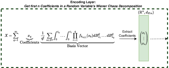
(a) Encoding Layer

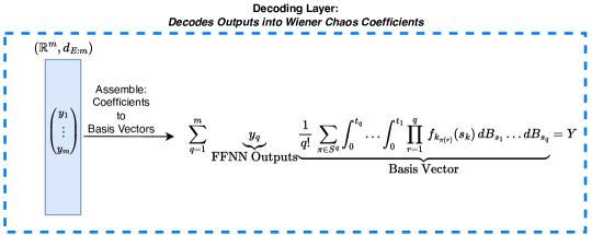
(b) Decoding Layer

Figure 5: Illustration of our “static” operator network in Definition 7 specialized to the geometry of the input space $L^{2}(\Omega,\mathcal{G}_{T},\mathbb{P})$ and the output space $L^{2}(\Omega,\mathcal{F}_{t},\mathbb{P})$; for $\sigma$ algebras $\mathcal{G}$ and $\mathcal{F}$ on a sample space $\Omega$. The network is works in three phases. 1) First inputs are encoded as finite-dimensional Euclidean data by mapping them to their truncated (Schauder) basis coefficients in the input space $E$. 2) Next these coefficients are transformed by a ReLU FFNN. 3) The outputs of ReLU FFNN’s output are interpreted as coefficients a Wiener Chaos expansion a truncated (Schauder) basis in the output space $F$.

4.1 A primer on Wiener Chaos

We fix a probability space $\big{(}\Omega,\mathcal{F},\mathbb{P}\big{)}$ supporting a standard one dimensional Brownian motion $(B_{t})_{t\geq 0}$ and let $\mathbb{F}\stackrel{{\scriptstyle\mbox{\tiny def.}}}{{=}}(\mathcal{F}_{t})_{t\geq 0}$ denote the complete and right-continuous enlargement of the filtration generated by $(B_{t})_{t\geq 0}$. We recall that the Ito (stochastic) integral of a (deterministic) simple function $f=\sum_{i=1}^{k}\,\beta_{i}I_{[0,t_{i}]}$ in $L^{2}([0,t])$, where $0\leq t_{1}<\dots<t_{k}\leq t$ is the Gaussian random variable

$$\int_{0}^{t}\,f(s)\,dB_{s}\stackrel{{\scriptstyle\mbox{\tiny def.}}}{{=}}\sum_{i=1}^{k}\,\beta_{i}\,\big{(}B_{t_{i}}-B_{t_{i-1}}\big{)}.$$ (20)

More generally, the Ito integral of any function $f\in L^{2}([0,t])$ is defined as the limit in $L^{2}(\Omega,\mathcal{F}_{t},\mathbb{P})$ of a sequence $\{\int_{0}^{t}\,f_{k}(s)\,dB_{s}\}_{k=1}^{\infty}$ where the $\{f_{k}\}_{k=1}^{\infty}$ is any choice of simple integrands converging to $f$ in $L^{2}([0,t])$. Thus, $\int_{0}^{t}\,f(s)\,dB_{s}$ is a centered normal random variable with variance $\int_{0}^{t}\,f^{2}(s)\,ds$. We also note that such a sequence always exists and $\int_{0}^{t}\,f(s)\,dB_{s}$ is independent of the particular choice of the approximating sequence $\{f_{k}\}_{k=1}^{\infty}$.

Using tools common to (Malliavin) stochastic calculus we may exhibit an orthonormal basis of $L^{2}(\Omega,\mathcal{F}_{t},\mathbb{P})$. We refer the interested reader to nualart2006malliavin for a more detailed discussion on this construction. This construction relies on a system of orthogonal polynomials $\{h_{k}\}_{k=1}^{\infty}$ known as Hermite polynomials and defined by the recurrence relation

$$h_{k+1}(x)=xh_{k}(x)-h_{k}^{\prime}(x),$$

where $h_{0}(x)\stackrel{{\scriptstyle\mbox{\tiny def.}}}{{=}}1$. For instance, $h_{1}(x)=x$, $h_{2}(x)=x^{2}-1$, and so on.

By means of the Ito stochastic integral and the Hermite polynomials we may define the $q^{th}$ Wiener Chaos to be the subspace $\mathcal{H}_{t}^{q}$ of $L^{2}(\Omega,\mathcal{F}_{t},\mathbb{P})$ spanned by the random variables of the form

$$I^{q}(f)\stackrel{{\scriptstyle\mbox{\tiny def.}}}{{=}}h_{q}\biggr{(}\int_{0}^{t}\,f(s)\,dB_{s}\biggl{)},$$

where $f\in L^{2}([0,t])$, where $q\in\mathbb{N}_{+}$ and $\mathcal{H}_{t}^{0}\stackrel{{\scriptstyle\mbox{\tiny def.}}}{{=}}\mathbb{R}$. The Wiener chaos $(\mathcal{H}_{t}^{q})_{q=0}^{\infty}$ produces an orthogonal decomposition, given in (nualart2006malliavin, , Theorem 1.1.1), of $L^{2}(\Omega,\mathcal{F}_{t},\mathbb{P})$, meaning that for each pair of random variables $Y_{q}\in\mathcal{H}_{t}^{q}$ and $Y_{\tilde{q}}\in\mathcal{H}_{t}^{\tilde{q}}$ are orthogonal in $L^{2}(\Omega,\mathcal{F}_{t},\mathbb{P})$ whenever $q\neq\tilde{q}$; every random variable $Y\in L^{2}(\Omega,\mathcal{F}_{t},\mathbb{P})$ can uniquely be decomposed as

$$Y=\sum_{q=0}^{\infty}\,Y_{q},$$

where $Y_{q}\in\mathcal{H}_{t}^{q}$ for each $q\in\mathbb{N}$ and where the sum converges in $L^{2}(\Omega,\mathcal{F}_{t},\mathbb{P})$.

Since the Wiener Chaos is an orthogonal decomposition of $L^{2}(\Omega,\mathcal{F}_{t},\mathbb{P})$ then the union of any set of orthogonal basises of each $\mathcal{H}_{t}^{q}$ is an orthogonal basis of $L^{2}(\Omega,\mathcal{F}_{t},\mathbb{P})$ itself. Therefore, we only need to exhibit an orthogonal basis of each $\mathcal{H}_{t}^{q}$ for $q\in\mathbb{N}_{+}$.

We leverage the symmetrized tensor product of elements $f_{1},\dots,f_{q}\in L^{2}([0,t])$ defined by

$$\operatorname{sym}\big{(}f_{1}\otimes\dots\otimes f_{q}\big{)}\stackrel{{\scriptstyle\mbox{\tiny def.}}}{{=}}\frac{1}{q!}\,\sum_{\pi\in S^{q}}\,f_{\pi(1)}\otimes\dots\otimes f_{\pi(q)}$$

where $S^{q}$ is the set of permutations of the indices $\{1,\dots,q\}$. More concretely, the Hilbert space generated by the symmetrized tensor product is identified with the set of symmetric functions in $L^{2}([0,t]^{q})$ which we denote by $L^{2}_{\operatorname{sym}}([0,t]^{q})$. Since the $q$-fold symmetrized tensor product is a subspace of the (usual) $q$-fold tensor product then the identification of the $q$-fold symmetric tensor product of $L^{2}([0,t])$ with $L^{2}_{\operatorname{sym}}([0,t]^{q})$ may be further simplified to

$$\operatorname{sym}\big{(}f_{1}\otimes\dots\otimes f_{q}\big{)}\,\leftrightarrow\frac{1}{q!}\,\sum_{\pi\in S^{q}}\,\prod_{i=1}^{q}\,f_{\pi(i)}(s_{i}).$$

The connection between the symmetrized tensor product and the $q^{th}$ Wiener Chaos is that the $q^{th}$ Wiener Chaos $\mathcal{H}_{t}^{q}$ is structurally identical to $L^{2}_{\operatorname{sym}}([0,t]^{q})$ (identified with the $q$-fold symmetrized tensor product of $L^{2}_{\operatorname{sym}}([0,t])$ with itself). The map realizing this identification sends any $f\in L^{2}_{\operatorname{sym}}([0,t]^{q})$ to its $q$-fold multiple stochastic integral

$$f\mapsto\int_{0}^{t_{q}}\dots\int_{0}^{t_{1}}\,f(s_{1},\dots,s_{q})\,dB_{s_{1}}\dots dB_{s_{q}}.$$ (21)

Moreover, the map (21) is linear isometric isomorphism preserving inner products. Consequentially, any orthogonal basis of $L^{2}_{\operatorname{sym}}([0,t]^{q})$ is sent to an orthogonal basis of $\mathcal{H}_{t}^{q}$ under this identification. Since an orthogonal basis of $L^{2}_{\operatorname{sym}}([0,t]^{q})$ is given by the set

$$\operatorname{sym}\big{(}f_{1}\otimes\dots\otimes f_{q}\big{)}$$

where $\{f_{i}\}_{i=1}^{\infty}$ is an orthogonal basis of $L^{2}([0,t])$ then the identification (21) implies that the corresponding set of random variables

$$\int_{0}^{t_{q}}\dots\int_{0}^{t_{1}}\,\operatorname{sym}\big{(}f_{1}\otimes\dots\otimes f_{q}\big{)}(s_{1},\dots,s_{q})\,dB_{s_{1}}\dots dB_{s_{q}},$$ (22)

is an orthogonal basis of the $q^{th}$ Wiener Chaos $\mathcal{H}_{t}^{q}$. Such an orthogonal basis of $L^{2}([0,t])$ is given by the Fourier basis whose elements are

$$f_{j,i}(x)\stackrel{{\scriptstyle\mbox{\tiny def.}}}{{=}}\begin{cases}\sqrt{\frac{2}{t}}\sin\left(\frac{j\pi x}{t}\right)&\mbox{if }\,i\mbox{ = 0}\\ \sqrt{\frac{2}{t}}\cos\left(\frac{(j-1)\pi x}{t}\right)&\mbox{if }\,i\mbox{ = 1},\end{cases}$$

where $j\in\mathbb{N}_{+}$ and $i\in\{0,1\}$. For convenience, with some abuse of notation, we denote an enumeration of $\{f_{i,j}\}_{i\in\mathbb{N},j\in\{0,1\}}$ by $\{f_{k}\}_{k=1}^{\infty}$. Consequentially, an orthogonal basis of $L^{2}(\Omega,\mathcal{F}_{t},\mathbb{P})$ is given by the countable family of random variables

$$Z_{(k_{1},\dots,k_{q})}\stackrel{{\scriptstyle\mbox{\tiny def.}}}{{=}}\frac{1}{q!}\,\sum_{\pi\in S^{q}}\,\int_{0}^{t_{q}}\dots\int_{0}^{t_{1}}\prod_{r=1}^{q}\,f_{k_{\pi(r)}}(s_{k})\,dB_{s_{1}}\dots dB_{s_{q}},$$

where $(k_{1},\dots,k_{q})$ is a multi-index belonging to $\mathcal{A}\stackrel{{\scriptstyle\mbox{\tiny def.}}}{{=}}\bigcup_{q=0}^{\infty}\,\mathbb{N}^{q}$; we also make the convention that $Z_{\varnothing}\stackrel{{\scriptstyle\mbox{\tiny def.}}}{{=}}1$, and we have used the linearity of the Ito (stochastic) integral in conjunction with the above considerations.

4.2 Simultaneous Approximation of SDEs with Different Initial Conditions using CNOs

Monte Carlo methods allow for the efficient solution to stochastic differential equations (SDEs) with a convergence rate of $\mathcal{O}(1/\sqrt{S})$ to the true solution, where $S$ is the number of samples, plus a comparable discretization error when resorting to a tamed Euler scheme JenztenTamedEulre2011 . It is known that deep learning can provide a suitable alternative to Monte Carlo schemes by learning the SDE’s solution map given deterministic initial conditions, for a fixed terminal time, by efficiently approximating the solutions to their associated PDEs Beck2018 given by the Feynman-Kac Theorem.

In this section, we show how a single CNO can be used for efficient simultaneously solving SDEs with various noisy initial conditions across different time-horizons, by simultaneously approximately learning solve a family of stochastic differential equations with many different stochastic initial conditions and different initial times.

This section’s application shows that the CNO can approximate causal maps with stochastic inputs on arbitrarily long time horizons. This extends the known guarantees for recurrent neural networks, specifically reservoir computers, which can approximate time-invariant causal maps Lukas_StochInputReservoir .

We are given a non-degenerate time grid $(t_{n})_{n\in\mathbb{Z}}$ as in Assumption 3.1.1, $\beta$ and $\alpha$ in $C([0,\infty)\times\mathbb{R},\mathbb{R})$ such that there exists $M>0$ such that for all $t\geq 0$ and all $x_{1},x_{2}\in\mathbb{R}$, we have

$$|\beta(t,x_{1})-\beta(t,x_{2})|^{2}+|\alpha(t,x_{1})-\alpha(t,x_{2})|^{2}\leq M^{2}|x_{1}-x_{2}|$$ (23)

$$|\beta(t,x_{1})|^{2}+|\alpha(t,x_{1})|^{2}\leq M^{2}(1+|x_{1}|^{2}).$$ (24)

Theorem 8.7 in DaPrato2008 guarantees that for all $i\in\mathbb{N}_{+}$, under the growth conditions (23) and (24), for $\eta\in L^{2}(\Omega,\mathcal{F}_{t_{i}},\mathbb{P})$ there exists a unique $X\in C([t_{i},t_{i+1}];L^{2}(\Omega,\mathcal{F}_{t_{i+1}},\mathbb{P}))$ which satisfies $\mathbb{P}$-a.s.

$$X_{t_{i+1}}=\eta+\int_{t_{i}}^{t_{i+1}}\alpha(s,X_{s})\,ds+\int_{t_{i}}^{t_{i+1}}\beta(s,X_{s})\,dB_{s},$$ (25)

where we set $X_{t_{i}}=\eta$; in what follows, we will indicate the explicit dependence on $\eta$ in $X_{t_{i+1}}$, i.e. $X_{t_{i+1}}^{\eta}$. Therefore, $\forall i\in\mathbb{N}_{+}$ the following (non-linear) solution operator

$$\operatorname{SDE-Solve}_{t_{i}:t_{i+1}}\,:\,L^{2}(\Omega,\mathcal{F}_{t_{i}},\mathbb{P})\rightarrow L^{2}(\Omega,\mathcal{F}_{t_{i+1}},\mathbb{P}),\quad\eta\rightarrow X_{t_{i+1}}^{\eta}$$ (26)

is well defined. To see that each of the maps $\operatorname{SDE-Solve}_{t_{i}:t_{i+1}}$ satisfies the assumptions of our theorems, it is sufficient to note that under (23) and (24), the operator $\operatorname{SDE-Solve}_{t_{i}:t_{i+1}}$ is Lipschitz and, in view of (DaPrato2008, , Proposition 8.15), it belongs to the trace-class $C_{1,\text{tr}}^{\lambda}(K,L^{2}(\Omega,\mathcal{F}_{t_{i+1}},\mathbb{P}))$ for all compact subsets $K$ of $L^{2}(\Omega,\mathcal{F}_{t_{i}},\mathbb{P})$, since

$$\begin{split}\|X_{t_{i+1}}^{\hat{\eta}}-X_{t_{i+1}}^{\tilde{\eta}}\|_{L^{2}(\Omega,\mathcal{F}_{t_{i+1}},\mathbb{P};\mathbb{R})}&\leq\sqrt{3}e^{\frac{3}{2}M^{2}(t_{i+1}-t_{i}+1)(t_{i+1}-t_{i})}\|\hat{\eta}-\tilde{\eta}\|_{L^{2}(\Omega,\mathcal{F}_{t_{i}},\mathbb{P};\mathbb{R})}\\ &\leq\sqrt{3}e^{\frac{3}{2}M^{2}(\Delta^{+}+1)\Delta^{+}}\|\hat{\eta}-\tilde{\eta}\|_{L^{2}(\Omega,\mathcal{F}_{t_{i}},\mathbb{P};\mathbb{R})}.\end{split}$$ (27)

with $\lambda\leq\sqrt{3}e^{\frac{3}{2}M^{2}(\Delta^{+}+1)\Delta^{+}}$ and $\Delta^{+}\stackrel{{\scriptstyle\mbox{\tiny def.}}}{{=}}\sup_{i\in\mathbb{Z}}\Delta t_{i}<\infty$ as in Assumption 3.1.1.

We consider the causal map

$$\begin{split}\operatorname{SDE-Solve}\,:\,&\left(\prod_{i\in\mathbb{Z};t_{i}<0}\{0\}\right)\times\prod_{i\in\mathbb{Z};t_{i}\geq 0}\,L^{2}(\Omega,\mathcal{F}_{t_{i}},\mathbb{P})\rightarrow\left(\prod_{i\in\mathbb{Z};t_{i}<0}\{0\}\right)\times\prod_{i\in\mathbb{Z};t_{i}\geq 0}L^{2}(\Omega,\mathcal{F}_{t_{i}},\mathbb{P}),\\ &\quad\quad\quad\quad\quad\quad\,\,(\eta_{t_{i}})_{i\in\mathbb{Z}}\mapsto\operatorname{SDE-Solve}\left[(\eta_{t_{i}})_{i\in\mathbb{Z}}\right],\end{split}$$ (28)

$$\left(\operatorname{SDE-Solve}\left[(\eta_{t_{i}})_{i\in\mathbb{Z}}\right]\right)_{j}=\begin{cases}0,\quad\text{if }t_{j}<0\\ \operatorname{SDE-Solve}_{t_{j}:t_{j+1}}(\eta_{t_{j}}),\quad\text{if }t_{j}\geq 0,\end{cases}$$ (29)

where each $\operatorname{SDE-Solve}_{t_{i}:t_{i+1}}(\eta_{t_{i}})$ is defined as in Equation (26). The typical example which we have in mind, in the following, are input sequences which are orbits of square-integrable random variables under the an SDE’s solution operator; i.e.

$$\eta_{t_{i+1}}=\operatorname{SDE-Solve}_{t_{i}:t_{i+1}}(\eta_{t_{i}})\mbox{ and }\eta_{t_{0}}=X,$$ (30)

for some $X\in L^{2}(\Omega,\mathcal{F}_{0},\mathbb{P})$. Thus, approximating $\operatorname{SDE-Solve}$ and applying it to any compact subset of the path-space comprised of elements of the form (30) corresponds to simultaneously solving an SDE for several random initial conditions across arbitrarily time-intervals beginning at several initial times.

By Equation (27), $\operatorname{SDE-Solve}$ is a causal map as in Definition (9), since in this case we can simply take $r=0,\alpha=1$, $M=1$, $f_{t_{i}}=\operatorname{SDE-Solve}_{t_{i}:t_{i+1}}$, and $\lambda\leq\sqrt{3}e^{\frac{3}{2}M^{2}(\Delta^{+}+1)\Delta^{+}}$ holds for any $i\in\mathbb{N}_{+}$. Theorem 3.2 guarantees that there exists a CNO which approximates the map in Equation (28), as soon as we confine ourselves on a compact path space. Let us summarize our findings in

Corollary 1 (Causal Universal Approximation of SDEs with Stochastic Dynamics)

Consider the setting of this section and fix the path space

$$\mathcal{X}\stackrel{{\scriptstyle\mbox{\tiny def.}}}{{=}}\left(\prod_{i\in\mathbb{Z};t_{i}<0}\{0\}\right)\times\prod_{i\in\mathbb{Z};t_{i}\geq 0}\,\mathcal{X}_{t_{i}},$$

where each $\mathcal{X}_{t_{i}}$ is a compact subset of $L^{2}(\Omega,\mathcal{F}_{t_{i}},\mathbb{P})$. Then the operator $\operatorname{SDE-Solve}$

$$\operatorname{SDE-Solve}\,:\,\left(\prod_{i\in\mathbb{Z};t_{i}<0}\{0\}\right)\times\prod_{i\in\mathbb{Z};t_{i}\geq 0}\,\mathcal{X}_{t_{i}}\rightarrow\left(\prod_{i\in\mathbb{Z};t_{i}<0}\{0\}\right)\times\prod_{i\in\mathbb{Z};t_{i}\geq 0}L^{2}(\Omega,\mathcal{F}_{t_{i}},\mathbb{P})$$

is $(0,1,\sqrt{3}e^{\frac{3}{2}M^{2}(\Delta^{+}+1)\Delta^{+}})$-Hölder.

Given $Q,\delta\in\mathbb{N}_{+}$, an “encoding error" $\varepsilon_{D}>0$ and an “approximation error" $\varepsilon_{A}>0$ there exist a multi-index $[d]$, a “latent code" $z_{0}\in\mathbb{R}^{P([d])+Q}$, a linear readout map $L\,:\,\mathbb{R}^{P([d])+Q}\rightarrow\mathbb{R}^{P([d])}$, and a ReLU FFNN $\hat{h}\,:\,\mathbb{R}^{P([d])+Q}\rightarrow\mathbb{R}^{P([d])+Q}$ such that the sequence of parameters $\theta_{t_{i}}\in\mathbb{R}^{P([d])}$ defined recursively

$$\begin{split}\theta_{t_{i}}\stackrel{{\scriptstyle\mbox{\tiny def.}}}{{=}}L(z_{t_{i}})\\ z_{t_{i+1}}\stackrel{{\scriptstyle\mbox{\tiny def.}}}{{=}}\hat{h}(z_{t_{i}}),\end{split}$$

with $i$ belongs to $[[I]]\cup\{0\}$ provided by the definition of causal maps , satisfies to the following uniform estimates:

$$\begin{split}\max_{i\in[[I]]}\,\sup_{X_{\cdot}\in\mathcal{X}}\,\,\|\hat{f}_{t_{i}}(X_{(t_{i-1},t_{i}]})-\operatorname{SDE-Solve}(X_{\cdot})_{t_{i}}\|_{L^{2}}<\varepsilon_{A}+\varepsilon_{D},\end{split}$$

where $\hat{f}_{t_{i}}\in\mathcal{NF}_{[n_{\varepsilon_{D}}]}^{(P)ReLU}$ Moreover, for the hyperparameter $n_{\varepsilon_{D}}^{in}$ it holds

$$n_{\varepsilon_{D}}^{in}=\inf\left\{n\in\mathbb{N}_{+}:\max_{x\in\mathcal{X}}d_{E}(A_{E:n}(x),x)\leq\frac{\varepsilon_{D}}{2\lambda}\right\}$$

where we have set $E\stackrel{{\scriptstyle\mbox{\tiny def.}}}{{=}}\Pi_{i\in\mathbb{Z}}L^{2}(\Omega,\mathcal{F}_{t_{i}},\mathbb{P})$.

4.3 Discussion - Corollary 1: Jumps, Path-Dependence, and Accelerated Approximation Rates Under Smoothness

We briefly discuss some points surrounding Corollary 1. For instance, how the result allows for stochastic discontinuity-type jumps. We also discuss how the scope of Theorem 3.1 allows for Corollary 1 to be easily generalized; but we opt not to do that in this manuscript, rather opting for a less technical illustration of our general framework.

Improved Approximation Rates for SDEs Driven by Smooth Coefficients

If, in addition to conditions (24) and (23), the drift and diffusion coefficients $\alpha$ and $\beta$ are sufficiently differentiable, then (RosestolatoBook2017, , Theorem 3.9) implies that each of the maps $\operatorname{SDE-Solve}_{t_{i}:t_{i+1}}$ are $C^{k}$. Whence, the operator $\operatorname{SDE-Solve}$ is a smooth causal map of finite virtual memory. Thus, in this case, Theorem 3.2 implies improved approximation rates by the CNO model.

Stochastic Discontinuities at Time-Grid Points

We highlight that the adapted map $\operatorname{SDE-Solve}$ does accommodate jumps but only if those jumps occur on the fixed time-grid points $\{t_{i}\}_{i\in\mathbb{N}}$. Such constructions have recently appeared in the rough path literature Allan2021ArXiV and the causal/functional Itô calculus literature Cont2022JMathAnnAppl .

In financial applications, the possibility of a stochastic process’ to jump at predetermined times (called stochastic discontinuities in that context) are an essential ingredient of accurately modeling interest rates; for example, European reference interest rates typically exhibit jumps directly after monetary policy meetings of ECB Font2020FinStoch .

Path Dependent Dynamics

One could consider SDEs driven with path dependant random drift and diffusion coefficients, since all that is needed to apply Theorem 3.2 is the regularity of the $\operatorname{SDE-Solve}$ operator; which is guaranteed by results such as DePrato2016AnnProb or RosestolatoBook2017 . However, we instead opted for a simple first presentation, explicitly illustrating the scope of our results in this easier case.

5 The Benefit of Causal Approximation: Super-Optimal Approximation Rates for Causal Maps

We now illustrate the quantitative advantage of causal approximation, i.e. using our CNO architecture, when the target function is causal. For illustrative purposes, we consider the simplest case where all involved spaces are finite-dimensional and Euclidean. By considering this setting, we can juxtapose our approximation rates derived from Theorem 3.2 against the best rates for ReLU networks ZHS2022JMPA which are optimal, as shown in the constructive approximation literature DVL1993 ; Grohs2021IEEETransInfoTheory . Therefore, when the target function has a causal structure, “super-optimal uniform approximation rates” can be achieved only if one encodes that structure into the neural network model; as in the case with the CNO. Throughout this section, we consider the integer time-grid $\{t_{i}\}_{i\in\mathbb{Z}}=\{t\}_{t\in\mathbb{Z}}$; which we note satisfies the non-degeneracy condition in Assumption 3.1.1.

5.1 In the Euclidean Case, CNOs are a simple class of RNNs which are universal dynamical systems

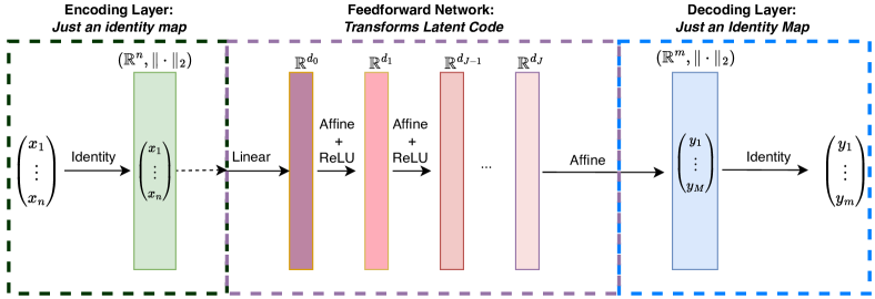
Figure 6: Neural Filters - Euclidean Spaces: If the input and output spaces are Euclidean, then the projection and reconstruction layers in Figure 3 can be dropped; since they reduce to formal identity maps. Thus, in this setting a neural filter is a deep ReLU FFNN.

In KN1998NN , the authors investigate the problem of approximating a dynamical system on a Euclidean space by a RNN. In their most general form, RNNs – sometimes also called “fully RNN", or fRNNs - are given for times $t>0$ by

$$\begin{split}y_{t}&\stackrel{{\scriptstyle\mbox{\tiny def.}}}{{=}}\hat{f}_{\theta_{t}}(y_{t-1},x_{t}),\\ y_{0}&\stackrel{{\scriptstyle\mbox{\tiny def.}}}{{=}}y,\end{split}$$ (31)

where $y_{t}$ is the state of the system, $x_{t}$ is an external input, $y$ the initial state, and $\hat{f}_{\theta_{t}}$ are (possibly deep) FFNNs with a priori no relationship among their parameters $(\theta_{t})_{t\in\mathbb{N}_{+}}$. In particular, each FFNNs may have different depth and/or width. However, in practice, restrictions are put on the sequence of networks $(\hat{f}_{\theta_{t}})_{t\in\mathbb{N}_{+}}$; precisely, it is usually required that they all have the same complexity, and each $\theta_{t+1}$ is recursively determined from the pair $(\theta_{t},x_{t})$. For instance, if it is only assumed that each FFNNs in Equation (31) has the same complexity, then the classical result of SS1995JCSS shows that one may simulate all Turing Machines by fRNNs with rational weights and biases. Although this result is promising for the expressive power of fRNNs, it is far removed from any practical model since it places absolutely no restriction on how the sequence $(\theta_{t})_{t\in\mathbb{N}_{+}}$ is determined. As a consequence, the model in Equation (31) is not implementable since it depends on an infinite number of parameters, as there is no relationship between $\theta_{t}$ and any $\theta_{s}$ for all past times $s<t$. On the other extreme, a very recent paper helmut2022metric prove that a RNN with a single hidden layer and with $\theta_{t}=\theta_{0}$, for all $t\in\mathbb{N}_{+}$, can approximate linear time-invariant dynamical systems quantitatively.
Still, surprisingly, many questions surrounding the approximation power of more sophisticated but implementable RNNs remain open. For instance, the ability of such RNNs to approximate non-linear dynamical systems, quantitatively, and the quantitative role of the hidden state space/latent code’s dimension are still open problems in the neural network literature. This subsection, addresses these open problems as a simple and direct consequence of Theorem 3.2.
This is because if $E=B=\mathbb{R}^{d}$, (with $\mathbb{R}^{d}$ equipped with the Euclidean distance), then our CNO model defines a very simple RNN. In order to see this, let $(e_{i})_{i=1}^{d}$ be the standard basis of $\mathbb{R}^{d}$, which is trivially a Schauder basis for the latter. Requiring that the encoding and the decoding dimensions of our CNO model are at least $d$, we have that the latter is given by:

$$\begin{cases}y_{t}\stackrel{{\scriptstyle\mbox{\tiny def.}}}{{=}}\hat{f}_{\theta_{t}}(x_{t}),\\ \theta_{t}\stackrel{{\scriptstyle\mbox{\tiny def.}}}{{=}}L(z_{t}),\\ z_{t+1}\stackrel{{\scriptstyle\mbox{\tiny def.}}}{{=}}\hat{h}(z_{t}).\end{cases}$$ (32)

Moreover, by pre-composing each $\hat{f}_{\theta_{t}}$ in Equation (32) with the following linear projection

$$A\,:\,\mathbb{R}^{N}\times\mathbb{R}^{N}\rightarrow\mathbb{R}^{N},\quad(y,x)\rightarrow x,$$

and by noting that $\hat{f}_{\theta_{t}}\circ A$ is a FFNN because of the invariance with respect the pre-composition by affine functions, we have that the CNO becomes

$$\begin{cases}y_{t}\stackrel{{\scriptstyle\mbox{\tiny def.}}}{{=}}\hat{f}_{\theta_{t}}(y_{t-1},x_{t}),\quad y_{0}\stackrel{{\scriptstyle\mbox{\tiny def.}}}{{=}}y\\ \theta_{t}\stackrel{{\scriptstyle\mbox{\tiny def.}}}{{=}}L(z_{t}),\\ z_{t+1}\stackrel{{\scriptstyle\mbox{\tiny def.}}}{{=}}\hat{h}(z_{t}),\end{cases}$$ (33)

where with a minor abuse of notation we keep using $\hat{f}_{\theta_{t}}$ instead of $\hat{f}_{\theta_{t}}\circ A$. By comparing Equations (31) and (33), we see that the CNO model is a RNN whose weights and biases do not depend upon the input sequence $(x_{t})_{t\in\mathbb{N}_{+}}$, and are determined recursively by the hypernetwork $\hat{h}$, as in HDQICLR2017 . Therefore, our CNO is essentially the classical Elman RNN of EL1990 with $\hat{f}_{\theta_{t}}$ and $\hat{h}$ having several, instead of one, hidden layer.
We now illustrate the expressive power of the CNO model in Equation (33). For simplicity, we consider the case of dynamical system defined on a smooth compact sub-manifold $\mathcal{M}$ of $\mathbb{R}^{d}$, possibly with boundary; these types of dynamical systems arise often in physics DynamicsPhys ; HamiltonianOrtega and are actively studied in the reservoir computing literature Takens2022 . We let $(g_{t})_{t\in\mathbb{N}}$ be a sequence of smooth functions from $\mathbb{R}^{d}$ to itself which fix the manifold $\mathcal{M}$, namely, $g_{t}(\mathcal{M})\subseteq\mathcal{M}$ for every $n\in\mathbb{N}$. We further require that the family $(g_{t})_{t\in\mathbb{N}}$ has uniformly bounded gradient on $\mathcal{M}$; meaning that for some $\lambda\geq 0$ it holds

$$\sup_{t\in\mathbb{N}}\,\max_{x\in\mathcal{M}}\,\|\nabla g_{t}(x)\|\leq\lambda.$$

NB, this is of-course satisfied by any autonomous dynamical system; namely when $g_{t}=g_{0}$ for all integers $t$, with $g_{0}$ smooth.

Then the restriction of each $g_{t}$ to $\mathcal{M}$ defines a dynamical system and we can express the causal structure in the orbit of any initial state $x_{0}\in\mathcal{M}$ evolving under $g$ as a smooth causal map. To see this, consider the path space $\mathcal{X}$ whose elements are sequences $x_{\cdot}\in\mathcal{M}^{\mathbb{Z}}$ of the following form

$$x^{(t)}\stackrel{{\scriptstyle\mbox{\tiny def.}}}{{=}}\begin{cases}g_{t}\circ\ldots\circ g_{0}(x_{0})&\mbox{if }t>0\\ x_{0}&\mbox{if }t\leq 0.\\ \end{cases}$$

Now, let $\mathcal{Y}\stackrel{{\scriptstyle\mbox{\tiny def.}}}{{=}}(\mathbb{R}^{d})^{\mathbb{Z}}$. Then, by construction, we immediately deduce that the operator $f\,:\,\mathcal{X}\rightarrow\mathcal{Y}$ defined as

$$f(x_{\cdot})_{t}\stackrel{{\scriptstyle\mbox{\tiny def.}}}{{=}}\begin{cases}g_{t}(x^{(t)})&\mbox{if }t>0\\ x_{0}&\mbox{if }t\leq 0,\\ \end{cases}$$ (34)

defines a $(0,\infty,\lambda)$-smooth causal map.

The Quantitative Advantage of the Hypernetwork for Approximating Causal Maps

We fix a positive integer $T$ and a $1$-Lipschitz function $G:\mathbb{R}^{2}\rightarrow[0,1]$. For any input sequence $(z_{t})_{t=1}^{T}\in[0,1]^{T}$ define the output sequence $(z^{(t)})_{t=1}^{T}\in[0,1]^{T}$ by

$$z^{(t)} \stackrel{{\scriptstyle\mbox{\tiny def.}}}{{=}}G(z_{t},z^{(t-1)}), \qquad t=1,\dots,T,$$ (35)

where we set $z^{(0)}\stackrel{{\scriptstyle\mbox{\tiny def.}}}{{=}}0$. We define the map $f:[0,1]^{T}\rightarrow\mathbb{R}$ as follows

$$f(z_{1},\dots,z_{T})\stackrel{{\scriptstyle\mbox{\tiny def.}}}{{=}}z^{(T)}=G(z_{T},z^{(T-1)}).$$

Evidently, $f$ is causal, whence, it can be approximated both by the CNO model or by a neural filter (which in this setting reduces to a deep ReLU FFNN). Comparing the approximation rates in either case in Tables 2 and 1 we see that an approximation by a deep ReLU network (i.e. a neural filter in this case) requires a depth of $\tilde{O}(\epsilon_{A}^{-2/T})$ and a width of $\tilde{O}(\epsilon_{A}^{-2/T})$ to approximate $f$ uniformly on $[0,1]^{T}$ to a maximal error of $\epsilon_{A}$. In contrast, a CNO model only requires a latent state dimension $P([d])+Q=\tilde{O}(\epsilon_{A}^{-6}-\log_{1/2}(T-1))$ with hypernetwork $\hat{h}$ of depth $\tilde{O}(T^{3/2})$ and width $\tilde{O}(\epsilon_{A}^{-6}-\log_{1/2}(T-1)T)$ in order to achieve the same uniform approximation of $f$ on $[0,1]^{T}$ with a maximal error of $\epsilon_{A}$.
As shown in (ZHS2022JMPA, , Theorem 2.4), the ReLU feedforward networks achieve the optimal approximation rates when approximating arbitrary Lipschitz functions, then, our rates in Theorem 3.2 imply that the CNO achieves super-optimal rates when approximating generic Lipschitz functions of the form in (35). Moreover, a direct examination of the above rates shows that the CNO is not cursed by dimensionality when measured in the number of time steps one wishes the uniform approximation to hold for, while deep ReLU FFNNs are. Consequently, this shows that CNOs are highly advantageous for (causal) sequential learning tasks from the approximation theoretic perspective.

6 Conclusion

We presented a first universal approximation theorem which is both causal, quantitative, compatible with infinite-dimensional operator learning, and which is not restricted to “function spaces” but is compatible with general “good” infinite-dimensional linear metric spaces. Our main contributions, Theorem 3.1 and Theorem 3.2, provided approximation guarantees for any smooth or Hölder (non-linear) operator between Fréchet spaces in the “static” or “causal” case, where temporal structure is or is not present in the approximation problem, respectively.

We showed how the CNO model can approximate a variety of solution operators, and infinite dimensional dynamical systems, arising in stochastic analysis. Moreover, in the Euclidean case, we showed that our neural filter’s approximation rates are optimal. We then showed that, when the target operator being approximated is a dynamical system, then the CNO’s approximation rates are super-optimal. Optimality is quantified in terms of the number of parameters required to approximate any arbitrary map belonging to some broad class as in constructive approximation theory of DVL1993 .

We believe the observations made in this work open up avenues for future literature. As a prime example, we would like to further optimize our CNO for the stochastic filtering problem assuming additional structural conditions. As future work, we aim to build on these results in the context of robust finance.

Appendix A Background material for proofs

In an effort to keep the paper as self-contained as possible, this appendix contains any background material required in the derivations of our main results but not required for their formulation. We cover various properties of deep ReLU neural networks, covering and packing results, and we overview some properties of finite-dimensional “linear dimension reduction” techniques in well-behaved Fréchet spaces. We also include a list of some useful properties of generalized inverses.

A.1 Neural Network Regressors

This section contains auxiliary results on neural network approximation, parallelization, and memorization.

A.1.1 DNN Approximation for Smooth and Hölder Functions

Theorem 1.1 in JZHS2021SIAM proves that ReLU FFNNs with width $\mathcal{O}(N\,\log(N))$ and depth $\mathcal{O}(L\,\log(L)+d)$ can approximate a function $f\in C^{s}([0,1]^{d})$ with a nearly optimal approximation error $\mathcal{O}(\|f\|_{C^{s}([0,1]^{d})}\,N^{-2s/d}\,L^{-2s/d})$, where the norm $\|\cdot\|_{C^{s}([0,1]^{d})}$ is defined as:

$$\|f\|_{C^{s}([0,1]^{d})}\stackrel{{\scriptstyle\mbox{\tiny def.}}}{{=}}\max\{\|\partial^{\boldsymbol{\alpha}}f\|_{L^{\infty}([0,1]^{d})}\,:\,|\boldsymbol{\alpha}|\leq s,\,\boldsymbol{\alpha}\in\mathbb{N}^{d}\},\quad f\in C^{s}([0,1]^{d}).$$ (36)

More precisely, they state and prove the following

Theorem A.1 (JZHS2021SIAM )

Given a function $f\in C^{s}([0,1]^{d},\mathbb{R})$ with $s\in\mathbb{N}_{+}$, for any $N,L\in\mathbb{N}_{+}$, there exists a function $\varphi$ implemented by a ReLU FFNN with width $C_{1}\,(N+2)\,\log_{2}(8N)$ and depth $C_{2}\,(L+2)\,\log_{2}(4L)+2d$ such that

$$\|\varphi-f\|_{L^{\infty}([0,1]^{d})}\leq C_{3}\,\|f\|_{C^{s}([0,1]^{d})}\,N^{-2s/d}\,L^{-2s/d},$$ (37)

where $C_{1}=17s^{d+1}3^{d}d$, $C_{2}=18s^{2}$ and $C_{3}=85(s+1)^{d}8^{s}$.

In particular, note that the previous result does not privilege the width to the depth and vice versa because the exponent for both $N$ and $L$ on the right-hand side of Equation (37) is $-2s/d$.
On the other hand, ZHS2022JMPA , as a consequence of their main theorem for explicit error characterization, state and prove the following.

Theorem A.2 (ZHS2022JMPA )

Given a Hölder continuous function on $[0,1]^{d}$ of order $\alpha\in(0,1]$ with Hölder constant $\lambda>0$, i.e., $f\in C^{\lambda}_{\alpha}([0,1]^{d},\mathbb{R})$, then for any $N\in\mathbb{N}_{+}$, $L\in\mathbb{N}_{+}$ and $p\in[1,\infty]$, there exists a function $\varphi$ implemented by a ReLU network with width $C_{1}\max\{d\lfloor N^{1/d}\rfloor,N+2\}$ and depth $11L+C_{2}$ such that

$$\|f-\varphi\|_{L^{p}([0,1]^{d})}\leq 131\lambda\sqrt{d}(N^{2}L^{2}\log_{3}(N+2))^{-\alpha/d},$$ (38)

where $C_{1}=16$ and $C_{2}=18$ if $p\in[1,\infty)$; $C_{1}=3^{d+3}$ and $C_{2}=18+2d$ if $p=\infty$.

A.1.2 Efficient parallelization of ReLU neural networks (CJR2020IEEE )

CJR2020IEEE propose an efficient parallelization of neural networks with different depths for a special class of activation functions, namely the ones that have the so-called $c$-identity requirements. Before giving a formal definition of such activation functions, we remind some quantities introduced in CJR2020IEEE . More precisely, $\mathcal{N}$ denotes the set of neural network skeletons, i.e.,

$$\mathcal{N}=\bigcup_{D\in\mathbb{N}}\;\bigcup_{(l_{0},\ldots,l_{D})\in\mathbb{N}^{D+1}}\;\prod_{k=1}^{D}(\mathbb{R}^{l_{k}\times l_{k-1}}\times\mathbb{R}^{l_{k}}),$$ (39)

where we follow the convention that the empty Cartesian product is the empty set. For $\varphi\in\mathcal{N}$, the quantity $\mathcal{D}(\varphi)=D$ indicates the depth of $\varphi$, $l_{k}^{\varphi}=l_{k}$ the number of neurons in the $k$th layer, $k\in\{0,\ldots,D\}$, and $\mathcal{P}(\varphi)=\sum_{k=1}^{D}l_{k}(l_{k-1}+1)$ the number of network parameters.
If $\varphi\in\mathcal{N}$ is given by $\varphi=[(V_{1},b_{1}),\ldots,(V_{D},b_{D})]$, $\mathcal{A}_{k}^{\varphi}\in C(\mathbb{R}^{l_{k-1}},\mathbb{R}^{l_{k}})$, $k\in\{1,\ldots,D\}$, denotes the affine function $x\rightarrow V_{k}x+b_{k}$. In addition, $a:\mathbb{R}\rightarrow\mathbb{R}$ indicates a continuous activation function which can be naturally extended to a function from $\mathbb{R}^{d}$ to $\mathbb{R}^{d}$, $d\in\mathbb{N}_{+}$ applying $\alpha$ component-wise. Finally, the $a$-realization of $\varphi\in\mathcal{N}$ is the function $\mathcal{R}_{a}^{\varphi}\in C(\mathbb{R}^{l_{0}},\mathbb{R}^{l_{D}})$ given by:

$$\mathcal{R}_{a}^{\varphi}=\mathcal{A}_{D}^{\varphi}\circ a\circ\mathcal{A}_{D-1}^{\varphi}\circ\cdots a\circ\mathcal{A}_{1}^{\varphi}.$$ (40)

We give now the following definition (cfr. CJR2020IEEE , Definition 4):

Definition 12

A function $a\in C(\mathbb{R},\mathbb{R})$ fulfills the $c$-identity requirement for a number $c\geq 2$ if there exists $I\in\mathcal{N}$ such that $\mathcal{D}(I)=2$, $l^{I}_{1}\leq c$, and $\mathcal{R}_{a}^{I}=\text{id}_{\mathbb{R}}$.

For our scopes, we note that the ReLU activation fulfills the 2-identity requirement with $I=[([1\,-1]^{T},[0\,\,\,0]^{T}),([1\,-1],0)]$. In addition, the following proposition hold (cfr. CJR2020IEEE , Proposition 5):

Proposition 2

Assume that $a\in C(\mathbb{R},\mathbb{R})$ fulfills the $c$-identity requirement for a number $c\geq 2$ with $I\in\mathcal{N}$. Then, the parallelization $p_{I}:\bigcup_{n\in\mathbb{N}}\mathcal{N}^{n}\rightarrow\mathcal{N}$ satisfies:

$$\mathcal{P}(p_{I}(\varphi_{1},\ldots,\varphi_{n}))\leq\left(\frac{11}{16}\,c^{2}\,l^{2}\,n^{2}-1\right)\sum_{j=1}^{n}\mathcal{P}(\varphi_{j})$$ (41)

for all $n\in\mathbb{N}$ and $\varphi_{1},\ldots,\varphi_{n}\in\mathcal{N}$, where $l=\max_{j\in\{1,\ldots,n\}}\max\{l_{0}^{\varphi_{j}},l_{\mathcal{D}(\varphi_{j})}^{\varphi_{j}}\}$. In particular, $p_{I}(\varphi_{1},\ldots,\varphi_{n})$ denotes the parallelization of $\varphi_{1},\ldots,\varphi_{n}$.

A.1.3 Memory Capacity of Deep ReLU regressor (KDDWP2022 )

We here report a very recent lemma appearing in the deep metric embedding paper of KDDWP2022 ; see Lemma 20 in the just cited reference.

For the sake of completeness, we remind that the aspect-ratio of the finite metric space $(\mathcal{X}_{N},\|\cdot\|_{2})$ is defined as the ratio of the maximum distance between any two points therein over the minimum separation between any two distinct points, i.e.:

$$\operatorname{aspect}(\mathcal{X}_{N},\|\cdot\|_{2})\stackrel{{\scriptstyle\mbox{\tiny def.}}}{{=}}\frac{\max_{x_{i},x_{j}\in\mathcal{X}_{N}}\|x_{i}-x_{j}\|_{2}}{\min_{x_{i},x_{j}\in\mathcal{X}_{N}\\ x_{i}\neq x_{j}}\|x_{i}-x_{j}\|_{2}}.$$ (42)

We notice that KLMN2005GFA introduce the notion of an aspect ratio of a measure space as the ratio of total mass over the minimum mass at any point. The relevance of the aspect ratio to our analysis is that it quantifies the difficulty to memorize a dataset. This is because finite subset of a Euclidean space with large aspect ratio are logarithmically (in the aspect ratio) more difficult to memorize than subsets with a small aspect ratio.

Lemma 3

Let $n,d,N\in\mathbb{N}_{+}$, let $f\,:\,\mathbb{R}^{n}\rightarrow\mathbb{R}^{d}$ be a function, and consider pair-wise distinct $x_{1},\ldots,x_{N}\in\mathbb{R}^{n}$. There exists a deep ReLU networks $\mathcal{NN}\,:\,\mathbb{R}^{n}\rightarrow\mathbb{R}^{d}$ satisfying

$$\mathcal{NN}(x_{i})=f(x_{i}),$$

for every $i=1,\ldots,N$. Furthermore, the following quantitative “model complexity estimates" hold

• Width :  $\mathcal{NN}$ has width $n(N-1)+\max\{d,12\}$,

• Depth :  $\mathcal{NN}$ has depth of the order of

  $$\mathcal{O}\left(N\left(1+\sqrt{N\log(N)}\left(1+\frac{\log(2)}{\log(N)}\Bigl{[}C_{d}+\frac{\log\left(N^{2}\operatorname{aspect}(\mathcal{X}_{N},\|\cdot\|_{2})\right)}{\log(2)}\Bigr{]}\right)\right)\right),$$

  where $\mathcal{X}_{N}\stackrel{{\scriptstyle\mbox{\tiny def.}}}{{=}}\{x_{1},\ldots,x_{N}\}$.

• Number of non-zero parameters :  The number of non-zero parameters in $\mathcal{NN}$ is at most

  $$\begin{split}\mathcal{O}&\Bigl{(}N\left(\frac{11}{4}\max\{n,d\}N^{2}-1\right)\Bigl{(}d+\sqrt{N\log(N)}\Bigl{(}1+\frac{\log(2)}{\log(N)}\Bigl{[}C_{d}+\frac{\log\left(N^{2}\operatorname{aspect}(\mathcal{X}_{N},\|\cdot\|_{2})\right)}{\log(2)}\Bigr{]}\Bigr{)}\left(\max\{d,12\}\left(\max\{d,12\}+1\right)\right)\Bigr{)}\Bigr{)}.\end{split}$$

  The “dimensional constant" $C_{d}$ is defined by

  $$C_{d}\stackrel{{\scriptstyle\mbox{\tiny def.}}}{{=}}\frac{2\log(5\sqrt{2\pi})+3\log(d)-\log(d+1)}{2\log(2)}.$$

A.2 Covering and packing numbers

We remind here the concept of covering and packing; we refer to the Lecture 14 of the Lecture notes of WY2016 .

Definition 13 ($\epsilon$-covering)

Let $(V,\|\cdot\|)$ be a normed space, and $\Theta\subset V$ a subset. $\{V_{1},\ldots,V_{N}\}\subset V$ is an $\epsilon$-covering of $\Theta$ if $\Theta\subset\cup_{i=1}^{N}\operatorname{Ball}_{(V,\|\cdot\|)}(V_{i},\epsilon)$, or equivalently, for any $\theta\in\Theta$ there exists $i$ such that $\|\theta-V_{i}\|\leq\epsilon$.

Definition 14 ($\epsilon$-packing)

Let $(V,\|\cdot\|)$ be a normed space, and $\Theta\subset V$ a subset. $\{\theta_{1},\ldots,\theta_{M}\}\subseteq\Theta$ is an $\epsilon$-packing of $\Theta$ if $\min_{i\neq j}\|\theta_{i}-\theta_{j}\|>\epsilon$ (notice the inequality is strict), or equivalently, $\cap_{i=1}^{M}\operatorname{Ball}_{(V,\|\cdot\|)}(\theta_{i},\epsilon/2)=\varnothing$.

Linked to the previous definitions we have the following ones:

Definition 15 (Covering number)

$$N(\Theta,\|\cdot\|,\epsilon)\stackrel{{\scriptstyle\mbox{\tiny def.}}}{{=}}\min\{n\,:\,\exists\,\epsilon\text{-covering over}\,\,\Theta\,\text{of size}\,\,n\}$$

Definition 16 (Packing number)

If $\#(\Theta)\geq 2$ then we define

$$M(\Theta,\|\cdot\|,\epsilon)\stackrel{{\scriptstyle\mbox{\tiny def.}}}{{=}}\max\{m\,:\,\exists\,\epsilon\text{-packing over}\,\,\Theta\,\text{of size}\,\,m\}.$$

If $\#(\Theta)=1$ then, $N(\Theta,\|\cdot\|,\epsilon)\stackrel{{\scriptstyle\mbox{\tiny def.}}}{{=}}1$ and $M(\varnothing,\|\cdot\|,\epsilon)=0$.

When $(V,\|\cdot\|)$ is the $d$-dimensional Euclidean space, the following theorem gives us the relation between the packing number and the covering number.

Theorem A.3

Let $\Theta\subset V=\mathbb{R}^{d}$ such that $\operatorname{vol}(\Theta)\neq 0$ where $\emph{vol}(\,\cdot\,)$ indicates the volume with respect to the Lebesgue measure. Set for brevity $B=\operatorname{Ball}_{(\mathbb{R}^{d},|\cdot|)}(0,1)$ and $\frac{\epsilon}{2}B=\operatorname{Ball}_{(\mathbb{R}^{d},|\cdot|)}(0,\epsilon/2)$, and let $+$ denote the Minkowski sum. Then

$$\left(\frac{1}{\epsilon}\right)^{d}\frac{\operatorname{vol}(\Theta)}{\operatorname{vol}(\text{B})}\leq N(\Theta,\|\cdot\|,\epsilon)\leq M(\Theta,\|\cdot\|,\epsilon)\leq\frac{\operatorname{vol}(\Theta+\frac{\epsilon}{2}B)}{\operatorname{vol}(\frac{\epsilon}{2}B)}\leq\left(\frac{3}{\epsilon}\right)^{d}\frac{\operatorname{vol}(\Theta)}{\operatorname{vol}(\text{B})}.$$ (43)

A.3 Bounded Approximation Property in Fréchet spaces with Schauder basises

We now remind the following important definition (cfr. BONET2020WP Definition 1.6) and proposition (cfr. BONET2020WP Proposition 1.16 (2)).

Definition 17 (Bounded Approximation property)

A locally convex space $E$ has the bounded approximation property (BAP, henceforth) if there exists an equi-continuous net $(A_{j})_{j\in I}\subset L(E)$, with $\text{dim}(A_{j}(E))<\infty$ for every $j\in E$ and $\lim_{j\in I}A_{j}(x)=x$ for every $x\in E$. In other words, the net $(A_{j})_{j\in I}$ converges to the identity for the topology of point-wise or simple convergence. In all the previous expressions, $I$ denotes a generic directed indexing set.

Proposition 3

If $F$ is a barreled locally convex space with a Schauder basis, then $F$ has the BAP.

Since every Fréchet space $F$ is barreled, then $F$ will enjoy the BAP as soon as it admits a Schauder basis. We also have the following: if $(A_{j})_{j\in\mathbb{N}}$ is a sequence of continuous linear operators from $E$ onto itself such that $A_{0}(x)\stackrel{{\scriptstyle\mbox{\tiny def.}}}{{=}}\lim_{n\rightarrow\infty}A_{j}(x)$ exists for every $x\in E$, then $(A_{j})_{j\in\mathbb{N}}$ is equicontinuous by the Banach-Steinhaus theorem for Fréchet spaces, $A_{0}$ is a continuous linear operator, and the sequence $(A_{j})_{j\in\mathbb{N}}$ converges to $A_{0}$ uniformly on the compact subsets of $E$.
Also, we have the following proposition regarding finite-dimensional topological vector spaces:

Proposition 4

A finite-dimensional vector space $F$ can have just one vector space topology up to homeomorphism.

Remark 5

We observe the following characterization for an equi-continuous family $H\subset L(E,F)$, with $E,F$ Fréchet spaces.

• $H\subset L(E,F)$ is an equi-continuous family if and only if

• for any $V\subset F$ open neighborhood of the origin, $\cap_{T\in H}T^{-1}(V)$ is an open neighborhood of the origin (BONET2020WP page 1), if and only if

• for any $V\subset F$ open neighborhood of the origin, there exists $U\subset E$ open neighborhood of the origin such that $\cup_{T\in H}T(U)\subset V$.

In this last case, we call the family $H$ uniformly equi-continuous (see K1983 , page 169).

Appendix B Proofs

B.1 Proof of Lemma 2

Proof

By assumption, $f:E\rightarrow B$ is $C^{k}$-Dir. This means that

$$D^{k}f:E\times E^{k}\rightarrow B,\quad(x,h_{1},\ldots,h_{k})\rightarrow D^{k}f(x)\{h_{1},\ldots,h_{k}\}$$

is continuous, jointly as a function on the product space. Moreover, an arbitrary linear and continuous operator $T:E\rightarrow B$ between two Fréchet spaces is trivially $C^{k}$-Dir, for any $k$. By implication, $\tilde{I}$ and $\tilde{P}$ are $C^{k}$-Dir. By Theorem 3.6.4 in H1982AMS (chain rule), $\tilde{P}\circ f\circ\tilde{I}$ is $C^{k}$-Dir. In other words,

$$D^{k}(\tilde{P}\circ f\circ\tilde{I}):\mathbb{R}^{n}\times(\mathbb{R}^{n})^{k}\to\mathbb{R}^{m},\quad(x,h_{1},\dots,h_{k})\mapsto D^{k}(\tilde{P}\circ f\circ\tilde{I})(x)\{h_{1},\dots,h_{k}\}$$

is jointly continuous in the product space. To conclude the proof, it is sufficient to choose as directions $\{h_{1},\ldots,h_{k}\}$ in the previous expression the following ones: $h_{1}=e_{j_{1}},\ldots,h_{k}=e_{j_{k}}$, being $\{e_{1},\ldots,e_{n}\}$ the canonical basis of $\mathbb{R}^{n}$. In this case, we obtain:

$$D^{k}(\tilde{P}\circ f\circ\tilde{I})(x)\{h_{1},\ldots,h_{k}\}=\partial_{j_{1},\ldots,j_{k}}(\tilde{P}\circ f\circ\tilde{I})(x),$$

which is, as a function of $x$ only, continuous. Thus, we see that all the partial derivatives of order $k$ of $(\tilde{P}\circ f\circ\tilde{I})$ are continuous on $\mathbb{R}^{n}$, and so $(\tilde{P}\circ f\circ\tilde{I})$ is $C^{k}$ in the usual sense. Namely, $f$ is $C^{k}$ stable.

Before proceeding, we state and prove the following Lemma.

Lemma 4

Let $(X,d)$ and $(Y,\varrho)$ be two metric spaces and let $\mathcal{F}\subset C(X,Y)$ be a family of maps from $X$ to $Y$ such that $\forall\varepsilon>0$ $\exists\delta>0\,:\,d(x,x^{\prime})\leq\delta$, then $\varrho(f(x),f(x^{\prime}))\leq\varepsilon$, $f\in\mathcal{F}$. Then, the family $\mathcal{F}$ has a common modulus of continuity.

Proof

Le $\omega\,:\,[0,\infty)\rightarrow[0,\infty]$ be defined as:

$$\omega(\delta)\stackrel{{\scriptstyle\mbox{\tiny def.}}}{{=}}\sup\{\varrho(f(x),f(x^{\prime}))\,:\,d(x,x^{\prime})\leq\delta,\,f\in\mathcal{F}\}.$$

It holds that: ( i ) $\omega(0)=0$; ( ii ) $\omega(\delta)\in[0,+\infty]$, $\delta>0$, but $\omega(\delta)<\infty$ in a neighborhood of $0$; ( iii ) $\omega$ is non decreasing; ( iv ) continuity at $0$ :  it holds that $\lim_{\delta\rightarrow 0^{+}}\omega(\delta)=\inf_{\delta>0}\omega(\delta)\stackrel{{\scriptstyle\mbox{\tiny def.}}}{{=}}\ell\in[0,+\infty)$. In order to prove the statement, we have to prove that $\ell=0$. Assume by contradiction that $\ell>0$ and let $(\delta_{n})_{n\in\mathbb{N}}$ a decreasing sequence to zero such that $\omega(\delta_{n})$ converges toward $\ell$ from above. By definition of $\sup$, $\exists\,x_{n},x_{n}^{\prime}\in X\,:\,d(x_{n},x_{n}^{\prime})\leq\delta_{n}$ and $f_{n}\in\mathcal{F}\,:\,\varrho(f_{n}(x),f_{n}(x_{n}^{\prime}))>\ell/2$, $n\in\mathbb{N}$. Now, set $\varepsilon=\ell/4$ in the definition of uniform continuity and choose $\delta>0$ accordingly, i.e.,

$$d(x,x^{\prime})\leq\delta\Rightarrow\varrho(f(x),f(x^{\prime}))\leq\ell/4,\quad f\in\mathcal{F}.$$

Now, pick a $\delta_{n_{0}}<\delta$. Because $d(x_{n_{0}},x_{n_{0}}^{\prime})\leq\delta_{n_{0}}<\delta$, we have that the following inequality holds $\varrho(f_{n_{0}}(x_{n_{0}}),f_{n_{0}}(x_{n_{0}}^{\prime}))\leq\ell/4$, which is a contradiction. Finally, given $z,z^{\prime}\in X$, $z\neq z^{\prime}$, by definition it holds that:

$$\varrho(f(x),f(x^{\prime}))\leq\omega(d(z,z^{\prime})),\,\,\text{for any}\,\,x,x^{\prime}\,:\,d(x,x^{\prime})\leq d(z,z^{\prime}),\,\,f\in\mathcal{F}.$$

In particular it holds for $x=z$ and $x^{\prime}=z^{\prime}$, i.e. $\varrho(f(z),f(z^{\prime}))\leq\omega(d(z,z^{\prime})),\,f\in\mathcal{F}$. Notice that if $z=z^{\prime}$, than the statement is trivial.

Remark 6

We observe that, in view of Remark 5 and the fact that the metric of a Fréchet space is translation-invariant, an equi-continuous family $H\subset L(E,F)$, with $E,F$ Fréchet spaces, satisfies the assumption of Lemma 4.

B.2 Proof of Theorem 3.1

Proof

In order to outline the ideas behind Theorem 3.1, we draw the diagram chase in Figure 7. Moreover, in order not to burden the notations, we will use the following abbreviations for any “encoding error" $\varepsilon_{D}$: $n^{in}\stackrel{{\scriptstyle\mbox{\tiny def.}}}{{=}}n^{in}_{\varepsilon_{D}}$ and $n^{out}\stackrel{{\scriptstyle\mbox{\tiny def.}}}{{=}}n^{out}_{\varepsilon_{D}}$. In what follows, we detail the proof for the case that $f\in C^{k,\lambda}_{\operatorname{tr}}(K,B)$. The case where $f$ belongs to $C_{\alpha,\text{tr}}^{\lambda}(K,B)$ will be treated at the end of the Proof for the sake of clarity, and we will highlight the main differences with respect to the $C^{k,\lambda}_{\operatorname{tr}}(K,B)$ case.

Figure 7: Outline of Theorem 3.1’s proof: The diagram chase.

By assumption, $f:K\rightarrow B$ belongs to the trace-class $C^{k,\lambda}_{\operatorname{tr}}(K,B)$. Therefore, there exists a $\lambda$-Lipschitz $C^{k}$-stable (non-linear) operator $F:E\rightarrow B$ such that $F(x)=f(x)$ for every $x\in K$. Whence, it is sufficient to approximate $F$, and then restrict $F$ to $K$ to deduce an estimate on $f$. Without loss of generality, we can assume that the function $f$ is not constant.
To shorten the notation, we now set for $n\in\mathbb{N}$ the map $A_{E:n}$ in the following way $A_{E:n}\stackrel{{\scriptstyle\mbox{\tiny def.}}}{{=}}I_{E:n}\circ P_{E:n}\,:\,(E,d_{E})\longrightarrow(E,d_{E})$. In particular, for every $x\in E$ it holds that $A_{E:n}(x)=\sum_{h=1}^{n}\langle\beta_{h}^{E},x\rangle e_{h}$, where, we remind, $(\langle\beta_{h}^{E},x\rangle)_{h=1}^{\infty}$ is the unique real sequence satisfying the following equality $x=\sum_{h=1}^{\infty}\langle\beta_{h}^{E},x\rangle e_{h}$. It is manifest that these maps $A_{E:n}$ are linear, continuous, with finite dimensional range, and converging to the identity of $E$ as $n\to\infty$, i.e. they are equi-continuous.

Let define $\omega_{A,E}\,:\,[0,\infty)\rightarrow[0,\infty)$ the modulus of continuity of the family $(A_{E:n})_{n\in\mathbb{N}}$, which we get from Lemma 4 and Remark 6. Since $\omega_{A,E}$ might be not non-decreasing, with a slight abuse of notation we re-define it as $\frac{1}{t}\int_{t}^{2t}\sup_{s\leq x}\,\omega_{A,E}(s)\,dx$, obtaining now the sought non-decreasing property. Moreover, let $\omega_{A,E}^{\dagger}$ be the generalized inverse of $\omega_{A,E}$; see Subsection 2.2. A similar reasoning done into the Fréchet space $B$ with $A_{B:n}$ defined similarly to $A_{E:n}$ leads to the existence of a continuous non-decreasing modulus of continuity $\omega_{A,B}:[0,\infty)\to[0,\infty)$, whose generalized inverse will be denoted as $\omega_{A,B}^{\dagger}$ this time.

Because of the equi-continuity of $(A_{E:n})_{n\in\mathbb{N}}$, for any “encoding error" $\varepsilon_{D}$ there exists $n^{\prime}\in\mathbb{N}_{+}$ such that, if $n\geq n^{\prime}$, then the following estimation holds: $\max_{x\in K}d_{E}(A_{E:n}(x),x)<\frac{1}{\lambda}\omega^{\dagger}_{A,B}\left(\frac{\varepsilon_{D}}{2}\right)$; see the argument below Proposition 3 for a precise reference of the previous fact.

Moreover, analogously as above, we derive the following inequality, because $F(K)$ is compact: $\max_{x\in F(K)}d_{B}(A_{B:n}(x),x)<\frac{\varepsilon_{D}}{2}$. Thus, the following positive integers

$$\begin{split}n^{in}&\stackrel{{\scriptstyle\mbox{\tiny def.}}}{{=}}\inf\Big{\{}n\in\mathbb{N}_{+}\,:\,\max_{x\in K}d_{E}(A_{E:n}(x),x)\leq\frac{1}{\lambda}\omega^{\dagger}_{A,B}\left(\frac{\varepsilon_{D}}{2}\right)\Big{\}},\\ n^{out}&\stackrel{{\scriptstyle\mbox{\tiny def.}}}{{=}}\inf\Big{\{}n\in\mathbb{N}_{+}\,:\,\max_{y\in F(K)}d_{B}(A_{B:n}(y),y)\leq\frac{\varepsilon_{D}}{2}\Big{\}},\end{split}$$ (44)

are finite. At this point, we remind that $\psi$ and $\varphi$ are the following two set-theoretic identity maps

$$\psi\,:\,(\mathbb{R}^{n^{in}},d_{E:n^{in}})\longrightarrow(\mathbb{R}^{n^{in}},\|\cdot\|_{2}),\quad\varphi\,:\,(\mathbb{R}^{n^{out}},\|\cdot\|_{2})\longrightarrow(\mathbb{R}^{n^{out}},d_{B:n^{out}}),$$ (45)

and we define the following map $\bar{F}:\,(\mathbb{R}^{n^{in}},\|\cdot\|_{2})\longrightarrow(\mathbb{R}^{n^{out}},\|\cdot\|_{2})$ by $\bar{F}\stackrel{{\scriptstyle\mbox{\tiny def.}}}{{=}}\varphi^{-1}\circ P_{B:n^{out}}\circ F\circ I_{E:n^{in}}\circ\psi^{-1}$. Notice that since $\varphi\circ P_{B:n^{out}}$ and $I_{E:n^{in}}\circ\psi^{-1}$ are continuous linear maps and $F$ is $C^{k,\lambda}$-stable by assumption, then $\bar{F}\in C^{k,\lambda}(\mathbb{R}^{n^{in}},\mathbb{R}^{n^{out}})$.
Now, let $\hat{f}_{\theta}\in\mathcal{NN}_{[d]}^{\text{ReLU}}$ a deep ReLU neural network having complexity $[d]\stackrel{{\scriptstyle\mbox{\tiny def.}}}{{=}}(d_{0},\ldots,d_{J})$ for a multi-index $[d]$ and a $J\in\mathbb{N}_{+}$ such that $d_{0}=n^{in}$ and $d_{J}=n^{out}$. Moreover, in order not to burden the notation, we set for $k\in\{E,B\}$ and $\ell\in\{in,out\}$, $I_{k}\stackrel{{\scriptstyle\mbox{\tiny def.}}}{{=}}I_{k:n^{\ell}}$, $P_{k}\stackrel{{\scriptstyle\mbox{\tiny def.}}}{{=}}P_{k:n^{\ell}}$ and, as before, $A_{k}\stackrel{{\scriptstyle\mbox{\tiny def.}}}{{=}}I_{k}\circ P_{k}$. Then, the following estimate holds:

$$\max_{x\in K}\,d_{B}\big{(}I_{B}\circ\varphi\circ\hat{f}_{\theta}\circ\psi\circ P_{E}(x),f(x)\big{)}$$ (46)

$$= \max_{x\in K}\,d_{B}\big{(}I_{B}\circ\varphi\circ\hat{f}_{\theta}\circ\psi\circ P_{E}(x),F(x)\big{)}$$ (47)

$$\leq \max_{x\in K}\,d_{B}\big{(}I_{B}\circ\varphi\circ\hat{f}_{\theta}\circ\psi\circ P_{E}(x),I_{B}\circ\varphi\circ\varphi^{-1}\circ P_{B}\circ F\circ I_{E}\circ\psi^{-1}\circ\psi\circ P_{E}(x)\big{)}$$ (48)

$$+ \max_{x\in K}\,d_{B}\big{(}I_{B}\circ\varphi\circ\varphi^{-1}\circ P_{B}\circ F\circ I_{E}\circ\psi^{-1}\circ\psi\circ P_{E}(x),I_{B}\circ\varphi\circ\varphi^{-1}\circ P_{B}\circ F(x)\big{)}$$

$$+ \max_{x\in K}\,d_{B}\big{(}I_{B}\circ\varphi\circ\varphi^{-1}\circ P_{B}\circ F(x),F(x)\big{)}$$

$$= \max_{x\in K}\,d_{B}\big{(}I_{B}\circ\varphi\circ\hat{f}_{\theta}\circ\psi\circ P_{E}(x),I_{B}\circ\varphi\circ\bar{F}\circ\psi\circ P_{E}(x)\big{)}$$ (49)

$$+ \max_{x\in K}\,d_{B}\big{(}I_{B}\circ P_{B}\circ F\circ I_{E}\circ P_{E}(x),I_{B}\circ P_{B}\circ F(x)\big{)}$$ (50)

$$+ \max_{y\in f(K)}\,d_{B}\big{(}I_{B}\circ P_{B}(y),y\big{)},$$ (51)

where the equality in Equation (47) follows from the fact that on the compact $K$ the maps $f$ and $F$ coincides, the inequality in Equation (48) follows from the triangular inequality by using the diagram chase in Figure 7, and the equality in Equation (49) from the definition of $\bar{F}$. We now bound each of the above terms (49), (50) and (51). We start from the last one: it is controlled, by using the definition of $n^{out}$ as:

$$\max_{y\in f(K)}d_{B}(I_{B}\circ P_{B}(y),y)<\frac{\varepsilon_{D}}{2}.$$ (52)

We now bound the second term, i.e., the term $\max_{x\in K}\,d_{B}\big{(}I_{B}\circ P_{B}\circ F\circ I_{E}\circ P_{E}(x),I_{B}\circ P_{B}\circ F(x)\big{)}$. Recall that $F$ is $\lambda$-Lipschitz. By using the definition of $n^{in}$ in (44), we have for $x\in K$:

$$d_{B}\big{(}I_{B}\circ P_{B}\circ F\circ I_{E}\circ P_{E}(x),I_{B}\circ P_{B}\circ F(x)\big{)}$$ (53)

$$\leq\omega_{A,B}\left[d_{B}(F\circ I_{E}\circ P_{E}(x),F(x))\right]$$

$$\leq\omega_{A,B}\left[\lambda\,d_{E}(I_{E}\circ P_{E}(x),x)\right]$$

$$\leq\omega_{A,B}\Big{(}\lambda\max_{x\in K}\,d_{E}\big{(}I_{E}\circ P_{E}(x),x\big{)}\Big{)}\leq\omega_{A,B}\Big{(}\lambda\frac{1}{\lambda}\omega^{\dagger}_{A,B}\Big{(}\frac{\varepsilon_{D}}{2}\Big{)}\Big{)}=\frac{\varepsilon_{D}}{2},$$

and hence $\max_{x\in K}d_{B}\big{(}I_{B}\circ P_{B}\circ F\circ I_{E}\circ P_{E}(x),I_{B}\circ P_{B}\circ F(x)\big{)}\leq\varepsilon_{D}/2$.

We now control the term (49). In order to do so, we make the following observations: ( 1 ) $(R^{n^{in}},d_{E:n^{in}})$ is a topological vector space in which the topology coincides with the standard one; see Lemma 1; ( 2 ) therefore, the identity map and its inverse are continuous. ( 3 ) Being linear, it is also uniform continuous; see S1971 , Page 74. These observations allow us to define $\omega_{\varphi}\,:\,[0,+\infty)\rightarrow[0,+\infty)$ the modulus of continuity of the map $\varphi$ which we may assume to be, without loss of generality, continuous and strictly monotone; $\omega_{\varphi}^{\dagger}$ will denote, as usual, its generalized inverse. This allows us to compute:

$$\max_{x\in K}\,d_{B}\big{(}I_{B}\circ\varphi\circ\hat{f}_{\theta}\circ\psi\circ P_{E}(x),I_{B}\circ\varphi\circ\bar{F}\circ\psi\circ P_{E}(x)\big{)}$$ (54)

$$\leq \max_{x\in K}\,d_{B:n^{out}}\Big{(}\varphi\circ\hat{f}_{\theta}\circ\psi\circ P_{E}(x),\varphi\circ\bar{F}\circ\psi\circ P_{E}(x)\Big{)}$$

$$\leq \max_{x\in K}\,\omega_{\varphi}\Big{(}\|\hat{f}_{\theta}\circ\psi\circ P_{E}(x)-\bar{F}\circ\psi\circ P_{E}(x)\|_{2}\Big{)}$$

$$\leq \omega_{\varphi}\Big{(}\max_{x\in K}\,\|\hat{f}_{\theta}\circ\psi\circ P_{E}(x)-\bar{F}\circ\psi\circ P_{E}(x)\|_{2}\Big{)}$$

$$= \omega_{\varphi}\Big{(}\max_{u\in\psi\circ P_{E}(K)}\,\|\hat{f}_{\theta}(u)-\bar{F}(u)\|_{2}\Big{)},$$

where the second line of (54) holds since $I_{B}$ is an isometric embedding, and thus in particular $\operatorname{Lip}(I_{B})=1$.

We now remind that $\bar{F}\in C^{k,\lambda}(\mathbb{R}^{n^{in}},\mathbb{R}^{n^{out}})$; by Theorem A.1, we can pick the above-mentioned ReLU neural network $\hat{f}_{\theta}$ in such a way that

$$\max_{u\in\psi\circ P_{E}(K)}\,\|\hat{f}_{\theta}(u)-\bar{F}(u)\|_{2}\leq\omega_{\varphi}^{\dagger}(\varepsilon_{A})=:\delta,$$ (55)

where $\varepsilon_{A}$ is the “approximation error" as in the statement of the theorem; we will prove later on the existence of such $\hat{f}_{\theta}$. Meanwhile, we note that the bound in Equation (54) becomes:

$$\max_{x\in K}\,d_{B}\big{(}I_{B}\circ\varphi\circ\hat{f}_{\theta}\circ\psi\circ P_{E}(x),I_{B}\circ\varphi\circ\bar{F}\circ\psi\circ P_{E}(x)\big{)}\leq\omega_{\varphi}\Big{(}\omega^{\dagger}_{\varphi}\Big{(}\varepsilon_{A}\Big{)}\Big{)}\leq\varepsilon_{A}.$$

Putting together the previous equation with the estimates in Equations (52) and (53), we have that:

$$\max_{x\in K}\,d_{B}\big{(}I_{B}\circ\varphi\circ\hat{f}_{\theta}\circ\psi\circ P_{E}(x),f(x)\big{)}\leq\varepsilon_{D}+\varepsilon_{A}$$

Finally, we demonstrate the existence of a map $\hat{f}_{\theta}$, which “depends upon some parameters” and that satisfies the estimates in Equation (55). Before proceeding, we make the following considerations: (1) $\bar{F}\in C^{k,\lambda}(\mathbb{R}^{n^{in}},\mathbb{R}^{n^{out}})$, where $\mathbb{R}^{n^{in}}$ and $\mathbb{R}^{n^{out}}$ are endowed with the Euclidean topology. (2) We can define, by using a reasoning similar to the one used for $\omega_{\varphi}$, $\omega_{\psi}\,:\,[0,+\infty)\rightarrow[0,+\infty)$ the modulus of continuity of the map $\psi$ which we may assume to be continuous and strictly monotone; $\omega_{\psi}^{\dagger}$ will denote its generalized inverse. (3) Moreover, the following estimates hold true:

$$\begin{split}d_{E:n^{in}}(P_{E}(x),P_{E}(y))&=d_{E}\left(\sum_{h=1}^{n^{in}}\langle\beta_{h}^{E},x\rangle e_{h},\sum_{h=1}^{n^{in}}\langle\beta_{h}^{E},y\rangle e_{h}\right)\\ &=d_{E}(A_{E}(x),A_{E}(y))\leq\omega_{A,E}(d_{E}(x,y))\quad\forall x,y\in E.\end{split}$$

Now, let $\text{diam}_{E}(\cdot)$, $\text{diam}_{2}(\cdot)$ and $\text{diam}_{E:n^{in}}(\cdot)$ denote the diameter computed with respect to the metric $d_{E}$, the Euclidean distance and the distance $d_{E:n^{in}}$ respectively. It holds that:

$$d_{E:n^{in}}(P_{E}(x),P_{E}(y))\leq\omega_{A,E}(d_{E}(x,y))\leq\omega_{A,E}(\text{diam}_{E}(K)),\quad\forall x,y\in K.$$

Moreover, it follows that:

$$\|\psi\circ P_{E}(x)-\psi\circ P_{E}(y)\|_{2}\leq\omega_{\psi}(d_{E:n^{in}}(P_{E}(x),P_{E}(y)))\leq\omega_{\psi}(\omega_{A,E}(\text{diam}_{E}(K))),\quad\forall x,y\in K.$$

In particular, it holds that:

$$\text{diam}_{2}(\psi\circ P_{E}(K))\leq\omega_{\psi}(\omega_{A,E}(\text{diam}_{E}(K))).$$ (56)

We now identify a hypercube “nestling" $\psi\circ P_{E:n^{in}}(K)$, and we explicit the dependence on $n^{in}$. To this end, let

$$r_{K}\stackrel{{\scriptstyle\mbox{\tiny def.}}}{{=}}\omega_{\psi}(\omega_{A,E}(\text{diam}_{E}(K)))\sqrt{\frac{n^{in}}{2(n^{in}+1)}}.$$

By Jung’s Theorem, there exists $x_{0}\in\mathbb{R}^{n^{in}}$ such that the closed Euclidean ball $\overline{\text{Ball}_{(\mathbb{R}^{in},\|\cdot\|_{2})}\left(x_{0},r_{K}\right)}$ contains $\psi\circ P_{E:n^{in}}(K)$. Now set, for rotational convenience, $\bar{1}\stackrel{{\scriptstyle\mbox{\tiny def.}}}{{=}}(1,\ldots,1)\in\mathbb{R}^{n^{in}}$, and define the the following affine function $W\,:\,(\mathbb{R}^{n^{in}},\|\cdot\|_{2})\rightarrow(\mathbb{R}^{n^{in}},\|\cdot\|_{2})$:

$$W\,:\,(\mathbb{R}^{n^{in}},\|\cdot\|_{2})\rightarrow(\mathbb{R}^{n^{in}},\|\cdot\|_{2})\quad x\rightarrow W(x)\stackrel{{\scriptstyle\mbox{\tiny def.}}}{{=}}(2r_{K})^{-1}(x-x_{0})+\frac{1}{2}\bar{1},$$

which is well-defined and invertible, and maps $\psi\circ P_{E:n^{in}}(K)$ to $[0,1]^{n^{in}}$. In particular, the map

$$\bar{F}\circ W^{-1}\,:\,(\mathbb{R}^{n^{in}},\|\cdot\|_{2})\rightarrow(\mathbb{R}^{n^{out}},\|\cdot\|_{2})$$ (57)

is of class $C^{k,\lambda}$: indeed,we already know that $\bar{F}$ is $C^{k,\lambda}$; pre-composing $\bar{F}$ with the smooth map $W^{-1}$ clearly produces an object of class $C^{k,\lambda}$. As a consequence, if we denote by $(\bar{e}_{i})_{i=1}^{n^{out}}$ the standard orthonormal basis of $(\mathbb{R}^{n^{out}},\|\cdot\|_{2})$, then the maps $\bar{f}_{i}\stackrel{{\scriptstyle\mbox{\tiny def.}}}{{=}}\langle\bar{F}\circ W^{-1},\bar{e}_{i}\rangle$, $i\in[[n^{out}]]$, are of class $C^{k,\lambda}$; where here, $\langle\cdot,\cdot\rangle$ is the standard Euclidean scalar product. Moreover, by construction, for each $x\in\mathbb{R}^{n^{in}}$ it holds that

$$\sum_{i=1}^{n^{out}}\bar{f}_{i}(x)\bar{e}_{i}=\bar{F}\circ W^{-1}(x).$$ (58)

Therefore, we may apply Theorem A.1 to $\bar{F}\circ W^{-1}$ (restricted to the unit cube) $n^{out}$ times to deduce that there are $n^{out}$ ReLU FFNN $\hat{f}_{\theta}^{(i)}\,:\,\mathbb{R}^{n^{in}}\rightarrow\mathbb{R}$, $i\in[[n^{out}]]$, satisfying to the following estimate

$$\max_{i=1,\ldots,n^{out}}\sup_{x\in[0,1]^{n^{in}}}\,|\bar{f}_{i}(x)-\hat{f}_{\theta}^{(i)}(x)|\leq\frac{\delta}{\sqrt{n^{out}}}.$$ (59)

In the notation of Theorem A.1, if we set, $C_{3}\stackrel{{\scriptstyle\mbox{\tiny def.}}}{{=}}\,\max_{i=1,\ldots,n^{out}}\,\|\bar{f}_{i}\|_{C^{k}([0,1]^{n^{in}})}\,N^{-2k/n^{in}}\,L^{-2k/n^{in}}=\delta/(n^{out})^{1/2}$ and we also set $N=L$ then, the same result implies that the width and the depth of each $\hat{f}_{\theta}^{(i)}$ is provided in the same reference and, upon recalling the definition of $\delta$ in (55) we find that it is given by:

• Width : 

  $$\begin{split}&C_{1}\biggl{(}\big{\lceil}(C_{3}C_{\bar{f}})^{n^{in}/4k}\,(n^{in})^{n^{in}/8k}\,[\omega_{\varphi}^{\dagger}(\varepsilon_{A})]^{-2k/n^{in}}\big{\rceil}+2\biggr{)}\cdot\log_{2}\biggl{(}8\,\big{\lceil}(C_{3}C_{\bar{f}})^{n^{in}/4k}\,(n^{in})^{n^{in}/8k}\,[\omega_{\varphi}^{\dagger}(\varepsilon_{A})]^{-2k/n^{in}}\big{\rceil}\biggr{)}\end{split}$$ (60)

• Depth : 

  $$\begin{split}&C_{2}\,\biggl{(}\big{\lceil}(C_{3}C_{\bar{f}})^{n^{in}/4k}\,(n^{in})^{n^{in}/8k}\,[\omega_{\varphi}^{\dagger}(\varepsilon_{A})]^{-2k/n^{in}}\big{\rceil}+2\biggr{)}\,\log_{2}\biggl{(}\big{\lceil}(C_{3}C_{\bar{f}})^{n^{in}/4k}\,(n^{in})^{n^{in}/8k}\,[\omega_{\varphi}^{\dagger}(\varepsilon_{A})]^{-2k/n^{in}}\big{\rceil}\biggr{)}+2n^{in}\end{split}$$ (61)

  where $C_{1}\stackrel{{\scriptstyle\mbox{\tiny def.}}}{{=}}17k^{n^{in}+1}3^{n^{in}}n^{in}$, $C_{2}=18k^{2}$, $C_{3}=85(k+1)^{n^{in}}8^{k}$ and $C_{\bar{f}}\stackrel{{\scriptstyle\mbox{\tiny def.}}}{{=}}\max_{i=1,\ldots,n^{out}}\|\bar{f}_{i}\|_{C^{k}([0,1]^{n^{in}})}$.

Since the ReLU has the 2-Identity Property, we can apply Proposition 2 to conclude that there exists an “efficient parallelization" $\tilde{f}\,:\,\mathbb{R}^{n^{in}}\rightarrow\mathbb{R}^{n^{out}}$ of $x\rightarrow(\hat{f}_{\theta}^{(i)}(x),\ldots,\hat{f}_{\theta}^{(n^{out})}(x))$. This is equivalent to say that for every $x\in\mathbb{R}^{n^{in}}$ the following identity holds true $\tilde{f}(x)\stackrel{{\scriptstyle\mbox{\tiny def.}}}{{=}}(\hat{f}_{\theta}^{(1)}(x),\ldots,\hat{f}_{\theta}^{(n^{out})}(x))$. The width and the depth of $\tilde{f}$, denoted by $\emph{Width}(\tilde{f})$ and $\emph{Depth}(\tilde{f})$ are given by:

• Width :

  $$\begin{split}\text{\emph{Width}}(\tilde{f})&=n^{in}(n^{out}-1)+\text{\emph{Width}}(\hat{f}^{(1)}_{\theta})\end{split}$$ (62)

  where $\text{\emph{Width}}(\hat{f}^{(1)}_{\theta})$ denotes the width of $\hat{f}_{\theta}^{(1)}$, and where we have used the fact that $\text{\emph{Width}}(\hat{f}^{(1)}_{\theta})=\text{\emph{Width}}(\hat{f}^{(i)}_{\theta})$ for every $i=1,\ldots,n^{in}$.

• Depth :

  $$\begin{split}\text{\emph{Depth}}(\tilde{f})&=n^{out}(1+\text{\emph{Depth}}(\hat{f}_{\theta}^{(1)})),\end{split}$$ (63)

  where $\text{\emph{Depth}}(\hat{f}^{(1)}_{\theta})$ denotes the width of $\hat{f}_{\theta}^{(1)}$, and where we have used the fact that $\text{\emph{Depth}}(\hat{f}^{(1)}_{\theta})=\text{\emph{Depth}}(\hat{f}^{(i)}_{\theta})$ for every $i=1,\ldots,n^{out}$.

Finally, define $\hat{f}_{\theta}\stackrel{{\scriptstyle\mbox{\tiny def.}}}{{=}}\tilde{f}\circ W$ and note that the space $\mathcal{NN}^{\operatorname{ReLU}}_{[d]}$ introduced in Subsection 2.3 is invariant to pre-composition by affine maps. Therefore, $\hat{f}_{\theta}$ has the same depth and width of $\tilde{f}$. Whence, we have:

$$\max_{u\in\psi\circ P_{E:n^{in}}(K)}\,\|\hat{f}_{\theta}(u)-\bar{F}(u)\|_{2} =\max_{u\in\psi\circ P_{E:n^{in}}(K)}\,\|\tilde{f}\circ W(u)-\bar{F}(u)\|_{2}$$

$$=\max_{z\in W[\psi\circ P_{E:n^{in}}(K)]}\,\|\tilde{f}(z)-\bar{F}\circ W^{-1}(z)\|_{2}$$

$$\leq\max_{z\in[0,1]^{n^{in}}}\,\|\tilde{f}(z)-\bar{F}\circ W^{-1}(z)\|_{2}$$

$$\leq\sqrt{n^{out}}\max_{i=1,\ldots,n^{out}}\,\max_{z\in[0,1]^{n^{in}}}\,\|\hat{f}_{\theta}^{(i)}-\bar{f}_{i}(z)\|_{2}$$

$$\leq\sqrt{n^{out}}\frac{\delta}{\sqrt{n^{out}}}=\delta.$$

which is nothing but (55). The Theorem is whence proved for $f\in C_{\operatorname{tr}}^{k,\lambda}(K,B)$.

The $C_{\alpha,\text{tr}}^{\lambda}(K,B)$ Case:

We report to the reader the main changes of the proof.

• The quantity $n^{in}$ in Equation (44) is instead given by:

  $$n^{in}\stackrel{{\scriptstyle\mbox{\tiny def.}}}{{=}}\inf\left\{n\in\mathbb{N}_{+}\,:\,\max_{x\in K}d_{E}(A_{E:n}(x),x)\leq\left(\frac{1}{\lambda}\omega^{\dagger}_{A,B}\,\left(\frac{\varepsilon_{D}}{2}\right)\right)^{1/\alpha}\right\}.$$

  In this way, the estimate in Equation (53) continues to hold with $F\in C_{\alpha,\text{tr}}^{\lambda}(K,B)$.

• The inequality in Equation (55) is now guaranteed by Theorem A.2, instead of by Theorem A.1. Note, that the pre/post-composition of an $\alpha$-Hölder function with a Lipschitz function is again an $\alpha$-Hölder function.

• The function $\bar{F}\circ W^{-1}$ in Equation (57) is $C_{\alpha,\text{tr}}^{\lambda}(K,B)$, and so, we may apply Theorem A.2 to deduce that there are $n^{in}$ ReLU FFNN satisfying to the estimates in Equation (59).

• Note that the map $u\mapsto t^{4}\,\log_{3}(u+2)$ is strictly increasing on $[0,\infty)$ and surjectively maps $[0,\infty)$ onto itself. The width and the depth of each $\hat{f}_{\theta}^{i}$ are thus provided by Theorem A.2. Setting $N=L$ in that result yields

  • Width : 

    with $C_{1}=3^{n^{in}}+3$.

  • Depth : 

    $$\begin{split}11\,\biggl{\lceil}[\omega_{\varphi}^{\dagger}(\varepsilon_{A})]^{-n^{in}/\alpha}\,V\big{(}(131\,\lambda)^{n^{in}/\alpha}\,(n^{in}n^{out})^{n^{in}/\alpha}\big{)}\biggr{\rceil}\,+C_{2}\end{split}$$ (65)

    with $C_{2}=18+2\,n^{in}$.

• The considerations on the existence of an “efficient parallelization" continue to hold with the width and depth appropriately defined by using ( v ).

B.3 The Dynamic Weaving Lemma

We now present our main technical tool for “weaving together” several neural filters approximating a causal map on distinct time windows. The key technical insight here is that, each neural filter approximated while the hypernetwork “weaving together” these neural filter memorizes, and memorization requires exponentially fewer parameters than does approximation.

Lemma 5 (Dynamic Weaving Lemma)

Let $[d]=(d_{0},\ldots,d_{J})$, $J\in\mathbb{N}_{+}$, be a multi-index such that $P([d])=\sum_{j=0}^{J-1}d_{j}(d_{j+1}+2)+d_{J}\geq 1$, and let $(\hat{f}_{\theta_{t}})_{t\in\mathbb{N}}$ a sequence in $\mathcal{N}\mathcal{N}^{\operatorname{(P)ReLU}}_{[d]}$. Then, for every “latent code dimension” $Q\in\mathbb{N}_{+}$ with $Q+P([d])\geq 12$ and every “coding complexity parameter” $\delta>0$, there is a ReLU FFNN $\hat{h}:\mathbb{R}^{P([d])+Q}\rightarrow\mathbb{R}^{P([d])+Q}$, an “initial latent code” $z_{0}\in\mathbb{R}^{P([d])+Q}$, and a linear map $L:\mathbb{R}^{P([d])+Q}\rightarrow\mathbb{R}^{P([d])}$ satisfying

$$\begin{split}\hat{f}_{L(z_{t})}&=\hat{f}_{\theta_{t}},\\ \quad z_{t+1}&=\hat{h}(z_{t}),\end{split}$$

for every “time” $t=0,\dots,\big{\lfloor}\delta^{-Q}\big{\rfloor}=:T_{\delta,Q}-1$. Moreover, the “model complexity” of $\hat{h}$ is specified by

1. Width: $\mathcal{NN}$ has width at-most $(P([d])+Q)T+12$;

2. Depth: $\mathcal{NN}$ has depth at-most of the order of

   $$\mathcal{O}\Biggr{(}T\biggl{(}1+\sqrt{T\log(T)}\,\Big{(}1+\frac{\log(2)}{\log(T)}\,\biggl{[}C+\frac{\Big{(}\log\big{(}T^{2}\,2^{1/2}\big{)}-\log(\delta)\Big{)}}{\log(2)}\biggr{]}_{+}\Big{)}\biggr{)}\Biggr{)};$$

3. Number of non-zero parameters: The number of non-zero parameters in $\mathcal{NN}$ is at-most

   $$\mathcal{O}\Bigl{(}T^{3}(P([d])+Q)^{2}\,\left(1+(P([d])+Q)\sqrt{T\log(T)}\,\left(1+\frac{\log(2)}{\log(T)}\,\left[C_{d}+\frac{\Big{(}\log\big{(}T^{2}\,2^{1/2}\big{)}-\log(\delta)\Big{)}}{\log(2)}\right]_{+}\right)\right)\Bigr{)},$$

   where the constant $C_{d}>0$ is defined by

   $$C_{d}\stackrel{{\scriptstyle\mbox{\tiny def.}}}{{=}}\frac{2\log(5\sqrt{2\pi})+3\log(P([d])+Q)-\log(P([d])+Q+1)}{2\log(2)}.$$

In the previous expressions $(i)$, $(ii)$ and $(iii)$ we set, for simplicity of notation, $T\stackrel{{\scriptstyle\mbox{\tiny def.}}}{{=}}T_{\delta,Q}-1$.

Proof

Set $P\stackrel{{\scriptstyle\mbox{\tiny def.}}}{{=}}P([d])$, and let $Q\in\mathbb{N}_{+}$ such that $P+Q\geq 12$. Moreover, let $R>0$ such that $0<\delta<R$; the precise value of $R$ will be derived below. Now, let $(\theta_{t})_{t\in\mathbb{N}_{+}}$ be a sequence in $\mathbb{R}^{P}$ ($P$ defined at the beginning of the proof), and let, for every $T\in\mathbb{N}_{+}$, $M_{T}$ be the constant defined as:

$$M_{T}\stackrel{{\scriptstyle\mbox{\tiny def.}}}{{=}}\max\{1,\max_{s,t=0,\ldots,T}\|\theta_{t}-\theta_{s}\|_{2}\}$$ (66)

Now, let $\overline{\text{Ball}_{(\mathbb{R}^{Q},\|\cdot\|_{2})}(0,R)}\subset\mathbb{R}^{Q}$ be the closed Euclidean ball centered in zero and with radius $R$. Because $\delta<R$ and because of the geometry of the Euclidean ball, there exists an integer $T_{R,\delta,Q}>1$ such that $\{\tilde{z}_{0},\ldots,\tilde{z}_{T_{R,\delta,Q}-1}\}$ is an $\delta$-packing of $\overline{\text{Ball}_{(\mathbb{R}^{Q},\|\cdot\|_{2})}(0,R)}$ meaning that $\min_{i,j=0,\ldots,T_{R,\delta,Q}-1;i\neq j}\|\tilde{z}_{i}-\tilde{z}_{j}\|_{2}>\delta$. It holds that:

$$\left(\frac{R}{\delta}\right)^{Q}\leq T_{R,\delta,Q}.$$

At this point, we define the sequence $(z_{t})_{t\in\mathbb{N}}\in\mathbb{R}^{P+Q}$ in the following way:

$$z_{t}\stackrel{{\scriptstyle\mbox{\tiny def.}}}{{=}}\begin{cases}\left(\frac{1}{M_{T}}\theta_{t},\tilde{z}_{t}\right)\quad\quad\,\,\,\,:\,t<T_{R,\delta,Q}\\ \left(\theta_{T_{R,\delta,Q}},\mathbf{0}_{Q}\right)\,\,\,\,\,\quad\,:\,t\geq T_{R,\delta,Q},\end{cases}$$ (67)

where $\mathbf{0}_{Q}\stackrel{{\scriptstyle\mbox{\tiny def.}}}{{=}}(0,\ldots,0)\in\mathbb{R}^{Q}$.
At this point, we use the (multi-dimensional) Pythagorean theorem and by construction of the sequence $(z_{t})_{t\in\mathbb{N}}\in\mathbb{R}^{P+Q}$ each $z_{0},\ldots,z_{T_{R,\delta,Q}-1}$ is distinct from each other and the aspect ratio, see Equation (42), of the finite metric space $(\mathcal{Z}_{T_{R,\delta,Q}},\|\cdot\|_{2})$, where $\mathcal{Z}_{T_{R,\delta,Q}}\stackrel{{\scriptstyle\mbox{\tiny def.}}}{{=}}\{z_{0},\ldots,z_{T_{R,\delta,Q}-1}\}$, is bounded above by:

$$\begin{split}\operatorname{aspect}(\mathcal{Z}_{T_{R,\delta,Q}},\|\cdot\|_{2})=&\frac{\max_{t,s=0,\dots,T_{R,\delta,Q}-1}\,\|z_{t}-z_{s}\|_{2}}{\min_{i,j=0,\dots,T_{R,\delta,Q}-1;\,i\neq j}\,\|z_{i}-z_{j}\|_{2}}\\ \leq&\frac{\Big{(}\max_{t,s=0,\dots,T_{R,\delta,Q}-1}\,\frac{1}{M_{T}}\,\|\theta_{t}-\theta_{s}\|_{2}^{2}+\max_{k,l=0,\dots,T_{R,\delta,Q}-1}\,\|\tilde{z}_{k}-\tilde{z}_{l}\|_{2}^{2}\Big{)}^{1/2}}{\min_{i,j=0,\dots,T_{R,\delta,Q}-1;\,i\neq j}\,\|\tilde{z}_{i}-\tilde{z}_{j}\|_{2}}\\ \leq&\frac{\Big{(}1+4\,R^{2}\Big{)}^{1/2}}{\delta}.\end{split}$$ (68)

Therefore, we can apply Lemma 3 to say that there exists a deep ReLU networks $\tilde{h}\,:\,\mathbb{R}^{P+Q}\rightarrow\mathbb{R}^{P+Q}$ satisfying

$$z_{t+1}=\tilde{h}(z_{t}),$$

for every $t=0,\ldots,T_{R,\delta,Q}-1$. Furthermore, the following quantitative “model complexity estimates" hold

• Width :  $\tilde{h}$ has width $(P+Q)T_{R,\delta,Q}+12$,

• Depth :  $\tilde{h}$ has depth of the order of

  $$\mathcal{O}\left(T_{R,\delta,Q}\left(1+\sqrt{T_{R,\delta,Q}\log(T_{R,\delta,Q})}\left(1+\frac{\log(2)}{\log(T_{R,\delta,Q})}\Bigl{[}C_{d}+\frac{\log\left(T_{R,\delta,Q}^{2}(1+4R^{2})^{1/2}-\log(\delta)\right)}{\log(2)}\Bigr{]}_{+}\right)\right)\right)$$

• Number of non-zero parameters: The number of non-zero parameters in $\mathcal{NN}$ is at most

  $$\mathcal{O}\Bigl{(}T_{R,\delta,Q}(P+Q)^{2}\left(1+(P+Q)\sqrt{T_{R,\delta,Q}\log(T_{R,\delta,Q})}\left(1+\frac{\log(2)}{\log(T_{R,\delta,Q})}\Bigl{[}C_{d}+\frac{\log\left(T_{R,\delta,Q}^{2}(1+4R^{2})^{1/2}-\log(\delta)\right)}{\log(2)}\Bigr{]}_{+}\right)\right)\Bigr{)}.$$

  The “dimensional constant" $C_{d}>0$ is defined by

  $$C_{d}\stackrel{{\scriptstyle\mbox{\tiny def.}}}{{=}}\frac{2\log(5\sqrt{2\pi})+3\log(P+Q)-\log(P+Q+1)}{2\log(2)}$$

  .

At this point, define the map $\hat{h}:\mathbb{R}^{P+Q}\rightarrow\mathbb{R}^{P+Q}$ by

$$\hat{h}\stackrel{{\scriptstyle\mbox{\tiny def.}}}{{=}}\tilde{h}\circ L_{2}$$

where $L_{2}:\mathbb{R}^{P+Q}\rightarrow\mathbb{R}^{P+Q}$ maps any $(\vartheta,z)\in\mathbb{R}^{P+Q}$ to $(\frac{1}{M_{T_{\delta,R,Q}}}\vartheta,z)$. Since every linear map is affine and the composition of affine maps are again affine then $\hat{h}$ is itself a deep ReLU network with depth, width, and number of non-zero parameters equal to that of $\tilde{h}$, respectively. Define the linear map $L_{1}:\mathbb{R}^{P+Q}\rightarrow\mathbb{R}^{P}$ as sending any $(\vartheta,z)\in\mathbb{R}^{P}\times\mathbb{R}^{Q}$ to $M_{\delta,R,Q}\vartheta$. By construction we have that: for every $t=0,\dots,T_{R,\delta,Q}-1$

$$\theta_{t+1}=L_{1}\circ\hat{h}(z_{t}),$$

for every $t=0,\dots,T_{R,\delta,Q}$. Setting $R\stackrel{{\scriptstyle\mbox{\tiny def.}}}{{=}}1$ and $T\stackrel{{\scriptstyle\mbox{\tiny def.}}}{{=}}T_{R,\delta,Q}$ we conclude.

B.4 Proof of Theorem 3.2

We first introduce the following “zero-padding" notation, where $A\oplus B$ denotes the direct sum between two matrices $A$ and $B$. For any $k,s\in\mathbb{N}_{+}$, we denote by $0_{k,s}$ the $k\times s$ zero-matrix and by $0_{k}$ the column zero-vector in $\mathbb{R}^{k}$. Instead, for any non-positive integers $k,s$ we define $A\oplus 0_{k,s}\stackrel{{\scriptstyle\mbox{\tiny def.}}}{{=}}A$, for any matrix $A$, and $b\oplus 0_{k}\stackrel{{\scriptstyle\mbox{\tiny def.}}}{{=}}b$, for any vector column vector $b$. As in Theorem 3.1, we will detail the proof for the case that $f$ is $(r,k,\lambda)$-smooth; the case in which $f$ is $(r,\alpha,\lambda)$-Hölder is analogous.
Let $\varepsilon_{A}>0$ be a given “approximation error" and a “time horizon” $I\in\mathbb{N}_{+}$ satisfying $I\leq\lfloor\delta^{-Q}\rfloor$. By assumption, $f\,:\,\mathcal{X}\rightarrow\mathcal{Y}$ is $(r,k,\lambda)$-smooth, $\mathcal{X}$ is compact and $\mathcal{Y}$ is linear. Therefore, there exists $M$ such that for every $i\in[[I]]$ there is a $f_{t_{i}}\in C_{\text{tr}}^{k,\lambda}(\mathcal{X}_{(t_{i-M,t_{i}]}},B_{t_{i}})$ which satisfies the following inequality:

$$\max_{i\in[[I]]}\sup_{x\in\mathcal{X}}d_{B_{t_{i}}}(f_{t_{i}}(x_{(t_{i-M},t_{i}]}),f(x)_{t_{i}})<\frac{\varepsilon_{A}}{2},$$ (69)

where $M=M(\varepsilon_{A},I)=O(\varepsilon_{A}^{-r})$. Now, for every $i\in[[I]]$, for a fixed “encoding error" $\varepsilon_{D}>0$ (and “approximation error" $\varepsilon_{A}$), Theorem 3.1 ensures the existence of a neural filter $\hat{f}_{t_{i}}\in\mathcal{NF}_{[n_{\varepsilon_{D}}]}^{\text{(P)ReLU}}$ satisfying to the following uniform estimates

$$\max_{i\in[[I]]}\sup_{u\in\mathcal{X}_{(t_{i-M},t_{i}]}}d_{B_{t_{i}}}(f_{t_{i}}(u),\hat{f}_{t_{i}}(u))<\varepsilon_{D}+\frac{\varepsilon_{A}}{2}.$$

and hence

$$\max_{i\in[[I]]}\sup_{x\in\mathcal{X}}d_{B_{t_{i}}}(f_{t_{i}}(x_{(t_{i-M},t_{i}]}),\hat{f}_{t_{i}}(x_{(t_{i-M},t_{i}]}))<\varepsilon_{D}+\frac{\varepsilon_{A}}{2}.$$ (70)

Moreover, the “model complexity" of each $\hat{f}_{\theta_{t_{i}}}$ is reported in Table 1. In particular, for $i\in[[I]]$, let $[d^{(i)}]\stackrel{{\scriptstyle\mbox{\tiny def.}}}{{=}}(d_{0}^{(i)},\ldots,d_{J_{i}}^{(i)})$ be the complexity of $\hat{f}_{\theta_{t_{i}}}$, and let $J^{\star,I}$ be the maximum depth of the networks $\{\hat{f}_{\theta_{t_{i}}}\}_{i=1}^{I}$, i.e. $J^{\star,I}\stackrel{{\scriptstyle\mbox{\tiny def.}}}{{=}}\max_{i\in[[I]]}J_{i}$. In addition, for each $j\in[[J^{\star,I}]]$, set

$$[[I]]_{j}\stackrel{{\scriptstyle\mbox{\tiny def.}}}{{=}}\{i\in[[I]];\;d^{(i)}_{j}\mbox{ and }j\leq J_{i}\}$$

and let $d_{j}^{\star}$ be the maximum width among the $j^{th}$ layers, i.e. $d_{j}^{\star}\stackrel{{\scriptstyle\mbox{\tiny def.}}}{{=}}\max_{i\in[[I]]_{j}}d_{j}^{(i)}$.

Define $A\oplus 0_{0}\stackrel{{\scriptstyle\mbox{\tiny def.}}}{{=}}A$ for any matrix $A$. Finally, let $[d^{\star}]\stackrel{{\scriptstyle\mbox{\tiny def.}}}{{=}}(d_{0}^{\star},\ldots,d_{J^{\star,I}}^{\star})$. Now, for each $i\in[[I]]$ and $j\in[[d^{\star}_{J^{\star,I}}]]$ we define:

$$\tilde{A}_{j}^{(i)}\stackrel{{\scriptstyle\mbox{\tiny def.}}}{{=}} \begin{cases}A_{j}^{(i)}\oplus 0_{(d_{j+1}^{\star}-d_{j+1}^{(i)})\times(d_{j}^{\star}-d_{j}^{(i)})}&:\mbox{if }j\leq J_{(i)}\\ I_{d_{j}^{\star}\times d_{j}^{\star}}\oplus 0_{(d_{j+1}^{\star}-d_{j}^{\star})\times d_{j}^{\star}}&:\mbox{if }J_{(i)}<j\leq J^{\star,I},\end{cases}$$

$$\tilde{b}_{j}^{(i)}\stackrel{{\scriptstyle\mbox{\tiny def.}}}{{=}} \begin{cases}b_{j}^{(i)}\oplus 0_{(d_{j+1}^{\star}-d_{j+1}^{(i)})}&\quad\quad\quad\quad\,\,:\mbox{if }j\leq J_{(i)}\\ 0_{d_{j+1}^{\star}}&\quad\quad\quad\quad\,\,:\mbox{if }J_{(i)}<j\leq J^{\star,I}\end{cases}$$

$$\alpha_{j}^{(i)}\stackrel{{\scriptstyle\mbox{\tiny def.}}}{{=}} \begin{cases}0&\quad\quad\quad\quad\quad\quad\quad\quad\quad\quad\quad\,\,\,\,:\mbox{if}\,\,j\leq J_{(i)}\\ 1&\quad\quad\quad\quad\quad\quad\quad\quad\quad\quad\quad\,\,\,\,:\mbox{if}\,\,J_{(i)}<j\leq J^{\star,I}.\end{cases}$$

In particular, with the previous definition we ensure that each matrix $\tilde{A}_{j}^{(i)}$ is $d_{j+1}^{\star}\times d_{j}^{\star}$-dimensional, instead of being $d_{j+1}^{(i)}\times d_{j}^{(i)}$-dimensional. Now, for every $i\in[[I]]$ we define $\theta^{\star}_{t_{i}}$ by $\theta^{\star}_{t_{i}}\stackrel{{\scriptstyle\mbox{\tiny def.}}}{{=}}(\tilde{A}^{(i)}_{j},\tilde{b}^{(i)}_{j},\alpha^{(i)}_{j})_{j=0}^{J^{\star,I}}$. Instead, for every $i>I$ we set $\theta^{\star}_{t_{i}}\stackrel{{\scriptstyle\mbox{\tiny def.}}}{{=}}\theta^{\star}_{t_{I}}$. Notice that by construction

$$(\hat{f}_{\theta^{\star}_{t_{i}}})_{i\in\mathbb{N}_{+}}=(\hat{f}_{\theta_{t_{i}}})_{i\in\mathbb{N}_{+}}$$ (71)

is a sequence in $\mathcal{NN}_{[d^{\star}]}^{\text{ReLU}}$. We therefore apply Lemma 5. In particular, for every there is a (P)ReLU FFNN $\hat{h}\,:\,\mathbb{R}^{P([d^{\star}])+Q}\rightarrow\mathbb{R}^{P([d^{\star}])+Q}$, with $P([d^{\star}])\stackrel{{\scriptstyle\mbox{\tiny def.}}}{{=}}\sum_{j=0}^{J^{\star,I}-1}d_{j}^{\star}(d_{j+1}^{\star}+2)+d_{J^{\star,I}}\geq 1$, an “initial latent code" $z\in\mathbb{R}^{P([d^{\star}])+Q}$, and a linear map $L\,:\,\mathbb{R}^{P([d^{\star}])+Q}\rightarrow\mathbb{R}^{P([d^{\star}])}$ satisfying

$$\begin{split}\hat{f}_{L(z_{t_{i}})}&=\hat{f}_{\theta^{\star}_{t_{i}}}\\ z_{t_{i+1}}&=\hat{h}(z_{t_{i}})\end{split}$$ (72)

for every “time" $i=1,\ldots,I_{\delta,Q}-1$, where $I_{\delta,Q}\stackrel{{\scriptstyle\mbox{\tiny def.}}}{{=}}\lfloor\delta^{-Q}\rfloor$.

The depth and the width of the network are provided by the same lemma with $T_{\delta,Q}\stackrel{{\scriptstyle\mbox{\tiny def.}}}{{=}}I_{\delta,Q}$. Equations (71) and (72) imply that

$$\begin{split}\hat{f}_{L(z_{t_{i}})}&=\hat{f}_{\theta_{t_{i}}}\\ z_{t_{i+1}}&=\hat{h}(z_{t_{i}})\end{split}$$ (73)

for every $i\in[[I]]$. At this point, combining Equations (69) and (70), we have:

$$\max_{i\in[[I]]}\sup_{x\in\mathcal{X}}d_{B_{t_{i}}}(\hat{f}_{t_{i}}(x_{(t_{i-M},t_{i}]}),f(x)_{t_{i}})\leq \,\max_{i\in[[I]]}\sup_{x\in\mathcal{X}}d_{B_{t_{i}}}(f_{t_{i}}(x_{(t_{i-M},t_{i}]}),f(x)_{t_{i}})$$

$$+\max_{i\in[[I]]}\sup_{x\in\mathcal{X}}d_{B_{t_{i}}}(f_{t_{i}}(x_{(t_{i-M},t_{i}]}),\hat{f}_{t_{i}}(x_{(t_{i-M},t_{i}]}))$$

$$< \,\frac{\varepsilon_{A}}{2}+\varepsilon_{D}+\frac{\varepsilon_{A}}{2}$$

$$= \,\varepsilon_{A}+\varepsilon_{D},$$

which concludes the proof.

Appendix C Technical Lemmata

Lemma 6

Let $(E,(p_{\ell})_{\ell=1}^{\infty},(e_{k})_{k=1}^{\infty})$ (respectively $(F,(q_{m})_{m=1}^{\infty},(f_{k})_{k=1}^{\infty})$) be a Fréchet space with seminorms $(p_{\ell})_{\ell}$ (respectively $(q_{m})_{m}$) and Schauder basis $(e_{k})_{k}$ (respectively $(f_{k})_{k}$). Then the Cartesian product

$$G=E\times F$$

endowed with the product topology is still a Fréchet space carrying a Schauder basis: a canonical choice for this one is provided by $(b_{t})_{t=1}^{\infty}\subset G$, where

$$\begin{cases}b_{2t-1}\stackrel{{\scriptstyle\mbox{\tiny def.}}}{{=}}(e_{t},0),\quad t=1,2,\dots\\ b_{2t}\stackrel{{\scriptstyle\mbox{\tiny def.}}}{{=}}(0,f_{t}),\quad t=1,2,\dots\end{cases}$$

Proof

From elementary results from functional analysis and topology, it is clear that $G$ endowed with the product topology is a topological vector space. This topology can be induced also by a metric, e.g.

$$d:G\times G\to[0,\infty)$$

$$d((e,f),(e^{\prime},f^{\prime}))\stackrel{{\scriptstyle\mbox{\tiny def.}}}{{=}}d_{E}(e,e^{\prime})+d_{F}(f,f^{\prime}),\quad(e,f),(e^{\prime},f^{\prime})\in G,$$

where $d_{E}$ (respectively $d_{F}$) is a compatible metric for $E$ (respectively $F$). Evidently, $(G,d)$ is also complete. This topology is locally convex because it can be induced by the following countable collection of seminorms

$$\gamma_{\ell,m}(e,f)\stackrel{{\scriptstyle\mbox{\tiny def.}}}{{=}}p_{\ell}(e)+q_{m}(f),\quad\ell,m\in\mathbb{N}_{+},\,e\in E,f\in F.$$

Define the following elements of $G$:

$$\begin{cases}b_{2t-1}\stackrel{{\scriptstyle\mbox{\tiny def.}}}{{=}}(e_{t},0),\quad t=1,2,\dots\\ b_{2t}\stackrel{{\scriptstyle\mbox{\tiny def.}}}{{=}}(0,f_{t}),\quad t=1,2,\dots\end{cases}$$

We claim that $(b_{t})_{t=1}^{\infty}$ is a Schauder basis for $G$. Indeed, let $x=(e,f)$, with

$$e=\sum_{k=1}^{\infty}\beta^{E}_{k}(e)e_{k},\quad f=\sum_{k=1}^{\infty}\beta^{F}_{k}(f)f_{k}.$$

Let $\varepsilon>0$ be arbitrary. Since $(e_{k})_{k}$ and $(f_{k})_{k}$ are Schauder basis, it follows that there exists $N_{\varepsilon}$ such that for all $N\geq N_{\varepsilon}$

$$d_{E}\left(\sum_{k=1}^{N}\beta^{E}_{k}(e)e_{k},e\right)<\varepsilon/2,$$

$$d_{F}\left(\sum_{k=1}^{N}\beta^{F}_{k}(f)f_{k},f\right)<\varepsilon/2.$$

Set $T_{\varepsilon}=2N_{\varepsilon}$ and consider $T\in\mathbb{N}_{+}$ with $T\geq T_{\varepsilon}$. Set

$$x^{T}\stackrel{{\scriptstyle\mbox{\tiny def.}}}{{=}}\beta^{E}_{1}(e)b_{1}+\beta^{F}_{1}(f)b_{2}+\beta^{E}_{2}(e)b_{3}+\beta^{F}_{2}(f)b_{4}+\cdots+ub_{T}\in G$$

whereas

$$u=\begin{cases}\beta^{F}_{T/2}(f),\;\text{ if }T\text{ even}\\ \beta^{E}_{(T+1)/2}(e),\;\text{ if }T\text{ odd}.\end{cases}$$

Thus, for $T$ odd, we have

$$\begin{split}d(x^{T},x)&=d_{E}(\beta^{E}_{1}(e)e_{1}+\cdots\beta^{E}_{(T+1)/2}(e)e_{(T+1)/2},e)\\ &+d_{F}(\beta^{F}_{1}(f)f_{1}+\cdots\beta^{F}_{(T-1)/2}f_{(T-1)/2},f)\end{split}$$

and, for $T$ even,

$$\begin{split}d(x^{T},x)&=d_{E}(\beta^{E}_{1}(e)e_{1}+\cdots\beta^{E}_{T/2}(e)e_{T/2},e)\\ &+d_{F}(\beta^{F}_{1}(f)f_{1}+\cdots\beta^{F}_{T/2}f_{T/2},f).\end{split}$$

In both cases, we deduce by construction that

$$d(x^{T},x)<\varepsilon/2+\varepsilon/2=\varepsilon,\quad T\geq T_{\varepsilon},$$

namely $x^{T}\to x$ as $T\to\infty$. This proves that any $x\in G$ can be written as

$$x=\sum_{t=1}^{\infty}x_{t}b_{t}$$ (74)

with

$$x_{t}=\begin{cases}\beta^{F}_{t/2}(f),\;\text{ if }t\text{ even}\\ \beta^{E}_{(t+1)/2}(e),\;\text{ if }t\text{ odd}.\end{cases}$$ (75)

In order to prove that such decomposition is unique, suppose that there exists $x\in G$ such that

$$\sum_{t=1}^{\infty}x_{t}b_{t}=x=\sum_{t=1}^{\infty}\bar{x}_{t}b_{t}$$

with $x_{t}$ defined as in (75) and with $\bar{x}_{t}\neq x_{t}$ for some $t$. Let $t_{0}$ be one of these coefficients, and suppose wlog that $t_{0}=2j$: the odd-case is similar and it will not be treated. By projecting on the factor $F$ we obtain ($\Pi_{F}=$canonical projection)

$$\begin{split}\Pi_{F}\sum_{t=1}^{\infty}x_{t}b_{t}&=\Pi_{F}\sum_{t=1}^{\infty}\bar{x}_{t}b_{t}\\ \sum_{t=1}^{\infty}x_{t}\Pi_{F}b_{t}&=\sum_{t=1}^{\infty}\bar{x}_{t}\Pi_{F}b_{t}\\ \sum_{t=1}^{\infty}x_{2t}f_{t}&=\sum_{t=1}^{\infty}\bar{x}_{2t}f_{t}\\ \end{split}$$

and $x_{2j}\neq\bar{x}_{2j}$, contradicting the fact that $(f_{t})_{t}$ is a Schauder basis. Therefore, the expansion (74) is unique, and this concludes the proof.

References

• [1] Acciaio, B., Kratsios, A., Pammer, G., (2023). Metric Hypertransformers are Universal Adapted Maps. Mathematical Finance, (forthcoming).
• [2] Agnelli, J. P., Çöl, A., Lassas, M., Murthy, R., Santacesaria, M., Siltanen, S., (2020). Classification of stroke using neural networks in electrical impedance tomography. Inverse Probl., 36(11):115008.
• [3] Alberti, G. S., De Vito, E., Lassas, M., Ratti, L., and Santacesaria, M., (2021). Learning the optimal Tikhonov regularizer for inverse problems. NeurIPS, 34:25205-25216.
• [4] Allan, A. L., Liu, C., and Prömel, D. J. (2021). A Càdlàg Rough Path Foundation for Robust Finance. Available at: https://arxiv.org/abs/2109.04225
• [5] Azagra, D., Le Gruyer, E., and Mudarra, C., (2018). Explicit formulas for $C^{1,1}$ and $C^{1,\omega}_{\text{conv}}$ extensions of 1-jets in Hilbert and superreflexive spaces. J. Funct. Anal., (10)274:3003–3032.
• [6] Banach, S., (1932). Thèorie des opèrations linèaires. Chelsea Publ. Co., New York.
• [7] Bartlett, P. L., Harvey, N., Liaw, C., and Mehrabian, A., (2019). Nearly-tight VC-dimension and pseudodimension bounds for piecewise linear neural networks. JMLR, 20(1):2285-2301.
• [8] Beck, C., Becker, S., Grohs, P., Jaafari, N., and Jentzen, A. (2021). Solving stochastic differential equations and Kolmogorov equations by means of deep learning. J. Sci. Comput., 73(8).
• [9] Beer, Gerald., (2020). McShane’s extension theorem revisited. Vietnam J. Math. 48(2):237-246.
• [10] Benjamini, Y., and Lindenstrauss, J., (2000). Geometric nonlinear functional analysis. Amer. Math. Soc. Colloq. Publ., (1)48.
• [11] Benth F. E., Detering N., Galimberti L. (2023). Neural networks in Fréchet spaces. Ann. Math. Artif. Intell., 91:75–103 (2023).
• [12] Bonet, J., (2020). Seminar about the Bounded Approximation Property in Fréchet Spaces. Available at: https://arxiv.org/abs/2004.10514
• [13] Bourbaki, N., (2007). Algèbre: Chapitres 1 à 3. Springer.
• [14] Bruè, E., Di Marino, S., Stra, F., (2021). Linear Lipschitz and $C^{1}$ extension operators through random projection. J. Funct. Anal., 280(4):108868.
• [15] Bubba, T. A., Kutyniok, G., Lassas, M., März, M., Samek, W., Siltanen, S., Srinivasan, V., (2019). Learning the invisible: a hybrid deep learning-shearlet framework for limited angle computed tomography. Inverse Probl., 35(6):064002.
• [16] Bubba, T. A., Galinier, M., Lassas, M., Prato, M., Ratti, L., and Siltanen, S., (2021). Deep neural networks for inverse problems with pseudodifferential operators: An application to limited-angle tomography. SIIMS, 14(2).
• [17] Cheredito, P., Jentzen, A., and Rossmannek, F., (2021). Efficient approximation of high-dimensional functions with neural networks. IEEE Trans. Neural Netw. Learn. Syst..
• [18] Cont, R., and Das, P. (2022). Quadratic variation along refining partitions: Constructions and examples. J. Math. Anal. Appl., 512(2):126173.
• [19] Conway, J. B., (2019). A course on functional analysis. Springer, 96.
• [20] Da Prato, G., (2008). Introduction to Stochastic Analysis and Malliavin calculus. Edizioni della Normale, Pisa, Second Edition.
• [21] Da Prato, G., Flandoli, F., Röckner, M., and Veretennikov, A. Y., (2016). Strong uniqueness for SDEs in Hilbert spaces with nonregular drift. Ann. Probab., 44(3):1985–2023.
• [22] De Hoop, M. V., Lassas, M., and Wong, C. A., (2022). Deep learning architectures for nonlinear operator functions and nonlinear inverse problems. Mathematical Statistics and Learning, 4(1):1-86.
• [23] De Vore, R. A. and Lorentz, G. G., (1993). Constructive approximation. 303.
• [24] Embrechts, P., Hofert, (2023). A note on generalized inverses. Math. Meth. Oper. Res., 77:423–432.
• [25] Enflo, P., (1973). A counterexample to the approximation problem. Acta Math., 130:309–317
• [26] Elbrächter, D., Perekrestenko, D., Grohs, P., and Bölcskei, H. (2021). Deep neural network approximation theory. IEEE Trans. Inf. Theory., 67(5):2581-2623.
• [27] Elman, J. L., (1990). Finding structure in time. Cogn. Sci., 14(2), 179–211.
• [28] Fefferman, C. L., (2005). A sharp form of Whitney’s extension theorem. Ann. of Math., 509–577.
• [29] Fontana, C., Grbac, Z., Gümbel, S., and Schmidt, T. (2020). Term structure modelling for multiple curves with stochastic discontinuities. Finance and Stoch., 24(2):65-511.
• [30] Giulini, I. Robust PCA and pairs of projections in a Hilbert space. Electronic Journal of Statistics, Institute of Mathematical Statistics and Bernoulli Society, 2017, 11, 3903 - 3926.
• [31] Gonon, L, Ortega J.P., (2020). Reservoir Computing Universality With Stochastic Inputs. IEEE Trans Neural Netw Learn Syst, 31 (1):100–112.
• [32] Gonon, L., Teichmann, J., (2020). Linearized filtering of affine processes using stochastic Riccati equations. Stochastic Process. Appl., 130(1):394–430.
• [33] Gonon, L., Schwab, C., (2021). Deep ReLU network expression rates for option prices in high-dimensional, exponential Lévy models. Finance and Stoch., 25(4):615-657.
• [34] Gonon, L., Ortega, J. P., (2021). Fading memory echo state networks are universal. Neural Netw., 138:10–13.
• [35] Grigoryeva, L., Hart, A., Ortega, J.P, (2021). Chaos on compact manifolds: Differentiable synchronizations beyond the Takens theorem. Phys. Rev. E., 103(6):062204.
• [36] Gutev, V., (2020). Lipschitz extensions and approximations. J. Math. Anal., 491(1):124242.
• [37] Ha, D., Dai, A., Le, Q., (2017). Hypernetworks. Available at: https://arxiv.org/abs/1609.09106.
• [38] Hamilton, R. S., (1982). The inverse function theorem of Nash and Moser. Bull. Am. Math. Soc., 7(5):65–222.
• [39] He, K., Zhang, X., Ren, S., Sun, J. (2016). Deep Residual Learning for Image Recognition. CVPR, 770–778.
• [40] Hochreiter, S., (1998). The vanishing gradient problem during learning recurrent neural nets and problem solutions. INT J UNCERTAIN FUZZ, 6(02):107-116.
• [41] Hochreiter, S., Schmidhuber, J., (1997). Long Short-Term Memory. Neural Comput.. 9(8):1735–1780.
• [42] Hopfield, J. J., (1982). Neural networks and physical systems with emergent collective computational abilities. PNAS, 79(8): 2554–2558.
• [43] Hornik, K., Stinchcombe, M., White, H. (1989). Multilayer feedforward networks are universal approximators. Neural Networks, 2(5):359-366.
• [44] Hornik, K., Stinchcombe, M., and White, H. (1990). Universal approximation of an unknown mapping and its derivatives using multilayer feedforward networks. Neural networks, 3(5), 551-560.
• [45] Hutter, Clemens, Gül, Recep, Bölcskei, Helmut, (2022). Metric entropy limits on recurrent neural network learning of linear dynamical systems. Appl. Comput. Harmon. Anal., 198-223.
• [46] Hutzenthaler, M., Jentzen, A., and Kloeden, P. E. (2011). Strong and weak divergence in finite time of Euler’s method for stochastic differential equations with non-globally Lipschitz continuous coefficients. Proc. Math. Phys. Eng. Sci. P ROY SOC A-MATH PHY, 467(2130):1563-1576.
• [47] Jianfeng l., Zouwei S., Haizhao, Y., and Shijun, Z., (2021). Deep Network Approximation for Smooth Functions. Siam J. Math. Anal., 53(5):5465–5506.
• [48] Jung, H., (1901). Ueber die kleinste kugel, die eine räumliche figure einschliesst. Journal für die reine und angewandte Mathematik., 123:241–257.
• [49] Karniadakis, G. E., Kevrekidis, I. G., Lu, L., Perdikaris, P., Wang, S., and Yang, L., (2021). Physics-informed machine learning. Nat. Rev. Phys., 3(6):422-440.
• [50] Kidger, P., Lyons, T., (2020). Universal approximation with deep narrow networks. ICLR, 2306–2327.
• [51] Kimura, M. and Nakano, R., (1998). Learning dynamical systems by recurrent neural networks from orbits. Neural Networks, 11(9):1589–1599.
• [52] Köthe, G., (1983). Topological Vector Spaces I. Springer, 123–201.
• [53] Kovachki, N., Samuel, L., and Mishra, S., (2021) On universal approximation and error bounds for Fourier Neural Operators. JMLR, (22).
• [54] Kratsios, A., Debarnot, V., Dokmanić, I., (2022). Small Transformers Compute Universal Metric Embeddings. Avalable at: https://arxiv.org/abs/2209.06788.
• [55] Kratsios, A., Léonie P.. (2022) Universal approximation theorems for differentiable geometric deep learning. JMLR, 23(196): 1-73.
• [56] Kratsios, A. and Zamanlooy, B. (2022), Do ReLU Networks Have An Edge When Approximating Compactly-Supported Functions?. Transactions on Machine Learning Research
• [57] Krauthgamer, R., Lee, J. R., Mendel, M., Naor, A., (2005). Measured descent: a new embedding method for finite metrics. Geom. Funct. Anal., 15(4).
• [58] Lanthaler, S. (2023). Operator learning with PCA-Net: upper and lower complexity bounds. Available at: https://arxiv.org/abs/2303.16317.
• [59] Li, T., Sahu, A. K., Talwalkar, A., and Smith, V., (2020). Federated learning: Challenges, methods, and future directions. IEEE Signal Process. Mag., 37(3):50–60.
• [60] Li, Z., Kovachki N., Azizzadenesheli, K., Liu, B., Bhattacharya, K., Stuart, A. Anima, A., (2019). Fourier Neural Operator for Parametric Partial Differential Equations. ICLR.
• [61] Li, Z., Han, J., Weinan, E., and Li, Q. (2022). Approximation and Optimization Theory for Linear Continuous-Time Recurrent Neural Networks. J. Mach. Learn. Res., 23:42-1.
• [62] Lu, Lu, Jin, P., and Karniadakis, G.. (2021) Learning nonlinear operators via DeepONet based on the universal approximation theorem of operators. Nature Machine Intelligence. Vol 3, pages 218–229.
• [63] Lukoševičius, M., Jaeger, H. (2009). Reservoir computing approaches to recurrent neural network training. Comput. Sci. Rev., 3(3):127-149.
• [64] Meise, R., Vogt, D., (1992). Einführung in die Funktionalanalysis. Aufbaukurs Mathematik. Vieweg.
• [65] Munkres, J. R., (2000). Topology.
• [66] Naor, A., (2001). A phase transition phenomenon between the isometric and isomorphic extension problems for Hölder functions between $L^{p}$-spaces. Mathematika, 48(1-2):253-2-71.
• [67] Nualart, D., (2006). The Malliavin calculus and related topics. Probability and its Applications (New York), Springer-Verlag, Berlin
• [68] Ortega, J. P., and Ratiu, T. S. (2013). Momentum maps and Hamiltonian reduction (Vol. 222). Springer Science and Business Media.
• [69] Osborne, M. S., (2014). Locally Convex Spaces. Springer, 51–94.
• [70] Pascanu, R., Tomas M., and Yoshua B., (2013). On the difficulty of training recurrent neural networks. PMLR, 2013.
• [71] Peccati, G. Taqqu, M. S. Wiener chaos: moments, cumulants and diagrams, volume 1 of Bocconi and Springer Series. Springer, Milan; Bocconi University Press, Milan
• [72] Rosestolato, M., (2017). Path-dependent SDEs in Hilbert spaces. In International Symposium on BSDEs, 261–300.
• [73] Schaefer, H., (1971). Topological Vector Spaces.
• [74] Sontag, E. and Siegelmann, H., (1995). On the computational power of Neural Nets. J. Comp. Syst. Sci, 50:132–150.
• [75] Stinchcombe, M. B. (1999). Neural network approximation of continuous functionals and continuous functions on compactifications. Neural Networks, 12(3):467-477.
• [76] Thirring, W. (2013). Classical mathematical physics: dynamical systems and field theories. Springer Science and Business Media.
• [77] Tripura, T., and Chakraborty, S., (2022). Wavelet neural operator: a neural operator for parametric partial differential equations. Available at: https://arxiv.org/abs/2205.02191.
• [78] Vaswani, A., Noam S., Niki P., Jakob U., Llion J., Aidan N. Gomez, Łukasz K., and Illia P., (2017). Attention is all you need. Adv Neural Inf Process Syst., 30.
• [79] Vershynin, R., (2020). Memory capacity of neural networks with threshold and rectified linear unit activations. SIMODS, 2(4):1004-1033.
• [80] Von Oswald, J., Henning, C., Sacramento, J., Grewe, B. F., (2020). Continual learning with hypernetworks. Available at: https://arxiv.org/abs/1906.00695.
• [81] Whitney, H., (1992). Analytic extensions of differentiable functions defined in closed sets. Springer, 228–254.
• [82] Williams, R. J., Hinton, G. E., Rumelhart, E., (1986). Learning representations by back-propagating errors. Nature. 323(6088): 533–536.
• [83] Wu, Y., Lecture 14: Packing, covering, and consequences on minimax risk. Available at: http://www.stat.yale.edu/~yw562/teaching/598/index.html.
• [84] Yarotsky, D., (2017). Error bounds for approximations with deep ReLU networks, Elsevier, 94:103–114.
• [85] Zuowei, S., Haizhao, Y., Shijun, Z., (2022). Optimal approximation rate of ReLU networks in terms of width and depth, J. Math. Pures Appl., 157:101–135.