Control and Design Optimization of an Electric Vehicle Transmission Using Analytical Modeling Methods

Abstract

This paper introduces a framework to systematically optimize the control and design of an electric vehicle transmission, connecting powertrain sizing studies to detailed gearbox design methods. To this end, we first create analytical models of individual components: gears, shafts, bearings, clutches, and synchronizers. Second, we construct a transmission by systematically configuring a topology with these components. Third, we place the composed transmission within a powertrain and vehicle model, and compute the minimum-energy control and design, employing solving algorithms that provide global optimality guarantees. Finally, we carry out the control and design optimization of a fixed- and two-gear transmission for a compact family electric vehicle, whereby we observe that a two-gear transmission can improve the energy consumption by 0.8 %, while also achieving requirements on gradeability and performance. We validate our framework by recreating the transmission that is mounted in the benchmark test case vehicle and recomputing the energy consumption over the New European Driving Cycle, where we notice an error in energy consumption of 0.2 %, affirming that our methods are suitable for gear ratio selection in powertrain design optimization.

1 Introduction

In the past decade, we have witnessed a substantial increase in battery-electric vehicle sales (IEA, 2021). However, the range and the pricing of these vehicles is still a impediment in the large-scale transition, especially when compared to their conventional counterparts (Paoli and Gül, 2022). To improve the performance and cost of these vehicles, we have to investigate the powertrain. Yet the powertrain is an intricate system, leaving design engineers with numerous choices in topology, technology, sizing, and control. This problem requires holistic tools to quickly explore the design space, in order to find what powertrain configuration is the right one for the specific vehicle at hand.

The one component that we address in this paper—the transmission—has been extensively researched for application within conventional vehicle powertrains. Since in general, an electric motor (EM) can provide sufficient torque over a larger speed range than an internal combustion engine, strictly speaking, electric vehicles do not require a multi-speed transmission, because a fixed-gear transmission (FGT) suffices. This configuration is also what is most commonly available on the current market (EVDatabase, 2022). However, given that torque and speed are in fact limited, designers must come to a compromise between acceleration and gradeability on the one hand, and top speed on the other. For this reason, more high-performance vehicles, from the makes of, e.g., Audi and Porsche, and the Formula E vehicles, have been equipped with multi-speed transmissions (Köller and Schmitz, 2021; Hewland, 2022). Some vehicle types focusing particularly on energy efficiency have the EMs mounted directly in the wheels, eliminating the need for a transmission altogether. Determining the suitable transmission for a specific car motivates a methodology that can quickly construct, model, and assess different types of transmissions in the context of a full powertrain. Configurations like the one in Fig. 1 must be evaluated on their energy efficiency, whilst ensuring a certain performance, in a modular and flexible fashion.

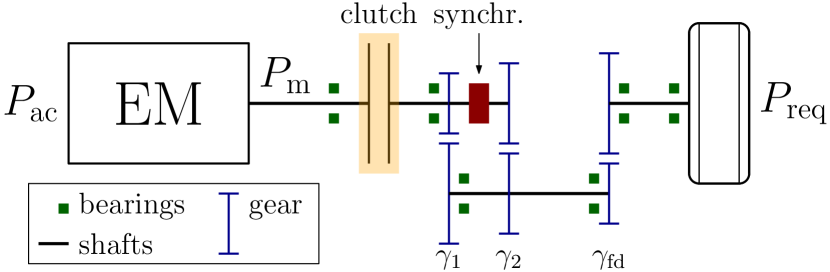
Figure 1: A schematic layout of the powertrain, including an EM and a two-gear transmission. This configuration consists of three shafts, six bearings, three gear pairs, a synchronizer (synchr.), and a clutch.

Related literature: This research relates to three general research streams. The first stream deals with (hybrid-) electric vehicle powertrain control and design optimization from a system perspective. This is also known as powertrain co-design, and it is typically solved with convex optimization (Pourabdollah et al., 2018; Borsboom et al., 2021) or derivative-free solvers (Ebbesen et al., 2012; Hegazy and van Mierlo, 2010). To ensure computational tractability, these methods either assume a fixed transmission efficiency or disregard losses entirely.

The second stream relates to the transmission design and control optimization at the component level (Qin et al., 2018; Lei et al., 2020; Patil et al., 2020). However, the optimization problems usually have component-specific objectives, like minimizing the noise and volume or maximizing the strength of the gear teeth, leveraging computationally-expensive finite-element models. Both the objectives and the methodologies do not connect well to the holistic, system-level perspective that is necessary in powertrain design optimization.

The third and final research stream pertains to more detailed transmission models in powertrain design, striking a balance between accurate modeling and system level design (Machado et al., 2021). The works in Hofstetter et al. (2018); Anselma et al. (2019) minimize the losses, but merely for one configuration. The procedure in Krüger et al. (2022) considers multiple topologies but provides no global optimality guarantees, whereas optimality is guaranteed in Leise et al. (2019), but fixed efficiencies for all transmission components are considered.

To conclude, to the best of the authors’ knowledge, there are no methods that can model and predict the losses of different transmission configurations in a modular and flexible fashion, in the context of a full electric powertrain, optimizing the design and control, whilst guaranteeing global optimality of the solution.

Statement of contributions: To address this issue, this paper presents a modular design and control optimization framework of electric vehicle transmissions. Specifically, we first derive detailed analytical loss models of all components that compose a transmission: the gears, the shafts, the bearings, the clutches and the synchronizers. Second, using engineering rules and manufacturer data, we methodically design a transmission system for a powertrain by combining the individual component models in the desired configuration. Third, we model the full drivetrain and the car, and pose an optimization problem to minimize the energy consumption over a drive cycle. Finally, we showcase our framework by optimizing the design of the two-gear transmission (2GT) of Fig. 1 and an FGT for a compact family electric car.

Organization: This paper is organized as follows: Section 2 presents the transmission component and shifting loss models, the systematic design approach, and the surrounding optimal design and control problem . We showcase our optimization framework with numerical results in Section 3. Finally, we draw the conclusions in Section 4, together with an outlook to future research.

2 Methodology

In this section, we construct the optimization problem, starting with the objective. Subsequently, we develop a model of the car and the powertrain, whereby we extensively elaborate on the gearbox and its components. To increase readability, some equations are purposely omitted from the main text. However, the interested reader can find these in the Appendix. Moreover, to keep our derivations concise, we will abandon the time dependency $t$, when its obvious from the context. Finally, we summarize the problem and present the solving method.

2.1 Objective and Longitudinal Vehicle Dynamics

The objective of the optimization is to minimize the energy provided to the EM over a drive cycle:

$$\min{E_{\mathrm{{\scriptsize ac}}}},$$ (1)

where $E_{\mathrm{{\scriptsize ac}}}$ is the energy consumed at the (electrical) input of the EM. The car is modeled following a quasi-static approach (Guzzella and Sciarretta, 2007) in time domain. The power request at the wheels $P_{\mathrm{{\scriptsize req}}}$ equals

$$P_{\mathrm{{\scriptsize req}}}=\frac{1}{2}\rho_{\mathrm{{\scriptsize a}}}c_{\mathrm{{\scriptsize d}}}A_{\mathrm{{\scriptsize f}}}v^{3}+v(m_{\mathrm{{\scriptsize v}}}+m_{\mathrm{{\scriptsize gb}}})\left(g(c_{\mathrm{{\scriptsize r}}}\cos{\beta}+\sin{\beta})+a\right),$$ (2)

where $v$, $a$ and $\beta$ are the time-dependent velocity, acceleration, and road inclination, respectively, provided by the drive cycle, $\rho_{\mathrm{{\scriptsize a}}}$ is the air density, $c_{\mathrm{{\scriptsize d}}}$ is the drag coefficient, $A_{\mathrm{{\scriptsize f}}}$ is the frontal area of the car, $m_{\mathrm{{\scriptsize v}}}$ is the vehicle mass without the gearbox, $m_{\mathrm{{\scriptsize gb}}}$ is the gearbox mass, $g$ is the gravitational constant, and $c_{\mathrm{{\scriptsize r}}}$ is the rolling resistance coefficient.

2.2 Transmission

In this section, we systematically design a transmission and model the components that a transmission contains, including its losses in an analytical fashion: the spur gear pairs ($\mathrm{g}$), the shafts ($\mathrm{s}$), the bearings ($\mathrm{b}$), the clutches ($\mathrm{cl}$), and the synchronizers ($\mathrm{syn}$). Using these component models, we can construct multiple transmission configurations in a flexible and modular fashion, and evaluate different transmission types. In this paper, we focus on the FGT and the 2GT, both designed in two stages. We describe the modeling procedure for a 2GT, and we can construct an FGT model by eliminating a pair of gears, a clutch, and a synchronizer.

Primarily, we optimize the gear ratio values $\gamma_{j}$. These are bounded by

$$\gamma_{j}\in[\gamma_{\mathrm{min}},\gamma_{\mathrm{max}}],\quad j\in\{1,2,\mathrm{fd}\}$$ (3)

where $\gamma_{1}$ is the ratio of the first gear pair, $\gamma_{2}$ is the ratio of the second gear pair, $\gamma_{\mathrm{{\scriptsize fd}}}$ is the final drive ratio, and $\gamma_{\mathrm{min}}$ and $\gamma_{\mathrm{max}}$ are the minimum and maximum values of the ratios. We ensure that the gear ratios are ordered from a high to a low ratio with the following constraint:

$$\gamma_{1}>\gamma_{2}.$$ (4)

Furthermore, the number of gear teeth on the pinions (the driving gears) $N_{\mathrm{{\scriptsize t}}}\in\mathbb{N}$ has to be a natural number, as well as the number of teeth on the driven gears $\gamma_{j}N_{\mathrm{{\scriptsize t}}}$:

$$\gamma_{j}N_{\mathrm{{\scriptsize t}}}\in\mathbb{N},\quad j\in\{1,2,\mathrm{fd}\}.$$ (5)

We demand the car to be able to launch at the maximum road inclination angle $\beta_{\mathrm{{\scriptsize max}}}$ in the highest gear ratio $\gamma_{1}$, guaranteed by the constraint

$$\gamma_{\mathrm{{\scriptsize 1}}}\gamma_{\mathrm{{\scriptsize fd}}}\geq\frac{gr_{\mathrm{{\scriptsize w}}}m_{\mathrm{{\scriptsize v}}}(c_{\mathrm{{\scriptsize r}}}\cos{\beta_{\mathrm{{\scriptsize max}}}}+\sin{\beta_{\mathrm{{\scriptsize max}}}})}{T_{\mathrm{{\scriptsize m,max}}}},$$ (6)

which partially defines our design space, where $T_{\mathrm{{\scriptsize m,max}}}$ is the maximum output torque of the EM and $r_{\mathrm{{\scriptsize w}}}$ is the radius of the wheels.

2.2.1 Initial Design

We initialize the design of the gearbox according to the procedures in Maciejczyk and Zdziennicki (2011) and start with the shafts. In the configuration of the transmission (see Fig. 1, we consider three shafts ($N_{\mathrm{{\scriptsize s}}}=3$): the input shaft ($k=1$), the intermediate shaft ($k=2$), and the output shaft ($k=3$), which are all assumed to be short and therefore infinitely stiff, neglecting shaft torsion. The torque limit of the gearbox is then determined by the radius of the shafts. We determine the radius of a shaft $r_{\mathrm{s},k}$ using the following equation:

$$r_{\mathrm{s},k}=\sigma_{\mathrm{{\scriptsize s}}}T_{k,\mathrm{max}}^{\frac{1}{3}},\quad k\in\{1,2,3\}$$ (7)

where $T_{k,\mathrm{max}}$ is the maximum torque that shaft $k$ needs to cope with, defined by $T_{\mathrm{{\scriptsize m,max}}}$ and the gear ratio $\gamma_{j}$, and $\sigma_{\mathrm{{\scriptsize s}}}$ is a parameter defined in the Appendix.

The pinions of the first gear pair and final drive are designed as the shaft with teeth mounted on the circumference, which means that the root radius of these pinions is equal to the radius of the shaft. Their pitch radius $r_{\mathrm{p},j}$ is then determined using

$$r_{\mathrm{p},j}=\frac{r_{\mathrm{{\scriptsize s,1}}}}{1-\frac{\sigma_{\mathrm{{\scriptsize p}}}}{N_{\mathrm{{\scriptsize t}}}}},\quad j\in\{1,\mathrm{fd}\},\quad k\in\{1,2\},$$ (8)

where $\sigma_{\mathrm{{\scriptsize p}}}$ is a pitch radius parameter defined in the Appendix. In general, the radius of a driven gear $r_{\mathrm{g},j}$ is equal to

$$r_{\mathrm{g},j}=r_{\mathrm{p},j}\gamma_{j},\quad j\in\{1,2,\mathrm{fd}\}.$$ (9)

For every gear pair, except the final drive, the distance between the centers of the pinion and gear $d_{\mathrm{{\scriptsize g}}}$ has to be equal, since they must be mounted on the same shafts:

$$d_{\mathrm{{\scriptsize g}}}=r_{\mathrm{{\scriptsize p,1}}}+r_{\mathrm{{\scriptsize g,1}}}=r_{\mathrm{{\scriptsize p,2}}}+r_{\mathrm{{\scriptsize g,2}}}.$$ (10)

In our framework, we determine the value of $d_{\mathrm{{\scriptsize g}}}$ from the design of the first gear and comply with that distance in the second gear. Since the pitch radii of the first gear pair are now known, the pitch radius of the pinion for the remaining gear pair $r_{\mathrm{p},2}$ is equal to

$$r_{\mathrm{p},2}=d_{\mathrm{{\scriptsize g}}}\left(1-\frac{1}{1+\gamma_{2}}\right).$$ (11)

We calculate the outer radius of the clutch $r_{\mathrm{{\scriptsize cl,o}}}$ using the methods in (Ba̧k, 2021), namely

$$r_{\mathrm{{\scriptsize cl,o}}}=\sigma_{\mathrm{{\scriptsize cl,o}}}T_{\mathrm{{\scriptsize m,max}}}^{\frac{1}{3}},$$ (12)

where $\sigma_{\mathrm{{\scriptsize cl,o}}}$ is a clutch radius parameter defined in the Appendix. The inner radius of the clutch $r_{\mathrm{cl,i}}$ then becomes

$$r_{\mathrm{{\scriptsize cl,i}}}=\phi_{\mathrm{{\scriptsize cl}}}r_{\mathrm{{\scriptsize cl,o}}},$$ (13)

where $\phi_{\mathrm{{\scriptsize cl}}}$ is the predefined ratio between the outer and inner radius of the clutch. The force required to engage the clutch plates $F_{\mathrm{{\scriptsize cl}}}$ is equal to

$$F_{\mathrm{{\scriptsize cl}}}=\sigma_{\mathrm{{\scriptsize cl}}}\left(r_{\mathrm{{\scriptsize cl,o}}}^{2}-r_{\mathrm{{\scriptsize cl,i}}}^{2}\right),$$ (14)

where $\sigma_{\mathrm{{\scriptsize cl}}}$ is a clutch force parameter defined in the Appendix.

Since the size of the rotating part of a bearing is small, we neglect its inertia and we consider its mass $m_{\mathrm{{\scriptsize b}}}$ to be constant. The latter can be found in manufacturer catalogues, including its width $b_{\mathrm{{\scriptsize b}}}$ (SKF Group, 2018). The inertia and mass of all remaining modeled gearbox components are approximated by assuming all components are thick-walled cylindrical tubes with open ends. Therefore, the mass of a component $m_{c}$ can be calculated using

$$m_{c}=\rho_{c}b_{c}\pi(r_{c,\mathrm{o}}^{2}-r_{c,\mathrm{i}}^{2}),\quad c\in\{\mathrm{g},\mathrm{s},\mathrm{cl},\mathrm{syn}\},$$ (15)

where $\rho_{c}$ is the density of the material of the component, $b_{c}$ is the width ($c\in\{\mathrm{g},\mathrm{cl},\mathrm{syn}$}), or length ($c=\mathrm{s)}$ of the component, and $r_{c,\mathrm{o}}$ and $r_{c,\mathrm{i}}$ are the outer and inner radius, respectively. In our case, $r_{\mathrm{{\scriptsize s,i}}}=0$ and $r_{\mathrm{{\scriptsize g,i}}}=r_{\mathrm{{\scriptsize syn,i}}}=r_{\mathrm{{\scriptsize s,o}}}$, since we consider the gears and synchronizers to be directly mounted on the shafts. We assume $b_{\mathrm{{\scriptsize g}}}$ is related to the gear radius (see Appendix), which is equal to $b_{\mathrm{{\scriptsize syn}}}$. The length of a shaft $b_{\mathrm{{\scriptsize s}}}$ is the summation of the width of all the components mounted on it. This makes the inertia $J_{c}$ equal to

$$J_{c}=\frac{1}{2}m_{c}(r_{c,\mathrm{o}}^{2}+r_{c,\mathrm{i}}^{2}),\quad c\in\{\mathrm{g},\mathrm{s},\mathrm{cl},\mathrm{syn}\}.$$ (16)

For the complete gearbox, the mass $m_{\mathrm{{\scriptsize gb}}}$ and inertia $J_{\mathrm{{\scriptsize gb}}}$ are equal to the summation of all the masses and inertias of the components, respectively.

2.2.2 Gear losses

The gear losses are split into four types: The sliding ($\mathrm{sl}$) and roll ($\mathrm{r}$) friction, and the oil churning ($\mathrm{ch}$) and windage ($\mathrm{wi}$) losses. The sliding and roll friction losses are modeled using the elasto-hydrodynamic lubrication (EHL) model (Xu et al., 2007). The sliding friction loss is equal to

$$F_{\mathrm{{\scriptsize g,sl}}}=\mu W,$$ (17)

where $\mu$ is the sliding coefficient fully defined in the Appendix and $W$ is the normal force on the tooth. By calculating the sliding coefficient for a slide-to-roll ratio for a gear mesh cycle, the average sliding friction during rotation can be determined.

The expression of the rolling friction loss $F_{\mathrm{{\scriptsize g,r}}}$ is given in the Appendix.

As the gears are only partially submerged in lubrication oil, there are both oil churning losses (dragging through the oil) and windage losses (moving through the air). We use the same model for approximating both these types of losses, but with different material properties, expressed in three terms (Seetharaman, 2009): The losses at the circumference $P_{\mathrm{{\scriptsize ch,p}}}$, the faces $P_{\mathrm{{\scriptsize ch,f}}}$, and teeth cavities $P_{\mathrm{{\scriptsize ch,c}}}$. The full expressions of these models are given in the Appendix.

The total power lost due to oil churning $P_{\mathrm{{\scriptsize g,ch}}}$ is then equal to

$$P_{\mathrm{{\scriptsize g,ch}}}=P_{\mathrm{{\scriptsize ch,p}}}+P_{\mathrm{{\scriptsize ch,f}}}+P_{\mathrm{{\scriptsize ch,c}}},$$ (18)

using the parameters for oil, and the windage power loss can be expressed as

$$P_{\mathrm{{\scriptsize g,wi}}}=P_{\mathrm{{\scriptsize ch,p}}}+P_{\mathrm{{\scriptsize ch,f}}},$$ (19)

using the parameters for air. We do not include the teeth cavity losses in the windage model, since these losses are negligible according to Seetharaman (2009). The total power loss caused by the gears $P_{\mathrm{{\scriptsize g}}}$ is summed as

$$P_{\mathrm{{\scriptsize g}}}=(F_{\mathrm{{\scriptsize g,sl}}}+F_{\mathrm{{\scriptsize g,r}}})v_{\mathrm{{\scriptsize e}}}+P_{\mathrm{{\scriptsize g,ch}}}+P_{\mathrm{{\scriptsize g,wi}}},$$ (20)

where $v_{\mathrm{{\scriptsize e}}}$ is the speed of the contact surface.

2.2.3 Bearings

The bearings are modeled by dividing the losses into four terms: The moments of rolling ($\mathrm{r}$), sliding ($\mathrm{sl}$), seal ($\mathrm{s}$), and drag friction ($\mathrm{drag}$) (SKF Group, 2008). The bearing rolling and sliding frictional moments are similar to the gear counterparts. We disregard the seal frictional moment, since we assume that the gearbox is a closed system and does not require sealing. The drag friction is a combination of the remaining losses, i.e., oil churning and windage.

The rolling frictional moment $T_{\mathrm{{\scriptsize b,r}}}$ is equal to

$$T_{\mathrm{{\scriptsize b,r}}}=\sigma_{\mathrm{{\scriptsize b,r}}}\omega_{\mathrm{{\scriptsize b}}}^{0.6}$$ (21)

where $\sigma_{\mathrm{{\scriptsize b,r}}}$ is a bearing roll parameter defined in the Appendix and $\omega_{\mathrm{{\scriptsize b}}}$ is the rotational speed of the bearing.

The sliding frictional moment $T_{\mathrm{{\scriptsize b,sl}}}$ is represented by

$$T_{\mathrm{{\scriptsize b,sl}}}=G_{\mathrm{{\scriptsize sl}}}(\phi_{\mathrm{{\scriptsize bl}}}\mu_{\mathrm{{\scriptsize bl}}}+(1-\phi_{\mathrm{{\scriptsize bl}}})\mu_{\mathrm{{\scriptsize EHL}}}),$$ (22)

where $G_{\mathrm{{\scriptsize sl}}}$ is a bearing and load-dependent variable, $\phi_{\mathrm{{\scriptsize bl}}}$ is a weighting factor, $\mu_{\mathrm{{\scriptsize bl}}}$ is a constant depending on movement (stationary or rotating), and $\mu_{\mathrm{{\scriptsize EHL}}}$ is the sliding friction in full-film EHL conditions.

The drag frictional moment $T_{\mathrm{{\scriptsize b,drag}}}$ is calculated using

$$T_{\mathrm{{\scriptsize b,drag}}}=\sigma_{\mathrm{{\scriptsize b,drag}}}\omega_{\mathrm{{\scriptsize b}}}^{2}+\bar{\sigma}_{\mathrm{{\scriptsize b,drag}}}\omega_{\mathrm{{\scriptsize b}}}^{\epsilon_{\mathrm{{\scriptsize b,drag}}}},$$ (23)

where $\sigma_{\mathrm{{\scriptsize b,drag}}}$, $\bar{\sigma}_{\mathrm{{\scriptsize b,drag}}}$, and $\epsilon_{\mathrm{{\scriptsize b,drag}}}$ are all bearing drag parameters defined in the Appendix.

To summarize, the total bearing power loss $P_{\mathrm{{\scriptsize b}}}$ is equal to

$$P_{\mathrm{{\scriptsize b}}}=(T_{\mathrm{{\scriptsize b,r}}}+T_{\mathrm{{\scriptsize b,s}}}+T_{\mathrm{{\scriptsize b,drag}}})\omega_{\mathrm{{\scriptsize b}}},$$ (24)

whereby we assume to have two bearings per shaft in our configuration.

2.2.4 Shafts

Depending on the location of the shaft in the transmission system, it is possibly (partially) submerged by oil. Therefore we can model the losses incurred by the shafts $P_{\mathrm{{\scriptsize s}}}$ in one term, namely oil churning. The expression is equal to the one used for the churning of the gears, and is given in (18).

2.2.5 Clutches

We equip the powertrain with a dry clutch, which leaves us with windage losses as the mere loss term for the clutch losses $P_{\mathrm{{\scriptsize cl}}}$. Its model is identical to (19).

2.2.6 Synchronizers

The oil layer between the synchronizers and the gears causes a drag power when there is a difference in velocity between the synchronizer and gear, i.e., when a gear pair is disconnected. This drag power $P_{\mathrm{{\scriptsize syn}}}$ is equal to (Dogan, 2001)

$$P_{\mathrm{{\scriptsize syn}}}=\sigma_{\mathrm{{\scriptsize syn}}}(\omega_{\mathrm{{\scriptsize syn}}}-\omega_{\mathrm{{\scriptsize g}}})\omega_{\mathrm{{\scriptsize syn}}},$$ (25)

where $\sigma_{\mathrm{{\scriptsize syn}}}$ is a synchronizer drag parameter defined in the Appendix, $\omega_{\mathrm{{\scriptsize syn}}}$ is the speed of the synchronizer (equal to the speed of the previously selected gear), and $\omega_{\mathrm{{\scriptsize g}}}$ is the speed of the currently selected gear.

2.2.7 Full Gearbox Model

As mentioned previously, we model the powertrain using the quasi-static (backward-facing) modeling approach, to make fair comparisons between configurations. However, all transmission loss models introduced so far are forward-facing. We overcome this issue by first establishing a loss map for the operating range of each gear in the transmission, and subsequently simulating the drive cycle in a quasi-static fashion and interpolating the losses in the simulation. We minimize the interpolation errors by creating the loss maps with a fine grid. The combined power losses $P_{\mathrm{{\scriptsize gb,loss}}}$ are equal to

$$P_{\mathrm{{\scriptsize gb,loss}}}=P_{\mathrm{{\scriptsize g,fd}}}+\sum_{k=1}^{N_{\mathrm{{\scriptsize s}}}}\left(2P_{\mathrm{b},k}+P_{\mathrm{s},k}\right)+J\frac{va}{r_{\mathrm{{\scriptsize w}}}^{2}}\\ \begin{cases}+P_{\mathrm{{\scriptsize g,1}}}&\text{ if }N_{\mathrm{{\scriptsize g}}}=1\\ +P_{\mathrm{{\scriptsize g,1}}}+P_{\mathrm{{\scriptsize g,2}}}+P_{\mathrm{{\scriptsize cl}}}+P_{\mathrm{{\scriptsize syn}}}&\text{ if }N_{\mathrm{{\scriptsize g}}}=2,\end{cases}$$ (26)

where $J$ is the inertia of the complete drivetrain including the wheels.

2.2.8 Shifting

We model the actuators that engage the clutch and synchronizers during shifting with a fixed efficiency $\eta_{\mathrm{a},c}$. The energy consumed by an actuator $E_{\mathrm{a},c}$ is then equal to

$$E_{\mathrm{a},c}=\frac{2F_{\mathrm{a},c}h_{\mathrm{a},c}}{\eta_{\mathrm{a},c}},\quad c\in\{\mathrm{cl},\mathrm{syn}\}$$ (27)

where $F_{\mathrm{a},c}$ is the force needed by the actuator to move the clutch or synchronizer, and $h_{\mathrm{a},c}$ is the distance over which the clutch or synchronizer is moved. Specifically, the actuation distance of a synchronizer is assumed to be related to its width, $h_{\mathrm{a,syn}}=\frac{b_{\mathrm{{\scriptsize syn}}}}{2}$.

The synchronization of the clutch plates is approximated through the slip speed $\omega_{\mathrm{{\scriptsize sl}}}(t)$, which is equal to (Park and Choi, 2021)

$$\omega_{\mathrm{{\scriptsize sl}}}(t)=\mathit{\Delta}\omega_{\mathrm{{\scriptsize cl,0}}}e^{-\zeta t},$$ (28)

where $\mathit{\Delta}\omega_{\mathrm{{\scriptsize cl,0}}}$ is the initial relative angular velocity between the two clutch plates, i.e. between the EM speed and the speed of the wheels through the currently selected gear, $\zeta$ is the rate at which the pressure in the clutch increases — and therefore dependent on the clutch springs and actuator —, and $t$ is the time. We match the speeds up to a tolerance equal to $\omega_{\mathrm{{\scriptsize sl}}}\leq$ 1 rad/s. The energy lost during this shifting phase $E_{\mathrm{{\scriptsize sh}}}$, including the inertial losses, is equal to

$$\mathit{\Delta}E_{\mathrm{{\scriptsize sh}}}=\int_{0}^{t_{\mathrm{{\scriptsize sh}}}}\left((J_{1}+J_{2})T_{\mathrm{{\scriptsize m}}}+J_{1}J_{2}\zeta\omega_{\mathrm{{\scriptsize sl}}}(t)\right)\frac{\omega_{\mathrm{{\scriptsize sl}}}(t)}{J_{1}+J_{2}}\mathrm{d}t\\ +E_{\mathrm{{\scriptsize a,cl}}}+E_{\mathrm{{\scriptsize a,syn}}},$$ (29)

where $t_{\mathrm{{\scriptsize sh}}}$ is the duration of a gear shift, $J_{1}$ is the inertia of the components between the EM and first clutch plate, and $J_{2}$ is the inertia of the components between the second clutch plate and the wheels.

2.3 Electric Motor

For any negative power requests, the EM power output is saturated to the maximum EM power $P_{\mathrm{{\scriptsize m,max}}}$. The EM power output $P_{\mathrm{{\scriptsize m}}}$ then equals

$$P_{\mathrm{{\scriptsize m}}}=\begin{cases}P_{\mathrm{{\scriptsize req}}}+P_{\mathrm{{\scriptsize gb,loss}}}&\text{ if }P_{\mathrm{{\scriptsize req}}}\geq 0\\ \max{\left(-P_{\mathrm{{\scriptsize m,max}}},r_{\mathrm{{\scriptsize b}}}P_{\mathrm{{\scriptsize req}}}+P_{\mathrm{{\scriptsize gb,loss}}}\right)}&\text{ if }P_{\mathrm{{\scriptsize req}}}<0,\end{cases}$$ (30)

where $r_{\mathrm{{\scriptsize b}}}$ is the regenerative braking fraction. The speed of the EM $\omega_{\mathrm{{\scriptsize m}}}$ is equal to

$$\omega_{\mathrm{{\scriptsize m}}}=\gamma_{j}\gamma_{\mathrm{{\scriptsize fd}}}\frac{v}{r_{\mathrm{{\scriptsize w}}}},\quad j\in\{1,2\},$$ (31)

which is equivalent to the input speed of the gearbox, where $j$ is the selected gear. We model the EM using a quasi-static efficiency map:

$$P_{\mathrm{{\scriptsize ac}}}=\begin{cases}\frac{P_{\mathrm{{\scriptsize m}}}}{\eta_{\mathrm{{\scriptsize m}}}(P_{\mathrm{{\scriptsize m}}},\omega_{\mathrm{{\scriptsize m}}})}&\text{ if }P_{\mathrm{{\scriptsize m}}}\geq 0\\ \eta_{\mathrm{{\scriptsize m}}}(P_{\mathrm{{\scriptsize m}}},\omega_{\mathrm{{\scriptsize m}}})P_{\mathrm{{\scriptsize m}}}&\text{ if }P_{\mathrm{{\scriptsize m}}}<0.\end{cases}$$ (32)

2.4 Optimization Problem

In this section, we summarize the optimal design and control problem of the 2GT. Due to space limitations, we omit the FGT problem, considering it is a simplified, design-only instance of the 2GT problem. The state variables are $x=(E_{\mathrm{{\scriptsize ac}}},i)$, where $i\in\{1,2\}$ is the current gear. The design variables are $p=\gamma_{j}$ where $j\in\{1,2,\mathrm{fd}\}$. Finally, the control variable is $u\in\mathcal{U}(i)$, which is equal to the shift input: $\mathcal{U}(1)\in\{0,1\}$ (only an upshift or no shifting is possible), otherwise, $\mathcal{U}(2)\in\{-1,0\}$ (merely a downshift or no shifting). The design problem of an FGT is identical, with simplifications in the sense that $i=1$, $j\in\{1,\mathrm{fd}\}$, and no control input is present.

Problem 1 (Optimal Co-Design Problem)

The 2GT minimum energy design and control are the solution of

$$\!\min_{u,p} E_{\mathrm{{\scriptsize ac}}}(p,u)=\int_{0}^{t_{\mathrm{{\scriptsize f}}}}P_{\mathrm{{\scriptsize ac}}}\mathrm{d}t+\mathit{\Delta}E_{\mathrm{{\scriptsize sh}}}(u)$$

s.t. $$i_{\mathrm{{\scriptsize next}}}=i_{\mathrm{{\scriptsize current}}}+u$$

$$\eqref{eq:wheels}-\eqref{eq:em_effmap}.$$

We reformulate this problem to an equivalent nested co-design problem, which is visualized in Fig. 2 (Fathy, 2003).

Figure 2: A visualization of the nested solution strategy of the 2GT design and control optimization problem.

Problem 2 (Nested Co-Design Problem)

The 2GT minimum energy design and control are the solution of the nested problem

$$\!\min_{p} E_{\mathrm{{\scriptsize ac}}}(p,u^{\star}(p))=\int_{0}^{t_{\mathrm{{\scriptsize f}}}}P_{\mathrm{{\scriptsize ac}}}\mathrm{d}t+\mathit{\Delta}E_{\mathrm{{\scriptsize sh}}}(u^{\star}(p))$$

s.t. $$u^{\star}(p)=\mathop{\mathrm{argmin}}_{u}E_{\mathrm{{\scriptsize ac}}}(p,u)$$

$$\eqref{eq:wheels}-\eqref{eq:em_effmap}.$$

2.5 Discussion

A few comments are in order. First of all, a number of assumptions, approximations, and generalizations are made in the configuration, the design process, and component selection. Although these assumptions are based on industrial standards and examples, our framework can be modified to other desired initial designs and configurations. Second, we do not incorporate dynamic thermal effects, since gearbox temperatures are generally constant in steady-state conditions and do not affect the design. Third, we also do not consider volumetric constraints, yet these can be taken into consideration when data is available of the specific car. Moreover, this framework serves as an instrument for gear ratio selection in initial stages of powertrain design, where packaging issues can be addressed in later phases. Finally, we only consider two ratio stages — first (and second) gear and the final drive — in a spur-gear fashion. Usually, a drivetrain also contains a differential, and can contain other types of gearing, like planetary gear sets or helical gears, etc. This can be implemented in our framework with additional modeling, which will be left to a future extension of this paper.

3 Results

In this section, we present the numerical results of applying the systematic modeling methods and the co-design optimization framework presented in Section 2 to optimize the design of an FGT and the control and design of a 2GT in a compact family electric vehicle. We select the vehicle and baseline powertrain parameter values of a Nissan Leaf, shown in Table 1 (Carinf, 2022), and the Common Artemis Drive Cycle (CADC) as the driving mission, since it is a relatively challenging cycle. The most relevant gearbox modeling parameter values are given in Table 2, while the more specific parameters are defined in Table 4 in the Appendix. We discretize the problem using the Euler Forward method, with a sampling time of 1 s. Since the optimization problem is highly non-linear, we solve the design problem in the outer layer with an exhaustive search, while the control problem in the inner layer is solved using dynamic programming. In other words, both of these layers are solved using methods offering global optimality guarantees, providing us with a solution with the same properties. Since the number of teeth on any gear must be a natural number, we discretize the design space with gear step size $\Delta\gamma_{j}=\frac{1}{N_{\mathrm{{\scriptsize t}}}}$. The design space is further reduced by only considering designs that can attain the maximum speed and acceleration requested by the CADC, $v_{\mathrm{{\scriptsize max}}}$ and $a_{\mathrm{{\scriptsize max}}}$, respectively, and the road inclination demand of $\beta_{\mathrm{{\scriptsize max}}}$. This leaves us with 355 feasible designs for the FGT, and 65820 for the 2GT. All computations were performed on an AMD Ryzen 5 5600x CPU and NVIDIA GeForce RTX 3070 Ti GPU, resulting in computation times of around 40 s for the FGT and around 7 h for the 2GT.

Table 1: Vehicle & EM Parameters

Symbol	Variable	Value	Unit
Vehicle
$A_{\mathrm{{\scriptsize f}}}$	Frontal Area	2.27	[m2]
$c_{\mathrm{{\scriptsize d}}}$	Drag coefficient	0.29	[1]
$c_{\mathrm{{\scriptsize r}}}$	Rolling resistance coefficient	0.01	[1]
$g$	Gravitational constant	9.81	[N/kg]
$\rho_{a}$	Air density	1.225	[kg/m3]
$m_{\mathrm{{\scriptsize v}}}$	Vehicle mass without gearbox	1513	[kg]
$m_{\mathrm{{\scriptsize w}}}$	Wheel mass	20	[kg]
$r_{\mathrm{{\scriptsize w}}}$	Wheel radius	0.327	[m]
$r_{\mathrm{{\scriptsize b}}}$	Regenerative brake fraction	0.55	[1]
Electric Motor
$T_{\mathrm{{\scriptsize m,max}}}$	Maximum EM output torque	287	[Nm]
$\omega_{\mathrm{{\scriptsize m,max}}}$	Maximum EM speed	10,000	[rpm]

Table 2: Gearbox Parameters

Symbol	Variable	Value	Unit
$N_{\mathrm{{\scriptsize t}}}$	Number of teeth on a pinion	17	[1]
$\rho_{c}$	Density of steel	7,850	[kg/m3]
$\beta_{\mathrm{{\scriptsize max}}}$	Maximum road inclination	7.5	[∘]
$\gamma_{\mathrm{{\scriptsize min}}}$	Minimum gear stage ratio	1	[1]
$\gamma_{\mathrm{{\scriptsize max}}}$	Maximum gear stage ratio	5	[1]
$b_{\mathrm{{\scriptsize cl}}}$	Clutch width	16	[mm]
$b_{\mathrm{{\scriptsize s,3}}}$	Output shaft length	1.536	[m]
$t_{\mathrm{{\scriptsize sh}}}$	Shifting time	0.5	[s]
$h_{\mathrm{{\scriptsize a,cl}}}$	Clutch actuation distance	4	[mm]
$F_{\mathrm{{\scriptsize a,syn}}}$	Synchronizer actuation force	300	[N]
$\eta_{\mathrm{a},c}$	Actuator efficiency	0.8	[1]
$\phi_{\mathrm{{\scriptsize cl}}}$	Clutch radius ratio	0.7	[1]

3.1 Numerical Results

The solutions are summarized in Table 3. We solve the FGT design problem for two cases: with and without a road inclination constraint. The obtained solutions are shown in Fig. 4, where they are framed within the objective values of the full design space. The test case with a road inclination constraint $\beta_{\mathrm{{\scriptsize max}}}=7.5^{\circ}$ results in a design of $\gamma_{1}\approx 3.2$, $\gamma_{\mathrm{{\scriptsize fd}}}\approx 2.2$. The subsequent efficiency maps of both gear stages combined, and the EM are shown in Fig. 3, together with the interrelated operating points over the CADC. The total energy consumption at the end of the cycle is equal to $E_{\mathrm{{\scriptsize ac}}}(t_{\mathrm{{\scriptsize f}}})=$ 8.30 kWh. When we ignore the gradeability constraint, we obtain a design of $\gamma_{1}\approx 2.7$, $\gamma_{\mathrm{{\scriptsize fd}}}\approx 1.8$, and $E_{\mathrm{{\scriptsize ac}}}(t_{\mathrm{{\scriptsize f}}})=$ 8.12 kWh; a difference of 2.2 %. However, the maximum road inclination the vehicle can handle with this gearbox design is only $5^{\circ}$.

If we solve the 2GT design and control problem for the same vehicle, we arrive at the solutions shown in Fig. 5 and Table 3. This is a design of $\gamma_{1}\approx 2.82$, $\gamma_{2}\approx 1.18$, $\gamma_{\mathrm{{\scriptsize fd}}}\approx 2.59$, and $E_{\mathrm{{\scriptsize ac}}}(t_{\mathrm{{\scriptsize f}}})=$ 8.23 kWh; an energy consumption decrease of 0.8 % with respect to the FGT solution with the gradeability constraint, since both the transmission and EM are allowed to operate in more efficient regions. We observe a reasonable shifting trajectory, where the second gear is selected only in higher-speed regions.

Table 3: Transmission Design Solutions

Configuration	${\gamma_{1}}$	${\gamma_{2}}$	${\gamma_{\mathrm{{\scriptsize fd}}}}$	${E_{\mathrm{{\scriptsize ac}}}(t_{\mathrm{{\scriptsize f}}})}$
FGT (Baseline)	$\frac{31}{17}$	-	$\frac{74}{17}$	8.48 kWh
FGT (Gradeab. constr.)	$\frac{55}{17}$	-	$\frac{38}{17}$	8.30 kWh
FGT (No gradeab. constr.)	$\frac{46}{17}$	-	$\frac{31}{17}$	8.12 kWh
2GT (Optimized)	$\frac{48}{17}$	$\frac{20}{17}$	$\frac{44}{17}$	8.23 kWh

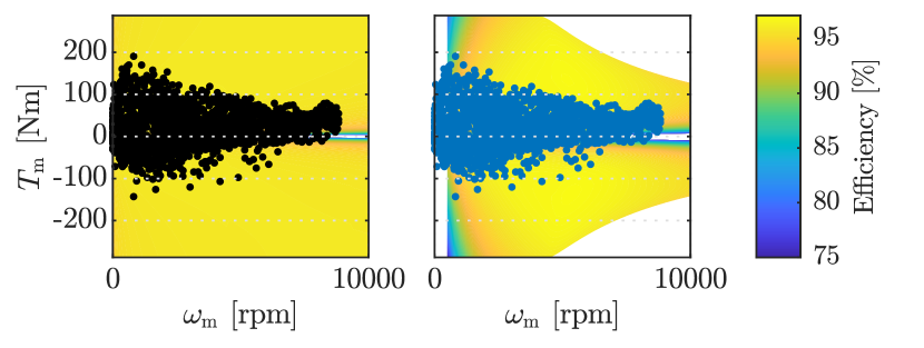
Figure 3: The efficiency maps of the optimally-designed FGT (left) and the EM (right) with the gradeability constraint, including the operating points over the CADC.

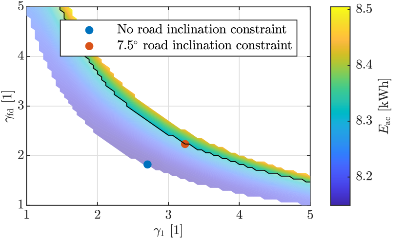
Figure 4: The optima and sensitivity of the optimal control solutions in the feasible design set of the FGT, excluding the gradeabilty constraint (the full set) and including it (the set above the black boundary).

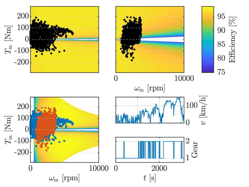
Figure 5: The efficiency maps of the optimally designed 2GT (first gear: top left, second gear: top right) and the EM (bottom left), including the operating points, and the shifting trajectory.

3.2 Validation

Whilst validation of our methods using high-fidelity models is subject to future research, we can examine whether our simulation results are in the appropriate range of values. We compare our simulations and optimal solutions to the baseline design of the 2012 Nissan Leaf, which is equipped with an FGT of $\gamma_{1}\approx 1.88$ and $\gamma_{\mathrm{{\scriptsize fd}}}\approx 4.24$ (Nelson, 2020). We recreate the transmission with our methodology, and resimulate the vehicle on the CADC (Table 3) and the New European Driving Cycle (NEDC), since OEM performance data is reported on the latter. To make an estimation on the battery energy consumption, the battery and inverter are both modeled using a fixed efficiency, equal to 97.5 % (Steilen and Jörissen, 2015; HomerEnergy, 2022) and 95 % (Chang et al., 2019), respectively. This amounts to a simulated energy consumption over the NEDC of 1.37 kWh, which equates to 125.7 Wh/km. OEM data reports an energy consumption of 126 Wh/km: an error of 0.2 %, which leads to the affirmation that our models and methods are sufficiently accurate for this purpose.

4 Conclusions

In this paper, we aimed at bridging the gap in transmission modeling, between simple models in powertrain sizing and high-fidelity models for component design optimization, in order to rapidly explore the extensive powertrain design space. To this end, we instantiated a modeling and optimization framework that can simulate different types of transmissions by systematically constructing a configuration, analytically modeling the individual components that it contains, and optimizing the shifting control. We showcased our framework for a compact family electric car, where the FGT optimum we obtain is slightly different from the baseline design, mainly due to packaging constraints of the final drive within the differential. Implementing a 2GT can improve the energy consumption, but it might come at the price of higher complexity, volume, mass, and cost. We validated our framework, showing only a slight deviation in energy consumption when the real-world configuration is modeled, proving that our framework can be used for gear ratio selection, from which expert engineers can further improve the detailed design of the gearbox.

This study introduces the following paths for future research: First of all, as mentioned previously, our framework could be validated more extensively with high-fidelity models. Second, the impact of a higher number of gears, possibly combined with more challenging performance requirements, can be readily explored with our framework. Finally, we can combine our transmission framework with EM and battery sizing, to holistically design an electric vehicle powertrain.

We thank Dr. Ilse New and Ir. Fabio Paparella for proofreading this paper.

Appendix A Detailed Gearbox Modeling

In this appendix, we introduce the more detailed gearbox component models. Material and type-specific values of the parameters can be found in Table 4, or in the individual sources cited at the introduction of the models.

The width of a gear $b_{\mathrm{{\scriptsize g}}}$ is related to its radius through

$$b_{\mathrm{{\scriptsize g}}}=16\frac{2r_{\mathrm{{\scriptsize g}}}}{N_{\mathrm{{\scriptsize t}}}}.$$ (33)

The parameter $\sigma_{\mathrm{{\scriptsize s}}}$ used to determine the radius of the shaft $r_{\mathrm{{\scriptsize s}}}$ is equal to

$$\sigma_{\mathrm{{\scriptsize s}}}=2\cdot 10^{-2}\left(\frac{2}{5\pi}\right)^{\frac{1}{3}}.$$ (34)

The parameter $\sigma_{\mathrm{{\scriptsize cl,o}}}$ used to determine the outer radius of the clutch $r_{\mathrm{{\scriptsize cl,o}}}$ is equal to

$$\sigma_{\mathrm{{\scriptsize cl,o}}}=\left(\frac{3}{2\pi p_{\mathrm{{\scriptsize cl}}}(N_{\mathrm{{\scriptsize z}}}\mu_{\mathrm{{\scriptsize cl}}})^{2}(1-\gamma_{\mathrm{{\scriptsize cl}}}^{3})}\right)^{\frac{1}{3}},$$ (35)

where $p_{\mathrm{{\scriptsize cl}}}$ is the maximum clutch plate surface pressure, $N_{\mathrm{{\scriptsize z}}}$ is the number of clutch plates, and $\mu_{\mathrm{{\scriptsize cl}}}$ is the friction coefficient of the clutch surface (Ba̧k, 2021). The parameter $\sigma_{\mathrm{{\scriptsize cl}}}$ used to calculate the force required to engage the clutch plate is equal to

$$\sigma_{\mathrm{{\scriptsize cl}}}=\pi N_{\mathrm{{\scriptsize z}}}\mu_{\mathrm{{\scriptsize cl}}}p_{\mathrm{{\scriptsize cl}}}.$$ (36)

The full expression of the gear sliding losses $F_{\mathrm{{\scriptsize g,sl}}}$, as a function of the slide-to-roll ratio $S$, is given by

$$F_{\mathrm{{\scriptsize g,sl}}}=e^{f}p^{b_{\mathrm{{\scriptsize 2}}}}_{\mathrm{{\scriptsize h}}}|S|^{b_{\mathrm{{\scriptsize 3}}}}v^{b_{\mathrm{{\scriptsize 6}}}}_{\mathrm{{\scriptsize e}}}\nu^{b_{\mathrm{{\scriptsize 7}}}}R^{b_{\mathrm{{\scriptsize 8}}}}W,$$ (37a)

$$f=b_{\mathrm{{\scriptsize 1}}}+b_{\mathrm{{\scriptsize 4}}}|S|p_{\mathrm{{\scriptsize h}}}\log(\nu)+b_{\mathrm{{\scriptsize 5}}}e^{-|S|p_{\mathrm{{\scriptsize h}}}\log(\nu)}+b_{\mathrm{{\scriptsize 9}}}e^{s},$$ (37b)

where $p_{\mathrm{{\scriptsize h}}}$ is the Hertzian pressure at the contact surface, $\nu$ is the dynamic viscosity of the oil calculated using the Walther equation (Seeton, 2006), $s$ is the surface roughness of the gears, $R$ is the effective radius of curvature, and $b_{\mathrm{{\scriptsize 1}}},...,b_{\mathrm{{\scriptsize 9}}}$ are coefficients determined by the oil (Xu et al., 2007).

The rolling friction loss is equal to

$$F_{\mathrm{{\scriptsize g,r}}}=4.318(\tilde{G}\tilde{U})^{0.658}\tilde{Q}^{0.0126}\frac{R}{\alpha},$$ (38)

where $\tilde{G}$ is a material parameter, $\tilde{U}$ is a speed parameter, $\tilde{Q}$ is a load parameter, and $\alpha$ is the pressure viscosity coefficient of the oil (Xu et al., 2007).

The three churning models are equal to

$$P_{\mathrm{{\scriptsize ch,p}}}=4\nu b_{\mathrm{{\scriptsize g}}}r_{\mathrm{{\scriptsize g,o}}}^{2}\omega_{\mathrm{{\scriptsize g}}}^{2}\cos^{-1}{(1-\tilde{h})}$$ (39a)

$$P_{\mathrm{{\scriptsize ch,f}}}=\left(b_{\mathrm{{\scriptsize 10}}}\theta_{\mathrm{{\scriptsize oil}}}\nu^{b_{\mathrm{{\scriptsize 11}}}}\omega_{\mathrm{{\scriptsize g}}}^{b_{\mathrm{{\scriptsize 12}}}}r_{\mathrm{{\scriptsize g,o}}}^{b_{\mathrm{{\scriptsize 13}}}}\right)\\ \frac{\Big{(}\frac{\pi}{2}{-\sin^{-1}{(1-\tilde{h})}-(1-\tilde{h})\sqrt{\tilde{h}(2-\tilde{h})}\Big{)}}}{\sin{\big{(}\cos^{-1}{(1-\tilde{h})}\big{)}}^{b_{\mathrm{{\scriptsize 14}}}}}$$ (39b)

$$P_{\mathrm{{\scriptsize ch,c}}}=N_{\mathrm{{\scriptsize c}}}\nu\delta_{\mathrm{{\scriptsize c}}}\omega_{\mathrm{{\scriptsize g}}}(r_{\mathrm{{\scriptsize g,o}}}-r_{\mathrm{{\scriptsize g,i}}})^{2}(r_{\mathrm{{\scriptsize g,o}}}+r_{\mathrm{{\scriptsize g,i}}})\bigg{(}\frac{D_{\mathrm{{\scriptsize 3}}}}{r_{\mathrm{{\scriptsize g,o}}}r_{\mathrm{{\scriptsize g,i}}}}-D_{\mathrm{{\scriptsize 4}}}\bigg{)},$$ (39c)

where $\tilde{h}$ is a dimensionless immersion parameter, $\theta_{\mathrm{{\scriptsize oil}}}$ is the gearbox temperature, $N_{\mathrm{{\scriptsize c}}}$ is the amount of cavities that are submerged in oil, $\delta_{\mathrm{{\scriptsize c}}}$ is the angle spanning the tooth cavity, and $D_{\mathrm{{\scriptsize 3}}}$ and $D_{\mathrm{{\scriptsize 4}}}$ parameters determined by the boundary conditions. Constants $b_{\mathrm{{\scriptsize 10}}},...,b_{\mathrm{{\scriptsize 14}}}$ are predetermined constants depending on the flow being laminar or turbulent (Seetharaman, 2009).

The bearing roll parameter $\sigma_{\mathrm{{\scriptsize b,r}}}$ is equal to

$$\sigma_{\mathrm{{\scriptsize b,r}}}=\phi_{\mathrm{{\scriptsize i}}}\phi_{\mathrm{{\scriptsize s}}}G_{\mathrm{{\scriptsize r}}}\bigg{(}\frac{30\nu}{\pi}\bigg{)}^{0.6},$$ (40)

where $\phi_{\mathrm{{\scriptsize i}}}$ denotes the oil shear inlet reduction factor, $\phi_{\mathrm{{\scriptsize s}}}$ is the kinematic starvation factor, and $G_{\mathrm{{\scriptsize r}}}$ is a constant that is dependent on the bearing type and load (SKF Group, 2008).

The bearing drag parameters $\sigma_{\mathrm{{\scriptsize b,drag}}}$ and $\bar{\sigma}_{\mathrm{{\scriptsize b,drag}}}$ are equal to

$$\sigma_{\mathrm{{\scriptsize b,drag}}}=360V_{\mathrm{{\scriptsize M}}}Kd_{\mathrm{{\scriptsize m}}}^{5}\left(\frac{1}{\pi}\right)^{2},$$ (41)

$$\bar{\sigma}_{\mathrm{{\scriptsize b,drag}}}=9.0347\cdot 10^{-7}\left(\frac{1}{\pi}\right)^{2}d_{\mathrm{{\scriptsize m}}}^{3}R_{\mathrm{{\scriptsize s}}}\left(\frac{d_{\mathrm{{\scriptsize m}}}^{2}f_{\mathrm{{\scriptsize t}}}}{\pi\nu_{\mathrm{{\scriptsize k}}}}\right)^{\epsilon_{\mathrm{{\scriptsize b,drag}}}},$$ (42)

where $V_{\mathrm{{\scriptsize M}}}$ is the drag loss factor, $K$ is a constant depending on the rolling element type and size, $f_{\mathrm{{\scriptsize t}}}$ depends on the oil level and mean bearing diameter $d_{\mathrm{{\scriptsize m}}}$, $R_{\mathrm{{\scriptsize s}}}$ depends on the inner, outer and mean bearing diameter, oil level and bearing geometry, and $\epsilon_{\mathrm{{\scriptsize b,drag}}}$ is an exponent defined in Table 4 (SKF Group, 2008).

The parameter related to the losses in the synchronizers is equal to

$$\sigma_{\mathrm{{\scriptsize syn}}}=\frac{1}{4}\pi\nu\rho\frac{b}{h_{\mathrm{{\scriptsize syn}}}}d_{\mathrm{{\scriptsize c}}}^{3},$$ (43)

where $b$ is the maximum flow length of the oil, $h_{\mathrm{{\scriptsize syn}}}$ is the gap between the synchronizer and cone, and $d_{\mathrm{{\scriptsize c}}}$ is the diameter of the friction surface (Dogan, 2001).

Table 4: Modeling Parameters

Symbol	Variable	Value	Unit
$\sigma_{\mathrm{p}}$	Pitch radius parameter	2.5	[1]
$\epsilon_{\mathrm{b,drag}}$	Bearing drag exponent	-1.379	[1]
$\theta_{\mathrm{{\scriptsize oil}}}$	Gearbox temperature	80	[∘C]
$E_{\mathrm{{\scriptsize s}}}$	Young’s modulus steel	190	[GPa]
$h$	Oil level	0.025	[m]
$\phi$	Gear helix angle	11	[∘]
$\nu_{\mathrm{{\scriptsize s}}}$	Poisson ratio steel	0.3	[1]

References

- Anselma et al. (2019) Anselma, P., Huo, Y., Roeleveld, J., Emadi, A., and Belingardi, G. (2019). Rapid optimal design of a multimode power split hybrid electric vehicle transmission. Proc. of the Inst. of Mech. Eng. Part D: Journal of Automobile Engineering, 233(3), 740–762.
- Ba̧k (2021) Ba̧k, M. (2021). Torque capacity of multidisc wet clutch with reference to friction occurrence on its spline connections. Scientific Reports, 11(1).
- Borsboom et al. (2021) Borsboom, O., Fahdzyana, C.A., Hofman, T., and Salazar, M. (2021). A convex optimization framework for minimum lap time design and control of electric race cars. IEEE Transactions on Vehicular Technology, 70(9), 8478–8489.
- Carinf (2022) Carinf (2022). Nissan leaf ze0 (2010) - technical specifications. Available at https://www.carinf.com/en/9e60422878.html.
- Chang et al. (2019) Chang, F., Ilina, O., Lienkamp, M., and Voss, L. (2019). Improving the Overall Efficiency of Automotive Inverters Using a Multilevel Converter Composed of Low Voltage Si MOSFETs. IEEE Transactions on Power Electronics, 34(4).
- Dogan (2001) Dogan, S.N. (2001). Zur Minimierung der Losteilgeräusche von Fahrzeuggetrieben. Ph.D. thesis, Universität Stuttgart.
- Ebbesen et al. (2012) Ebbesen, S., Dönitz, C., and Guzzella, L. (2012). Particle swarm optimization for hybrid electric drive-train sizing. International Journal of Vehicle Design, 58(2–4), 181–199.
- EVDatabase (2022) EVDatabase (2022). Electric vehicle database. URL https://ev-database.uk. Available at https://ev-database.uk.
- Fathy (2003) Fathy, H. (2003). Combined Plant And Control Optimization: Theory, Strategies and Applications. Ph.D. thesis, Univ. of Michigan.
- Guzzella and Sciarretta (2007) Guzzella, L. and Sciarretta, A. (2007). Vehicle propulsion systems: Introduction to Modeling and Optimization. Springer Berlin Heidelberg, second edition.
- Hegazy and van Mierlo (2010) Hegazy, O. and van Mierlo, J. (2010). Particle swarm optimization for optimal powertrain component sizing and design of fuel cell hybrid electric vehicle. In Int. Conf. on Optimization of Electrical and Electronic Equipment.
- Hewland (2022) Hewland (2022). Formula e transmission evolution. Available at https://www.hewland.com/formula-e-transmission-evolution/.
- Hofstetter et al. (2018) Hofstetter, M., Lechleitner, D., Hirz, M., Gintzel, M., and Schmidhofer, A. (2018). Multi-objective gearbox design optimization for xev-axle drives under consideration of package restrictions. In Dritev. In press.
- HomerEnergy (2022) HomerEnergy (2022). Battery discharge efficiency. Available at https://www.homerenergy.com/products/pro/docs/3.11/battery_discharge_efficiency.html.
- IEA (2021) IEA (2021). Global EV outlook 2021. Technical report, International Energy Agency.
- Köller and Schmitz (2021) Köller, S. and Schmitz, V. (2021). Systematic synthesis and multi-criteria evaluation of transmission topologies for electric vehicles. Automotive and Engine Technology.
- Krüger et al. (2022) Krüger, B., Keinprecht, G., Filomeno, G., Dennin, D., and Tenberge, P. (2022). Design and optimisation of single motor electric powertrains considering different transmission topologies. Mechanism and Machine Theory, 168.
- Lei et al. (2020) Lei, Y., Hou, L., Fu, Y., Hu, J., and Chen, W. (2020). Research on vibration and noise reduction of electric bus gearbox based on multi-objective optimization. Applied Acoustics, 158, 1–12.
- Leise et al. (2019) Leise, P., Altherr, L., Simon, N., and Pelz, P. (2019). Finding global-optimal gearbox designs for battery electric vehicles. In World Congress on Global Optimization. In press.
- Machado et al. (2021) Machado, F., Kollmeyer, P., Barroso, D., and Emadi, A. (2021). Multi-speed gearboxes for battery electric vehicles: Current status and future trends. Open Journal of Vehicular Technology, 2, 419–435.
- Maciejczyk and Zdziennicki (2011) Maciejczyk, A. and Zdziennicki, Z. (2011). Design Basic of Industrial Gear Boxes. Technical report.
- Nelson (2020) Nelson, B. (2020). Nissan leaf transmission tear down. Available at https://300mpg.org/2020/03/17/nissan-leaf-transmission-tear-down/.
- Paoli and Gül (2022) Paoli, L. and Gül, T. (2022). Electric cars fend off supply challenges to more than double global sales. Available at https://www.iea.org/commentaries/electric-cars-fend-off-supply-challenges-to-more-than-double-global-sales.
- Park and Choi (2021) Park, J. and Choi, S. (2021). Optimization Method of Reference Slip Speed in Clutch Slip Engagement in Vehicle Powertrain. International Journal of Automotive Technology, 22(1), 55–67.
- Patil et al. (2020) Patil, M., Ramkumar, P., and Shankar, K. (2020). Multi-objective optimization of the two-stage helical gearbox with tribological constraints. Mechanism and Machine Theory, 138, 38–57.
- Pourabdollah et al. (2018) Pourabdollah, M., Egardt, B., Murgovski, N., and Grauers, A. (2018). Convex optimization methods for powertrain sizing of electrified vehicles by using different levels of modelling details. IEEE Transactions on Vehicular Technology, 67(3), 1881–1893.
- Qin et al. (2018) Qin, Z., Wu, Y.T., and Lyu, S.K. (2018). A review of recent advances in design optimization of gearbox. Int. Journal of Precision Engineering and Manufacturing, 19(11), 1753–1762. In press.
- Seetharaman (2009) Seetharaman, S. (2009). An Investigation of Load-Independent Power Losses of Gear Systems. Ph.D. thesis, Ohio State University.
- Seeton (2006) Seeton, C.J. (2006). Viscosity-temperature correlation for liquids. Tribology Letters, 22(1), 67–78.
- SKF Group (2008) SKF Group (2008). The SKF model for calculating the frictional moment. Technical report.
- SKF Group (2018) SKF Group (2018). Rolling bearings. Technical report.
- Steilen and Jörissen (2015) Steilen, M. and Jörissen, L. (2015). Hydrogen Conversion into Electricity and Thermal Energy by Fuel Cells: Use of H2-Systems and Batteries. Electrochemical Energy Storage for Renewable Sources and Grid Balancing, 143–158.
- Xu et al. (2007) Xu, H., Kahraman, A., Anderson, N.E., and Maddock, D.G. (2007). Prediction of mechanical efficiency of parallel-axis gear pairs. Journal of Mechanical Design, Transactions of the ASME, 129(1).