Perturbative Color Correlations in Double Parton Scattering.

Abstract

We study the possible contribution of color correlations to the observable final states in Double Parton Scattering (DPS). We show that there is a specific class of Feynman diagrams related to so called 1 → 2 processes when the contribution of these color correlations is not Sudakov suppressed with the transverse scales. We explain that while the contribution of color correlations in GPD may be significant, there is an additional source of smallness in the cross sections since the created particles and complex conjugated ones in both hard processes must be close to each other in space-time. Consequently, the color correlations contribute up to 2-5 % in the four jet final states in Tevatron and LHC kinematics. However, the effective absence of Sudakov suppression gives hope that although they are small relative to color singlet correlations, they eventually can be observed.

I Introduction

he theory of double parton scattering (DPS) in QCD was the subject of intensive development in recent years. The first work on DPS was done in the early 80s [1, 2], and the first detailed experimental observations of DPS were done in Tevatron. Recently new detailed experimental studies of DPS were carried out at LHC while a new theoretical formalism based on pQCD was developed [3, 4, 5, 6, 7, 8, 9, 10, 11]. In these works, the fundamental role of parton correlations in DPS scattering was realized and estimated and new physical objects to study these correlations - two particle generalized parton distribution (GPD) were introduced. However, most of this work was devoted to the study of color singlet correlations in DPS processes.

Recently, a lot of interest was attended to color non-singlet correlations in proton-proton collisions. The possibility of such correlations was already discussed in the 80s [12, 13]. However, it was shown that such correlations are strongly Sudakov suppressed due to a need to change color quantum numbers when we go from the initial to the final state [13, 12]. The color correlations were shown to be suppressed as

$$\exp\left(-\alpha_{s}\log^{2}\left(\frac{Q^{2}}{\Lambda_{QCD}}\right)\right)$$ (1)

where $Q$ is the transverse momenta. As a result, such correlations are negligible, at least in conventional hard processes, and rapidly decrease with hard scale. Such correlations were first considered in [13, 12] for conventional hard processes, and for the so-called $2\rightarrow 2$ processes in the DPS (see figure 1 $(b)$).

Figure 1: The different diagrams contributing to double parton scattering (DPS) $(a)$ the two possible $1+2$ processes and $(b)$ a $2+2$ process. As explained in the text there is no “$1+1$” contribution. the $=$ line represents the hadrons

More recently it was realized that the color correlations can occur also in the so-called $1\rightarrow 2$ processes and they were studied in [8, 11, 14, 15, 16]. In recent work [17] it was noted that the two particle GPD that described color non-singlet correlations can be negative.

Still, there remains a problem to find the contribution of color correlations in DPS processes. Indeed, the contribution of color correlations is Sudakov suppressed, so the appearance of color ladders in the scattering amplitudes is negligible for transverse momenta where one can expect to observe the DPS processes. On the other hand, the analysis of singlet correlations in DPS processes shows that a significant part of the contribution to GPD comes from the processes where the ladder splits into two short ladders, corresponding to the fundamental solutions of DGLAP equations for $x\sim 1$, leading to two hard processes. In these ladders, the transverse momenta evolve not from $Q_{0}^{2}\sim 0.5\ GeV^{2}$ to $Q^{2}$, but from $k$ to $Q^{2}$ Where $Q_{0}\ll k\ll Q$ of some indeterminate perturbative scale where the split occurred.

For such processes, one can consider the $1\rightarrow 2$ processes depicted in figure 2 ($a$). Indeed the two ladders coming from below in figure 1 $(a)$, and the ladder that splits are not suppressed. Only two ladders that go to hard processes after the split are colored and will be suppressed, but Sudakov suppression may be much smaller

$$\sim\exp\left(-\alpha_{s}\log^{2}\left(\frac{Q^{2}}{k^{2}}\right)\right).$$ (2)

Figure 2: $\left(a\right)$ The $1\rightarrow 2$ process diagram and its complex conjugate with the DGLAP ladders presented explicitly. Both parton pairs $a,\overline{a}$ and $b,\overline{b}$ are in some nonsinglet representation $\alpha$ while $e,\overline{e}$ are in a singlet state. $\left(b\right)$ the $2\rightarrow 2$ diagram and its complex conjugate, now $a,\overline{a}$ and $b,\overline{b}$ are in a singlet representation because other representations are Sudakov suppressed. The scales of the ladder evolution are shown in middle.

We shall first calculate GPD corresponding to such processes, and find that such GPD may be indeed large - up to 5-10% relative to singlet GPD, extensively studied before [9, 18]. Moreover, this contribution does not decrease with $Q^{2}$ and slowly increases relative to mean field contribution to GPD like for color singlet $1\rightarrow 2$ processes, thus being present at Tevatron and LHC. We shall see that these contributions can be both positive and negative, depending on the representation of color $SU\left(3\right)$.

On the other hand, the additional source of suppression of observable color correlations is the need for so-called interference diagrams in the final state (i.e contractions of $E_{1}$ with $E_{4}$ and $E_{2}$ with $E_{3}$ in figure 3). In the interference diagram with the same final state as direct diagrams, one considers the overlap of the first and second hard processes. It is clear that such overlap will be the biggest when all four final partons are close to each other from the space-time point of view. Moreover, we shall expect the maximum effect when $\frac{x_{1}}{x_{2}}\sim 1,\ \frac{x_{3}}{x_{4}}\sim 1$ where the hard processes occur, the first one at $x_{1},x_{2}$, the second one at $x_{3},x_{4}$, and the transverse momenta of the processes are very close. Consequently we shall estimate the interference diagrams for the central kinematics, where we expect them to be the maximum: $Q_{1}^{2}=Q_{2}^{2}\equiv Q^{2},\ x_{1}=x_{2}=x_{3}=x_{4}$. We shall expect the contributions of perturbative color correlations to decrease rapidly when we go away from these kinematics.

Figure 3: General diagram for the $1+2$ process and its complex conjugate, the $\rightarrow$ line represents either a quark, anti-quark, or a gluon and the $\newmoon$ represents the hard process. $E_{1},E_{2},E_{3}$ and $E_{4}$ represent the outgoing particle (which could be of any kind) resulting from the hard process. Contraction of $E_{1}$ with $E_{3}$ and $E_{2}$ with $E_{4}$ will result in the regular cross section while contracting $E_{1}$ with $E_{4}$ and $E_{2}$ with $E_{3}$ will give the so called “interference diagram”.

In our calculations, we shall use “DDT-like” formalism [19] that will reduce our calculations to the solution of non-singlet DGLAP equations. Such formalism is actually equivalent to the TMD approach in the leading logarithmic approximation [20, 21] (The need for resummation in the impact parameter [22] when we move from DDT to conventional TMD does not appear when we consider total inclusive cross sections as we do in this paper).

We show that numerically the contribution of interference diagrams is several percent in conventional final states but does not decrease with energy/transverse momenta. The relative smallness of these contributions is due to the fact that some contributions to the cross sections have negative signs. For some cases, for example, the $\chi_{0}$-Quarkonium production we get the result of order 10 percent. However, the most important property of these color correlations is that they are not Sudakov suppressed and slowly increase in absolute value with the increase of the transverse scale, so that potentially they can be observed in high energy colliders like Tevatron and LHC.

In our numerical calculations of GPD, we concentrate on gluonic GPD since they give a dominant contribution to the considered processes due to the large color factor, and neglect the contribution of quark and mixed quark-gluon GPD.

The paper is organized in the following way. In Section II we describe our formalism to calculate the color correlated GPD in LLA. We study the nonsinglet analogue of DGLAP equation and the $x\rightarrow 1$ asymptotic of its fundamental solutions. We show how to calculate nonsinglet GPD for $1\rightarrow 2$ processes using the fundamental singlet and nonsinglet solutions of the DGLAP equation. We explain the divergences in the integrals for GPD and show that these integrals can be calculated using an analytical continuation procedure.

In Section III we calculate the interference Feynman diagrams for different final states, in particular for two dijet production, both two gluonic dijets and quark dijets, and for two quarkoniums. We include quarkonium in our discussion due to the known difficulty in explaining the experimental data for double quarkonium production in central kinematics. We however see here that color the correlations contribution is too small to be relevant for this process. Note that the hard cross sections calculated in this section are the analogue of $\sigma_{1}\sigma_{2}$ for the product of cross sections of two independent hard processes in the singlet case. In Section IV we use the results of Sections II, III to calculate the contribution of interference cross sections into hard final states discussed above and show the corresponding ratio of color and singlet mean field GPD and the contribution of the interference nonsinglet cross section relative to mean field singlet cross section with the same final state. Our results are summarized in the conclusion.

In Appendix A we review the calculation of DGLAP kernels for nonsinglet channels. Although the results for kernels are known we believe it is useful to give the details of derivations. In Appendix B we rederive nonsinglet DGLAP equation and show that the contributions of real and virtual emissions have different color factors, thus leading to Sudakov suppression [13, 12]. In Appendix C we study the relevant asymptotic for $x\rightarrow 1$ for colored channels. In Appendix D we discuss the divergent integrals in GPD and explained their regularization using theory of generalized functions. In Appendix E we derive the nonsinglet analogue of the “DDT” formula. In Appendix F we review the properties of color projectors relevant to the calculations done in this paper.

II pQCD Formalism

In this section, we’ll develop the formalism for computing the $1\rightarrow 2$ distribution when the two partons are color correlated. First, we review the derivation of the DGLAP equation [23, 24, 25] for non-singlet color states and discuss the solutions to this equation, in particular the fundamental solutions (i.e. with initial conditions of the form $\sim\delta\left(x-1\right)$ in the $x\rightarrow 1$ limit). Then we express the two particle GPD for arbitrary color states, connected with the $1\rightarrow 2$ processes, through the solutions of the non-singlet DGLAP. This analysis will include divergent integrals, which we explain how to regularize.

II.1 Color Non-Singlet DGLAP equation

Consider first the conventional singlet DGLAP equation [23, 24, 25]. The evolution of a parton $A$ from one energy scale $k_{0}^{2}$ to another parton $B$ at scale $Q^{2}$ with a fraction of longitudinal momentum $x$ (where $Q^{2}$ is a scale at which the hard process occurs and $x$ is the Bjorken variable $x=\frac{Q^{2}}{2p\cdot q}$ for $p$ the momentum of the parent hadron) is described by the structure function $D_{A}^{B}\left(x,k_{0}^{2},Q^{2}\right)$ (in the following we’ll suppress unnecessary inputs). In a physical gauge $D_{A}^{B}$ receives contributions from both real (ladder) and virtual (self energy) diagrams which result in the DGLAP equation:

$$\frac{\partial D_{A}^{B}\left(x,k_{0}^{2}\right)}{\partial ln\left(k_{0}^{2}\right)}=-\frac{\alpha_{s}\left(k_{0}^{2}\right)}{4\pi}\sum_{C}\intop_{0}^{1}\frac{dz}{z}\left[\underset{real\ contributions}{\underbrace{\Phi_{A}^{C}\left(z\right)D_{C}^{B}\left(\frac{x}{z},k_{0}^{2}\right)}}-\underset{virtual\ contributions}{\underbrace{\Phi_{A}^{C}\left(z\right)z^{2}D_{A}^{B}\left(x,k_{0}^{2}\right)}}\right].$$ (3)

Figure 4: Example of different contributions to the DGLAP equation. $(a)$ the real (ladder) diagram for $\Phi_{G}^{G}$, the color factor for this diagram might depend on the color state of the gluons $a,\ b$. $(b)$ example of a virtual (self-energy) contribution, these contributions do not depend on the color state of $a,\ b$.

The initial conditions for (3) are $D_{A}^{B}\left(x,k_{0}^{2},k_{0}^{2}\right)=\delta_{A}^{B}\delta\left(1-x\right)$ which represents the fact we are looking for the fundamental solutions for these equations. $A,\ B,\ C$ are the different types of partons (quarks, anti-quarks or gluons) and the sum $\sum_{C}$ runs over gluons and all $n_{f}$ flavors of quarks and anti-quarks. $\Phi_{A}^{C}$ are the DGLAP kernels without the “$+$ subscription” [19] and are given by $\Phi_{A}^{C}\left(z\right)=C_{A}^{C}\cdot V_{A}^{C}\left(z\right)$. Here $V_{A}^{C}$ is given in table 1 and $C_{A}^{C}=\phantom{}^{1}\overline{C}_{A}^{C}$ are the color factors given in table 2 for the singlet ($\alpha=1$) column. $\alpha_{s}\left(k^{2}\right)$ is the strong coupling constant and is given to leading order by:

$V_{F}^{F}$	$2\cdot\frac{1+z^{2}}{1-z}$
$V_{F}^{G}$	$2\cdot\frac{1+\left(1-z\right)^{2}}{z}$
$V_{G}^{F}$	$2\cdot\left[z^{2}+\left(1-z\right)^{2}\right]$
$V_{G}^{G}$	$4\cdot\left[z\left(1-z\right)+\frac{1-z}{z}+\frac{z}{1-z}\right]$

Table 1: Longitudinal Momentum dependence of the DGLAP kernels in leading order

$$\alpha_{s}\left(k^{2}\right)=\frac{12\pi}{\beta_{0}\cdot ln\left(\frac{k^{2}}{\Lambda_{QCD}^{2}}\right)},$$ (4)

with $\Lambda_{QCD}=0.22\ GeV$ and $\beta_{0}=11\cdot N-2\cdot n_{f}$. $n_{f}$ is the number of active flavors and $N$ is the number of colors, both we take to be 3 in the numeric calculations. All the diagrams in this paper will be computed to leading order in $\alpha_{s}$ and the evolution equations are within the LLA (Leading Logarithmic Approximation).

We now consider the case where the evolving parton and its complex conjugate are not in a singlet state. To be more specific assume they form together some non-singlet irreducible color representation $\alpha$ (here and for the rest of the paper we denote color representations with Greek letters). Then the virtual and real contributions receive different color factors as is shown in figure 4 (as it was first stressed in [13, 12]). We therefore, get the non-singlet DGLAP equation for irreducible $SU\left(3\right)$ representation $\alpha$ (note the representation index is to the left of the quantities in this equation, i.e $\phantom{}{}^{\alpha}X$):

$$\frac{\partial\phantom{}^{\alpha}\overline{D}_{A}^{B}\left(x,k_{0}^{2}\right)}{\partial ln\left(k_{0}^{2}\right)}=-\frac{\alpha_{s}\left(k_{0}^{2}\right)}{4\pi}\sum_{C}\intop_{0}^{1}\frac{dz}{z}\left[\underset{\text{new kernel}}{\underbrace{\phantom{}{}^{\alpha}\overline{\Phi}_{A}^{C}\left(z\right)}}\phantom{}^{\alpha}\overline{D}_{C}^{B}\left(\frac{x}{z},k_{0}^{2}\right)-z^{2}\underset{\text{old kernel}}{\underbrace{\Phi_{A}^{C}\left(z\right)}}\phantom{}^{\alpha}\overline{D}_{A}^{B}\left(x,k_{0}^{2}\right)\right].$$ (5)

Here $\Phi_{A}^{C}$ are the conventional singlet DGLAP kernels (as described above). On the other hand $\phantom{}{}^{\alpha}\overline{\Phi}_{A}^{C}$ are the new kernels for the representation $\alpha$, coming from the real radiation (consequently they appear in the first term, on the right hand side). These kernels have the same momentum ($z$) dependence as the singlet ones but have a different color factor:

$$\phantom{}{}^{\alpha}\overline{\Phi}_{A}^{C}\left(z\right)=\phantom{}^{\alpha}\overline{C}_{A}^{C}\cdot V_{A}^{C}\left(z\right).$$ (6)

$\alpha=$	$1$	$8_{a}$	$8_{s}$	$10$	$27$	$0$
$\phantom{}{}^{\alpha}\overline{C}_{F}^{F}$	$\frac{N^{2}-1}{2N}$	$-\frac{1}{2N}$	$-\frac{1}{2N}$	$0$	$0$	$0$
$\phantom{}{}^{\alpha}\overline{C}_{F}^{G}$	$\frac{N^{2}-1}{2N}$	$\sqrt{\frac{N^{2}-1}{8}}$	$\frac{1}{2N}\sqrt{\frac{\left(N^{2}-4\right)\left(N^{2}-1\right)}{2}}$	$0$	$0$	$0$
$\phantom{}{}^{\alpha}\overline{C}_{G}^{F}$	$\frac{1}{2}$	$\frac{1}{2}\sqrt{\frac{N^{2}}{2\left(N^{2}-1\right)}}$	$\frac{1}{2}\sqrt{\frac{N^{2}-4}{2\left(N^{2}-1\right)}}$	$0$	$0$	$0$
$\phantom{}{}^{\alpha}\overline{C}_{G}^{G}$	$N$	$\frac{N}{2}$	$\frac{N}{2}$	$0$	$-1$	$1$

Table 2: Color factors for different representations. In this paper, we consider only irreducible representations, except for the two gluon decuplet representations where we combine them together and denote $10:=10+\overline{10}$.

These factors were computed in [8] (we also write an expanded explanation in Appendix A) and are shown in table 2. Now the virtual and real contributions do not have the same color factors, leading to the appearance of the Sudakov suppression factor [13, 12]:

$$\phantom{}{}^{\alpha}\overline{S}_{A}\left(k_{0}^{2},Q^{2}\right)=e^{-\sum_{C}\left(C_{A}^{C}-\phantom{}^{\alpha}\overline{C}_{A}^{C}\right)\intop_{k_{0}^{2}}^{Q^{2}}\frac{dk^{2}}{k^{2}}\frac{\alpha_{s}\left(k^{2}\right)}{4\pi}\intop_{x}^{1}dzzV_{A}^{C}\left(z\right)}.$$ (7)

Here again, $C_{A}^{C}$ are the singlet color factors ($\alpha$ is the particular representation considered). This factor is very similar to the conventional Sudakov form factor appearing in the LLA renormalization of the parton propagator [19], which is given by

$$S_{A}\left(k_{0}^{2},Q^{2}\right)=e^{-\sum_{C}C_{A}^{C}\intop_{k_{0}^{2}}^{Q^{2}}\frac{dk^{2}}{k^{2}}\frac{\alpha_{s}\left(k^{2}\right)}{4\pi}\intop_{x}^{1}dzzV_{A}^{C}\left(z\right)}.$$ (8)

This Sudakov factor is a doubly logarithmic function usually interpreted as the probability that a particle with virtuality $k_{0}^{2}$ experiencing a hard process at a scale $Q^{2}$ will not emit any soft gluon. The Sudakov factor defined in (7) does not lend itself to such a clear physical meaning, but might be interpreted as the probability that a system of two partons will not “forget” its initial color state by the emissions of soft gluons [13, 12].

Then the solution $\overline{D}_{A}^{B}$ of (5) can be represented as a product of "tree level" factor and Sudakov factor:

$$\phantom{}{}^{\alpha}\overline{D}_{A}^{B}\left(x,k_{0}^{2},Q^{2}\right)=\phantom{}^{\alpha}\overline{S}_{A}\left(k_{0}^{2},Q^{2}\right)\phantom{}^{\alpha}\widetilde{D}_{A}^{B}\left(x,k_{0}^{2},Q^{2}\right),$$ (9)

here the tree level factor satisfies the equation

$$\frac{\partial\phantom{}^{\alpha}\widetilde{D}_{A}^{B}\left(x,k_{0}^{2}\right)}{\partial ln\left(k_{0}^{2}\right)}=-\frac{\alpha_{s}\left(k_{0}^{2}\right)}{4\pi}\sum_{C}\intop_{0}^{1}\frac{dz}{z}\left[\underset{\text{new kernel}}{\underbrace{\phantom{}{}^{\alpha}\overline{\Phi}_{A}^{C}\left(z\right)}}\phantom{}^{\alpha}\widetilde{D}_{C}^{B}\left(\frac{x}{z},k_{0}^{2}\right)-z^{2}\underset{\text{new kernel}}{\underbrace{\phantom{}{}^{\alpha}\overline{\Phi}_{A}^{C}\left(z\right)}}\phantom{}^{\alpha}\widetilde{D}_{A}^{B}\left(x,k_{0}^{2}\right)\right].$$ (10)

The latter equation has the same form as the conventional singlet DGLAP equation (3) but with different color factors. To solve this equation we simply repeat the steps for solving the regular DGLAP equations [19] and by the analytical continuation of the arguments replace the singlet color factors $C_{A}^{B}$ with the new, representation dependent, $\phantom{}{}^{\alpha}\overline{C}_{A}^{B}$. To be more concrete:

• Transform to Mellin space using

  $$\phantom{}{}^{\alpha}\widetilde{D}_{A}^{B}\left(j\right)=\int\phantom{}^{\alpha}\widetilde{D}_{A}^{B}\left(x,k_{0}^{2}\right)x^{j-1}dx$$ (11)

  and change variables from $k_{0}$ and $Q$ to $\xi=\frac{3}{\beta_{0}}ln\left[\frac{\alpha_{s}\left(k_{0}^{2}\right)}{\alpha_{s}\left(Q^{2}\right)}\right]$ ($\beta_{0}$ is defined above).

• Equation (10) then transform to a linear system of first order differential equations in $\xi$ ($\left(1+2n_{f}\right)^{2}$ equations, for each combination of $A,B$, each can be a gluon or any of $n_{f}$ fermions or anti-fermions). The system has a Hamiltonian $H$ (a $\left(1+2n_{f}\right)\times\left(1+2n_{f}\right)$ matrix) that only depends on $j$ and can be worked out analytically. The solution to this system is simply $exp\left(\xi H\right)$.

• Solve $\phantom{}{}^{\alpha}\widetilde{D}_{A}^{B}\left(j,\xi\right)$ analytically by diagonalizing $H$, taking the exponent at this base, and then transforming it back. We get that $\phantom{}{}^{\alpha}\widetilde{D}_{A}^{B}\left(j,\xi\right)$ will be a linear combination of exponents of the eigenvalues of $\xi H$ (there are only 3 independent eigenvalues).

• Return to $x$ space using the (numeric) inverse Mellin transform:

  $$\phantom{}{}^{\alpha}\widetilde{D}_{C}^{B}\left(x,\xi\right)=\intop_{-\infty}^{\infty}\frac{dj}{2\pi i}x^{-j}\phantom{}{}^{\alpha}\widetilde{D}_{C}^{B}\left(j,\xi\right).$$ (12)

  This integral must be taken to the right of every singularity of $\phantom{}{}^{\alpha}\widetilde{D}_{C}^{B}\left(j,\xi\right)$. For numerical purposes we take [26, 23]

  $$j\left(t\right)=Max\left[1.5,\frac{16}{3}\frac{C_{F}^{F}}{1-x}\right]+\begin{cases}\left(i-1\right)t&t>0\\ \left(1+i\right)t&t<0\end{cases}.$$ (13)

Note that although $\phantom{}{}^{\alpha}\widetilde{D}_{A}^{B}$ can be written only as a function of $x$ and $\xi$, which encode the dependence on both $k_{0}$ and $Q$, this is not true for ${}^{\alpha}\overline{D}_{A}^{B}\left(x,k_{0}^{2},Q^{2}\right)$ due to the Sudakov factor.

To conclude: the solution $\phantom{}{}^{\alpha}\overline{D}_{A}^{B}$ to the non-singlet DGLAP equation (5) is a Sudakov suppression factor $\phantom{}{}^{\alpha}\overline{S}_{A}$ given in (7) times $\phantom{}{}^{\alpha}\widetilde{D}_{C}^{B}$, the solution of (10), which can be numerically evaluated for each value of $x,\ k_{0}^{2}$ and $Q^{2}$ in a given representation. It’s important to note that for non-singlet state $\phantom{}{}^{\alpha}\overline{D}_{A}^{B}$ no longer represents a physical distribution and therefore might even be negative [17].

For the region $x\sim 1$, if $\phantom{}{}^{\alpha}\overline{C}_{A}^{A}>0$ we can analytically solve (10) using the saddle point method [19] (see also Appendix C for detailed derivation). The saddle point for the inverse Mellin transform integral is $j_{0}=\frac{4\xi\phantom{}^{\alpha}\overline{C}_{A}^{A}}{1-x}\gg 1$ which is right to all the singularities of $\widetilde{D}\left(j\right)$. We then get an analytical expression for $\widetilde{D}_{F}^{F}\left(x,\xi\right)$ and $\widetilde{D}_{G}^{G}\left(x,\xi\right)$ at this region. For the case $\phantom{}{}^{\alpha}\overline{C}_{A}^{A}\leq 0$ this argument does not hold, the saddle point $j_{0}$ is then negative and therefore cannot be taken as the primary value for the inverse integral (which must be taken to the right of every singularity). However, we can take the analytical continuation of the analytical expression we got at the region $\phantom{}{}^{\alpha}\overline{C}_{A}^{A}>0$ (it’s also satisfying to know that for the region $x\sim 0.9-0.999$, where $\widetilde{D}$ can be numerically evaluated to good accuracy, this analytical continuation proves to be a very good approximation):

$$\phantom{}{}^{\alpha}\widetilde{D}_{F}^{F}\left(x,\xi\right)\underset{x\sim 1}{=}\frac{e^{-\xi\left[\left(4\gamma_{E}-\frac{17}{3}\right)\phantom{}^{\alpha}\overline{C}_{F}^{F}+\frac{8}{3}\phantom{}^{\alpha}\overline{C}_{F}^{G}\right]}}{\Gamma\left(4\xi\phantom{}^{\alpha}\overline{C}_{F}^{F}\right)}\cdot\frac{1}{\left(1-x\right)^{1-4\xi\phantom{}^{\alpha}\overline{C}_{F}^{F}}}$$ (14a)

$$\phantom{}{}^{\alpha}\widetilde{D}_{G}^{G}\left(x,\xi\right)\underset{x\sim 1}{=}\frac{e^{\xi\left[\left(\frac{11}{3}-4\gamma_{E}\right)\phantom{}^{\alpha}\overline{C}_{G}^{G}-\frac{4}{3}n_{f}\phantom{}^{\alpha}\overline{C}_{G}^{F}\right]}}{\Gamma\left(4\xi\phantom{}^{\alpha}\overline{C}_{G}^{G}\right)}\cdot\frac{1}{\left(1-x\right)^{1-4\xi\phantom{}^{\alpha}\overline{C}_{G}^{G}}}$$ (14b)

Note that the dependence on $x$ in the limit $x\rightarrow 1$ is given by $1-x$ to some power. We therefore see that taking the integral of these functions over $x$ will diverge if $\phantom{}{}^{\alpha}\overline{C}_{A}^{A}\leq 0$. This will prove to be a problem in the next section, for which we introduce a regularization at section II.4. The mixed gluon fermion fundamental solutions like $\phantom{}{}^{\alpha}\widetilde{D}_{F}^{G}$ are suppressed relative to diagonal ones by factors $\left(1-x\right)$. They are nonsingular and their contribution to two particle GPD for $1\rightarrow 2$ processes is negligible, so we shall not need the explicit expressions for them.

II.2 Generalized Parton Distribution

Recall that the cross section of DPS is expressed through two particle Generalized Parton distributions. Consider first the singlet case [7, 4]. The generalized two parton distribution (GPD₂) in a hadron is a sum of these two distributions [7, 4]

$$D(x_{1},x_{2},Q_{1},Q_{2},\vec{\Delta})=\phantom{}_{\left[1\right]}\overline{D}_{h}\left(x_{1},x_{2},Q_{1}^{2},Q_{2}^{2}\right)+\phantom{}_{\left[2\right]}\overline{D}_{h}\left(x_{1},x_{2},Q_{1}^{2},Q_{2}^{2},\vec{\Delta}\right).$$ (15)

Here $x_{1},x_{2}$ the Bjorken variables for the partons, $Q_{1}$, $Q_{2}$ the momentum transfer in the hard process, and $\vec{\Delta}$ is conjugated to the distance between the hard processes. The first term describes the $2\rightarrow 2$ processes when the two partons come directly from the nonperturbative wave function of the nucleon and then evolve from the hard process, while the second term corresponds to the parton from the nonperturbative wave functions that evolved to some perturbative scale $k$ where it splits into 2 perturbative partons that evolve.

The total DPS cross section is schematically

$$\sigma_{DPS} = \sigma_{1}\sigma_{2}\times\frac{\int d^{2}\Delta}{(2\pi)^{2}}{}_{\left[2\right]}D(x_{1},x_{2},Q_{1},Q_{2},\Delta)_{\left[2\right]}D(x_{3},x_{4},Q_{1},Q_{2},\Delta)$$

$$+ {}_{\left[2\right]}D(x_{1},x_{2},Q_{1},Q_{2},\Delta)_{1}D(x_{3},x_{4},Q_{1},Q_{2},\Delta)+_{\left[1\right]}D(x_{1},x_{2},Q_{1},Q_{2},\Delta)_{\left[2\right]}D(x_{3},x_{4},Q_{1},Q_{2},\Delta).$$

Note the absence of terms ${}_{\left[1\right]}D_{\left[1\right]}D$ that do not contribute to LLA approximation [6, 7] (note however the discussion in [10] on the subject).

The first term in Eq. 15 can be calculated in the mean field approximation [4]:

$$\phantom{}{}_{\left[2\right]}D_{h}^{AB}\left(x_{1},x_{2},Q_{1}^{2},Q_{2}^{2},\vec{\Delta}\right)=G_{h}^{A}\left(x_{1},Q_{1}^{2}\right)G_{h}^{B}\left(x_{2},Q_{2}^{2}\right)\left[F_{2g}\left(\vec{\Delta}\right)\right]^{2}.$$ (17)

Here $G(x,Q^{2})$ are the parton distribution functions in the nucleon (PDFs) and $F_{2g}\left(\vec{\Delta}\right)$ is the so called “two gluon form factor” [27]. With good accuracy it will be enough to use the dipole parametrization of the two gluon form factor, and neglect the weak dependence of $m_{g}$ on $Q^{2}$ and $x$ (the dependence on $x$ of individual $m_{g}$ of different partons cancel out, and the remaining dependence on $Q^{2}$ is negligible [27]). In this parametrization the two gluon form factor has the form:

$$F_{2g}\left(\vec{\Delta}\right)=\left(1+\frac{\vec{\Delta}}{m_{g}^{2}}\right)^{-2},$$ (18)

where $m_{g}$ is a parameter that can be extracted from hadron photoproduction at the HERA and FNAL experiments, and is approximately $m_{g}\approx 1.1\ GeV$[27, 4, 7].

The DPS cross section for $2\rightarrow 2$ processes in the mean field approximation is usually written in the form

$$\sigma_{DPS}=\frac{\sigma_{1}\sigma_{2}}{\sigma_{eff}},$$ (19a)

$$\sigma_{1}=G^{G}\left(x_{1},Q_{1}^{2}\right)G^{G}\left(x_{3},Q_{1}^{2}\right)\hat{\sigma_{1}},$$ (19b)

$$\sigma_{2}=G^{G}\left(x_{2},Q_{2}^{2}\right)G^{G}\left(x_{4},q_{4}^{2}\right)\hat{\sigma_{2}},$$ (19c)

where in the mean field approximation

$$\frac{1}{\sigma_{eff}}=\int\frac{d^{2}\vec{\Delta}}{\left(2\pi\right)^{2}}\left[F_{gg}\left(\vec{\Delta}\right)\right]^{4}=\frac{m_{g}^{2}}{28\pi}.$$ (20)

Consider now the calculation of $1\rightarrow 2$ part of the cross section, corresponding to the second and third terms in Eq. LABEL:eq:_singlet_DPS. The integral over $\Delta$ can be easily taken since the two gluon form factors decrease much more rapidly with $\Delta$ than perturbative GPD, that can be taken at the point $\Delta=0$. The $\Delta$ integral is easily taken giving the fact that

$$\int\frac{d^{2}\vec{\Delta}}{\left(2\pi\right)^{2}}\left[F_{gg}\left(\vec{\Delta}\right)\right]^{2}=\frac{m_{g}^{2}}{12\pi}.$$ (21)

So the $1\rightarrow 2$ part of the cross section is

$$\sigma_{DPS}^{1\rightarrow 2}=\hat{\sigma}_{1}\hat{\sigma}_{2}\frac{m_{g}^{2}}{12\pi}(G(x_{3},Q_{1}^{2})G(x_{4},Q_{2}^{2})_{\left[1\right]}D(x_{1},x_{2},Q_{1}^{2},Q_{2}^{2},0)+G(x_{1},Q_{1}^{2})G(x_{2},Q_{2}^{2})_{\left[1\right]}D(x_{3},x_{4},Q_{1}^{2},Q_{2}^{2},0)$$ (22)

Note that we get “geometric” enhancement of $1\rightarrow 2$ relative $2\rightarrow 2$ by a factor $2\times\frac{7}{3}=2\times\frac{28}{12}$, where factor 2 comes from two terms in (22).

These results can be immediately extended to color correlations. We define the free indexed $\phantom{}{}_{\left[2\right]}D_{h;AB}^{a\overline{a}b\overline{b}}$,$\phantom{}{}_{\left[1\right]}D_{h;AB}^{a\overline{a}b\overline{b}}$ (see figure 5). These GPD’s are normalized as:

$$\phantom{}{}_{\left[2\right]}D_{h;AB}^{a\overline{a}b\overline{b}}=\phantom{}_{\left[2\right]}D_{h}^{AB}P_{a\overline{a};b\overline{b}}^{1}$$ (23)

for singlet case, where $P^{1}$ is a color projector into the singlet representation.

Note that due to Sudakov suppression [12, 13] the colored ${}_{\left[2\right]}D$ are small and we shall take into account only the singlet GPD in the $2\rightarrow 2$ part of the DPS process. For the ${}_{\left[1\right]}D$ case non-singlet distributions might have weaker suppression (as explained in the introduction). We shall show and compute them explicitly in the next section.

II.3 $1\rightarrow 2$ for Color Non-Singlet Channels

Using the DDT [23] approximation for TMD (transverse momentum distribution) one can get a formulation for the contribution to the cross section from $1\rightarrow 2$ process, i.e $\phantom{}{}_{\left[1\right]}D_{h}$, when all ladders contributing to the evolution equations are the singlet ones [9, 7].

This analysis can be generalized to non-singlet evolution $\phantom{}{}_{\left[1\right]}D_{h;AB}^{a\overline{a}b\overline{b}}$ as described above. Define the $t$-channel [17, 13] distribution function as shown in figure 6:

Figure 5: $(a)$ General diagram for the $1\rightarrow 2$ process and its complex conjugate, the line represents either a quark or a gluon and the $\newmoon$ represents the hard process. The indices $E,\overline{E},A,\overline{A},B,\overline{B}$ represent the types of the partons while $a,\overline{a},b,\overline{b}$ represent the color indices of this parton (these indices could be either quark or gluon indices). $\left(b\right)$ the different characteristic energy scales of each part of the process.

$$\phantom{}{}_{\left[1\right]}^{\alpha}\overline{D}_{h}^{AB}=\frac{1}{K^{\alpha}}P_{a\overline{a};b\overline{b}}^{\alpha}\phantom{}{}_{\left[1\right]}D_{h;BC}^{a\overline{a}b\overline{b}}.$$ (24)

Here $P^{\alpha}$ is the projector of the color representation $\alpha$, and we normalized the projectors by $K^{\alpha}=P_{c\overline{c};c\overline{c}}^{\alpha}$ - the dimension of the representation $\alpha$ (see Appendix F for explicit values of $K^{\alpha}$). The completeness relation of the color projectors asserts that:

$$\phantom{}{}_{\left[1\right]}D_{h;AB}^{a\overline{a}b\overline{b}}=\sum_{\alpha}\phantom{}{}_{\left[1\right]}^{\alpha}\overline{D}_{h}^{AB}P_{a\overline{a};b\overline{b}}^{\alpha},$$ (25)

as was the case for $\phantom{}{}_{\left[1\right]}D_{h;AB}^{a\overline{a}b\overline{b}}$ in (23). We shall take a closer look at the normalization of $\phantom{}{}_{\left[1\right]}^{\alpha}\overline{D}_{h}^{BC}$ when computing them, the self consistency of this normalization will be checked in Section II.3. This relation means we can look at the contribution of each representation alone and then sum them together to get the total contribution from the $1\rightarrow 2$ process.

The distribution for this process when $\alpha=1$ (i.e, $a,\overline{a}$ and $b,\overline{b}$ are in a singlet state) was obtained in [7, 9] as:

$$\phantom{}{}_{\left[1\right]}^{1}\overline{D}_{h}^{AB}\left(x_{1},x_{2},Q_{1},Q_{2}\right) = \underset{E,A^{\prime},B^{\prime}}{\sum}\intop_{Q_{0}^{2}}^{min\left(Q_{1}^{2},Q_{2}^{2}\right)}\frac{dk^{2}}{k^{2}}\frac{\alpha_{s}\left(k^{2}\right)}{2\pi}\int\frac{dy}{y}G_{h}^{E}\left(y;k^{2}\right)$$

$$\times \int\frac{dz}{z\left(1-z\right)}\Phi_{E}^{A^{\prime}}\left(z\right)D_{A^{\prime}}^{A}\left(\frac{x_{1}}{zy};Q_{1}^{2},k^{2}\right)D_{B^{\prime}}^{B}\left(\frac{x_{2}}{\left(1-z\right)y};Q_{2}^{2},k^{2}\right).$$

Here (See figure 5 for notations):

• The sum over $E,A^{\prime},B^{\prime}$ runs over gluons and fermions.

• $k^{2}$ is the scale at which the splitting occurs, $Q_{0}$ is some minimal scale which we take to be $Q_{0}=0.7\ GeV$ and $Q_{1},Q_{2}$ the transverse momentum transfer and $x_{1},x_{2}$ the Bjorken variables.

• $G_{h}^{E}$ are the parton distribution functions (PDF’s) of the hadron $h$ , we take their values as given in [28, 29].

• $D$ are the solutions of the singlet DGLAP equation (3), and $\Phi_{E}^{B^{\prime}}$ are the singlet splitting functions.

Figure 6: General diagram for the $1\rightarrow 2$ process and its complex conjugate, with a projector of the representation $\alpha$ between them.

Now assume we put the color projector of some other non-singlet representation $\alpha\in\left\{8_{a},10,1,8_{s},27,0\right\}$ as explained in (24). This projector means we need to change the evolution functions $D_{A^{\prime}}^{A}$ to the (representation dependent) non-singlet evolution $\phantom{}{}^{\alpha}\overline{D}_{A^{\prime}}^{A}$ that solves the non singlet DGLAP equation (5). The color “flows” through this diagram so the evolution function for the partons $B,\overline{B}$ must be in the same representation $\alpha$ as the one for $A,\overline{A}$ so we also change $D_{B^{\prime}}^{B}\rightarrow^{\alpha}\overline{D}_{B^{\prime}}^{B}$. This argument follows from the processes we have chosen to minimize Sudakov suppression: the initial ladder that splits into two nonsinglet ones is itself a singlet. Unlike $B$ and $A$ the evolution of $E$ is still governed by singlet ladders, as $E$ and $\overline{E}$ in figure 5 are directly connected and not through a projector, so $G_{h}^{E}$ stays the same as in the singlet case.

The last change we need to account for is the splitting vertex $\Phi_{E}^{A^{\prime}}\left(z\right)=C_{E}^{A^{\prime}}\cdot V_{E}^{A^{\prime}}\left(z\right)$. The momentum part $V$ stays the same as it’s not color dependent. The color factor however needs to be changed as it’s no longer equivalent to a singlet splitting. Looking at the process from the point of view of particle $A$ the splitting is exactly like a ladder $\overline{\Phi}_{A^{\prime}}^{B^{\prime}}$ but with one difference. In a regular ladder, we average over the initial particle color state and sum over both the final and the ladder particle color state. But in this diagram, we should still sum over the color state of the particles $A,B$ and average over that of $E$. To conclude the color factor must compensate for that, and we get a total color factor of:

$$\frac{n_{A^{\prime}}}{n_{E}}\phantom{}^{\alpha}\overline{C}_{A^{\prime}}^{B^{\prime}}.$$ (27)

Here we define $n_{F}=N,\ n_{G}=N^{2}-1$ is the number of color states for the parton. $\phantom{}{}^{\alpha}\overline{C}_{A^{\prime}}^{B^{\prime}}$ are defined in table 2. The choice to look from the point of particle $A$ and not from $B$ is of course arbitrary, but our choice of color factors makes sure the result is the same either way:

$$\frac{n_{A^{\prime}}}{n_{E}}\phantom{}^{\alpha}\overline{C}_{A^{\prime}}^{B^{\prime}}=\frac{n_{B^{\prime}}}{n_{E}}\phantom{}^{\alpha}\overline{C}_{B^{\prime}}^{A^{\prime}}.$$ (28)

To conclude we write the non-singlet $1\rightarrow 2$ part of two particle GPD as:

$$\phantom{}{}_{\left[1\right]}^{\alpha}\overline{D}_{h}^{AB}\left(x_{1},x_{2},Q_{1},Q_{2}\right) = \underset{E,A^{\prime},B^{\prime}}{\sum}\intop_{Q_{0}^{2}}^{min\left(Q_{1}^{2},Q_{2}^{2}\right)}\frac{dk^{2}}{k^{2}}\frac{\alpha_{s}\left(k^{2}\right)}{2\pi}\int\frac{dy}{y}G_{h}^{E}\left(y;k^{2}\right)$$

$$\times \int\frac{dz}{z\left(1-z\right)}V_{E}^{A^{\prime}}\left(z\right)\frac{n_{A^{\prime}}}{n_{E}}\phantom{}^{\alpha}\overline{C}_{A^{\prime}}^{B^{\prime}}$$

$$\times \phantom{}{}^{\alpha}\overline{D}_{A^{\prime}}^{A}\left(\frac{x_{1}}{zy};Q_{1}^{2},k^{2}\right)\phantom{}^{\alpha}\overline{D}_{B^{\prime}}^{B}\left(\frac{x_{2}}{\left(1-z\right)y};Q_{2}^{2},k^{2}\right).$$

Using (9) and writing $z_{1}=\frac{x_{1}}{zy}$, $z_{2}=\frac{x_{2}}{\left(1-z\right)y}$ this equation ca be rewritten as:

$$\phantom{}{}_{\left[1\right]}^{\alpha}\overline{D}_{h}^{AB}\left(x_{1},x_{2},Q_{1},Q_{2}\right) = \underset{E,A^{\prime},B^{\prime}}{\sum}\intop_{Q_{0}^{2}}^{min\left(Q_{1}^{2},Q_{2}^{2}\right)}\frac{dk^{2}}{k^{2}}\frac{\alpha_{s}\left(k^{2}\right)}{2\pi}\overline{S}_{A^{\prime}}\left(k^{2},Q_{1}^{2}\right)\overline{S}_{B^{\prime}}\left(k^{2},Q_{2}^{2}\right)$$

$$\times \intop_{x_{1}}^{1}dz_{1}\intop_{x_{2}}^{1}dz_{2}\frac{x_{1}x_{2}}{z_{1}^{2}z_{2}^{2}\left(\frac{x_{1}}{z_{1}}+\frac{x_{2}}{z_{2}}\right)}G_{h}^{E}\left(\frac{x_{1}}{z_{1}}+\frac{x_{2}}{z_{2}};k^{2}\right)$$

$$\times V_{E}^{A^{\prime}}\left(\frac{x_{1}}{z_{1}\left(\frac{x_{1}}{z_{1}}+\frac{x_{2}}{z_{2}}\right)}\right)\frac{n_{A^{\prime}}}{n_{E}}\overline{C}_{A^{\prime}}^{B^{\prime}}\widetilde{D}_{A^{\prime}}^{A}\left(z_{1};Q_{1}^{2},k^{2}\right)\widetilde{D}_{B^{\prime}}^{B}\left(z_{2};Q_{2}^{2},k^{2}\right).$$

Here it’s understood that $G_{h}^{E}\left(\frac{x_{1}}{z_{1}}+\frac{x_{2}}{z_{2}};k^{2}\right)=0$ for $\frac{x_{1}}{z_{1}}+\frac{x_{2}}{z_{2}}>1$. We have suppressed the representation index on the r.h.s although $\overline{S},\overline{C}$ and $\widetilde{D}$ are representation dependent. There is one problem with this equation, as can be seen from (14) and table 2: for certain representations, $\widetilde{D}\propto\frac{1}{\left(1-z\right)^{\lambda}}$ with $\lambda>1$. Therefore the integrals over $z_{1\backslash 2}$ might diverge at the limit $z_{1\backslash 2}\rightarrow 1$. We delay the solution to this problem for section II.4 and for now assume these integrals are finite.

Self Consistency of the $\phantom{}{}_{\left[1\right]}^{\alpha}\overline{D}_{h}^{AB}$ Normalization

Equation (LABEL:eq:D_1-2) cannot be solved analytically, we delay its numerical solution to section IV. We can solve it, however, in the approximation of no evolution. In this approximation, we neglect any $k^{2}$ dependence of physical quantities. We call this approximation “$0^{th}$ order”. This approximation can also help us check the self consistency of the normalizations defined at (24). At this approximation

$$\phantom{}{}^{\alpha}\overline{D}_{A}^{B}\left(x\right)\rightarrow\delta_{A}^{B}\delta\left(1-x\right),$$ (31)

note the r.h.s is independent of $\alpha$ since the representation affects only the evolution equation. we also set $G_{h}^{E}\left(y;k^{2}\right)\rightarrow G_{h}^{E}\left(y\right)$ to be independent of $k^{2}$. We can now write (LABEL:eq:D_1-2) as (ignoring the $k^{2}$ integral):

$$\phantom{}{}_{\left[1\right]}^{\alpha}\overline{D}_{h}^{AB}=G_{h}^{E}\left(x_{1}+x_{2}\right)\frac{V_{E}^{A}\left(\frac{x_{1}}{x_{1}+x_{2}}\right)}{x_{1}+x_{2}}\frac{n_{A}}{n_{E}}\phantom{}^{\alpha}\overline{C}_{A}^{B}.$$ (32)

Now there is no summation over $B^{\prime}$ , $A^{\prime}$ and $E$ is completely determined by charge conservation.

On the other hand, we can compute $\phantom{}{}_{\left[1\right]}D_{h;BC}^{a\overline{a}b\overline{b}}$, which is defined by figure 5 to the same approximation. We first divide it to a momentum part which depends on the Bjorken variables $x_{1}$ and $x_{2}$ and a color part which depends on the color indices $a,\overline{a},b,\overline{b}$:

$$\phantom{}{}_{\left[1\right]}D_{h;AB}^{a\overline{a}b\overline{b}}\left(x_{1},x_{2}\right)=U_{h;AB}\left(x_{1},x_{2}\right)\cdot T^{a\overline{a}b\overline{b}}.$$ (33)

The $U$ factor describes a parton $E$ originating from a hadron with Bjorken variable $x_{1}+x_{2}$ which then splits to $A$ and $B$ with Bjorken variables $x_{1}$ and $x_{2}$ respectively. It can therefore be written as:

$$U_{h;BC}\left(x_{1},x_{2}\right)=G_{h}^{E}\left(x_{1}+x_{2}\right)\frac{V_{E}^{A}\left(\frac{x_{1}}{x_{1}+x_{2}}\right)}{x_{1}+x_{2}}.$$ (34)

Here $G_{h}^{E}\left(x_{1}+x_{2}\right)$ is the distribution of $E$ in the hadron. $V_{E}^{A}\left(\frac{x_{1}}{x_{1}+x_{2}}\right)$ is the splitting kernel from $E$ to $A$ ($B$) with fraction of longitudinal momentum $\frac{x_{1}}{x_{1}+x_{2}}$ ($\frac{x_{2}}{x_{1}+x_{2}}$) compared to $E$. The division by $\frac{1}{x_{1}+x_{2}}$ comes from the fact that $E$ has actually a Bjorken variable of $x_{1}+x_{2}$ and not $1$ as assumed when computing $V_{A}^{B}$ in table 1. The color factor $T^{a\overline{a}b\overline{b}}$ depend on the type of particles (gluons or fermions). For example assume $A=B=G$ ($A$ and $B$ are gluons) which then means $E=G$ also (by charge conservation) so the diagram in figure 7 has the color factor of:

Figure 7: Diagram for the $1\rightarrow 2$ process and its complex conjugate where all particles are gluons, $\newmoon$ represents the hard process. The upper gluon connecting $e$ is only symbolic of the color connection and does not represent an actual gluon.

$$T^{a\overline{a}b\overline{b}}=f^{eab}f^{e\overline{a}\overline{b}}=\sum_{\alpha}c_{\alpha}P_{a\overline{a}b\overline{b}}^{\alpha}.$$ (35)

Here $c_{\alpha}$ are given by the contraction identity (Appendix F) $c_{\alpha}=\phantom{}^{\alpha}\overline{C}_{G}^{G}=\left\{\frac{N}{2},0,N,\frac{N}{2},-1,1\right\}$ so we can write the whole distribution as:

$$\phantom{}{}_{\left[1\right]}D_{h;GG}^{a\overline{a}b\overline{b}}\left(x_{1},x_{2}\right)=G_{h}^{G}\left(x_{1}+x_{2}\right)\frac{V_{G}^{G}\left(\frac{x_{1}}{x_{1}+x_{2}}\right)}{x_{1}+x_{2}}\sum_{\alpha}\phantom{}^{\alpha}\overline{C}_{G}^{G}P_{a\overline{a}b\overline{b}}^{\alpha}=\sum_{\alpha}\phantom{}{}_{\left[1\right]}^{\alpha}\overline{D}_{h}^{GG}P_{a\overline{a}b\overline{b}}^{\alpha}.$$ (36)

Where in the last step we used (32), those proving (25) for the 0th order case and seeing the normalizations are all correct. Equation (32) has another interesting property: we see that for certain representations $\phantom{}{}_{\left[1\right]}^{\alpha}\overline{D}_{h}^{AB}$ should be negative. This is not really a surprise as non singlet or spin dependent distributions can, in general, be negative [17] and only the observable cross section, after considering all color channels, should be positive.

Remind that we need $1\rightarrow 2$ GPD only at $\vec{\Delta}=0$, since in our total cross section this GPD is convoluted with nonperturbative two gluon form factors from the second nucleon, that decrease in $\Delta$ much more rapidly than the perturbative $1\rightarrow 2$ piece [9, 7].

II.4 Regularization of $z_{i}\rightarrow 1$ Singularity

We now address the problem of divergent integrals at the $z_{1},z_{2}\rightarrow 1$ region. We’ll use the method of analytical continuation which we generalize from the 1 dimensional case given in [30, 31]. A similar method was also used by [11] to account for divergent integrals in the study of nonsinglet double TMD in the Soft-Collinear Effective theory (SCET) framework.

In the 1-dimensional case, such integrals can be made finite in the following way. Consider a function $f\left(z\right)$ that is bounded in the segment $\left[0,1\right]$ and smooth in some neighborhood of $0$. We then define the integral

$$\int_{0}^{1}dx\frac{f\left(x\right)}{x^{\lambda}}:=\int_{0}^{1}\frac{f\left(x\right)-f\left(0\right)}{x^{\lambda}}dx+\frac{f\left(0\right)}{1-\lambda}$$ (37)

for every $\lambda<2$ except $\lambda=1,0$. For $\lambda<1$ this relation clearly holds as both the l.h.s and the r.h.s integrals converge. For $1<\lambda<2$ the l.h.s formally diverges but the r.h.s converges and is the analytical continuation of the l.h.s as a function of the complex variable $\lambda$. We’ll now generalize this method to 2 dimensional functions. Let $F\left(z_{1},z_{2}\right)$ be a function that is well defined and bounded in the region $\left(z_{1},z_{2}\right)\in\left[x_{1},1\right]\times\left[x_{2},1\right]$ for $0<x_{1},x_{2}<1$. And also has a finite derivative at the lines $z_{1}=1$ and $z_{2}=1$. Note that we do not require $F$ to be continuous except at these lines. Then look at the integral

$$I=\intop_{x_{1}}^{1}dz_{1}\intop_{x_{2}}^{1}dz_{2}\frac{F\left(z_{1},z_{2}\right)}{\left(1-z_{1}\right)^{1-g_{1}}\left(1-z_{2}\right)^{1-g_{2}}}$$ (38)

for $g_{1},g_{2}>0$ this integral is well defined and can be written as a sum of four integrals:

$$I:=I_{A}+I_{B}+I_{C}+I_{D},$$ (39a)

$$I_{A}= \intop_{x_{1}}^{1}dz_{1}\intop_{x_{2}}^{1}dz_{2}\frac{F\left(z_{1},z_{2}\right)-F\left(1,z_{2}\right)-F\left(z_{1},1\right)+F\left(1,1\right)}{\left(1-z_{1}\right)^{1-g_{1}}\left(1-z_{2}\right)^{1-g_{2}}},$$ (39b)

$$I_{B}= \intop_{x_{1}}^{1}dz_{1}\intop_{x_{2}}^{1}dz_{2}\frac{F\left(z_{1},1\right)-F\left(1,1\right)}{\left(1-z_{1}\right)^{1-g_{1}}\left(1-z_{2}\right)^{1-g_{2}}}=\frac{\left(1-x_{2}\right)^{g_{2}}}{g_{2}}\intop_{x_{1}}^{1}dz_{1}\frac{F\left(z_{1},1\right)-F\left(1,1\right)}{\left(1-z_{1}\right)^{1-g_{1}}},$$ (39c)

$$I_{C}= \intop_{x_{1}}^{1}dz_{1}\intop_{x_{2}}^{1}dz_{2}\frac{F\left(1,z_{2}\right)-F\left(1,1\right)}{\left(1-z_{1}\right)^{1-g_{1}}\left(1-z_{2}\right)^{1-g_{2}}}=\frac{\left(1-x_{1}\right)^{g_{1}}}{g_{1}}\intop_{x_{2}}^{1}dz_{2}\frac{F\left(1,z_{2}\right)-F\left(1,1\right)}{\left(1-z_{2}\right)^{1-g_{2}}},$$ (39d)

$$I_{D}= \intop_{x_{1}}^{1}dz_{1}\intop_{x_{2}}^{1}dz_{2}\frac{F\left(1,1\right)}{\left(1-z_{1}\right)^{1-g_{1}}\left(1-z_{2}\right)^{1-g_{2}}}=\frac{\left(1-x_{2}\right)^{g_{2}}}{g_{2}}\frac{\left(1-x_{1}\right)^{g_{1}}}{g_{1}}F\left(1,1\right).$$ (39e)

We now analytically continue $I_{A},\ I_{B},\ I_{C}$ and $I_{D}$ as functions of $g_{1},g_{2}$ to the region $-1<g_{1},g_{2}<0$. The integrals on the r.h.s still converge because of the condition that $\partial_{z_{i}}F|_{z_{i}=1}$ exist. Therefore $I$ is well defined and finite in this region too, even when the r.h.s of (38) formally diverges. In our case, we can define:

$$F\left(z_{1},z_{2}\right) = \frac{x_{1}x_{2}}{z_{1}^{2}z_{2}^{2}\left(\frac{x_{1}}{z_{1}}+\frac{x_{2}}{z_{2}}\right)}G_{h}^{E}\left(\frac{x_{1}}{z_{1}}+\frac{x_{2}}{z_{2}};k^{2}\right)V_{E}^{A^{\prime}}\left(\frac{x_{1}}{z_{1}\left(\frac{x_{1}}{z_{1}}+\frac{x_{2}}{z_{2}}\right)}\right)$$

$$\times \frac{n_{A^{\prime}}}{n_{E}}\phantom{}^{\alpha}\overline{C}_{A^{\prime}}^{B^{\prime}}\frac{\widetilde{D}_{A^{\prime}}^{A}\left(z_{1};Q_{1}^{2},k^{2}\right)\widetilde{D}_{B^{\prime}}^{B}\left(z_{2};Q_{2}^{2},k^{2}\right)}{\left(1-z_{1}\right)^{g_{1}-1}\left(1-z_{2}\right)^{g_{2}-1}},$$

(40a)

$$g_{1}=4\xi\left(Q_{1},k\right)\overline{C}_{A^{\prime}}^{A},$$ (40b)

$$g_{2}=4\xi\left(Q_{2},k\right)\overline{C}_{B^{\prime}}^{B}.$$ (40c)

These quantities satisfy the rules above due to (14) as long as

$$4\xi\overline{C}_{G}^{G},\ 4\xi\overline{C}_{F}^{F}<-1,$$ (41a)

$$4\xi\overline{C}_{F}^{G}-1<4\xi\overline{C}_{F}^{F},$$ (41b)

$$4\xi\overline{C}_{G}^{F}-1<4\xi\overline{C}_{G}^{G}.$$ (41c)

For the values given in table 2, these conditions are fulfilled for $\xi<0.2$ (in our choice of $Q_{0}$ this condition is equivalent to $k\approx 200\ GeV$). This procedure gives a regularization for the integrals in (LABEL:eq:D_1-2), which we’ll implement in the numerical calculation. For higher values of $k$ one can use a second order version of this regularization (for which the $1d$ case is given in [31, 30]) but we’ll not need that in this paper.

III Interference Diagrams

In this section, we shall calculate the contribution of color correlations to differential cross sections of hard processes. The actual numerical calculations will be done in Section IV.

The way to see the contribution of the different color channels to a hard process is through the interference diagram of the $1+2$ process. In this section, we’ll compute these diagrams for several such processes to see the contributions of different color channels. First, we describe the interference diagrams contributing to hard processes that correspond to color correlations and outline the general method to calculate the contribution of interference diagrams to the hard processes, using color projectors. In Sections III.2-III.4 we’ll restrict ourselves to specific processes and apply this method to each such process, to see the contribution of the different color channels.

III.1 Method of Calculation

III.1.1 The Interference Diagram

Recall that the total cross section, as depicted in Fig. 1 is a sum of $2\rightarrow 2$ and $1\rightarrow 2$ contributions. When considering the overall cross section from these processes one gets two contributions for each process, depending on the contraction of the outgoing particles ($E_{1},E_{2},E_{3}$ and $E_{4}$ in figure 3). If $E_{1}$ is contracted with $E_{3}$ and $E_{2}$ is contracted with $E_{4}$ we get the “regular” amplitude, while if $E_{1}$ is contracted with $E_{4}$ and $E_{2}$ is contracted with $E_{3}$ we get the “interference” amplitude.

Therefore one can write the total cross section as a sum of 4 terms:

$$\sigma_{DPS}=\sigma_{2\rightarrow 2;I}+\sigma_{2\rightarrow 2;R}+\mathcal{\sigma}_{1\rightarrow 2;R}+\mathcal{\sigma}_{1\rightarrow 2;I}.$$ (42)

Here $I$ denote the interference diagram and $R$ denotes the regular (non-interference) diagram.

We need to develop a method to calculate the cross section for the interference and non-interference diagrams, for the different color channels. In order to do that we first look at the hard processes and define the “uncontracted cross section”. We then see how to use the uncontracted cross sections for the hard process and the GPD defined above to calculate the DPS cross section.

From now on we’ll restrict ourselves to processes where the incoming partons ($a,b,c,d$ in figure 3) are gluons, other initial types of partons can be analyzed in a similar manner, but we expect them to be much smaller than the diagrams with gluons, due to much smaller color factors.

III.1.2 Uncontracted cross section

In order to compute a cross section of a process one first compute the amplitude $\mathcal{M}$ for the process which is a sum of Feynman diagrams. This amplitude has all the indices of the incoming and outgoing particle (Lorentz, Dirac, spin, etc.) but we are only interested in its color structure, so we explicitly write its color indices and suppress the other indices as shown in figure 8. Because we only consider initial gluon partons the first two indices ($a,b$ of figure 8) are gluons while the outgoing ($i,j$) can be either quark or gluon indices.

Figure 8: Example of an amplitude (in this case, of the process $g+g\rightarrow q+\overline{q}$) as a sum of Feynman diagrams. The free color indices of the incoming ($a,b$) and outgoing ($i,j$) particles are shown explicitly while other indices (Dirac, Lorentz, etc.) are not shown.

Then one couples the amplitude $\mathcal{M}_{ab;ij}$ of the process to its complex conjugate $\mathcal{M^{\dagger}}_{ab;ij}$ and contracts the incoming and outgoing particles together, while summing over final states and averaging over initial states:

$$\hat{\sigma}=\frac{\left|\mathcal{M}\right|^{2}}{\left(N^{2}-1\right)^{2}}d\Pi=\frac{\mathcal{M}_{ab;ij}\mathcal{M^{\dagger}}_{ab;ij}}{\left(N^{2}-1\right)^{2}}d\Pi.$$ (43)

Here the summation/averaging over non-color indices is implicit and we sum over repeated color indices (the $\frac{1}{\left(N^{2}-1\right)^{2}}$ factor is from averaging over the initial gluon state). $d\Pi$ is the phase space for the process, but we write $\hat{\sigma}$ and not $d\hat{\sigma}$ to avoid complications. In order to see the contributions of different color channels we’ll, however, look at the hard process, coupled to its complex conjugate, but where the incoming color indices are not contracted together, as seen in figure 9. For convenience, we’ll also multiply this quantity by an ad-hoc factor of $\frac{1}{N^{2}-1}$:

Figure 9: The hard process amplitude partially contracted with its complex conjugate. The outgoing particle lines ($i,j$) are contracted but the incoming lines ($a,b,c,d$) are not, $\fullmoon$ is the hard process amplitude (which can be the sum of several diagrams), and the $--$ line is the complex cut. This diagram is equal to the “uncontracted cross section” which can be written as a sum of projectors times coefficients that depend on the specific process.

$$\Sigma^{ab;cd}=\frac{\mathcal{M}_{ab;ij}\mathcal{M^{\dagger}}_{cd;ij}}{N^{2}-1}d\Pi$$ (44)

Where again summation/averaging over non-color indices (both outgoing and incoming) is implicit (and the phase space is the same as for $\hat{\sigma}$). We call this quantity “the uncontracted cross section”, similar quantities were also defined in [13, 15, 32, 17]. $\Sigma$ has a color structure with 4 gluon indices, in the cases we consider in the next chapters (production of: gluon jets, quark jets at $90^{{{}^{\circ}}}$ and quarkonia) we’ll see explicitly that the uncontracted cross section can be written as a sum of color projectors [33, 32]:

$$\Sigma^{ab;cd}=\Sigma^{\alpha}P_{ab;cd}^{\alpha}.$$ (45)

The coefficients $\Sigma^{\alpha}$ depend on the specifics of the hard process (the type of the outgoing particles, and the momentum of the incoming and outgoing particles). We’ll give explicit examples of $\Sigma^{\alpha}$ for different processes in section III.2-III.4. We chose the normalization of $\Sigma^{ab;cd}$ such that when contracted with $P_{ac;bd}^{1}$ (which is a $t$-channel projector, note the order of the indices) we get the cross section for the hard process:

$$\Sigma^{ab;cd}P_{ac;bd}^{1}=\frac{\Sigma^{ab;cd}\delta_{ac}\delta_{bd}}{N^{2}-1}=\frac{\Sigma^{ab;ab}}{N^{2}-1}=\frac{\mathcal{M}_{ab;ij}\mathcal{M^{\dagger}}_{ab;ij}}{\left(N^{2}-1\right)^{2}}=\hat{\sigma}.$$ (46)

Here $\hat{\sigma}$ is the cross section of the hard process. We used the explicit form of the singlet projector (other projectors are given in Appendix F)

$$P_{ac;bd}^{1}=\frac{\delta_{ac}\delta_{bd}}{N^{2}-1}.$$ (47)

We’ll see that this normalization, together with the expansions (25) and (23) reproduces the known results for the non-interference DPS cross section. $t$-channel projectors can be written as a sum of $s$-channel projectors (which practically means we switch the order of the indices) using a transfer matrix $K_{ts}$:

$$P_{ab;cd}^{\alpha}=\left[K_{ts}\right]^{\alpha\beta}P_{ac;bd}^{\beta}.$$ (48)

The explicit form of $K_{ts}$ is given in Appendix F. Together with (45) this equation means we can use (46) to write $\hat{\sigma}$ in the following way:

$$\hat{\sigma}=\Sigma^{ab;cd}P_{ac;bd}^{1}=\left(\Sigma^{\alpha}P_{ab;cd}^{\alpha}\right)P_{ac;bd}^{1}=\left(\Sigma^{\alpha}\left[K_{ts}\right]^{\alpha\beta}P_{ac;bd}^{\beta}\right)P_{ac;bd}^{1}.$$ (49)

Using [33]:

$$P_{ac;bd}^{\beta}=P_{bd;ac}^{\beta},$$ (50a)

$$P_{\overline{b}\overline{d};ac}^{\beta}P_{bd;ac}^{\gamma}=\delta^{\beta\gamma}P_{\overline{b}\overline{d};bd}^{\beta},$$ (50b)

$$K^{\alpha}\equiv P_{ac;ac}^{\alpha},\text{ and in particular }K^{1}=1$$ (50c)

which are all standard projector relations (see Appendix F for more details and explicit values of $K^{\alpha}$) we can write:

$$\hat{\sigma}=\Sigma^{\alpha}\left[K_{ts}\right]^{\alpha 1}P_{bd;bd}^{1}=\Sigma^{\alpha}\left[K_{ts}\right]^{\alpha 1}.$$ (51)

$\Sigma^{\alpha}$ (and through it also $\hat{\sigma}$) can be written, as usual when considering cross sections, as a function of the Mandelstam variables $\hat{s},\hat{t},$ and $\hat{u}$ for the parton system. When both incoming and outgoing particles are assumed to be massless these Mandelstam variables can be written as a function of the scattering angle in the center of mass (for the partons) frame $\theta^{*}$ [34]:

$$\hat{t}=-\frac{1}{2}\hat{s}\left(1-cos\theta^{*}\right),$$ (52a)

$$u=-\frac{1}{2}\hat{s}\left(1+cos\theta^{*}\right).$$ (52b)

Therefore for simplicity, we’ll give $\Sigma^{\alpha}$ as a function of $\theta^{*}$. In the specific case of $\theta^{*}=90{{}^{\circ}}$ we have $\hat{t}=\hat{u}=-\frac{1}{2}\hat{s}$ which simplifies most of the relations. In experiments $\theta^{*}$ can be inferred from the outgoing pseudorapidities measured at the collider by the relation:

$$cos\theta^{*}=tanh\left(\frac{\eta_{1}-\eta_{3}}{2}\right)$$ (53)

Where $\eta_{1}$ and $\eta_{3}$ are the pseudorapidities of the outgoing particles, they relate to the Bjorken variables and to the total energy of the outgoing particles by $x_{1}=\frac{1}{2}x_{T}\left(e^{\eta_{1}}+e^{\eta_{3}}\right)$ and $x_{3}=\frac{1}{2}x_{T}\left(e^{-\eta_{1}}+e^{-\eta_{3}}\right)$ with $x_{T}=\frac{E_{T}}{E}$ ($E$ the energy of the hadron in the center of mass for the hadrons and $E_{T}$ the transverse energy of the outgoing particles). These relations mean $\Sigma^{\alpha}$ is dependent on the Bjorken variables and the system energy but we’ll encode this dependence only through $\theta^{*}$.

In DPS we’ll have 2 different hard processes so we’ll have two sets of (uncontracted) cross sections $\Sigma^{ab;cd}=\Sigma^{\beta}P_{ab;cd}^{\beta}$ and $\widetilde{\Sigma}^{ab;cd}=\widetilde{\Sigma}^{\gamma}P_{ab;cd}^{\gamma}$ (which might not be of the same process). These uncontracted cross sections are computed using (44) with the amplitudes of the different processes. $\Sigma^{ab;cd}$ and $\widetilde{\Sigma}^{ab;cd}$ will depend on the two scattering angels $\theta^{*}$ and $\widetilde{\theta}^{*}$ that are given in center of mass frame for each of the hard processes (might not be the same frame for the two different hard processes). More concretely if $\hat{\sigma_{1}}$ and $\hat{\sigma_{2}}$ are the two hard processes considered then just as in (51):

$$\hat{\sigma_{1}}=\Sigma^{\beta}\left[K_{ts}\right]^{\beta 1}$$ (54a)

$$\hat{\sigma_{2}}=\widetilde{\Sigma}^{\gamma}\left[K_{ts}\right]^{\gamma 1}$$ (54b)

III.1.3 Computation of the DPS Cross Section

Assuming the factorization for DPS (see [15, 35, 36] for a recent discussion) let us write the cross section for DPS using the GPDs defined in (15) together with the non-contracted cross sections defined in figure 9. The DPS cross section will be written as:

$$\sigma_{DPS} = \int\frac{d\vec{\Delta}}{\left(2\pi^{2}\right)}GPD^{ab;\overline{a}\overline{b}}\left(x_{1},x_{2},Q_{1}^{2},Q_{2}^{2},\vec{\Delta}\right)GPD^{cd;\overline{c}\overline{d}}\left(x_{3},x_{4},Q_{1}^{2},Q_{2}^{2},-\vec{\Delta}\right)$$

$$\times \left(\underset{non-interference}{\underbrace{\Sigma^{ac;\overline{a}\overline{c}}\widetilde{\Sigma}^{bd;\overline{b}\overline{d}}}}+\underset{interference}{\underbrace{\Sigma^{ac;\overline{b}\overline{d}}\widetilde{\Sigma}^{bd;\overline{a}\overline{c}}}}\right).$$

Here we have written the color indices of the GPD explicitly. The two terms in brackets correspond to the non-interference and interference diagrams respectively (as can be inferred from the two different possible contractions of figure 3). They are written using $\Sigma$ and $\widetilde{\Sigma}$, the non-contracted cross section for the two hard processes.

It’s convenient to write the cross section compared to that of the two single parton cross sections, as we did for the singlet case in (19a):

$$\frac{1}{\sigma_{eff}}:=\frac{\sigma_{DPS}}{\sigma_{1}\sigma_{2}} = \underset{T}{\underbrace{\frac{\int\frac{d\vec{\Delta}}{\left(2\pi^{2}\right)}GPD^{ab;\overline{a}\overline{b}}\left(x_{1},x_{2},Q_{1}^{2},Q_{2}^{2},\vec{\Delta}\right)GPD^{cd;\overline{c}\overline{d}}\left(x_{3},x_{4},Q_{1}^{2},Q_{2}^{2},-\vec{\Delta}\right)}{G^{G}\left(x_{1},Q_{1}^{2}\right)G^{G}\left(x_{2},Q_{2}^{2}\right)G^{G}\left(x_{3},Q_{1}^{2}\right)G^{G}\left(x_{4},Q_{2}^{2}\right)}}}$$

$$\times \left(\frac{\Sigma^{ac;\overline{a}\overline{c}}\widetilde{\Sigma}^{bd;\overline{b}\overline{d}}}{\hat{\sigma_{1}}\hat{\sigma_{2}}}+\frac{\Sigma^{ac;\overline{b}\overline{d}}\widetilde{\Sigma}^{bd;\overline{a}\overline{c}}}{\hat{\sigma_{1}}\hat{\sigma_{2}}}\right)$$

We want first to look at the first term $T$. By using (15), (25), (23) and remembering we do not count “$1+1$” processes we can write it as:

$$T_{ab;\overline{a}\overline{b}|cd;\overline{c}\overline{d}} = \frac{\int\frac{d\vec{\Delta}}{\left(2\pi^{2}\right)}GPD^{ab;\overline{a}\overline{b}}\left(x_{1},x_{2},Q_{1}^{2},Q_{2}^{2},\vec{\Delta}\right)GPD^{cd;\overline{c}\overline{d}}\left(x_{3},x_{4},Q_{1}^{2},Q_{2}^{2},-\vec{\Delta}\right)}{G^{G}\left(x_{1},Q_{1}^{2}\right)G^{G}\left(x_{2},Q_{2}^{2}\right)G^{G}\left(x_{3},Q_{1}^{2}\right)G^{G}\left(x_{4},Q_{2}^{2}\right)}$$ (57)

$$= \frac{P_{ab;\overline{a}\overline{b}}^{1}P_{cd;\overline{c}\overline{d}}^{1}\int\frac{d\vec{\Delta}}{\left(2\pi^{2}\right)}\phantom{}_{\left[2\right]}D^{GG}\cdot\phantom{}_{\left[2\right]}D^{GG}}{G^{G}G^{G}G^{G}G^{G}}$$

$$+ \sum_{\alpha}\frac{\int\frac{d\vec{\Delta}}{\left(2\pi^{2}\right)}\left(\phantom{}{}_{\left[1\right]}^{\alpha}D^{GG}\cdot\phantom{}_{\left[2\right]}D^{GG}P_{ab;\overline{a}\overline{b}}^{\alpha}P_{cd;\overline{c}\overline{d}}^{1}+\phantom{}_{\left[2\right]}D^{GG}\cdot\phantom{}_{\left[1\right]}^{\alpha}D^{GG}P_{ab;\overline{a}\overline{b}}^{1}P_{cd;\overline{c}\overline{d}}^{\alpha}\right)}{G^{G}G^{G}G^{G}G^{G}}.$$

The first term corresponds to the $2\rightarrow 2$ process while the second term corresponds to the two $1\rightarrow 2$ processes (figure 1). By using (17) and (21) we find that:

$$\frac{\int\frac{d\vec{\Delta}}{\left(2\pi^{2}\right)}\phantom{}_{\left[2\right]}D^{GG}\cdot\phantom{}_{\left[1\right]}^{\alpha}D^{GG}}{G^{G}G^{G}G^{G}G^{G}}=\frac{m_{g}^{2}}{28\pi}\cdot\frac{7}{3}\cdot\frac{{}_{\left[1\right]}^{\alpha}\overline{D}^{GG}}{G^{G}G^{G}}=\frac{m_{g}^{2}}{28\pi}\cdot R^{\alpha},$$ (59)

where we defined:

$$R^{\alpha}\coloneqq\frac{7}{3}\frac{\phantom{}{}_{\left[1\right]}^{\alpha}\overline{D}^{GG}}{G^{G}G^{G}}.$$ (60)

This equation is a direct generalization of (22) to non-singlet representations. We can then write $T$ relatively compactly using (20):

$$T_{ab;\overline{a}\overline{b}|cd;\overline{c}\overline{d}}=\frac{m_{g}^{2}}{28\pi}\left[\underset{2\rightarrow 2}{\underbrace{P_{a\overline{a};b\overline{b}}^{1}P_{c\overline{c};d\overline{d}}^{1}}}+\underset{1\rightarrow 2}{\underbrace{\sum_{\alpha}\left(P_{a\overline{a};b\overline{b}}^{\alpha}P_{c\overline{c};d\overline{d}}^{1}+P_{a\overline{a};b\overline{b}}^{1}P_{c\overline{c};d\overline{d}}^{\alpha}\right)R^{\alpha}}}\right].$$ (61)

If we only look at the singlet channel $\alpha=1$ in the second term we recover (22) including the $2\times\frac{7}{3}$ factor.

We now return to (LABEL:eq:sigmaeff_three_parts). Using (61) we see that it can be written as a sum of 4 elements (2 elements of $T$ and 2 elements from the second part of (LABEL:eq:sigmaeff_three_parts)) which correspond exactly to the 4 elements of (42):

$$\frac{\sigma_{2\rightarrow 2;R}}{\sigma_{1}\sigma_{2}}=\frac{m_{g}^{2}}{28\pi}P_{a\overline{a};b\overline{b}}^{1}P_{c\overline{c};d\overline{d}}^{1}\frac{\Sigma^{ac;\overline{a}\overline{c}}\widetilde{\Sigma}^{bd;\overline{b}\overline{d}}}{\hat{\sigma_{1}}\hat{\sigma_{2}}},$$ (62a)

$$\frac{\mathcal{\sigma}_{1\rightarrow 2;R}}{\sigma_{1}\sigma_{2}}=\frac{m_{g}^{2}}{28\pi}\sum_{\alpha}\left(P_{a\overline{a};b\overline{b}}^{\alpha}P_{c\overline{c};d\overline{d}}^{1}+P_{a\overline{a};b\overline{b}}^{1}P_{c\overline{c};d\overline{d}}^{\alpha}\right)R^{\alpha}\frac{\Sigma^{ac;\overline{a}\overline{c}}\widetilde{\Sigma}^{bd;\overline{b}\overline{d}}}{\hat{\sigma_{1}}\hat{\sigma_{2}}},$$ (62b)

$$\frac{\sigma_{2\rightarrow 2;I}}{\sigma_{1}\sigma_{2}}=\frac{m_{g}^{2}}{28\pi}P_{a\overline{a};b\overline{b}}^{1}P_{c\overline{c};d\overline{d}}^{1}\frac{\Sigma^{ac;\overline{b}\overline{d}}\widetilde{\Sigma}^{bd;\overline{a}\overline{c}}}{\hat{\sigma_{1}}\hat{\sigma_{2}}},$$ (62c)

$$\frac{\mathcal{\sigma}_{1\rightarrow 2;I}}{\sigma_{1}\sigma_{2}}=\frac{m_{g}^{2}}{28\pi}\sum_{\alpha}\left(P_{a\overline{a};b\overline{b}}^{\alpha}P_{c\overline{c};d\overline{d}}^{1}+P_{a\overline{a};b\overline{b}}^{1}P_{c\overline{c};d\overline{d}}^{\alpha}\right)R^{\alpha}\frac{\Sigma^{ac;\overline{b}\overline{d}}\widetilde{\Sigma}^{bd;\overline{a}\overline{c}}}{\hat{\sigma_{1}}\hat{\sigma_{2}}}.$$ (62d)

We want to compute all of them explicitly. First, in order to compute (62a) and (62b), we look at the following dimensionless ratio:

$$\hat{\mathcal{R}}_{R}^{\alpha}=P_{a\overline{a};b\overline{b}}^{\alpha}P_{c\overline{c};d\overline{d}}^{1}\frac{\Sigma^{ac;\overline{a}\overline{c}}\widetilde{\Sigma}^{bd;\overline{b}\overline{d}}}{\hat{\sigma_{1}}\hat{\sigma_{2}}}=\frac{1}{\hat{\sigma_{1}}\hat{\sigma_{2}}}\left(P_{a\overline{a};b\overline{b}}^{\alpha}\right)\left(P_{c\overline{c};d\overline{d}}^{1}\right)\left(\Sigma^{\beta}P_{ac;\overline{a}\overline{c}}^{\beta}\right)\left(\widetilde{\Sigma}^{\gamma}P_{bd;\overline{b}\overline{d}}^{\gamma}\right),$$ (63)

where we used Eq. (45). The quantities $\hat{\mathcal{R}}_{R}^{\alpha}$ represent the “ratio of the hard cross sections” between DPS and the single parton processes while $R^{\alpha}$ represents the “ratio of the distributions” between these processes. In order to compute $\hat{\mathcal{R}}_{R}^{\alpha}$ we first need to switch the indices of the projectors using the $K_{ts}$ matrices introduced above in (48):

$$\hat{\mathcal{R}}_{R}^{\alpha} =\frac{1}{\hat{\sigma_{1}}\hat{\sigma_{2}}}\left(P_{a\overline{a};b\overline{b}}^{\alpha}\right)\left(P_{c\overline{c};d\overline{d}}^{1}\right)\left(\Sigma^{\beta}\left[K_{ts}\right]^{\beta\overline{\beta}}P_{a\overline{a};c\overline{c}}^{\overline{\beta}}\right)\left(\widetilde{\Sigma}^{\gamma}\left[K_{ts}\right]^{\gamma\overline{\gamma}}P_{b\overline{b};d\overline{d}}^{\overline{\gamma}}\right)$$

$$=\frac{1}{\hat{\sigma_{1}}\hat{\sigma_{2}}}\Sigma^{\beta}\left[K_{ts}\right]^{\beta 1}\widetilde{\Sigma}^{\gamma}\left[K_{ts}\right]^{\gamma 1}\delta^{1\alpha}$$

$$=\delta^{1\alpha}.$$ (64)

In the second line, we used the projector properties (50) and the representation of $\hat{\sigma_{1}}$ and $\hat{\sigma_{2}}$ in terms if $\Sigma^{\beta}$ and $\widetilde{\Sigma}^{\gamma}$ (54). Putting this equation back in (62a) and (62b) we get the familiar factorized result [9]:

$$\frac{\sigma_{2+2;R}}{\sigma_{1}\sigma_{2}}=\frac{m_{g}^{2}}{28\pi}\left[\hat{\mathcal{R}}_{R}^{1}\right]=\frac{m_{g}^{2}}{28\pi}$$ (65a)

$$\frac{\mathcal{\sigma}_{1+2;R}}{\sigma_{1}\sigma_{2}}=\frac{m_{g}^{2}}{28\pi}\left(2\cdot R^{\alpha}\cdot\hat{\mathcal{R}}_{R}^{\alpha}\right)=\frac{m_{g}^{2}}{28\pi}\left(2\cdot R^{1}\right),$$ (65b)

which are nothing more than (20) and (22) respectively. This result justifies the ad-hoc normalization we introduced for $\Sigma^{ab;cd}$ in (51). We also see that as expected the non-interference diagram gets contribution only from the singlet channel.

We now need to compute in the same way the interference diagram contributions (62c) and (62c). In order to do that we first compute the following ratio (again we used (45) to expand $\Sigma$ and $\widetilde{\Sigma}$):

$$\hat{\mathcal{R}}_{I}^{\alpha}=P_{a\overline{a};b\overline{b}}^{\alpha}P_{c\overline{c};d\overline{d}}^{1}\frac{\Sigma^{ac;\overline{b}\overline{d}}\widetilde{\Sigma}^{bd;\overline{a}\overline{c}}}{\hat{\sigma_{1}}\hat{\sigma_{2}}}=\frac{1}{\hat{\sigma_{1}}\hat{\sigma_{2}}}\left(P_{a\overline{a};b\overline{b}}^{\alpha}\right)\left(P_{c\overline{c};d\overline{d}}^{1}\right)\left(\Sigma^{\beta}P_{ac;\overline{b}\overline{d}}^{\beta}\right)\left(\widetilde{\Sigma}^{\gamma}P_{bd;\overline{a}\overline{c}}^{\gamma}\right).$$ (66)

This equation is the same as (63) but with the order of indices on $\Sigma$ and $\widetilde{\Sigma}$ that is appropriate for the interference diagram as in (62c) and (62c). This equation will not factorize to 2 hard processes but will form a different expression involving $\Sigma^{\beta}$ and $\widetilde{\Sigma}^{\gamma}$. In order to get rid of the projectors we use both $K_{st}$ defined in (48) and a new transfer matrix $K_{su}$ which is defined in a similar manner to satisfy:

$$P_{ab;cd}^{\alpha}=\left[K_{su}\right]^{\alpha\beta}P_{ad;bc}^{\beta}.$$ (67)

The explicit form of these matrices is given in Appendix F. Using both of them and the explicit form of the singlet projector (given below (46)) we write:

$$\hat{\mathcal{R}}_{I}^{\alpha} =\frac{1}{\hat{\sigma_{1}}\hat{\sigma_{2}}}\left(\left[K_{su}\right]^{\alpha\delta}P_{a\overline{b};\overline{a}b}^{\delta}\right)\left(\frac{\delta_{a\overline{a}}\delta_{d\overline{d}}}{\left(N^{2}-1\right)}\right)\left(\Sigma^{\beta}\left[K_{ts}\right]^{\beta\overline{\beta}}P_{a\overline{b};c\overline{d}}^{\overline{\beta}}\right)\left(\widetilde{\Sigma}^{\gamma}\left[K_{ts}\right]^{\gamma\overline{\gamma}}P_{b\overline{a};d\overline{c}}^{\overline{\gamma}}\right)$$

$$=\frac{K^{\delta}\left[K_{su}\right]^{\alpha\delta}}{\left(N^{2}-1\right)}\frac{\Sigma^{\beta}\left[K_{ts}\right]^{\beta\delta}\widetilde{\Sigma}^{\gamma}\left[K_{ts}\right]^{\gamma\delta}}{\hat{\sigma_{1}}\hat{\sigma_{2}}}.$$ (68)

We remind that $K^{\delta}$ is defined in (50c). This equation means we can write the contribution of the interference diagram as:

$$\frac{\sigma_{2+2;I}}{\sigma_{1}\sigma_{2}}=\frac{m_{g}^{2}}{28\pi}\hat{\mathcal{R}}_{I}^{1},$$ (69a)

$$\frac{\sigma_{1+2;I}}{\sigma_{1}\sigma_{2}}=\frac{m_{g}^{2}}{28\pi}\left(2\cdot R^{\alpha}\cdot\hat{\mathcal{R}}_{I}^{\alpha}\right).$$ (69b)

We see that unlike the non-interference case the interference diagram does not factorize to the cross section of the 2 hard processes but rather to the channel dependent hard ratio $\hat{\mathcal{R}}_{I}^{\alpha}$ that depends on the color structure of these processes.

III.1.4 Singlet and non-singlet contributions

We have seen that the entire cross section (42) can be written as a sum of four parts described by (65) and (69). Instead of describing it this way it will be helpful to separate out the singlet and non-singlet contributions (there is no summation over $\alpha$ here unless explicitly indicated):

$$\frac{1}{\sigma_{eff}} = \frac{m_{g}^{2}}{28\pi}\left[\underset{\text{singlet non-interference}}{\underbrace{\left(1+2\cdot R^{1}\right)}}+\underset{\text{singlet interference}}{\underbrace{\left(1+2\cdot R^{1}\right)\hat{\mathcal{R}}_{I}^{1}}}+\underset{\text{non-singlet interference}}{\underbrace{\sum_{\alpha\neq 1}2\cdot R^{\alpha}\hat{\mathcal{R}}_{I}^{\alpha}}}\right]$$

$$= \frac{\sigma_{R}}{\sigma_{1}\sigma_{2}}+\sum_{\alpha}\frac{\sigma_{I}^{\alpha}}{\sigma_{1}\sigma_{2}},$$

$$\frac{\sigma_{R}}{\sigma_{1}\sigma_{2}}=\frac{m_{g}^{2}}{28\pi}\left(1+2\cdot R^{1}\right),$$ (70b)

$$\frac{\sigma_{I}^{\alpha}}{\sigma_{1}\sigma_{2}}:=\frac{m_{g}^{2}}{28\pi}\begin{cases}\left(1+2\cdot R^{1}\right)\hat{\mathcal{R}}_{I}^{1}&\alpha=1\\ 2\cdot R^{\alpha}\hat{\mathcal{R}}_{I}^{\alpha}&\alpha\neq 1\end{cases}.$$ (70c)

These equations trivially mean that:

$$\sigma_{DPS}=\sigma_{R}+\sum_{\alpha}\sigma_{I}^{\alpha}.$$ (71)

In sections III.2-III.4 we’ll find an explicit form of $\Sigma^{\beta}$ or $\widetilde{\Sigma}^{\gamma}$ for different final states (summarized in table 4). Taking $\Sigma^{\beta}$ and $\widetilde{\Sigma}^{\gamma}$ to be the coefficients for the processes considered in these sections and using the explicit values of $K_{st}$ and $K_{su}$ given in Appendix F we can compute $\hat{\mathcal{R}}_{I}^{\alpha}$ using (51) and (68). The results for $\theta^{*}=\widetilde{\theta}^{*}=90{{}^{\circ}}$ and $N=3$ are shown in table 5 (the explicit results for arbitrary $\theta_{1}^{*}$ and $\theta_{2}^{*}$ are too long to show).

Numeric computation of $R^{\alpha}$ will be given in section IV using (60) and (LABEL:eq:D_1-2).

III.2 Double $q\overline{q}$ Jets

We first consider the process $g+g\rightarrow q+\overline{q}$ (gluon scattering that produces quark dijet). We’ll compute the non contracted cross section ($\Sigma_{gg\rightarrow q\overline{q}}^{ab;cd}$ as shown in figure 9) for this process as a function of the hard process parameters. We’ll see that in a general kinematics $\Sigma_{gg\rightarrow q\overline{q}}^{ab;cd}$ cannot be written as a sum of projectors but has an extra term of the form $f^{abe}d^{cde}-d^{abe}f^{ade}$ (which cannot be written as a projector but actually is a transition matrix of the two octet representations).

Then we look at a scattering process which is at $90{{}^{\circ}}$ in the center of mass frame (i.e that the two quark jets are at $90{{}^{\circ}}$ to the incoming gluons in their center of mass frame, or equivalently or equivalently as explained above that $\hat{t}=\hat{u}=-\frac{1}{2}\hat{s}$) and see that at this angle the transition matrix element cancel and therefore we can use the method of section III.1. We’ll use this result to compute $\hat{\mathcal{R}}_{I}^{\alpha}$ given by (51) and (68) for the process of double quark dijet production at $90{{}^{\circ}}$.

Figure 10: The $\hat{s},\hat{t}$ and $\hat{u}$ channels that contribute to the $q\overline{q}$ productions, respectively. The $M_{i}$ represent the momentum, spinor, and polarization structure of the diagram while the rest of the diagram represents only the color structure.

There are 3 diagrams that contribute to the $g+g\rightarrow q+\overline{q}$ hard process: $s,t$ and $u$ channels, as shown in figure 10. When contracting only the outgoing quarks as shown in figure 9 we need to sum over 9 possible contractions and write each such contraction in terms of the 2 gluon projectors and possibly $f^{abe}d^{cde}$ or $d^{abe}f^{ade}$.

For example when contracting the $s$ channel amplitude with the $t$ channel amplitude (i.e figure 10 $\left(a\right)$ and $\left(b\right)$) we get a color factor of:

Figure 11: Contraction of the $s$-channel amplitude of figure 10 $\left(a\right)$ with the (complex conjugate to the) $t$-channel amplitude of figure 10 $\left(b\right)$ with the incoming gluons not contracted. The broken line is the complex conjugate cut, $M_{s}\cdot M_{t}$ represents the momentum, spinor and polarization structure of the diagrams.

$$M_{s}\cdot M_{t}\left\{if^{bae}tr\left[t^{e}t^{c}t^{d}\right]\right\} =M_{s}\cdot M_{t}\left\{-if^{abe}\frac{1}{4}\left[if^{ecd}+d^{ecd}\right]\right\}$$

$$=M_{s}\cdot M_{t}\left\{\frac{1}{4}f^{abe}f^{cde}-\frac{i}{4}f^{abe}d^{ecd}\right\}.$$ (72)

The $M_{s}\cdot M_{t}$ term represents a contraction of everything but the color indices (i.e momentum, Lorentz, spinor etc.) and we used standard color identities in the last two steps. Using the explicit form of the $8_{a}$ projector (given in Appendix F) we can write this color factor as:

$$M_{s}\cdot M_{t}\left\{\frac{N}{4}P_{ab;cd}^{8_{a}}-\frac{i}{4}f^{abe}d^{cde}\right\}.$$ (73)

	$\frac{N}{2}P_{ab;cd}^{8_{a}}$	$\frac{N}{4}P_{ab;cd}^{8_{a}}$	$-\frac{N}{4}P_{ab;cd}^{8_{a}}$
		-$\frac{1}{4}if^{abe}d^{cde}$	-$\frac{1}{4}if^{abe}d^{cde}$
	$\frac{N}{4}P_{ab;cd}^{8_{a}}$	$\frac{N}{8}P_{ab;cd}^{8_{a}}$+$\frac{N^{2}-4}{8N}P_{ab;cd}^{8_{s}}$+$\frac{N^{2}-1}{4N}P_{ab;cd}^{1}$	$-\frac{N}{8}P_{ab;cd}^{8_{a}}$+$\frac{N^{2}-4}{8N}P_{ab;cd}^{8_{s}}$+$\frac{N^{2}-1}{4N}P_{ab;cd}^{1}$
	+$\frac{1}{4}id^{abe}f^{cde}$	$+\frac{1}{8}\left(if^{abe}d^{cde}-id^{abe}f^{cde}\right)$	$+\frac{1}{8}\left(if^{abe}d^{cde}+id^{abe}f^{cde}\right)$
	$-\frac{N}{4}P_{ab;cd}^{8_{a}}$	$-\frac{N}{8}P_{ab;cd}^{8_{a}}$+$\frac{N^{2}-4}{8N}P_{ab;cd}^{8_{s}}$+$\frac{N^{2}-1}{4N}P_{ab;cd}^{1}$	$\frac{N}{8}P_{ab;cd}^{8_{a}}$+$\frac{N^{2}-4}{8N}P_{ab;cd}^{8_{s}}$+$\frac{N^{2}-1}{4N}P_{ab;cd}^{1}$
	+$\frac{1}{4}id^{abe}f^{cde}$	$-\frac{1}{8}\left(if^{abe}d^{cde}+id^{abe}f^{cde}\right)$	$+\frac{1}{8}\left(-if^{abe}d^{cde}+id^{abe}f^{cde}\right)$

Table 3: Contraction of the amplitudes contributing to the $q\overline{q}$ production, written in terms of color projectors. The multiplications of the $M_{i}$ matrices (defined in figure 10) were omitted, $d$ is the symmetric symbol of $SU\left(N\right)$ and $f$ is the anti-symmetric structure constant. The multiplication $d^{abe}f^{cde}$ cannot be written as projectors. An example of the derivation of the $s$ with $t$ contraction (first row, second cell) is given in (73) and below.

The results for all other $8$ possible contractions are given in table 3. We can summarize the result as:

$$\Sigma_{gg\rightarrow q\overline{q}}^{ab;cd} = \frac{1}{4N}C_{EM}P_{ab;cd}^{1}+\frac{N^{2}-4}{8N\left(N^{2}-1\right)}C_{EM}P_{ab;cd}^{8_{s}}+\left[\frac{N}{2\left(N^{2}-1\right)}C_{S}+\frac{N}{8\left(N^{2}-1\right)}C_{EM}\right]P_{ab;cd}^{8_{a}}$$

$$+ i\frac{1}{4}\left(\frac{1}{2}\left(M_{u}^{2}-M_{t}^{2}\right)+2M_{s}\left(M_{t}+M_{u}\right)\right)\left(d^{abe}f^{ade}-f^{abe}d^{cde}\right).$$

Here $C_{EM}$ and $C_{S}$ are independently conserved quantities [33] that can be extracted from the well known amplitude for the $gg\rightarrow q\overline{q}$ process [37, 34] as the functions of the Mandelstam variables at the center of mass for the hard process:

$$\frac{C_{EM}}{g^{4}}=\left(M_{t}+M_{u}\right)^{2}=2\cdot\frac{\hat{t}^{2}+\hat{u}^{2}}{\hat{t}\cdot\hat{u}},$$ (75a)

$$\frac{C_{S}}{g^{4}}=\left(M_{s}+M_{t}\right)\left(M_{s}-M_{u}\right)=-2\cdot\frac{\hat{t}^{2}+\hat{u}^{2}}{\hat{s}^{2}}.$$ (75b)

Here $g$ is the coupling constant. We can verify that this equation agrees with the known results from the literature by computing back the cross section. The term $d^{abe}f^{ade}-f^{abe}d^{cde}$ does not contribute to the cross section, due to the identity $f^{abe}d^{abe}=0$. We can see that when contracting both incoming indices as in (46) this term will be eliminated and we are left with the coefficients $\Sigma_{gg\rightarrow q\overline{q}}^{\beta}$ (in terms of $C_{EM}$ and $C_{S}$ these coefficients are given in table 4). Using the explicit form of $\hat{\sigma}$ (51) we get that:

$$\hat{\sigma}_{gg\rightarrow q\overline{q}} = \Sigma^{\alpha}\left[K_{ts}\right]^{\alpha 1}=\frac{\Sigma^{\alpha}K^{\alpha}}{N^{2}-1}$$

$$= 2\cdot\frac{\hat{t}^{2}+\hat{u}^{2}}{\hat{t}\cdot\hat{u}}\left[\frac{1}{4N}\cdot 1+\frac{N^{2}-4}{8N\left(N^{2}-1\right)}\cdot 8+8\cdot\left(\frac{N}{8\left(N^{2}-1\right)}\right)\right]-\frac{N}{2\left(N^{2}-1\right)}\cdot 2\cdot\frac{\hat{t}^{2}+\hat{u}^{2}}{\hat{s}^{2}},$$

putting $N=3$ we arrive at:

$$\hat{\sigma}_{gg\rightarrow q\overline{q}}=\frac{1}{6}\cdot\frac{\hat{t}^{2}+\hat{u}^{2}}{\hat{t}\cdot\hat{u}}-\frac{3}{8}\cdot\frac{\hat{t}^{2}+\hat{u}^{2}}{\hat{s}^{2}}.$$ (77)

This cross section is exactly the cross section for this process given in [34]. To simplify the results we write the solutions as a function of the center of mass (of the hard process) scattering angle $\theta^{*}$ (as explained below (52) ) and also the value at $\theta^{*}=90{{}^{\circ}}$:

$$\frac{C_{EM}}{g^{4}}=2\cdot\left(\frac{1-cos\theta^{*}}{1+cos\theta^{*}}+\frac{1+cos\theta^{*}}{1-cos\theta^{*}}\right)\stackrel{{\scriptstyle\theta^{*}=90{{}^{\circ}}}}{{=4}},$$ (78a)

$$\frac{C_{S}}{g^{4}}=-\frac{1}{2}\left[\left(1-cos\theta^{*}\right)^{2}+\left(1+cos\theta^{*}\right)^{2}\right]\stackrel{{\scriptstyle\theta^{*}=90{{}^{\circ}}}}{{=}}-1.$$ (78b)

In the specific case of $\theta^{*}=90{{}^{\circ}}$, by crossing relation, $M_{u}^{2}=M_{t}^{2}$ and also $M_{s}M_{t}=-M_{s}M_{u}$ (this statement was also verified directly using FeynCalc [38]). These relations mean that the coefficient of $d^{abe}f^{ade}-f^{abe}d^{cde}$ in (LABEL:eq:Quark_jet) is $0$ and we can use the method described in section III.1.

We can now use the results of this process to compute the total cross section for the double quark dijet. Because we have 2 hard processes we have two scattering angels $\theta^{*}$ and $\widetilde{\theta}^{*}$ which are given in the center of mass frame for each of the hard processes (which we remind might not be the same frame for the two different hard processes).

III.3 Double Gluon Dijet

We can make the same computation done in the previous section but now for two gluon dijets. The structure of $gg\rightarrow gg$ scattering was analyzed in [32] and can be written in the same way as in the quark jet case (section III.2):

$$\Sigma_{gg\rightarrow gg}^{ab;cd}=N^{2}C_{a}P_{ab;cd}^{8_{a}}+4N^{2}C_{s}P_{ab;cd}^{1}+N^{2}C_{s}P_{ab;cd}^{8_{s}}+4C_{s}P_{ab;cd}^{27}+4C_{s}P_{ab;cd}^{0},$$ (79a)

$$C_{a}=\frac{g^{4}}{\left(N^{2}-1\right)}\left(-\frac{4\hat{t}\hat{u}}{\hat{s}^{2}}-\frac{3\hat{s}^{2}}{\hat{t}\hat{u}}-\frac{\hat{s}\hat{u}}{\hat{t}^{2}}-\frac{\hat{s}\hat{t}}{\hat{u}^{2}}+9\right)=\frac{g^{4}}{\left(N^{2}-1\right)}\left(\frac{3+cos^{2}\theta^{*}}{sin^{2}\theta^{*}}cos\theta^{*}\right)^{2}\stackrel{{\scriptstyle\theta^{*}=90{{}^{\circ}}}}{{=}}0,$$ (79b)

$$C_{s}=\frac{g^{4}}{\left(N^{2}-1\right)}\left(\frac{\hat{s}^{2}}{\hat{t}\hat{u}}-\frac{\hat{s}\hat{u}}{\hat{t}^{2}}-\frac{\hat{s}\hat{t}}{\hat{u}^{2}}+1\right)=\frac{g^{4}}{\left(N^{2}-1\right)}\left(\frac{3+cos^{2}\theta^{*}}{sin^{2}\theta^{*}}\right)^{2}\stackrel{{\scriptstyle\theta^{*}=90{{}^{\circ}}}}{{=}}9g^{4}.$$ (79c)

We can now use the results of this process to compute the total cross section for the double gluon dijet.

III.4 Charmonium

The quarkonia production in general, and the charmonium production in particular, depend on the angular momentum structure of the final particle wave. The $\alpha^{2}$ order diagrams $g+g\rightarrow\phantom{}^{2S+1}L_{f}$ have a trivial color structure that is proportional to $P^{1}$ and contribute only to the singlet states. Examples of final states that get a contribution from this process are ${}^{1}S_{0}$ (e.g $\eta_{c}$) and ${}^{3}P_{0,2}$ (e.g $\chi_{0}$ and $\chi_{2}$). We also find the same color structure whenever the outgoing particles are colorless.

But there are important $\alpha^{3}$ tree diagrams that contribute to charmonium production: $g+g\rightarrow\phantom{}^{2S+1}L_{f}+g$, this process gets contribution from several diagrams. The extra outgoing gluon might be a soft one and therefore we do not write it explicitly when considering these processes. It’s interesting to see that for different angular momentum structures $\phantom{}{}^{2S+1}L_{f}$, all the diagrams have the same color structures[39, 40]:

• The $\phantom{}{}^{3}P_{J}$ (e.g $\chi_{J}$) and $\phantom{}{}^{1}S_{0}$ (e.g $\eta_{c}$) states get a contribution only from diagrams with $f^{abc}$ structure ($a,b,c$ are the color states of the gluons) and therefore are proportional to $P^{8_{a}}$.

• The $\phantom{}{}^{3}S_{1}$ (e.g $J/\psi$) and $\phantom{}{}^{1}P_{1}$ (e.g $h_{c}$) state get a contribution only from diagrams with $d^{abc}$ structure and therefore are proportional to $P^{8_{s}}$.

We can therefore write the coefficients $\Sigma^{\alpha}$ of figure 9 for the different processes as:

$$\begin{array}[]{cc}\chi_{0}:&\Sigma_{\chi_{0}}^{\alpha}=C_{\chi_{0}}\cdot\delta^{\alpha 1}\ \text{(only at first order)}\\ \chi_{1}:&\Sigma_{\chi_{1}}^{\alpha}=C_{\chi_{1}}\cdot\delta^{\alpha 8_{a}}\\ J/\psi:&\Sigma_{J/\psi}^{\alpha}=C_{J/\psi}\cdot\delta^{\alpha 8_{s}}.\end{array}$$ (80)

Here $C_{\chi_{0}}$, $C_{\chi_{1}}$ and $C_{J/\psi}$ are functions of the Mandelstam variables $\hat{s},\hat{t}$ and $\hat{u}$ and can be found in the literature. In this paper however, we’ll not write them explicitly (as we did in sections III.2 and III.3) because they are complex and we’ll see they cancel in the numeric calculations of section IV.

In order to compute the double production of said particles we set $\widetilde{\Sigma}^{\alpha}=\Sigma^{\alpha}$. We can, however, take different final states for each hard process (i.e $\Sigma^{\alpha}\neq\widetilde{\Sigma}^{\alpha}$). If we take the first hard process to produce a colorless state (e.g $\chi_{0}$ so that $\Sigma^{\alpha}=C_{\chi_{0}}\cdot\delta^{\alpha 1}$) and the other to produce ${}^{3}S_{1}$ (e.g $J/\psi$, so that $\widetilde{\Sigma}^{\alpha}=C_{J/\psi}\cdot\delta^{\alpha 8_{s}}$) we actually see the interference diagram get a contribution only from the symmetric octet channel (As can be seen in table 5). Since in this case (production of $J/\psi$ + $\chi_{0}$) there is no singlet contribution in the interference diagram we expect the non-singlet contributions of this process to be especially large. This fact (that the interference diagram in this specific case gets contribution only from the symmetric octet channel) can be seen from directly computing (68) but we’ll give here also direct proof for the sake of completeness.

The process of $\chi_{0}\ +\ J/\psi$: a closer look

We’ll prove that in the case where we have a production of $J/\psi$ and a $\chi_{0}$ the contributions to the interference diagram comes only from the symmetric octet channel (i.e $\hat{\mathcal{R}}_{I}^{\alpha}=\delta^{\alpha 8_{s}}$). In order to see this fact we evoke the original definition of $\hat{\mathcal{R}}_{I}^{\alpha}$ (63) which in this specific case is:

$$\hat{\mathcal{R}}_{I;\chi_{0}+J/\psi}^{\alpha}=\frac{C_{\chi_{0}}C_{J/\psi}}{\hat{\sigma_{1}}\hat{\sigma_{2}}}P_{a\overline{a};b\overline{b}}^{\alpha}P_{c\overline{c};d\overline{d}}^{1}P_{ac;\overline{b}\overline{d}}^{1}P_{bd;\overline{a}\overline{c}}^{8_{s}}.$$ (81)

To make this case more general in the following we replace $8_{s}$ with the arbitrary representation $\beta$. Using the fact that (See Appendix F for more details):

$$P_{a\overline{a};b\overline{b}}^{\alpha}=P_{a\overline{a};\overline{b}b}^{\alpha}r^{\alpha}\ \text{(no summation over {\hbox{\alpha}})},$$ (82a)

$$r_{\alpha}=\left\{-1,-1,1,1,1,1\right\},$$ (82b)

and also the explicit form of the singlet projectors (which was written above) we can write this equation as (in this section only we’ll not sum over $\alpha$):

$$\hat{\mathcal{R}}_{I;\chi_{0}+J/\psi}^{\alpha}=r_{\alpha}\frac{1}{\left(N^{2}-1\right)^{2}}\frac{C_{\chi_{0}}C_{J/\psi}}{\hat{\sigma_{1}}\hat{\sigma_{2}}}P_{a\overline{a};db}^{\alpha}P_{bd;\overline{a}a}^{\beta}=r_{\alpha}\frac{1}{\left(N^{2}-1\right)^{2}}\frac{C_{\chi_{0}}C_{J/\psi}}{\hat{\sigma_{1}}\hat{\sigma_{2}}}P_{a\overline{a};a\overline{a}}^{\alpha}\delta^{\alpha\beta}.$$ (83)

Using the definition of $K^{\alpha}$ (50c) we can write this equation as:

$$\hat{\mathcal{R}}_{I;\chi_{0}+J/\psi}^{\alpha}=\delta^{\alpha\beta}r_{\alpha}\frac{1}{\left(N^{2}-1\right)^{2}}\frac{C_{\chi_{0}}C_{J/\psi}}{\hat{\sigma_{1}}\hat{\sigma_{2}}}K^{\alpha}.$$ (84)

The normalization part $\frac{C_{\chi_{0}}C_{J/\psi}}{\hat{\sigma_{1}}\hat{\sigma_{2}}}$ is very easy to compute. Using the explicit form of $\hat{\sigma}$ (51) and also the fact that $\left[K_{ts}\right]^{\alpha 1}=\frac{K^{\alpha}}{\left(N^{2}-1\right)}$ and $K^{1}=1$ (both can be seen explicitly in Appendix F):

$$\frac{C_{\chi_{0}}C_{J/\psi}}{\hat{\sigma_{1}}\hat{\sigma_{2}}}=\frac{C_{\chi_{0}}C_{J/\psi}}{\left(C_{\chi_{0}}\cdot\frac{1}{\left(N^{2}-1\right)}\right)\left(C_{J/\psi}\cdot\frac{K^{\beta}}{\left(N^{2}-1\right)}\right)}=\left(N^{2}-1\right)^{2}\frac{1}{K^{\beta}}.$$ (85)

In conclusion we can write (remembering that in our case $\beta=8_{s}$):

$$\hat{\mathcal{R}}_{I;\chi_{0}+J/\psi}^{\alpha}=r_{\alpha}\delta^{\alpha 8_{s}}.$$ (86)

In particular, this equation means that for this case (and not generally!) $\hat{\mathcal{R}}_{I;\chi_{0}+J/\psi}^{1}=0$ and therefore we expect the non-singlet contributions to be larger compared to the other cases studied.

$\Sigma^{\beta}$	quarkonium production			$gg\rightarrow q\overline{q}$	$gg\rightarrow gg$
	$\chi_{1}$	$J/\psi$	$\chi_{0}$
$8_{a}$	$C_{\chi_{1}}$	0	0	$\frac{\left[\frac{N}{2}C_{S}+\frac{N}{8}C_{EM}\right]}{\left(N^{2}-1\right)}$	$N^{2}C_{a}$
$10$	0
$1$	0	0	$C_{\chi_{0}}$	$\frac{1}{4N}C_{EM}$	$4N^{2}C_{s}$
$8_{s}$	0	$C_{J/\psi}$	0	$\frac{1}{8N}\frac{N^{2}-4}{\left(N^{2}-1\right)}C_{EM}$	$N^{2}C_{s}$
$27$	0	0	0	0	$4C_{s}$
$0$	0				$4C_{s}$

Table 4: $\Sigma^{\beta}$ for different processes. $C_{EM}$ and $C_{S}$ are given by (LABEL:eq:Quark_jet), $C_{a}$ and $C_{s}$ are given by (79a) while $C_{\chi_{0}}$, $C_{\chi_{1}}$ and $C_{J/\psi}$ are not given explicitly in this paper. For the case of $q\overline{q}$ production there are also transfer matrix elements that disappear when $\theta^{*}=90{{}^{\circ}}$.

IV Numerics

In this section, we’ll combine the results of the previous chapters to give numeric evaluation of the non-singlet channels contributions relative to the singlet channel contribution. First, we’ll compute $\hat{\mathcal{R}}_{I}^{\alpha}$ for the different processes considered in the previous section at specific kinematics. Then we use (LABEL:eq:D_1-2) to compute ${}_{\left[1\right]}^{\alpha}\overline{D}_{h}^{AB}$ and through it $R^{\alpha}$ as defined in (60). Finally, we combine both these results to compute the different components of $\sigma_{DPS}$ as given in (70), we’ll then plot the relative contribution of the non-singlet channels both to the interference diagram ($\sigma_{I}$) and to the total amplitude ($\sigma_{DPS}$).

IV.1 Computation of $\hat{\mathcal{R}}_{I}^{\alpha}$ (the “Ratio of Hard Processes”)

The first part of computing the different channels’ contributions to $\sigma_{DPS}$ as given in (70) is to compute $\hat{\mathcal{R}}_{I}^{\alpha}$ as given by (51) and (68), for different possibilities of DPS. For simplicity we compute these values at central kinematics $\theta^{*}=\widetilde{\theta}^{*}=90{{}^{\circ}}$ (the scattering angle for the different hard processes in their center of mass frame, or equivalently $x_{1}=x_{2}=x_{3}=x_{4}$ and $x_{T}=\widetilde{x}_{T}=1$ as explained in section III.1.2) where the non-singlet channel contribution should be maximal. We also set the number of colors $N=3$.

For the different pairs of processes, we have $\Sigma^{\beta}$ and $\widetilde{\Sigma}^{\gamma}$, the coefficients of the uncontracted cross section, given in table 4. The results of this computation are shown in table 5. We see that the resulting $\hat{\mathcal{R}}_{I}^{\alpha}$ are numerical factors that do not depend on the energy of the process or the coupling constant $g$.

		2 quarkonium production			2 gluon dijets	2 quark dijets
process		$\chi_{1}+\chi_{1}$	$J/\psi+J/\psi$	$\chi_{0}\ +\ J/\psi$
$\hat{\mathcal{R}}_{I}^{\alpha}$	$8_{a}$	-0.25	-0.25	0	-0.077	-0.12
	$10$	-0.4	0	0	-0.24	-0.2
	$1$	0.125	0.125	0	0.05	0.14
	$8_{s}$	0.09	0.25	1	0.17	0.45
	$27$	0.135	0.375	0	0.44	0.068
	$0$	$0$

Table 5: The contribution of different diagrams and channels are computed by putting the values of table 4 inside (51) and (68) at $\theta^{*}=\widetilde{\theta}^{*}=90{{}^{\circ}}$ and $N=3$. We remind that $\hat{\mathcal{R}}_{I}^{\alpha}$ is dimensionless. The $\chi_{0}\ +\ J/\psi$ column has also analytical proof given in section III.4.

We stress that in general the interference diagram singlet ratio $\hat{\mathcal{R}}_{I}^{1}$ is non-zero (except for $\chi_{0}\ +\ J/\psi$) but also not necessarily the largest of the ratios $\hat{\mathcal{R}}_{I}^{\alpha}$. Together, however, with the regular (non-interference) ratio $\hat{\mathcal{R}}_{R}^{1}=1$ (as in (65)) the singlet becomes the largest contribution (i.e $\hat{\mathcal{R}}_{I}^{1}+\hat{\mathcal{R}}_{R}^{1}\geq\hat{\mathcal{R}}_{I}^{\alpha}$ for all $\alpha\neq 1$). In order to understand the contributions of the different color channels to physical processes these amplitudes must be multiplied by the corresponding distribution function, which we’ll do in the next section.

We see that for the process $\chi_{0}\ +\ J/\psi$ the interference diagram gets a contribution only from the $8_{s}$ representation as was expected from the derivations of section III.4. Furthermore, this contribution is relatively large compared to other processes. These two facts lead us to expect that the non-singlet contributions, in this case, would be the largest, we’ll see this explicitly in section IV.3.

IV.2 Computation of the Distributions ${}_{\left[1\right]}^{\alpha}\overline{D}_{h}^{AB}$

We now turn to compute ${}_{\left[1\right]}^{\alpha}\overline{D}_{h}^{AB}$, which was defined by (LABEL:eq:D_1-2), and through it $R^{\alpha}$, as defined in (60). In order to make the computation we need first to express all the components of (LABEL:eq:D_1-2) in a way that can be numerically computable. For $\phantom{}{}^{\alpha}\overline{S}_{A}$ the non-singlet Sudakov factor defined in (7) we’ll use the doubly logarithmic expression given in [19]:

$$\phantom{}{}^{\alpha}\overline{S}_{A}\left(k^{2},Q^{2}\right)\approx e^{-\frac{\alpha\left(\sqrt[4]{k^{2}Q^{2}}\right)}{2\pi}\left(C_{A}^{A}-\phantom{}^{\alpha}\overline{C}_{A}^{C}\right)ln^{2}\left(\frac{Q^{2}}{k^{2}}\right)}.$$ (87)

Here we have fixed the argument of $\alpha$ to be between $k^{2}$ and $Q^{2}$ as there is an ambiguity in the original paper, this expression is numerically very similar to the one given in [41]. $\widetilde{D}$ that were defined by (9) have no close expression to use but we explained in section II.1 how they can be numerically evaluated. For $G^{A}$ the single parton distribution we use the expressions given in [28] and we remember to take the $z_{1}$ and $z_{2}$ integrals in (LABEL:eq:D_1-2) according to the prescription given in section II.4.

Eq. (LABEL:eq:D_1-2) has an interesting property: since the lower momentum in the suppression factor $\overline{S}$ is $k^{2}$ and not $Q_{0}^{2}$, and $k^{2}$ ranges all the way up to $Q^{2}=min\left(Q_{1}^{2},Q_{2}^{2}\right)$, the phase space gets larger for larger $Q^{2}$. So we expect $\left|{}_{\left[1\right]}^{\alpha}\overline{D}_{h}^{CB}\right|$ to moderately grow with $Q$, this statement is in direct contrast to the regular color non-singlet $2\rightarrow 2$ process (as explained in section II.2) which should strongly decrease with the increasing $Q$ [13, 12]. Moreover, when $Q_{1}\approx Q_{2}\approx Q$, there is always a region at $k\sim Q$ for which the suppression factor $\overline{S}\left(k^{2},Q_{1}^{2}\right)\overline{S}\left(k^{2},Q_{2}^{2}\right)$ is not significant, even when $Q$ is very large.

The kinematical relation between the fraction of longitudinal momentum $x$ (the Bojrken variable) and the characteristic energy scale for the hard process ($Q^{2}$, given in $GeV^{2}$ ) is:

$$x=\sqrt{\frac{4\cdot Q^{2}}{s}}$$ (88)

Where $s$ is the center of mass energy of the hadron collision. We’ll check the contribution of non singlet color channels at several different kinematics:

• At LHC where $s=1.96\times 10^{8}\ \left[GeV^{2}\right]$

• At the Tevatron where $s=4\cdot 10^{6}\ \left[GeV^{2}\right]$

• And at even lower hadron energy where $s=1\cdot 10^{5}\ \left[GeV^{2}\right]$. We look at this energy scale because we expect the contributions to be relatively high in this region, but there might not be enough DPS processes to measure it in experiments.

We expect the non-singlet contributions to be largest especially when the two different hard processes are at similar scales, i.e $Q_{1}^{2}=Q_{2}^{2}:=Q^{2}$ and $x_{1}=x_{2}=x_{3}=x_{4}:=x$. At these scales, the values of the $R^{\alpha}$ (which are ${}_{\left[1\right]}^{\alpha}\overline{D}_{h}^{GG}$ normalized by $\frac{7}{3}\cdot\frac{1}{\left[G_{p}^{G}\right]^{2}}$ as explained in (60)) are shown in figure 12 as a function of $Q$.

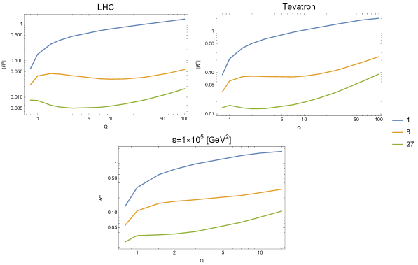
Figure 12: Absolute values of $R^{\alpha}$ given by (60) ($R^{27}$ is negative, the others are strictly positive) at LHC, Tevatron and $s=1\cdot 10^{5}\ \left[GeV^{2}\right]$ kinematics for $Q_{1}^{2}=Q_{2}^{2}=Q^{2}$, $x_{1}=x_{2}=x$ and $N=3$. The values of $R^{8_{a}}$ and $R^{8_{s}}$ are very similar and therefore only $R^{8_{a}}$ is shown on the graph. The plot is logarithmic in both axes.

We see that the singlet distribution is much larger than the octet and $27$ representation. But we also see that the non-singlet distribution values stay the same and even slowly increase at high energy (as predicted). This behavior is unlike what is expected from the non-singlet DPDs that should be highly suppressed at high energies [13, 12]. The source of the seen minimum value of the non-singlet functions is due to the normalization, $G_{p}^{G}\left(x,Q^{2}\right)$ as a function of $Q$ (when is taken $x=\sqrt{\frac{4\cdot Q^{2}}{s}}$).

It’s also interesting to look at the $k$ behavior of the integrand of (LABEL:eq:D_1-2) to explicitly see which splitting scales contribute the most to ${}_{\left[1\right]}^{\alpha}\overline{D}_{h}^{GG}$. The value of this integrand (after performing the $z_{1}$ and $z_{2}$ integrals) is shown on the left of figure 13 for the LHC kinematics and $Q=50\ [GeV]$ (similar behavior is also seen for different kinematics). It can be seen from this figure that the singlet distribution gets most of the contribution from the low $k$ region. In contrast, the non singlet distributions are suppressed at low $k$ and get notable contributions only starting at $k>5\ [GeV]$. The $k$ for which the maximal value of the integrand is obtained is shown in figure 13 on the right for different values of $Q$ at the LHC kinematics. As is expected the dominant splitting scale increases with $Q$.

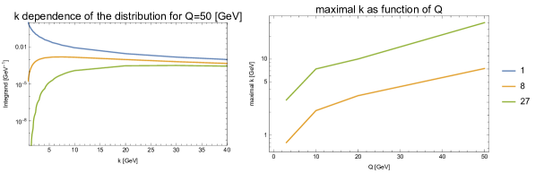
Figure 13: On the left: the integrand of (LABEL:eq:D_1-2), after performing the $z_{1}$ and $z_{2}$ integrals, in the LHC kinematics and $Q=50\ [GeV]$ for different representations and values of $k$. On the right: The value of $k$ for which the maximal value of this integrand is obtained as a function of $Q$.

IV.3 Contribution of Different Color Channels

We want to check the contribution of different color channels both in relation to the interference amplitude contribution and to the cross section given in (70). To this end define (where there is no summation over $\alpha$ unless explicitly indicated):

$$\rho^{\alpha}\coloneqq\frac{\sigma_{I}^{\alpha}}{\sigma_{I}^{1}}=\frac{\sigma_{I}^{\alpha}/\sigma_{1}\sigma_{2}}{\sigma_{I}^{1}/\sigma_{1}\sigma_{2}}=\frac{2\cdot R^{\alpha}\hat{\mathcal{R}}_{I}^{\alpha}}{\left(1+2\cdot R^{1}\right)\hat{\mathcal{R}}_{I}^{1}},$$ (89a)

$$\rho^{all}:=\sum_{\alpha\neq 1}\rho^{\alpha}.$$ (89b)

Here:

• $\sigma_{I}^{\alpha}$ is the contribution of different color channels to the interference diagram and is given by (70). As we explained there is no non-singlet contribution to the non-interference diagram. In particular $\sigma_{I}^{1}$ is the contribution of the singlet channel to the interference diagram.

• $\hat{\mathcal{R}}_{I}^{\alpha}$ is the “hard cross section ratios” defined in (68) and given in table 5.

• $R^{\alpha}$ is the “distributions ratio” defined in (60) and was computed in the previous section.

$\rho^{\alpha}$ represents the relative contributions of non-singlet channels to the interference diagram related to that of the singlet channel. This quantity is however not directly related to the total cross section because we need to consider also the contribution of the non-interference diagram. Therefore we also define:

$$\mathsf{R}_{tot}^{\alpha}\coloneqq\frac{\sigma_{I}^{\alpha}}{\sigma_{R;2+2}}=2\cdot R^{\alpha}\hat{\mathcal{R}}_{I}^{\alpha},$$ (90a)

$$\mathsf{R}_{tot}^{all}\coloneqq\sum_{\alpha\neq 1}\mathsf{R}_{tot}^{\alpha}.$$ (90b)

Here $\sigma_{R;2+2}$ is the contribution of the $2+2$ process to the non-interference diagram (i.e the parton model factorized term), which is given in (65). $\mathsf{R}_{tot}^{\alpha}$ and $\mathsf{R}_{tot}^{all}$ represents the contributions of the non-singlet channels to the cross section in a naive, factorizable parton model. It should be stressed that we expect neither $\mathsf{R}_{tot}^{\alpha}$ or $\rho^{\alpha}$ to be monotonic as a function of $Q$, this is because $R^{\alpha}$ is not monotonic for every $\alpha\neq 1$ (as can be seen from figure 12).

We can now compute $\rho^{\alpha},\rho^{all},\mathsf{R}_{tot}^{\alpha}$ and $\mathsf{R}_{tot}^{\alpha}$ for the different kinematics, the results for $\rho^{\alpha}$ and $\rho^{all}$ are given in figures 14-16 for all the processes considered in table 5 except for the process $\chi_{0}\ +\ J/\psi$ for which $\rho^{\alpha}$ is not well defined (as $\hat{\mathcal{R}}_{I;\chi_{0}+J/\psi}^{1}=0$). The results for $\mathsf{R}_{tot}^{\alpha}$ and $\mathsf{R}_{tot}^{all}$ are given in figures 17-19 for every process except $\chi_{0}\ +\ J/\psi$, and in figure 20 for this process alone.

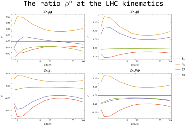
Figure 14: $\rho^{\alpha}=\frac{\sigma_{I}^{\alpha}}{\sigma_{I}^{1}}$, the ratio of non-singlet to singlet contributions in the interference diagram, defined in (89a) as a function of $Q$ (at logarithmic scale) for different processes at the LHC kinematics. The non-monotonic nature of this diagram is the result of the fact that $R^{\alpha}$ is non-monotonic.

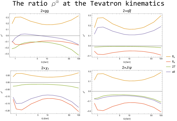
Figure 15: $\rho^{\alpha}=\frac{\sigma_{I}^{\alpha}}{\sigma_{I}^{1}}$, the ratio of non-singlet to singlet contributions in the interference diagram, defined in (89a) as a function of $Q$ (at logarithmic scale) for different processes at the Tevatron kinematics. The non-monotonic nature of this diagram is the result of the fact that $R^{\alpha}$ is non-monotonic.

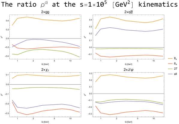
Figure 16: $\rho^{\alpha}=\frac{\sigma_{I}^{\alpha}}{\sigma_{I}^{1}}$, the ratio of non-singlet to singlet contributions in the interference diagram, defined in (89a) as a function of $Q$ (at logarithmic scale) for different processes at the $s=1\cdot 10^{5}\ \left[GeV^{2}\right]$ kinematics. The non-monotonic nature of this diagram is the result of the fact that $R^{\alpha}$ is non-monotonic.

As can be seen from figure 14 the total contribution at the LHC to the interference diagram can be about $5-10\%$ of that of the singlet channel (with individual channels as big as $20\%$), depending on the process. This statement is true even at high $Q^{2}$, the value does not decrease but rather stays approximately constant as a function of $Q^{2}$. The non-singlet contribution increases relatively to the singlet contribution to the interference diagram when considering smaller hadron energies $s$. For example $\rho_{I}^{all}$ of about $10-20\%$ at the Tevatron (figure 15) and even as high as $30\%$ at $s=1\cdot 10^{5}\ [GeV]$.

To see, however, how much this effect is observable in actual processes we need to compare the contributions of the non-singlet channels to that of the total cross section (which includes also the regular non-interference diagram) using $\mathsf{R}_{tot}^{\alpha}$ (90a).

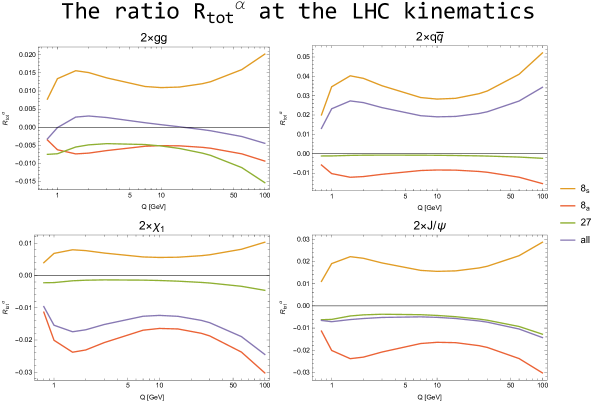
Figure 17: $\mathsf{R}_{tot}^{\alpha}=\frac{\sigma_{I}^{\alpha}}{\sigma_{R;2+2}}$, the ratio of the non-singlet contributions to the $2+2$ process (the parton model factorized cross section, that gets only singlet contributions), defined in (90a) as a function of $Q$ (at logarithmic scale) for different processes at the LHC kinematics. The non-monotonic nature of this diagram is the result of the fact that $R^{\alpha}$ is non-monotonic.

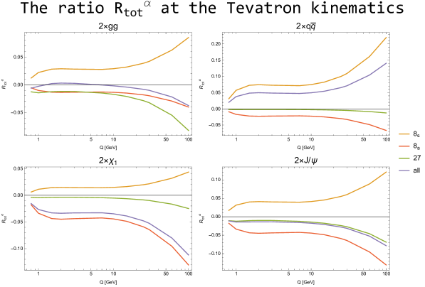
Figure 18: $\mathsf{R}_{tot}^{\alpha}=\frac{\sigma_{I}^{\alpha}}{\sigma_{R;2+2}}$, the ratio of the non-singlet contributions to the $2+2$ process (the parton model factorized cross section, that gets only singlet contributions), defined in (90a) as a function of $Q$ (at logarithmic scale) for different processes at the Tevatron kinematics. The non-monotonic nature of this diagram is the result of the fact that $R^{\alpha}$ is non-monotonic.

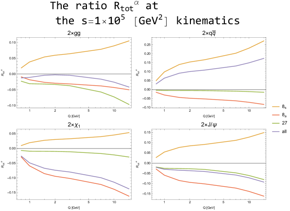
Figure 19: $\mathsf{R}_{tot}^{\alpha}=\frac{\sigma_{I}^{\alpha}}{\sigma_{R;2+2}}$, the ratio of the non-singlet contributions to the $2+2$ process (the parton model factorized cross section, that gets only singlet contributions), defined in (90a) as a function of $Q$ (at logarithmic scale) for different processes at the $s=1\cdot 10^{5}\ \left[GeV^{2}\right]$ kinematics. The non-monotonic nature of this diagram is the result of the fact that $R^{\alpha}$ is non-monotonic.

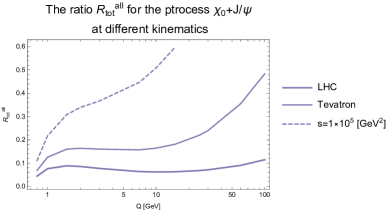
Figure 20: $\mathsf{R}_{tot}^{all}=\underset{\alpha\neq 1}{\sum}\frac{\sigma_{I}^{\alpha}}{\sigma_{R;2+2}}$, the ratio of the non-singlet contributions to the $2+2$ process (the parton model factorized cross section, that gets only singlet contributions), defined in (90a) as a function of $Q$ (at logarithmic scale) for the $\chi_{0}\ +\ J/\psi$ process at different kinematics (LHC, Tevatron and $s=1\cdot 10^{5}\ \left[GeV^{2}\right]$). The non-monotonic nature of this diagram is the result of the fact that $R^{\alpha}$ is non-monotonic.

The total contribution to the cross section of non-singlet channels is about $2\%$ for most processes at the LHC (figure 17). At lower $s$ this contribution somewhat increases, as was the case for $\rho^{\alpha}$. At Tevatron kinematics, $\mathsf{R}_{tot}^{\alpha}$ is $5-10\%$ for most cases as can be seen in figure 18. At even lower $s=1\cdot 10^{5}\ [GeV]$ (figure 18) this trend continues but more slowly as can be seen from the similar values between figure 19 and 18.

On contrary, we find that non-singlet color contributions are strongest when one considers the production of a $\chi_{0}$ together with a quarkonia state whose quantum numbers require the production of additional soft gluon (e.g $J/\psi$ and $\chi_{1}$). For the $\chi_{0}\ +\ J/\psi$ process the contribution is significantly larger than for other processes (the reason for which was discussed in section IV.1) as can be seen in figure 20: about $10\%$ at LHC, up to $50\%$ at the Tevatron and even $60\%$ when $s=1\cdot 10^{5}\ [GeV]$.

It’s interesting to note that although $\mathsf{R}_{tot}^{\alpha}$ is smaller compared to the singlet contributions for all the processes it’s somewhat increasing in $Q^{2}$ for a constant value of $s$. This statement is, again as explained above, contrasted to the regular color non-singlet $2\rightarrow 2$ distributions which should strongly decrease with the increasing $Q$ [13, 11].

V Conclusion

In this paper, we studied the contribution of color correlations in the 4 jet and double quarkonium states in DPS. We have considered the case of symmetric kinematics, when $x_{1}=x_{2}=x_{3}=x_{4}=x$ and $Q_{1}=Q_{2}=Q$ where we expect that the effect of the color correlations will be the biggest one. We see that the contribution of the color correlations is due to the interference diagrams where the two hard processes essentially overlap contrary to conventional DPS where the two hard processes completely factorize. Consequently, the DPS LLA cross section due to color singlet correlations depends only on transverse scales and very weakly depends on $\frac{x_{1}}{x_{2}}$ and $\frac{x_{3}}{x_{4}}$. For interference contributions, we expect their contributions rapidly decrease away from the central kinematics point which may be one of the ways to detect them.

We have seen that it is possible to avoid the conventional Sudakov suppression of color correlations, by considering specific $1\rightarrow 2$ processes depicted in figure 2, however also such processes do not decrease with the increase of the transverse scale, they are still small due to the relative smallness of interference diagrams in the hard process. We saw that in the Tevatron and LHC kinematics they amount to renormalization of 2-5% of the mean field DPS cross section. We have also seen that the contribution of different channels to cross sections may be larger, up to 10-15%, but different contributions partly cancel each other since the contribution of the color correlation to GPD and total cross section can be both positive and negative, depending on the representation of the color channel. The color correlation contribution increases if we go to smaller energies, however, we must remember that for smaller energies there might be not enough statistics to observe DPS.

Nevertheless, the fact that perturbative color correlations do not decrease with transverse scale makes it potentially possible to observe them and thus have further insight into the precise QCD description of the nucleon wave functions.

We also consider the contribution of the color correlations to double charmonium production. Indeed there is a well known problem in the theory of DPS–to describe the very large DPS cross section of double charmonium production observed in central LHC kinematics [42]. However, we see that color correlations contribute only at most several percent to double charmonium production even at smaller transverse scales and do not solve the problem.

In order to calculate the corresponding color correlations we develop formalism based on the “DDT” formula, which in the leading logarithmic approximation (LLA) for total inclusive cross section is equivalent to the TMD approach. In fact, the “DDT” formula (after resummations) is the solution of the Collins-Soper equations for TMD in LLA [43]. It will be interesting to further study the perturbative color correlations away from the central kinematics considered in this paper, as well as to study further the color correlations in $1\rightarrow 2$ processes in double $\chi_{0}$ process [11].

Finally, it will be interesting to consider the contribution of color correlations for the case of nondiagonal GPD along the lines of [44].

Appendix A Color Kernels

We now turn to compute explicitly the factors $\phantom{}{}^{\alpha}\overline{C}_{A}^{B}$ for different representations. These factors were derived partially in [11] for polarized particles and completely in [15]. In this section we rederive them in our formalism for completeness. Let it be remind that for the singlet representation (as in the original DGLAP case), these factors are shown in table 6.

R	1
$C_{F}^{F}$	$\frac{N^{2}-1}{2N}$
$C_{F}^{G}$	$\frac{N^{2}-1}{2N}$
$C_{G}^{F}$	$\frac{1}{2}$
$C_{G}^{G}$	$N$

Table 6: Color factors for the singlet representation

We start by considering the simplest case of $R=27$, $q\overline{q}$ cannot be in this representation, and therefore $\phantom{}{}^{27}\overline{C}_{F}^{F}=\phantom{}^{27}\overline{C}_{G}^{F}=\phantom{}^{27}\overline{C}_{F}^{G}=0$. In order to find the only non-zero kernel $\phantom{}{}^{27}\overline{C}_{G}^{G}$ attach the $27$ projector to a gluon ladder, as shown in fig. 21. The color factor for such a diagram is well known [33, 32] and equal to $\phantom{}{}^{27}\overline{C}_{G}^{G}=-1$ . This result is a special case of the “interaction force identity”, as will be explained in Appendix F.

Figure 21: The ladder diagram that determines $\overline{C}_{G}^{G}\left(27\right)$, $P^{27}$ is the 2 gluon projector to the irreducible representation $27$.

By the same line of argument $\phantom{}{}^{10}\overline{C}_{F}^{F}=\phantom{}^{10}\overline{C}_{G}^{F}=\phantom{}^{10}\overline{C}_{F}^{G}=\phantom{}^{10}\overline{C}_{G}^{G}=0$ where $10$ is the sum of the irreducible decouple representations [32], we, therefore, conclude that the representation $10$ does not evolve in ladders and should not contribute to physical processes. We now turn to consider the octet representation of quarks and the symmetric octet ($8_{s}$) and anti-symmetric octet ($8_{a}$) of gluons. Considering these representations raises two problems that were absent when we considered the $27$ and $10$ representations:

• There is now a mixing of quark and gluons, this poses a certain ambiguity to the $\overline{C}_{G}^{F},\ \overline{C}_{F}^{G}$ kernels.

• The second problem is that the single quark octet representation mixes with the two gluon octet representations. This effect potentially could make $\overline{C}_{F}^{G}$ a matrix connecting two representations rather than a simple factor, which would ruin the analysis made in section II.1.

We’ll delay the solution of the first problem to the end of this section, and until then keep the freedom of normalization of these kernels. As for the second problem, luckily it can be solved easily. This solution is done by considering, instead of quark or anti-quark ladders separately, the sum of quark and anti quark ladders, as shown in fig. 22. This solution, although very elegant, works only as long as there is symmetry between quarks and anti-quarks. When such symmetry breaks (for example when considering the valence parton distribution) it will no longer work. In this paper, we consider kinematic regions where valence distribution is small compared to gluon or sea distributions.

Figure 22: The DGLAP ladders associated with $\overline{C}_{G}^{G}\ (a)$, $\overline{C}_{G}^{F}\ (b)$, $\overline{C}_{F}^{G}\ (c)$ and $\overline{C}_{F}^{F}\ (d)$, where we have summed quark and anti-quark ladders together.

A.1 Color Factor for the $8_{a}$ Representation

We start by concretely looking at the $8_{a}$ representation. Consider the two structures $G_{a}$ and $Q_{a}$ that represent this representation for quarks and gluons, as shown in fig 23. We’ll show that these structures propagate within the ladder and do not mix with any other structures. The color kernels for $8_{a}$ will be the contractions of these structures with the ladders given in figure 22.

Figure 23: The anti-symmetric octet ($8_{a}$) structures $G_{a}\ (a)$ and $Q_{a}\ (b)$. $\alpha$ and $\beta$ are arbitrary real numbers.

A.1.1 $\overline{C}_{G}^{G}$

Figure 24: Contraction of $\Phi_{G}^{G}$ with $G_{a}$

We now contract the ladder of type $\Phi_{G}^{G}$ with the color structure $G$ as seen in figure 24:

$$G_{a}^{bc}\cdot V_{bc;gf}=i\alpha f^{bca}\left(c_{\alpha}P_{bc;gf}^{\alpha}\right).$$ (91)

We use the contraction property of the projectors (the generalized version as proved in section F) to cancel every projector but $8_{a}$ and are left with:

$$=i\alpha f^{bca}c_{8_{a}}P_{bc;gf}^{8_{a}}=i\alpha c_{8_{a}}\left(f^{bca}\frac{f^{bce}f^{gfe}}{N}\right)=c_{8_{a}}\left(\alpha iN\frac{f^{gfa}}{N}\right)=c_{8_{a}}G_{gf}.$$

Here, as we’ll see in Appendix F, $c_{8_{a}}=\frac{N}{2}$.

A.1.2 $\overline{C}_{F}^{G}$

Figure 25: Contraction of $\Phi_{F}^{G}$ with $G_{a}$

This contraction is shown in figure 25 and is written as:

$$i\alpha f^{bca}\left(t_{ik}^{c}t_{kj}^{b}+t_{jk}^{b}t_{ki}^{c}\right)=-\alpha if^{cba}t_{ik}^{c}t_{kj}^{b}+if^{bca}t_{jk}^{b}t_{ki}^{c}=\alpha\frac{N}{2}\left(t_{ij}^{e}-t_{ji}^{e}\right)=\frac{\alpha}{\beta}\frac{N}{2}Q_{ij}.$$ (92)

So we get that $\overline{C}_{F}^{G}=\frac{\alpha}{\beta}\frac{N}{2}$.

A.1.3 $\overline{C}_{F}^{F}$

This contraction is viewed on figure 26 and is written as:

Figure 26: Contraction of $\Phi_{F}^{F}$ with $Q_{a}$

$$Q_{a}^{ij}\left(t_{ik}^{e}t_{lj}^{e}+t_{ki}^{e}t_{jl}^{e}\right) =\beta\left(t_{kl}^{a}t_{ik}^{e}t_{lj}^{e}-t_{lk}^{a}t_{ki}^{e}t_{jl}^{e}\right)=\beta\left(t_{ik}^{e}t_{kl}^{a}t_{lj}^{e}-t_{jl}^{e}t_{lk}^{a}t_{ki}^{e}\right)$$

$$=-\beta\frac{1}{2N}\left(t_{ij}^{a}-t_{ji}^{a}\right)=-\frac{1}{2N}Q_{ij}.$$ (93)

So the factor is $\overline{C}_{F}^{F}=-\frac{1}{2N}$.

A.1.4 $\overline{C}_{G}^{F}$

This contraction is viewed on figure 27 and is written as

Figure 27: Contraction of $\Phi_{G}^{F}$ with $Q_{a}$

$$Q_{a}^{ij}\left(t_{jk}^{b}t_{ki}^{c}+t_{ik}^{c}t_{kj}^{b}\right) =\beta\left(t_{ij}^{a}t_{jk}^{b}t_{ki}^{c}-t_{ji}^{a}t_{ik}^{c}t_{kj}^{b}\right)$$

$$=\beta\left(tr\left[t^{a}t^{b}t^{c}\right]-tr\left[t^{a}t^{c}t^{b}\right]\right)$$

$$=\beta\frac{1}{4}\left(if^{abc}+d^{abc}-if^{acb}-d^{acb}\right)$$

$$=\beta\frac{i}{4}\left(f^{abc}-f^{acb}\right)$$

$$=\beta\frac{i}{2}f^{bca}$$

$$=\frac{\beta}{\alpha}\frac{1}{2}G_{bc}.$$ (94)

So the factor is $\overline{C}_{G}^{F}=\frac{\beta}{\alpha}\frac{1}{2}$.

A.2 Color Factor for the $8_{s}$ Representation

We now look at the $8_{s}$ representation. Consider two new structures $G_{s}$ and $Q_{s}$ that represent this representation for gluon and quark, as shown in fig 28. The rest of the analysis is the same.

Figure 28: The symmetric octet ($8_{s}$) structures $G_{s}\ (a)$ and $Q_{s}\ (b)$. $\alpha$ and $\beta$ are arbitrary real numbers that are not necessarily the same as for $8_{a}$.

A.2.1 $\overline{C}_{G}^{G}$

Figure 29: Contraction of $\Phi_{G}^{G}$ with $G_{s}$

We now contract the ladder of type $\Phi_{G}^{G}$ with the color structure $G_{s}$ as seen in figure 29:

$$G_{s}^{bc}\cdot V_{bc;gf}=\alpha d^{bca}\left(c_{\alpha}P_{bc;gf}^{\alpha}\right).$$ (95)

We use the contraction property of the projectors (the generalized version) to cancel every projector but $8_{s}$ and are left with:

$$=\alpha d^{bca}c_{8_{s}}P_{bc;gf}^{8_{s}}=\alpha c_{8_{s}}\left(d^{bca}d^{bce}d^{gfe}\frac{N}{N^{2}-4}\right)=c_{8_{s}}\left(\alpha\frac{N^{2}-4}{N}d^{gfa}\frac{N}{N^{2}-4}\right)=c_{8_{s}}G_{gf}^{s}.$$

Where, as we have seen $c_{8_{s}}=\frac{N}{2}$.

A.2.2 $\overline{C}_{F}^{G}$

Figure 30: Contraction of $\Phi_{F}^{G}$ with $G_{s}$

This contraction is shown in figure 30 and is written as:

$$\alpha d^{bca}\left(t_{ik}^{c}t_{kj}^{b}+t_{jk}^{b}t_{ki}^{c}\right)=\alpha\left(d^{cba}t_{ik}^{c}t_{kj}^{b}+d^{bca}t_{jk}^{b}t_{ki}^{c}\right)=\alpha\frac{N^{2}-4}{2N}\left(t_{ij}^{e}+t_{ji}^{e}\right)=\frac{\alpha}{\beta}\frac{N^{2}-4}{2N}Q_{ij}^{s}.$$ (96)

So we get that $\overline{C}_{F}^{G}=\frac{N^{2}-4}{2N}$.

A.2.3 $\overline{C}_{F}^{F}$

This contraction is viewed on figure 31 and is written as:

Figure 31: Contraction of $\Phi_{F}^{F}$ with $Q_{s}$

$$Q_{s}^{ij}\left(t_{ik}^{e}t_{lj}^{e}+t_{ki}^{e}t_{jl}^{e}\right) =\beta\left(t_{kl}^{a}t_{ik}^{e}t_{lj}^{e}+t_{lk}^{a}t_{ki}^{e}t_{jl}^{e}\right)$$

$$=\beta\left(t_{ik}^{e}t_{kl}^{a}t_{lj}^{e}+t_{jl}^{e}t_{lk}^{a}t_{ki}^{e}\right)$$

$$=-\frac{\beta}{2N}\left(t_{ij}^{a}+t_{ji}^{a}\right)=-\frac{1}{2N}Q_{ij}^{s}.$$ (97)

So the factor is $\overline{C}_{F}^{F}=-\frac{1}{2N}$.

A.2.4 $\overline{C}_{G}^{F}$

This contraction is viewed on figure 32 and is written as

Figure 32: Contraction of $\Phi_{G}^{F}$ with $Q_{s}$

$$Q_{s}^{ij}\left(t_{jk}^{b}t_{ki}^{c}+t_{ik}^{c}t_{kj}^{b}\right) =\beta\left(t_{ij}^{a}t_{jk}^{b}t_{ki}^{c}+t_{ji}^{a}t_{ik}^{c}t_{kj}^{b}\right)=$$

$$=\beta\left(tr\left[t^{a}t^{b}t^{c}\right]+tr\left[t^{a}t^{c}t^{b}\right]\right)$$

$$=\beta\frac{1}{4}\left(if^{abc}+d^{abc}+if^{acb}+d^{acb}\right)$$

$$=\beta\frac{i}{4}\left(d^{abc}+d^{acb}\right)$$

$$=\beta\frac{1}{2}d^{abc}$$

$$=\frac{\beta}{\alpha}\frac{1}{2}G_{bc}^{s}$$ (98)

So the factor is $\overline{C}_{G}^{F}=\frac{\beta}{\alpha}\frac{1}{2}G_{bc}^{s}$.

A.3 Normalization of $\overline{C}_{F}^{G}$ and $\overline{C}_{G}^{F}$

Note that the color factors given above for $\overline{C}_{F}^{G}$ and $\overline{C}_{G}^{F}$ are not well defined and depend on the ratio of $\frac{\alpha}{\beta}$ which was arbitrary. Therefore only the multiplication $C_{G}^{F}\cdot C_{F}^{G}$ is well defined. In order to derive well defined color factors we impose the condition that a ladder would be well defined independently of whether we go from quark to gluon or from gluon to quark as shown in figure 33.

Figure 33: gluon to quark ladder diagram.

In our convention the ladder end in the hard process and therefore we sum over the color (and flavor) indices of the final (superscript) parton type and average over the color (and flavor) indices of the initial (subscript) parton type. This convention means that if we take the diagram in figure 33 from above or from below it will be equal only if we compensate for the averaging of the initial parton (and therefore effectively summing for both initial and final parton color and flavor indices):

$$\underset{"types"\ of\ quarks}{\underbrace{N}}\overline{\Phi}_{F}^{G}=\underset{"types"\ of\ gluons}{\underbrace{\left(N^{2}-1\right)}}\overline{\Phi}_{G}^{F}.$$ (99)

The $z$ part of this argument is true[19] so we’ll ignore it and get for the color-flavor part:

$$N\overline{C}_{F}^{G}=\left(N^{2}-1\right)\overline{C}_{G}^{F},$$ (100)

$$\frac{\overline{C}_{F}^{G}}{\overline{C}_{G}^{F}}=\frac{N^{2}-1}{N}.$$ (101)

Note that this equation is actually independent of the color channel and therefore should be true for both the singlet and octet channels. Indeed for the singlet channel we have:

$$\frac{\overline{C}_{F}^{G}}{\overline{C}_{G}^{F}}=\frac{\frac{N^{2}-1}{2N}}{\frac{1}{2}}=\frac{N^{2}-1}{N}.$$ (102)

A.3.1 $8_{a}$

Now the color factor multiplication is $\overline{C}_{F}^{G}\overline{C}_{G}^{F}=\frac{N}{4}$, therefore we can solve:

$$\phantom{}{}^{8_{a}}\overline{C}_{G}^{F}=\frac{1}{2}\sqrt{\frac{N^{2}}{2\left(N^{2}-1\right)}},$$ (103a)

$$\phantom{}{}^{8_{a}}\overline{C}_{F}^{G}=\sqrt{\frac{N^{2}-1}{8}}.$$ (103b)

A.3.2 $8_{s}$

Now the color factor multiplication is $\overline{C}_{F}^{G}\overline{C}_{G}^{F}=\frac{N^{2}-4}{4N}$, therefore we can solve:

$$\phantom{}{}^{8_{s}}\overline{C}_{G}^{F}=\frac{1}{2}\sqrt{\frac{N^{2}-4}{2\left(N^{2}-1\right)}},$$ (104a)

$$\phantom{}{}^{8_{s}}\overline{C}_{F}^{G}=\frac{1}{2N}\sqrt{\frac{\left(N^{2}-4\right)\left(N^{2}-1\right)}{2}}.$$ (104b)

Appendix B Formal Derivation of the Non-Singlet DGLAP Equation

In this section, we give a more detailed and formal derivation of (5). We start with the Bethe-Salpeter equation for $D_{A}^{B}$, the singlet structure function, that comes from considering ladder type diagrams [19]:

$$D_{A}^{B}\left(x,k_{0}^{2}\right)=\delta_{A}^{B}\left(1-x\right)d_{A}\left(k_{0}^{2}\right)+d_{A}\left(k_{0}^{2}\right)\sum_{C}\intop_{zk_{0}^{2}}^{Q^{2}}\frac{dk^{2}}{k^{2}}\intop_{0}^{1}\frac{dz}{z}A_{A}^{C}d_{A}^{-1}\left(\frac{k^{2}}{z}\right)\Phi_{A}^{C}\left(z\right)D_{C}^{B}\left(\frac{x}{z},k^{2}\right).$$ (105)

Here:

• $d_{A}$ is the renormalization of particle $A$.

• $A_{A}^{C}=d_{A}\left(\frac{k^{2}}{z}\right)d_{C}\left(k^{2}\right)d_{G}\Gamma^{2}$ is the renormalization of the ladder, which we take to be $\frac{\alpha\left(k^{2}\right)}{4\pi}$.

• $\Phi_{A}^{C}\left(z\right)=C_{A}^{B}\cdot V\left(z\right)$ is the singlet splitting function as explained in the text.

• $A,B,C$ are types of partons, e.g gluon, quark, anti-quark.

$d_{A}$ obeys the relation [19]:

$$\frac{\partial}{\partial ln\left(k_{0}^{2}\right)}d_{A}^{-1}\left(k_{0}^{2}\right)=-d_{A}^{-1}\left(k_{0}^{2}\right)\sum_{C}\intop_{0}^{1}z\frac{\alpha\left(k_{0}^{2}\right)}{4\pi}\Phi_{A}^{C}\left(z\right)dz.$$ (106)

This equation represents virtual corrections of the parton to itself and therefore is true even if the parton is in a non-singlet state with its complex conjugate (see figure 4.$(b)$ ). therefore for a general channel the only part of equation (105) that changes is the one dependent on the real (ladder, see figure 4.$(a)$ ) contributions:

$$\overline{D}_{A}^{B}\left(x,k_{0}^{2}\right)=\delta_{A}^{B}\left(1-x\right)d_{A}\left(k_{0}^{2}\right)+d_{A}\left(k_{0}^{2}\right)\sum_{C}\intop_{zk_{0}^{2}}^{Q^{2}}\frac{dk^{2}}{k^{2}}\intop_{0}^{1}\frac{dz}{z}\frac{\alpha\left(k^{2}\right)}{4\pi}d_{A}^{-1}\left(\frac{k^{2}}{z}\right)\overline{\Phi}_{A}^{C}\left(z\right)\overline{D}_{C}^{B}\left(\frac{x}{z},k^{2}\right).$$ (107)

Note that $d_{A}$ still obeys (106) with the singlet ($\Phi_{A}^{C}$) splitting function. Trivially:

$$d_{A}\left(k_{0}^{2}\right)\frac{\partial}{\partial ln\left(k_{0}^{2}\right)}\left[\overline{D}_{A}^{B}\left(x,k_{0}^{2}\right)d_{A}^{-1}\left(k_{0}^{2}\right)\right]=\overline{D}_{A}^{B}\left(x,k_{0}^{2}\right)d_{A}\left(k_{0}^{2}\right)\frac{\partial d_{A}^{-1}\left(k_{0}^{2}\right)}{\partial ln\left(k_{0}^{2}\right)}+\frac{\partial\overline{D}_{A}^{B}\left(x,k_{0}^{2}\right)}{\partial ln\left(k_{0}^{2}\right)}.$$ (108)

Using equation (106) and (107) we can write:

$$-\sum_{C}\intop_{0}^{1}\frac{dz}{z}\frac{\alpha\left(k_{0}^{2}\right)}{4\pi}\overline{\Phi}_{A}^{C}\left(z\right)\overline{D}_{C}^{B}\left(\frac{x}{z},k_{0}^{2}\right)=-\overline{D}_{A}^{B}\left(x,k_{0}^{2}\right)\sum_{C}\intop_{0}^{1}z\frac{\alpha\left(k_{0}^{2}\right)}{4\pi}\Phi_{A}^{C}\left(z\right)dz+\frac{\partial\overline{D}_{A}^{B}\left(x,k_{0}^{2}\right)}{\partial ln\left(k_{0}^{2}\right)},$$ (109)

$$\frac{\partial\overline{D}_{A}^{B}\left(x,k_{0}^{2}\right)}{\partial ln\left(k_{0}^{2}\right)}=-\frac{\alpha\left(k_{0}^{2}\right)}{4\pi}\sum_{C}\intop_{0}^{1}\frac{dz}{z}\left[\overline{\Phi}_{A}^{C}\left(z\right)\overline{D}_{C}^{B}\left(\frac{x}{z},k_{0}^{2}\right)-z^{2}\Phi_{A}^{C}\left(z\right)\overline{D}_{A}^{B}\left(x,k_{0}^{2}\right)\right].$$ (110)

Using (6) eq. (110) can be written as:

$$\frac{\partial D_{A}^{B}\left(x,k_{0}^{2}\right)}{\partial ln\left(k_{0}^{2}\right)}=K_{1}+K_{2},$$ (111a)

$$K_{1}=-\frac{\alpha\left(k_{0}^{2}\right)}{4\pi}\sum_{C}\intop_{0}^{1}\frac{dz}{z}\overline{\Phi}_{A}^{C}\left(z\right)\left[\overline{D}_{C}^{B}\left(\frac{x}{z},k_{0}^{2}\right)-z^{2}\overline{D}_{A}^{B}\left(x,k_{0}^{2}\right)\right],$$ (111b)

$$K_{2}=-\overline{D}_{A}^{B}\left(x,k_{0}^{2}\right)\frac{\alpha\left(k_{0}^{2}\right)}{4\pi}\sum_{C}\intop_{0}^{1}dzV_{A}^{C}\left(z\right)z\left[C_{A}^{C}-\overline{C}_{A}^{C}\right].$$ (111c)

The first part is finite as $z\rightarrow 1$ and is just the regular DGLAP equation with the new kernels (which are given in table 2). The second part diverges as $z\rightarrow 1$ and therefore we need to regularize it. We’ll keep the regularization given in[19]:

• Integration of $z$ up to $1-\frac{\lambda^{2}}{k_{0}^{2}}$, for $\lambda$ an IR cutoff regulator

• Adding a non zero $\Delta$ in $V_{A}^{B}\left(z\right)\rightarrow V_{A}^{B}\left(z,\Delta\right)$ for $\Delta=\frac{zk_{0}^{2}}{\sigma_{k_{0}}}$ (where $\sigma_{k_{0}}=\frac{\left(2k_{0}c\right)^{2}}{c^{2}}\approx Q^{2}$, for $c$ the gauge fixing vector)

Define the Sudakov suppression factor:

$$\overline{S}_{A}\left(k_{0}^{2},Q^{2}\right)=e^{-\sum_{C}\left(C_{A}^{C}-\overline{C}_{A}^{C}\right)\intop_{k_{0}^{2}}^{Q^{2}}\frac{dk^{2}}{k^{2}}\frac{\alpha\left(k^{2}\right)}{4\pi}\intop_{x}^{1-\frac{\lambda^{2}}{k_{0}^{2}}}dzzV_{A}^{C}\left(z,\frac{zk_{0}^{2}}{\sigma_{k_{0}}}\right)}$$ (112)

Which is a properly regularized version of the version appearing in the text. Then for $\overline{D}_{A}^{B}\left(x,k_{0}^{2}\right)=\overline{S}_{A}\left(k_{0}^{2},Q^{2}\right)\widetilde{D}_{A}^{B}\left(x,k_{0}^{2}\right)$ eq. (110) is reduced to (10).

Appendix C $\widetilde{D}_{A}^{B}$ at the Limit $x\rightarrow 1$

In this section, we write a derivation of (14) as the derivation in [19] is only partial, hard to generalize for different color factors, and does not include $\widetilde{D}_{G}^{G}$. For reference we write the standard solutions of (10) in Mellin space:

$$\widetilde{D}_{F}^{F}\left(j,\xi\right) =\widetilde{D}^{sea}\left(j,\xi\right)+\widetilde{D}^{val}\left(j,\xi\right)$$ (113a)

$$\widetilde{D}^{val}\left(j,\xi\right) =e^{\overline{\nu}_{0}\xi}$$ (113b)

$$\widetilde{D}^{sea}\left(j,\xi\right) =\frac{1}{2n_{f}}\left[\frac{\overline{\nu}_{0}-\overline{\nu}_{-}}{\overline{\nu}_{+}-\overline{\nu}_{-}}e^{\overline{\nu}_{+}\xi}+\frac{\overline{\nu}_{+}-\overline{\nu}_{0}}{\overline{\nu}_{+}-\overline{\nu}_{-}}e^{\overline{\nu}_{-}\xi}-e^{\overline{\nu}_{0}\xi}\right]$$ (113c)

$$\widetilde{D}_{G}^{G}\left(j,\xi\right) =\frac{\overline{\nu}_{0}-\overline{\nu}_{-}}{\overline{\nu}_{+}-\overline{\nu}_{-}}e^{\overline{\nu}_{-}\xi}+\frac{\overline{\nu}_{+}-\overline{\nu}_{0}}{\overline{\nu}_{+}-\overline{\nu}_{-}}e^{\overline{\nu}_{+}\xi}$$ (113d)

$$\widetilde{D}_{F}^{G}\left(j,\xi\right) =\frac{\overline{\Phi}_{F}^{G}\left(j\right)}{\overline{\nu}_{+}-\overline{\nu}_{-}}\left[e^{\overline{\nu}_{+}\xi}-e^{\overline{\nu}_{-}\xi}\right]$$ (113e)

$$\widetilde{D}_{G}^{F}\left(j,\xi\right) =\frac{\overline{\Phi}_{G}^{F}\left(j\right)}{\overline{\nu}_{+}-\overline{\nu}_{-}}\left[e^{\overline{\nu}_{+}\xi}-e^{\overline{\nu}_{-}\xi}\right]$$ (113f)

Where $\xi=\frac{3}{\beta_{0}}ln\left[\frac{\alpha\left(k_{0}^{2}\right)}{\alpha\left(Q^{2}\right)}\right]$ and:

$$\overline{\nu}_{0} =\overline{\nu}_{F}=\frac{1}{3}\left(-\left(\frac{6}{j}+\frac{6}{j+1}+12(\psi(j)+\gamma_{E})-17\right)\overline{C}_{F}^{F}-8\overline{C}_{F}^{G}\right)$$ (114a)

$$\overline{\nu}_{G} =-\overline{C}_{G}^{G}\left(-\frac{8\left(j^{2}+j+1\right)}{j\left(j^{2}-1\right)(j+2)}+4\psi(j+1)-\frac{11}{3}+4\gamma_{E}\right)-\frac{4}{3}n_{f}\overline{C}_{G}^{F}$$ (114b)

$$\overline{\Phi}_{F}^{G}\left(j\right) =2\overline{C}_{F}^{G}\frac{j^{2}+j+1}{j\left(j^{2}-1\right)}$$ (114c)

$$\overline{\Phi}_{G}^{F}\left(j\right) =\overline{C}_{G}^{F}\frac{j^{2}+j+2}{j\left(j+1\right)\left(j+2\right)}$$ (114d)

$$\overline{\nu}_{\pm} =\frac{1}{2}\left\{\overline{\nu}_{F}+\overline{\nu}_{G}\pm\sqrt{\left(\overline{\nu}_{F}-\overline{\nu}_{G}\right)^{2}+8n_{f}\overline{\Phi}_{F}^{G}\left(j\right)\overline{\Phi}_{G}^{F}\left(j\right)}\right\}$$ (114e)

Transforming back from Mellin to $x-space$ is by numerically evaluating the inverse Mellin transform:

$$\widetilde{D}_{A}^{B}\left(x,\xi\right)=\intop\frac{dj}{2\pi i}x^{-j}\widetilde{D}_{A}^{B}\left(j,\xi\right).$$ (115)

For the region $x\sim 1$ this integral can be analytically evaluated. We’ll start with $\widetilde{D}^{val}$ , let’s write (115) explicitly in this case:

$$\widetilde{D}^{val}\left(x,\xi\right) =\intop\frac{dj}{2\pi i}x^{-j}e^{\overline{\nu}_{0}\xi}$$

$$=\intop\frac{dj}{2\pi i}e^{\frac{1}{3}\left(-\left(\frac{6}{j}+\frac{6}{j+1}+12(\psi(j)+\gamma_{E})-17\right)\overline{C}_{F}^{F}-8\overline{C}_{F}^{G}\right)\xi-jln\left(x\right)}.$$ (116)

This integral gets the highest contribution form its saddle point, we want to prove that this saddle point is at $j\gg 1$. In order to do that we’ll find the maximum of the argument (aside from the singularity at $j=0$). We’ll assume that this maximum is achieved at very large $j$ and then we will see that there is indeed a maximum at this region, which will justify the assumption. At this region $\frac{6}{j}+\frac{6}{j+1}$ are negligible and we can write $\psi\left(j\right)\approx ln\left(j\right)-\frac{1}{2j}\approx ln\left(j\right)$, therefore:

$$0 =\frac{d}{dj}\left[\frac{1}{3}\left(-\left(12(ln(j)+\gamma_{E})-17\right)\overline{C}_{F}^{F}-8\overline{C}_{F}^{G}\right)\xi-jln\left(x\right)\right]_{j=j_{0}}$$

$$=-4\xi\overline{C}_{F}^{F}\frac{1}{j_{0}}-ln\left(x\right).$$ (117)

So the maximum is at:

$$j_{0}=-\overline{C}_{F}^{F}\frac{4\xi}{ln\left(x\right)}\approx\overline{C}_{F}^{F}\frac{4\xi}{1-x}.$$ (118)

Since $x\sim 1$, $j_{0}$ is very large, and so our assumption that the maximum is at very large $j$ is justified, but only for $\overline{C}_{F}^{F}>0$ (we’ll return to this point later on). If we now assume the major contribution to this integral comes from the proximity of this saddle point we can write it as:

$$\widetilde{D}^{val}\left(x,\xi\right)\approx e^{-\xi\left[-\left(\frac{17}{3}-4\gamma_{E}\right)\overline{C}_{F}^{F}+\frac{8}{3}\overline{C}_{F}^{G}\right]}\frac{1}{2\pi i}\int e^{-4\xi\overline{C}_{F}^{F}ln\left(j\right)-jln\left(x\right)}dj.$$ (119)

Changing $t=jln\left(x\right)$ we get:

$$\widetilde{D}^{val}\left(x,\xi\right)\approx-\frac{1}{2\pi i}\frac{e^{-\xi\left[-\left(\frac{17}{3}-4\gamma_{E}\right)\overline{C}_{F}^{F}+\frac{8}{3}\overline{C}_{F}^{G}\right]}}{ln\left(\frac{1}{x}\right)^{-4\xi\frac{N^{2}-1}{2N}+1}}\int\left(-t\right)^{-4\xi\overline{C}_{F}^{F}}e^{-t}dt.$$ (120)

Using the integral representation of the gamma function $\frac{-2\pi i}{\Gamma\left(z\right)}=\int\left(-t\right)^{-z}e^{-t}dt$ and $ln\left(x\right)\approx x-1$ we write:

$$\widetilde{D}^{val}\left(x,\xi\right)\overset{x\sim 1}{\approx}\frac{e^{-\xi\left[\left(4\gamma_{E}-\frac{17}{3}\right)\overline{C}_{F}^{F}+\frac{8}{3}\overline{C}_{F}^{G}\right]}}{\left(1-x\right)^{1-4\xi\overline{C}_{F}^{F}}\Gamma\left(4\xi\overline{C}_{F}^{F}\right)}.$$ (121)

We can now try to evaluate the other structure functions, in order to do that we’ll evaluate first their components at the region of $j_{0}$. $j_{0}$ is very large so we’ll only keep leading terms in the expressions for $\Phi_{F}^{G}$ and $\Phi_{G}^{F}$:

$$\Phi_{F}^{G}\left(j_{0}\right)=2\overline{C}_{F}^{G}\frac{1}{j_{0}},$$ (122a)

$$\Phi_{G}^{F}\left(j_{0}\right)=2\overline{C}_{G}^{F}\frac{1}{j_{0}}.$$ (122b)

Both are very small and therefore we can approximate using $\sqrt{1+\epsilon}\approx 1+\frac{1}{2}\epsilon$ :

$$\sqrt{\left[\overline{\nu}_{F}-\overline{\nu}_{G}\right]^{2}+8n_{f}\Phi_{F}^{G}\Phi_{G}^{F}}=\left(\overline{\nu}_{F}-\overline{\nu}_{G}\right)\sqrt{1+8n_{f}\frac{\left(\frac{2\overline{C}_{F}^{G}}{j_{0}}\right)\left(\frac{2\overline{C}_{G}^{F}}{j_{0}}\right)}{\left(\overline{\nu}_{F}-\overline{\nu}_{G}\right)^{2}}}\\ \approx\left(\overline{\nu}_{F}-\overline{\nu}_{G}\right)\left[1+\frac{1}{2}8n_{f}\frac{\left(\frac{2\overline{C}_{F}^{G}}{j_{0}}\right)\left(\frac{2\overline{C}_{G}^{F}}{j_{0}}\right)}{\left(\overline{\nu}_{F}-\overline{\nu}_{G}\right)^{2}}\right]=\left(\overline{\nu}_{F}-\overline{\nu}_{G}\right)+16n_{f}\frac{\overline{C}_{F}^{G}\overline{C}_{G}^{F}}{\left(\overline{\nu}_{F}-\overline{\nu}_{G}\right)j_{0}^{2}}.$$ (123)

Which gives:

$$\overline{\nu}_{+}\approx\overline{\nu}_{F}+8n_{f}\overline{C}_{F}^{G}\overline{C}_{G}^{F}\frac{1}{\left(\overline{\nu}_{F}-\overline{\nu}_{G}\right)j_{0}^{2}},$$ (124a)

$$\overline{\nu}_{-}\approx\overline{\nu}_{G}-8n_{f}\overline{C}_{F}^{G}\overline{C}_{G}^{F}\frac{1}{\left(\overline{\nu}_{F}-\overline{\nu}_{G}\right)j_{0}^{2}}.$$ (124b)

Define:

$$\Delta_{0}=\overline{\nu}_{F}\left(j_{0}\right)-\overline{\nu}_{G}\left(j_{0}\right).$$ (125)

Using the approximation:

$$\int djf\left(j\right)e^{Mg\left(j\right)}\approx f\left(j_{0}\right)\int dje^{Mg\left(j\right)}$$ (126)

for the saddle point $j_{0}$ we can write:

$$\frac{1}{2\pi i}\int x^{-j}e^{\xi\overline{\nu}_{G}} =\frac{1}{2\pi i}\int x^{-j}e^{\xi\left(\overline{\nu}_{G}-\overline{\nu}_{F}\right)}e^{\xi\overline{\nu}_{F}}\approx e^{-\xi\Delta_{0}}D^{val}\left(x,\xi\right),$$ (127a)

$$\frac{1}{2\pi i}\int x^{-j}e^{\xi\overline{\nu}_{-}} \approx e^{-\xi\Delta_{0}-\xi 8n_{f}\overline{C}_{F}^{G}\overline{C}_{G}^{F}\frac{1}{\Delta_{0}j_{0}^{2}}}D^{val}\left(x,\xi\right),$$ (127b)

$$\frac{1}{2\pi i}\int x^{-j}e^{\xi\overline{\nu}_{+}} \approx e^{\xi 8n_{f}\overline{C}_{F}^{G}\overline{C}_{G}^{F}\frac{1}{\Delta_{0}j_{0}^{2}}}D^{val}\left(x,\xi\right).$$ (127c)

We can also write, at the saddle point $j_{0}$:

$$\frac{\overline{\nu}_{+}-\overline{\nu}_{0}}{\overline{\nu}_{+}-\overline{\nu}_{-}}\approx\frac{1}{\Delta_{0}+\frac{1}{\Delta_{0}}\frac{16n_{f}\overline{C}_{F}^{G}\overline{C}_{G}^{F}}{j_{0}^{2}}}\frac{1}{\Delta_{0}}4n_{f}\frac{N^{2}-1}{2N}\frac{1}{j_{0}^{2}}=\frac{\frac{1}{\Delta_{0}}\frac{8n_{f}\overline{C}_{F}^{G}\overline{C}_{G}^{F}}{j_{0}^{2}}\left(\Delta_{0}-\frac{1}{\Delta_{0}}\frac{16n_{f}\overline{C}_{F}^{G}\overline{C}_{G}^{F}}{j_{0}^{2}}\right)}{\left(\Delta_{0}\right)^{2}-\left(\frac{1}{\Delta_{0}}\frac{16n_{f}\overline{C}_{F}^{G}\overline{C}_{G}^{F}}{j_{0}^{2}}\right)^{2}},$$ (128a)

$$\frac{\overline{\nu}_{0}-\overline{\nu}_{-}}{\overline{\nu}_{+}-\overline{\nu}_{-}}\approx\frac{\Delta_{0}+\frac{1}{\Delta_{0}}\frac{8n_{f}\overline{C}_{F}^{G}\overline{C}_{G}^{F}}{j_{0}^{2}}}{\Delta_{0}+\frac{1}{\Delta_{0}}\frac{16n_{f}\overline{C}_{F}^{G}\overline{C}_{G}^{F}}{j_{0}^{2}}}=\frac{\left(\Delta_{0}+\frac{1}{\Delta_{0}}\frac{8n_{f}\overline{C}_{F}^{G}\overline{C}_{G}^{F}}{j_{0}^{2}}\right)\left(\Delta_{0}-\frac{1}{\Delta_{0}}\frac{16n_{f}\overline{C}_{F}^{G}\overline{C}_{G}^{F}}{j_{0}^{2}}\right)}{\left(\Delta_{0}\right)^{2}-\left(\frac{1}{\Delta_{0}}\frac{16n_{f}\overline{C}_{F}^{G}\overline{C}_{G}^{F}}{j_{0}^{2}}\right)^{2}}.$$ (128b)

Neglecting terms of order $\frac{1}{j_{0}^{4}}$ in both numerator and denominator we arrive at:

$$\frac{\overline{\nu}_{+}-\overline{\nu}_{0}}{\overline{\nu}_{+}-\overline{\nu}_{-}}\approx\frac{8n_{f}\overline{C}_{F}^{G}\overline{C}_{G}^{F}}{j_{0}^{2}\Delta_{0}^{2}},$$ (129a)

$$\frac{\overline{\nu}_{0}-\overline{\nu}_{-}}{\overline{\nu}_{+}-\overline{\nu}_{-}}\approx\frac{\Delta_{0}^{2}-\frac{8n_{f}\overline{C}_{F}^{G}\overline{C}_{G}^{F}}{j_{0}^{2}}}{\Delta_{0}^{2}}=1-8n_{f}\overline{C}_{F}^{G}\overline{C}_{G}^{F}\frac{1}{\Delta_{0}^{2}j_{0}^{2}}.$$ (129b)

Using All these together let us write:

$$\widetilde{D}_{F}^{G}\left(x,\xi\right)\approx\frac{\Phi_{F}^{G}\left(j_{0}\right)}{\overline{\nu}_{+}-\overline{\nu}_{-}}\left[e^{\frac{\xi 8n_{f}\overline{C}_{F}^{G}\overline{C}_{G}^{F}}{\Delta_{0}j_{0}^{2}}}\widetilde{D}^{val}\left(x,\xi\right)-e^{-\xi\Delta_{0}-\frac{\xi 8n_{f}\overline{C}_{F}^{G}\overline{C}_{G}^{F}}{\Delta_{0}j_{0}^{2}}}\widetilde{D}^{val}\left(x,\xi\right)\right].$$ (130)

Keeping terms only up to $\frac{1}{j_{0}}$ we have:

$$\widetilde{D}_{F}^{G}\left(x,\xi\right)\approx\frac{2\overline{C}_{F}^{G}}{\Delta_{0}j_{0}}\left[1-e^{-\xi\Delta_{0}}\right]D^{val}\left(x,\xi\right).$$ (131)

For $\widetilde{D}^{sea}\left(x,\xi\right)$ we’ll have to keep terms up to $\frac{1}{j_{0}^{2}}$ and to keep the equations short write $\overline{Z}_{0}=\frac{8n_{f}\overline{C}_{F}^{G}\overline{C}_{G}^{F}}{\Delta_{0}^{2}}$:

$$D^{sea}\left(x,\xi\right) \approx\frac{1}{2n_{f}}\left[\left(1-\frac{\overline{Z}_{0}}{j_{0}^{2}}\right)e^{\frac{\xi\Delta_{0}\overline{Z}_{0}}{j_{0}^{2}}}+\frac{\overline{Z}_{0}}{j_{0}^{2}}e^{-\xi\Delta_{0}-\frac{\xi\Delta_{0}\overline{Z}_{0}}{j_{0}^{2}}}-1\right]\widetilde{D}^{val}\left(x,\xi\right)$$

$$\approx\frac{1}{2n_{f}}\left[e^{\xi 8n_{f}\overline{C}_{F}^{G}\overline{C}_{G}^{F}\frac{1}{\Delta_{0}j_{0}^{2}}}-1+\frac{\overline{Z}_{0}}{j_{0}^{2}}\left(-e^{\frac{\xi\Delta_{0}\overline{Z}_{0}}{j_{0}^{2}}}+e^{-\xi\Delta_{0}-\frac{\xi\Delta_{0}\overline{Z}_{0}}{j_{0}^{2}}}\right)\right]\widetilde{D}^{val}\left(x,\xi\right)$$

$$\approx\frac{1}{2n_{f}}\left[\left(e^{\frac{\xi\Delta_{0}\overline{Z}_{0}}{j_{0}^{2}}}-1\right)+\frac{\overline{Z}_{0}}{j_{0}^{2}}\left(-e^{\frac{\xi\Delta_{0}\overline{Z}_{0}}{j_{0}^{2}}}+e^{-\xi\Delta_{0}}\left(e^{-\frac{\xi\Delta_{0}\overline{Z}_{0}}{j_{0}^{2}}}\right)\right)\right]\widetilde{D}^{val}\left(x,\xi\right)$$

$$\approx\frac{1}{2n_{f}}\left[\frac{\xi\Delta_{0}\overline{Z}_{0}}{j_{0}^{2}}+\frac{\overline{Z}_{0}}{j_{0}^{2}}\left(-1-\frac{\xi\Delta_{0}\overline{Z}_{0}}{j_{0}^{2}}+e^{-\xi\Delta_{0}}\left(1-\frac{\xi\Delta_{0}\overline{Z}_{0}}{j_{0}^{2}}\right)\right)\right]\widetilde{D}^{val}\left(x,\xi\right)$$

$$\approx 4\frac{\overline{C}_{F}^{G}\overline{C}_{G}^{F}}{\Delta_{0}^{2}j_{0}^{2}}\left[\Delta_{0}\xi-1+e^{-\xi\Delta_{0}}+\frac{\xi\Delta_{0}\overline{Z}_{0}}{j_{0}^{2}}\left(1-e^{-\xi\Delta_{0}}\right)\right]\widetilde{D}^{val}\left(x,\xi\right).$$ (132)

Neglecting again any $\frac{1}{j_{0}^{4}}$ terms we arrive at:

$$\widetilde{D}^{sea}\left(x,\xi\right)\approx 4\frac{\overline{C}_{F}^{G}\overline{C}_{G}^{F}}{\Delta_{0}^{2}j_{0}^{2}}\left[\Delta_{0}\xi-1+e^{-\xi\Delta_{0}}\right]\widetilde{D}^{val}\left(x,\xi\right).$$ (133)

To compute $\widetilde{D}_{G}^{G}$ and $\widetilde{D}_{F}^{G}$ we would want to take the saddle point at the value suitable to $\overline{\nu}_{G}$ instead of $\overline{\nu}_{F}$. The change is very easy and we have:

$$j_{G}=\overline{C}_{G}^{G}\frac{4\xi}{1-x},$$ (134)

$$\frac{1}{2\pi i}\int djx^{-j}e^{\xi\overline{\nu}_{G}}\approx e^{\xi\left[\overline{C}_{G}^{G}\left(\frac{11}{3}-4\gamma_{E}\right)-\frac{4}{3}n_{f}\overline{C}_{G}^{F}\right]}\frac{\left(1-x\right)^{4\xi\overline{C}_{G}^{G}-1}}{\Gamma\left(4\xi\overline{C}_{G}^{G}\right)}:=G\left(x,\xi\right).$$ (135)

By the same reasoning we now approximate:

$$\frac{1}{2\pi i}\int djx^{-j}e^{\xi\overline{\nu}_{F}}\approx e^{\Delta_{0}\xi}G\left(x,\xi\right),$$ (136a)

$$\overline{\nu}_{+}\approx\overline{\nu}_{F}+\frac{8n_{f}\overline{C}_{F}^{G}\overline{C}_{G}^{F}}{\Delta_{0}j_{G}^{2}},$$ (136b)

$$\overline{\nu}_{-}\approx\overline{\nu}_{G}-\frac{8n_{f}\overline{C}_{F}^{G}\overline{C}_{G}^{F}}{\Delta_{0}j_{G}^{2}}.$$ (136c)

And so on. We can therefore compute:

$$\widetilde{D}_{G}^{G}\left(x,\xi\right) \approx\frac{8n_{f}\overline{C}_{F}^{G}\overline{C}_{G}^{F}}{\Delta_{0}^{2}j_{0}^{2}}e^{\Delta_{0}\xi+\frac{\xi 8n_{f}\overline{C}_{F}^{G}\overline{C}_{G}^{F}}{\Delta_{0}j_{G}^{2}}}G\left(x,\xi\right)+\left(1-\frac{8n_{f}\overline{C}_{F}^{G}\overline{C}_{G}^{F}}{\Delta_{0}^{2}j_{0}^{2}}\right)e^{-\frac{\xi 8n_{f}\overline{C}_{F}^{G}\overline{C}_{G}^{F}}{\Delta_{0}j_{G}^{2}}}G\left(x,\xi\right)$$

$$\approx\left[\frac{8n_{f}\overline{C}_{F}^{G}\overline{C}_{G}^{F}}{\Delta_{0}^{2}j_{0}^{2}}\left(1+\Delta_{0}\xi+\frac{\xi 8n_{f}\overline{C}_{F}^{G}\overline{C}_{G}^{F}}{\Delta_{0}j_{G}^{2}}\right)+\left(1-\frac{8n_{f}\overline{C}_{F}^{G}\overline{C}_{G}^{F}}{\Delta_{0}^{2}j_{0}^{2}}\right)\left(1-\frac{\xi 8n_{f}\overline{C}_{F}^{G}\overline{C}_{G}^{F}}{\Delta_{0}j_{G}^{2}}\right)\right]G\left(x,\xi\right).$$ (137)

The leading term in this solution is clearly:

$$\widetilde{D}_{G}^{G}\left(x,\xi\right)\approx G\left(x,\xi\right).$$ (138)

Which is analog to $D^{val}$ for quark. We also have:

$$\widetilde{D}_{G}^{F} \approx\frac{2\overline{C}_{G}^{F}}{j_{G}\Delta_{0}}\left[e^{\Delta_{0}\xi+\frac{\xi 8n_{f}\overline{C}_{F}^{G}\overline{C}_{G}^{F}}{\Delta_{0}j_{G}^{2}}}D_{G}^{G}\left(x,\xi\right)-e^{-\frac{\xi 8n_{f}\overline{C}_{F}^{G}\overline{C}_{G}^{F}}{\Delta_{0}j_{G}^{2}}}D_{G}^{G}\left(x,\xi\right)\right]$$

$$\approx\frac{2\overline{C}_{G}^{F}}{j_{G}\Delta_{0}}\left[e^{\Delta_{0}\xi}\left(1+\frac{\xi 8n_{f}\overline{C}_{F}^{G}\overline{C}_{G}^{F}}{\Delta_{0}j_{G}^{2}}\right)-\left(1-\frac{\xi 8n_{f}\overline{C}_{F}^{G}\overline{C}_{G}^{F}}{\Delta_{0}j_{G}^{2}}\right)\right]D_{G}^{G}\left(x,\xi\right)$$

$$\approx\frac{2\overline{C}_{G}^{F}}{j_{G}\Delta_{0}}\left[e^{\Delta_{0}\xi}-1\right]\widetilde{D}_{G}^{G}\left(x,\xi\right).$$ (139)

Here we neglected any $\frac{1}{j_{G}^{2}}$ terms. To summarize:

$$\widetilde{D}^{val}\left(x,\xi\right) \overset{x\sim 1}{\approx}\widetilde{D}_{F}^{F}\left(x,\xi\right)\approx\frac{e^{-\xi\left[\left(4\gamma_{E}-\frac{17}{3}\right)\overline{C}_{F}^{F}+\frac{8}{3}\overline{C}_{F}^{G}\right]}}{\left(1-x\right)^{1-4\xi\overline{C}_{F}^{F}}\Gamma\left(4\xi\overline{C}_{F}^{F}\right)},$$ (140a)

$$\widetilde{D}^{sea}\left(x,\xi\right) \approx 4\frac{\overline{C}_{F}^{G}\overline{C}_{G}^{F}}{\Delta_{0}^{2}j_{0}^{2}}\left[\Delta_{0}\xi-1+e^{-\xi\Delta_{0}}\right]\widetilde{D}^{val}\left(x,\xi\right),$$ (140b)

$$\widetilde{D}_{F}^{G}\left(x,\xi\right) \approx\frac{2\overline{C}_{F}^{G}}{\Delta_{0}j_{0}}\left[1-e^{-\xi\Delta_{0}}\right]D^{val}\left(x,\xi\right),$$ (140c)

$$\widetilde{D}_{G}^{G}\left(x,\xi\right) \approx e^{\xi\left[\overline{C}_{G}^{G}\left(\frac{11}{3}-4\gamma_{E}\right)-\frac{4}{3}n_{f}\overline{C}_{G}^{F}\right]}\frac{\left(1-x\right)^{4\xi\overline{C}_{G}^{G}-1}}{\Gamma\left(4\xi\overline{C}_{G}^{G}\right)},$$ (140d)

$$\widetilde{D}_{G}^{F} \approx\frac{2\overline{C}_{G}^{F}}{j_{G}\Delta_{0}}\left[e^{\Delta_{0}\xi}-1\right]\widetilde{D}_{G}^{G}\left(x,\xi\right).$$ (140e)

At $x\rightarrow 1$ $j_{0},j_{G}\propto\frac{1}{1-x}$ and $\Delta_{0}\propto ln\left(1-x\right)$ and therefore we get (121).

Appendix D Regularizing Divergent Integrals

In section II.4 we have introduced the regularization:

$$\int_{0}^{1}dx\frac{f\left(x\right)}{x^{\lambda}}:=\int_{0}^{1}\frac{f\left(x\right)-f\left(0\right)}{x^{\lambda}}dx+\frac{f\left(0\right)}{1-\lambda}.$$ (141)

It’s natural to ask whether regularization is well defined, particularly if we change the range of integration. We’ll prove in the 1 dimensional case that this regularization is well defined and get the same value for every range of integration that contains all the values for which $f\left(x\right)\neq 0$. Let $f\left(x\right)=\theta\left(x-x_{0}\right)\widetilde{f}\left(x\right)$ be a function that is smooth and bounded in the region $\left[0,x_{0}\right)$, we need to understand how to generalize (141) to a general integration interval. The generalization of the first term on the r.h.s is trivial: just change the integration to the new region. The generalization of the second term is a bit less trivial, this term is defined as the analytical continuation of the integral

$$\int_{0}^{1}dx\frac{f\left(0\right)}{x^{\lambda}}=\frac{f\left(0\right)}{1-\lambda}$$ (142)

for $\lambda<1$. When we change the integration limit we then get

$$\int_{0}^{y}dx\frac{f\left(0\right)}{x^{\lambda}}=y^{1-\lambda}\frac{f\left(0\right)}{1-\lambda},$$ (143)

so we can define for $y>x_{0}$:

$$I_{y}=\int_{0}^{y}dx\frac{f\left(x\right)}{x^{\lambda}}:=\int_{0}^{y}\frac{f\left(x\right)-f\left(0\right)}{x^{\lambda}}dx+y^{1-\lambda}\frac{f\left(0\right)}{1-\lambda}.$$ (144)

Note that we changed the integration limit in the first term and the coefficient in the second term, as discussed above. Now we need to prove that $I_{y}=I_{x_{0}}$ for $1<\lambda<2$ (for $\lambda<1$ this statement is trivial). Write:

$$I_{y}=\int_{0}^{x_{0}}\frac{f\left(x\right)-f\left(0\right)}{x^{\lambda}}dx+\int_{x_{0}}^{y}\frac{f\left(x\right)-f\left(0\right)}{x^{\lambda}}dx+y^{1-\lambda}\frac{f\left(0\right)}{1-\lambda},$$ (145)

using the fact that $f\left(x\right)=0$ for $x_{0}<x<y$ we write this equation as:

$$I_{y}=\int_{0}^{x_{0}}\frac{f\left(x\right)-f\left(0\right)}{x^{\lambda}}dx-\int_{x_{0}}^{y}\frac{f\left(0\right)}{x^{\lambda}}+y^{1-\lambda}\frac{f\left(0\right)}{1-\lambda}.$$ (146)

The integral in the middle term converges because $x_{0}>0$ so we can write it as:

$$I_{y} =\int_{0}^{x_{0}}\frac{f\left(x\right)-f\left(0\right)}{x^{\lambda}}dx-y^{1-\lambda}\frac{f\left(0\right)}{1-\lambda}+x_{0}^{1-\lambda}\frac{f\left(0\right)}{1-\lambda}+y^{1-\lambda}\frac{f\left(0\right)}{1-\lambda}$$ (147)

$$=\int_{0}^{x_{0}}\frac{f\left(x\right)-f\left(0\right)}{x^{\lambda}}dx+x_{0}^{1-\lambda}\frac{f\left(0\right)}{1-\lambda}=I_{x_{0}}.$$ (148)

As was needed. This computation proves the 1 dimensional case of this regularization is well defined, note however we needed to change both terms of (141) and not only the integration limit of the first term. In the 2 dimensional case, the proof is harder because integration regions in $2d$ can be much more complex, we’ll therefore only see an example of this phenomenon. The definition of $F\left(z_{1},z_{2}\right)$ in (40a) contain the hadron structure function $G_{h}^{A^{\prime}}\left(\frac{x_{1}}{z_{1}}+\frac{x_{2}}{z_{2}};k^{2}\right)$ which satisfy $G_{h}^{A^{\prime}}\left(\frac{x_{1}}{z_{1}}+\frac{x_{2}}{z_{2}};k^{2}\right)\equiv 0$ for $\frac{x_{1}}{z_{1}}+\frac{x_{2}}{z_{2}}>1$. We could therefore take the integrals in (38) with this condition instead of over the entire region $\left[x_{1},1\right]\times\left[x_{2},1\right]$. This condition would mean to write the four parts of this integral as:

$$\widetilde{I}=\underset{\frac{x_{1}}{z_{1}}+\frac{x_{2}}{z_{2}}>1}{\intop\intop}dz_{1}dz_{2}\frac{F\left(z_{1},z_{2}\right)}{\left(1-z_{1}\right)^{1-g_{1}}\left(1-z_{2}\right)^{1-g_{2}}},$$ (149)

$$\widetilde{I}=\widetilde{I}_{A}+\widetilde{I}_{B}+\widetilde{I}_{C}+\widetilde{I}_{D},$$ (150a)

$$\widetilde{I}_{A} =\underset{\frac{x_{1}}{z_{1}}+\frac{x_{2}}{z_{2}}>1}{\intop\intop}dz_{1}dz_{2}\frac{F\left(z_{1},z_{2}\right)-F\left(1,z_{2}\right)-F\left(z_{1},1\right)+F\left(1,1\right)}{\left(1-z_{1}\right)^{1-g_{1}}\left(1-z_{2}\right)^{1-g_{2}}},$$ (150b)

$$\widetilde{I}_{B} =\underset{\frac{x_{1}}{z_{1}}+\frac{x_{2}}{z_{2}}>1}{\intop\intop}dz_{1}dz_{2}\frac{F\left(z_{1},1\right)-F\left(1,1\right)}{\left(1-z_{1}\right)^{1-g_{1}}\left(1-z_{2}\right)^{1-g_{2}}},$$

$$=\intop_{x_{1}}^{1}dz_{1}\frac{F\left(z_{1},1\right)-F\left(1,1\right)}{\left(1-z_{1}\right)^{1-g_{1}}}\intop_{\frac{x_{2}}{1-\frac{x_{1}}{z_{1}}}}^{1}dz_{2}\frac{1}{\left(1-z_{2}\right)^{1-g_{2}}}$$

$$=\intop_{x_{1}}^{1}dz_{1}\frac{F\left(z_{1},1\right)-F\left(1,1\right)}{\left(1-z_{1}\right)^{1-g_{1}}}C\left(x_{1},x_{2},z_{1},g_{2}\right)$$ (150c)

$$\widetilde{I}_{C} =\underset{\frac{x_{1}}{z_{1}}+\frac{x_{2}}{z_{2}}>1}{\intop\intop}dz_{1}dz_{2}\frac{F\left(1,z_{2}\right)-F\left(1,1\right)}{\left(1-z_{1}\right)^{1-g_{1}}\left(1-z_{2}\right)^{1-g_{2}}},$$

$$=\intop_{x_{2}}^{1}dz_{2}\frac{F\left(1,z_{2}\right)-F\left(1,1\right)}{\left(1-z_{2}\right)^{1-g_{2}}}dz_{2}\intop_{\frac{x_{1}}{1-\frac{x_{2}}{z_{2}}}}^{1}dz_{1}\frac{1}{\left(1-z_{1}\right)^{1-g_{1}}}$$

$$=\intop_{x_{2}}^{1}dz_{2}\frac{F\left(1,z_{2}\right)-F\left(1,1\right)}{\left(1-z_{2}\right)^{1-g_{2}}}C\left(x_{2},x_{1},z_{2},g_{1}\right)$$ (150d)

$$\widetilde{I}_{D} =\underset{\frac{x_{1}}{z_{1}}+\frac{x_{2}}{z_{2}}>1}{\intop\intop}dz_{1}dz_{2}\frac{F\left(1,1\right)}{\left(1-z_{1}\right)^{1-g_{1}}\left(1-z_{2}\right)^{1-g_{2}}}=D\left(x_{1},x_{2},g_{1},g_{2}\right)F\left(1,1\right).$$ (150e)

Where $C$ and $D$ are the analytic solutions of these integrals, which has a complex form as a combination of hypergeometric functions that can be extended to every value of $g_{1}$ and $g_{2}$. Although this expression is much more complex than (38) numerical calculations show it’s actually the same.

Appendix E DDT Formula for Non-Singlet Color Channels

We follow the derivation for the singlet case given in [19]. We start with the factorization of the differential cross section of a single parton scattering (eq. 168 in that paper):

$$\frac{d\sigma}{dQ^{2}dydln\left(Q_{t}^{2}\right)}=\hat{\sigma}\frac{\partial}{\partial ln\left(Q_{t}^{2}\right)}\left[\overline{M}_{h}^{A}\left(x_{1},Q^{2};Q_{t}^{2}\right)\overline{M}_{h}^{B}\left(x_{2},Q^{2};Q_{t}^{2}\right)\right].$$ (151)

We’ll look at a bit more general factor $\overline{M}_{A}^{B}$. Here $A$ can represent a hadron or a parton (in which case it becomes a fundamental solution). The Beth-Salpeter equation for the “restricted” parton distributions $\overline{M}_{A}^{B}$ is:

$$d_{B}\left(Q^{2}\right)\overline{M}_{A}^{B}\left(x,Q^{2};Q_{t}^{2}\right) = \delta_{A}^{B}\delta\left(1-x\right)d_{B}\left(\mu^{2}\right)$$

$$+ \sum_{C}\intop_{\mu^{2}}^{Q^{2}}\frac{dk^{2}}{k^{2}}\frac{\alpha\left(k^{2}\right)}{4\pi}d_{A}\left(k^{2}\right)\intop_{0}^{1}\frac{dz}{z}\overline{\Phi}_{C}^{B}\left(z\right)\overline{M}_{A}^{C}\left(\frac{x}{z},k^{2}\right)\theta\left(Q_{t}^{2}-k^{2}\left(1-z\right)\right).$$

Where, since these ladders are non-singlet, we used the non singlet kernels $\overline{\Phi}$. For $Q^{2}<Q_{t}^{2}$ we can just ignore the $\theta$ function. The equation we get is the same as the equation for $\overline{D}_{A}^{B}$ with the rungs taken from above (to derive (107) we build the ladder with rungs taken from below) so we write:

$$\overline{M}_{A}^{B}\left(x,Q^{2};Q_{t}^{2}\right)=\overline{D}_{A}^{B}\left(x,Q^{2}\right)\ for\ Q^{2}<Q_{t}^{2}.$$ (153)

We can use that to write:

$$d_{B}\left(Q^{2}\right)\overline{M}_{A}^{B}\left(x,Q^{2};Q_{t}^{2}\right) = d_{B}\left(Q_{t}^{2}\right)\overline{D}_{A}^{B}\left(x,Q_{t}^{2}\right)$$

$$+ \sum_{C}\intop_{Q_{t}^{2}}^{Q^{2}}\frac{dk^{2}}{k^{2}}\frac{\alpha\left(k^{2}\right)}{4\pi}d_{C}\left(k^{2}\right)\intop_{1-\frac{Q_{t}^{2}}{k^{2}}}^{1}\frac{dz}{z}\overline{\Phi}_{C}^{B}\left(z\right)\overline{M}_{A}^{C}\left(\frac{x}{z},k^{2}\right).$$

This equation gets a contribution only from the region $z\approx 1$ and only when $B=C$ (for which cases $\overline{\Phi}_{C}^{B}\left(z\right)$ are singular at $z\rightarrow 1$, for $B\neq C$ they are non-singular) so we can approximate by $\frac{1}{z}\overline{M}\left(\frac{x}{z}\right)\approx\overline{M}\left(x\right)$ and have:

$$d_{B}\left(Q^{2}\right)\overline{M}_{A}^{B}\left(x,Q^{2};Q_{t}^{2}\right)=d_{B}\left(Q_{t}^{2}\right)\overline{D}_{A}^{B}\left(x,Q_{t}^{2}\right)\\ +\intop_{Q_{t}^{2}}^{Q^{2}}\frac{dk^{2}}{k^{2}}\frac{\alpha\left(k^{2}\right)}{4\pi}d_{B}\left(k^{2}\right)\overline{M}_{A}^{B}\left(\frac{x}{z},k^{2}\right)\intop_{1-\frac{Q_{t}^{2}}{k^{2}}}^{1}dz\overline{\Phi}_{B}^{B}\left(z\right).$$ (155)

We can take the $ln\left(Q^{2}\right)$ derivative of this equation:

$$\frac{dln\left[d_{B}\left(Q^{2}\right)\overline{M}_{A}^{B}\left(x,Q^{2};Q_{t}^{2}\right)\right]}{dln\left(Q^{2}\right)}=\frac{\alpha\left(Q^{2}\right)}{4\pi}\intop_{1-\frac{Q_{t}^{2}}{Q^{2}}}^{1}dz\overline{\Phi}_{C}^{B}\left(z\right).$$ (156)

We guess a solution:

$$\overline{M}_{A}^{B}\left(x,Q^{2};Q_{t}^{2}\right)=\overline{D}_{A}^{B}\left(x,Q_{t}^{2}\right)\cdot T^{B}\left(Q^{2};Q_{t}^{2}\right),$$ (157)

$$\overline{T}^{B}\left(Q^{2};Q_{t}^{2}\right)=d_{B}\left(Q_{t}^{2}\right)\cdot d_{B}^{-1}\left(Q^{2}\right)\cdot Exp\left[\intop_{Q_{t}^{2}}^{Q^{2}}\frac{dk^{2}}{k^{2}}\frac{\alpha\left(k^{2}\right)}{4\pi}\intop_{1-\frac{Q_{t}^{2}}{k^{2}}}^{1}dz\overline{\Phi}_{B}^{B}\left(z\right)\right].$$ (158)

Putting it back we find that:

$$\frac{dln\left[d_{B}\left(Q^{2}\right)\overline{M}_{A}^{B}\left(x,Q^{2};Q_{t}^{2}\right)\right]}{dln\left(Q^{2}\right)} =\frac{d\left(ln\left[\overline{T}^{B}\left(Q^{2};Q_{t}^{2}\right)\right]+ln\left[d_{B}\left(Q_{t}^{2}\right)\overline{D}_{A}^{B}\left(x,Q_{t}^{2}\right)\right]\right)}{dln\left(Q^{2}\right)}$$

$$=\frac{dln\left[\overline{T}^{B}\left(Q^{2};Q_{t}^{2}\right)\right]}{dln\left(Q^{2}\right)}$$

$$=Q^{2}\frac{d}{dQ^{2}}\left[\intop_{Q_{t}^{2}}^{Q^{2}}\frac{dk^{2}}{k^{2}}\frac{\alpha\left(k^{2}\right)}{4\pi}\intop_{1-\frac{Q_{t}^{2}}{k^{2}}}^{1}dz\overline{\Phi}_{B}^{B}\left(z\right)\right]$$

$$=\frac{\alpha\left(Q^{2}\right)}{4\pi}\intop_{1-\frac{Q_{t}^{2}}{Q^{2}}}^{1}dz\overline{\Phi}_{B}^{B}\left(z\right).$$ (159)

So (157) is indeed a solution. We can therefore write the differential cross section as:

$$\frac{d\sigma}{dQ^{2}dydln\left(Q_{t}^{2}\right)}=\hat{\sigma}\frac{\partial}{\partial ln\left(Q_{t}^{2}\right)}\left[\overline{D}_{h}^{A}\left(x_{1},Q_{t}^{2}\right)\overline{D}_{h}^{B}\left(x_{2},Q_{t}^{2}\right)\overline{T}^{B}\left(Q^{2};Q_{t}^{2}\right)\overline{T}^{A}\left(Q^{2};Q_{t}^{2}\right)\right].$$ (160)

$\overline{T}^{B}$ has the property that $\overline{T}^{B}\left(Q^{2};Q_{t}^{2}=Q^{2}\right)=1$ which is easy to see from its definition in (157). This property means that the cross section integrated over $Q_{t}$ can be written in the form:

$$\frac{d\sigma}{dQ^{2}dy}=\hat{\sigma}\left[\overline{D}_{h}^{A}\left(x_{1},Q_{t}^{2}\right)\overline{D}_{h}^{B}\left(x_{2},Q_{t}^{2}\right)-\overline{D}_{h}^{A}\left(x_{1},\mu^{2}\right)\overline{D}_{h}^{B}\left(x_{2},\mu^{2}\right)\overline{T}^{B}\left(Q^{2};\mu^{2}\right)\overline{T}^{A}\left(Q^{2};\mu^{2}\right)\right].$$ (161)

Where we remind that $\mu$ is the momentum cut-off. Recalling that $d_{B}\left(Q_{t}^{2}\right)\cdot d_{B}^{-1}\left(Q^{2}\right)$ is just the Sudakov factor we see that $\overline{T}^{B}\left(Q^{2};\mu^{2}\right)\ll 1$ is very small and therefore we can neglect that term and are left with:

$$\frac{d\sigma}{dQ^{2}dy}=\hat{\sigma}\overline{D}_{h}^{A}\left(x_{1},Q_{t}^{2}\right)\overline{D}_{h}^{B}\left(x_{2},Q_{t}^{2}\right).$$ (162)

Which is similar to the regular formula for the cross section.

Appendix F Rules for Color Projectors

F.1 Exact Form of Projectors

We define the usual color projectors for two gluons into irreducible representations which commonly appear in the literature (see for example [13, 45, 46]). We use however the notations of [33, 32] both for the names of the representations $\alpha=\left\{8_{a},10,1,8_{s},27,0\right\}$ (the order is important) and for their definitions. The names are of the “$SU\left(3\right)$” dimensions (even though in the paper we keep the general $SU\left(N\right)$ representations). Also as in [33, 32] $10$ is actually the (direct) sum of the two irreducible representations $\overline{10}+10$. In the following, we sum over repeated indices both representation indices (marked in Greek letters) and color (marked in small Latin characters).

$$P_{ab;cd}^{1}= \frac{1}{N^{2}-1}\delta_{ab}\delta_{cd},$$ (163a)

$$P_{ab;cd}^{8_{a}}= -\frac{f^{aeb}f^{cde}}{N},$$ (163b)

$$P_{ab;cd}^{8_{s}}= \frac{N}{N^{2}-4}d_{abe}d_{cde},$$ (163c)

$$P_{ab;cd}^{10}= \frac{1}{2}\left(\mathfrak{1}_{ab;cd}-X_{ab;cd}\right)-P_{ab;cd}^{8_{a}},$$ (163d)

$$P_{ab;cd}^{27}= \frac{1}{4}\left(\mathfrak{1}_{ab;cd}+X_{ab;cd}\right)-\frac{N-2}{2N}P_{ab;cd}^{8_{s}}-\frac{N-1}{2N}P_{ab;cd}^{1}+\left(W_{ab;cd}^{+}+W_{ab;cd}^{-}\right),$$ (163e)

$$P_{ab;cd}^{0}= \frac{1}{4}\left(\mathfrak{1}_{ab;cd}+X_{ab;cd}\right)-\frac{N+2}{2N}P_{ab;cd}^{8_{s}}-\frac{N+1}{2N}P_{ab;cd}^{1}+\left(W_{ab;cd}^{+}+W_{ab;cd}^{-}\right).$$ (163f)

Where $N$ is the number of colors in $SU\left(N\right)$ and:

$$\mathfrak{1}_{ab;cd}= \delta_{ac}\delta_{bd},$$ (164a)

$$X_{ab;cd}= \delta_{ad}\delta_{bc},$$ (164b)

$$W_{ab;cd}^{-}= Tr\left(t^{b}t^{c}t^{a}t^{d}\right),$$ (164c)

$$W_{ab;cd}^{+}= Tr\left(t^{b}t^{d}t^{a}t^{c}\right).$$ (164d)

F.2 Properties

We list here some of the properties of these projectors we have used in the body of the text. Unless otherwise noted they are cited from [32] where we direct to the equations in that paper.

F.2.1 Projectors

The above defined are projectors (eq. $A.17$), i.e:

$$P_{ab;cd}^{\alpha}P_{cd;ef}^{\beta}=\delta_{\alpha\beta}P_{ab;ef}^{\alpha}.$$

F.2.2 Symmetries

Each representation is either symmetric with respect to interchanging incoming (outgoing) gluons. this property means that:

$$P_{ab;cd}^{\alpha}=r_{\alpha}P_{ba;cd}^{\alpha}=r_{\alpha}P_{ab;dc}^{\alpha}.$$ (165)

Here $r_{\alpha}=\left\{-1,-1,1,1,1,1\right\}$ depend on the representation. Since each projector is either symmetric or anti-symmetric if we interchange both its “incoming” (first two) or “outgoing” (last two) indices it’ll remain the same (anti-symmetric projectors acquire a $\left(-1\right)^{2}=1$ factor):

$$P_{ab;cd}^{\alpha}=P_{ba;dc}^{\alpha}.$$ (166)

Also, all of the projectors are symmetric in incoming and outgoing indices (proof in section F.3):

$$P_{ab;cd}^{\alpha}=P_{cd;ab}^{\alpha}.$$ (167)

F.2.3 Change in Basis

We could also work in $t$ or $u$-channel projectors which are simply:

$$P_{ab;cd}=P_{ac;bd}^{\left(t\right)}=P_{ac;db}^{\left(u\right)},$$ (168)

graphically seen in figure 34.We can use the so called “re-projection” matrix (eq $2.31$) to find that:

Figure 34: $s,t,u$ channels

$$P_{ab;cd}^{\alpha}=\left[K_{ts}\right]^{\alpha\beta}P_{ac;bd}^{\beta},$$ (169)

$$P_{ab;cd}^{\alpha}=\left[K_{su}\right]^{\alpha\beta}P_{ad;bc}^{\beta},$$ (170)

$$P_{ab;cd}^{\alpha}=\left[K_{us}\right]^{\alpha\beta}P_{ac;db}^{\beta}.$$ (171)

From these equations we can see that $K_{ts}=K_{st}=K_{ts}^{-1}$ and that $K_{su}^{2}=K_{us}=K_{su}^{-1}$. The explicit form of $K_{ts}$, $K_{su}$ and $K_{us}$ is given in [32] eq $A.28$ and the paragraph thereafter:

$$K_{ts}=\left(\begin{array}[]{cccccc}\frac{1}{2}&0&1&\frac{1}{2}&-\frac{1}{N}&\frac{1}{N}\\ 0&\frac{1}{2}&\frac{1}{2}\left(N^{2}-4\right)&-1&\frac{2-N}{2N}&\frac{-N-2}{2N}\\ \frac{1}{N^{2}-1}&\frac{1}{N^{2}-1}&\frac{1}{N^{2}-1}&\frac{1}{N^{2}-1}&\frac{1}{N^{2}-1}&\frac{1}{N^{2}-1}\\ \frac{1}{2}&-\frac{2}{N^{2}-4}&1&\frac{N^{2}-12}{2N^{2}-8}&\frac{1}{N+2}&-\frac{1}{N-2}\\ -\frac{N(N+3)}{4(N+1)}&-\frac{N(N+3)}{4(N+1)(N+2)}&\frac{N^{2}(N+3)}{4(N+1)}&\frac{N^{2}(N+3)}{4(N+1)(N+2)}&\frac{N^{2}+N+2}{4(N+1)(N+2)}&\frac{N+3}{4(N+1)}\\ \frac{(N-3)N}{4(N-1)}&-\frac{(N-3)N}{4(N-2)(N-1)}&\frac{(N-3)N^{2}}{4(N-1)}&-\frac{(N-3)N^{2}}{4(N-2)(N-1)}&\frac{N-3}{4(N-1)}&\frac{N^{2}-N+2}{4(N-2)(N-1)}\end{array}\right),$$ (172)

$$K_{su}=\left(\begin{array}[]{cccccc}-\frac{1}{2}&0&-1&-\frac{1}{2}&\frac{1}{N}&-\frac{1}{N}\\ 0&-\frac{1}{2}&\frac{1}{2}\left(4-N^{2}\right)&1&\frac{N-2}{2N}&\frac{N+2}{2N}\\ \frac{1}{N^{2}-1}&\frac{1}{N^{2}-1}&\frac{1}{N^{2}-1}&\frac{1}{N^{2}-1}&\frac{1}{N^{2}-1}&\frac{1}{N^{2}-1}\\ \frac{1}{2}&-\frac{2}{N^{2}-4}&1&\frac{N^{2}-12}{2N^{2}-8}&\frac{1}{N+2}&-\frac{1}{N-2}\\ -\frac{N(N+3)}{4(N+1)}&-\frac{N(N+3)}{4(N+1)(N+2)}&\frac{N^{2}(N+3)}{4(N+1)}&\frac{N^{2}(N+3)}{4(N+1)(N+2)}&\frac{N^{2}+N+2}{4(N+1)(N+2)}&\frac{N+3}{4(N+1)}\\ \frac{(N-3)N}{4(N-1)}&-\frac{(N-3)N}{4(N-2)(N-1)}&\frac{(N-3)N^{2}}{4(N-1)}&-\frac{(N-3)N^{2}}{4(N-2)(N-1)}&\frac{N-3}{4(N-1)}&\frac{N^{2}-N+2}{4(N-2)(N-1)}\end{array}\right),$$ (173)

$$K_{us}=\left(\begin{array}[]{cccccc}-\frac{1}{2}&0&1&\frac{1}{2}&-\frac{1}{N}&\frac{1}{N}\\ 0&-\frac{1}{2}&\frac{1}{2}\left(N^{2}-4\right)&-1&\frac{2-N}{2N}&\frac{-N-2}{2N}\\ -\frac{1}{N^{2}-1}&-\frac{1}{N^{2}-1}&\frac{1}{N^{2}-1}&\frac{1}{N^{2}-1}&\frac{1}{N^{2}-1}&\frac{1}{N^{2}-1}\\ -\frac{1}{2}&\frac{2}{N^{2}-4}&1&\frac{N^{2}-12}{2N^{2}-8}&\frac{1}{N+2}&-\frac{1}{N-2}\\ \frac{N(N+3)}{4(N+1)}&\frac{N(N+3)}{4(N+1)(N+2)}&\frac{N^{2}(N+3)}{4(N+1)}&\frac{N^{2}(N+3)}{4(N+1)(N+2)}&\frac{N^{2}+N+2}{4(N+1)(N+2)}&\frac{N+3}{4(N+1)}\\ -\frac{(N-3)N}{4(N-1)}&\frac{(N-3)N}{4(N-2)(N-1)}&\frac{(N-3)N^{2}}{4(N-1)}&-\frac{(N-3)N^{2}}{4(N-2)(N-1)}&\frac{N-3}{4(N-1)}&\frac{N^{2}-N+2}{4(N-2)(N-1)}\end{array}\right).$$ (174)

Which indeed obey the rules above.

F.2.4 Interaction Force

Suppose we connect the two incoming gluons with another gluon. This gluon has the form shown in figure 35, therefor:

Figure 35: Interaction force

$$f^{aea^{\prime}}f^{beb^{\prime}}P_{ab;cd}^{\alpha} =V_{a^{\prime}b^{\prime};ab}P_{ab;cd}^{\alpha}$$

$$=N\left[K_{ts}\right]^{8_{s}\alpha}P_{a^{\prime}b^{\prime};ab}^{\alpha}P_{ab;cd}^{\alpha}$$

$$=N\left[K_{ts}\right]^{8_{s}\alpha}P_{a^{\prime}b^{\prime};cd}^{\alpha}$$

$$=c_{\alpha}P_{a^{\prime}b^{\prime};cd}^{\alpha},$$ (175)

for $c_{\alpha}=\left\{\frac{N}{2},0,N,\frac{N}{2},-1,1\right\}$.

F.2.5 Dimensions of the Representation

By contracting two indices of the projector:

$$P_{ab;ab}^{\alpha}=K^{\alpha}.$$ (176)

Here (eq. $3.3$):

$$K_{\alpha}=\left\{N^{2}-1,\frac{1}{2}\left(N^{2}-4\right)\left(N^{2}-1\right),1,N^{2}-1,\frac{1}{4}(N-1)N^{2}(N+3),\frac{1}{4}(N-3)N^{2}(N+1)\right\}$$

is the dimension of the representation. This relation has the consequence:

$$P_{ab;cb}^{\alpha}=\delta_{ac}\frac{K^{\alpha}}{N^{2}-1}.$$ (177)

F.2.6 Completeness Relation

We have that (eq. $3.5$):

$$\mathfrak{1}=\delta_{ac}\delta_{bd}=\sum_{\alpha}P_{ab;cd}^{\alpha}.$$ (178)

F.3 Proof of Incoming-Outgoing Symmetry

We haven’t found proof of this relation in the literature. Although the proof is easy we’ll write it here. We’ll prove this relation for every representation individually using the explicit forms in (163):

$1$

It’s trivial $\frac{1}{N^{2}-1}\delta_{ab}\delta_{cd}=\frac{1}{N^{2}-1}\delta_{cd}\delta_{ab}$.

$8_{s}$

It’s trivial $\frac{N}{N^{2}-4}d_{abe}d_{cde}=\frac{N}{N^{2}-4}d_{cde}d_{abe}$.

$8_{a}$

It’s somewhat less trivial but still easy to see that $-\frac{f^{aeb}f^{cde}}{N}=-\frac{f^{cebd}f^{abe}}{N}$. Note that we change the order in both form factors so the total sign is kept $\left(-1\right)^{2}=1$.

$10$

We note that $\mathfrak{1}$ and $X$ have this symmetry. Then using the explicit form the symmetry is easy to see since it’s true to each part. It should be noted that this symmetry is not true for either $\overline{10},10$ alone, but is true for the sum $\overline{10}+10$.

$27/0$

This symmetry gives:

$$W_{+}=Tr\left(t^{b}t^{d}t^{a}t^{c}\right)\rightarrow Tr\left(t^{b}t^{c}t^{a}t^{d}\right)=W_{-}$$ (179)

and therefore $W_{+}+W_{-}$ is symmetric. We see that both $P^{0}$ and $P^{27}$ are symmetric using their explicit forms (as they can be written as a combination of $P^{1},P^{8_{s}},\mathfrak{1},X$, and $W_{+}+W_{-}$).

References

- Paver and Treleani [1982] N. Paver and D. Treleani, Nuovo Cim. A 70, 215 (1982).
- Mekhfi [1985a] M. Mekhfi, Phys. Rev. D 32, 2371 (1985a).
- Gaunt and Stirling [2010] J. R. Gaunt and W. J. Stirling, JHEP 03, 005 (2010), arXiv:0910.4347 [hep-ph] .
- Blok et al. [2011] B. Blok, Y. Dokshitzer, L. Frankfurt, and M. Strikman, Phys. Rev. D 83, 071501 (2011), arXiv:1009.2714 [hep-ph] .
- Diehl [2010] M. Diehl, PoS DIS2010, 223 (2010), arXiv:1007.5477 [hep-ph] .
- Gaunt and Stirling [2011] J. R. Gaunt and W. J. Stirling, JHEP 06, 048 (2011), arXiv:1103.1888 [hep-ph] .
- Blok et al. [2012] B. Blok, Y. Dokshitser, L. Frankfurt, and M. Strikman, Eur. Phys. J. C 72, 1963 (2012), arXiv:1106.5533 [hep-ph] .
- Diehl, Ostermeier, and Schafer [2012] M. Diehl, D. Ostermeier, and A. Schafer, JHEP 03, 089 (2012), [Erratum: JHEP 03, 001 (2016)], arXiv:1111.0910 [hep-ph] .
- Blok et al. [2014] B. Blok, Y. Dokshitzer, L. Frankfurt, and M. Strikman, Eur. Phys. J. C 74, 2926 (2014), arXiv:1306.3763 [hep-ph] .
- Diehl, Gaunt, and Schönwald [2017] M. Diehl, J. R. Gaunt, and K. Schönwald, JHEP 06, 083 (2017), arXiv:1702.06486 [hep-ph] .
- Manohar and Waalewijn [2012] A. V. Manohar and W. J. Waalewijn, Phys. Rev. D 85, 114009 (2012), arXiv:1202.3794 [hep-ph] .
- Mekhfi [1985b] M. Mekhfi, Phys. Rev. D 32, 2380 (1985b).
- Mekhfi and Artru [1988] M. Mekhfi and X. Artru, Phys. Rev. D 37, 2618 (1988).
- Buffing and Mulders [2015] M. G. A. Buffing and P. J. Mulders, Few Body Syst. 56, 337 (2015), arXiv:1410.6345 [hep-ph] .
- Buffing, Diehl, and Kasemets [2018] M. G. A. Buffing, M. Diehl, and T. Kasemets, JHEP 01, 044 (2018), arXiv:1708.03528 [hep-ph] .
- Diehl, Gaunt, and Ploessl [2021] M. Diehl, J. R. Gaunt, and P. Ploessl, JHEP 08, 040 (2021), arXiv:2105.08425 [hep-ph] .
- Diehl et al. [2021] M. Diehl, J. R. Gaunt, P. Pichini, and P. Plößl, Eur. Phys. J. C 81, 1033 (2021), arXiv:2109.14304 [hep-ph] .
- Gaunt, Maciula, and Szczurek [2014] J. R. Gaunt, R. Maciula, and A. Szczurek, Phys. Rev. D 90, 054017 (2014), arXiv:1407.5821 [hep-ph] .
- Dokshitzer, Diakonov, and Troian [1980] Y. L. Dokshitzer, D. Diakonov, and S. I. Troian, Phys. Rept. 58, 269 (1980).
- Frixione, Nason, and Ridolfi [1999] S. Frixione, P. Nason, and G. Ridolfi, Nucl. Phys. B 542, 311 (1999), arXiv:hep-ph/9809367 .
- Scimemi [2019] I. Scimemi, Adv. High Energy Phys. 2019, 3142510 (2019), arXiv:1901.08398 [hep-ph] .
- Kodaira and Trentadue [1982] J. Kodaira and L. Trentadue, Phys. Lett. B 112, 66 (1982).
- Dokshitzer [1977] Y. L. Dokshitzer, Sov. Phys. JETP 46, 641 (1977).
- Gribov and Lipatov [1972] V. N. Gribov and L. N. Lipatov, Sov. J. Nucl. Phys. 15, 438 (1972).
- Altarelli and Parisi [1977] G. Altarelli and G. Parisi, Nucl. Phys. B 126, 298 (1977).
- Vogt [2005] A. Vogt, Comput. Phys. Commun. 170, 65 (2005), arXiv:hep-ph/0408244 .
- Frankfurt and Strikman [2002] L. Frankfurt and M. Strikman, Phys. Rev. D 66, 031502 (2002), arXiv:hep-ph/0205223 .
- Gluck, Reya, and Vogt [1995] M. Gluck, E. Reya, and A. Vogt, Z. Phys. C 67, 433 (1995).
- Glück, Reya, and Vogt [1998] M. Glück, E. Reya, and A. Vogt, Eur. Phys. J. C 5, 461 (1998), arXiv:hep-ph/9806404 .
- Kanwal [1983] R. Kanwal, Generalized Functions: Theory and Technique, edited by Bellman (Academic Press, 1983).
- Gel’fand and Shilov [1958] I. Gel’fand and G. Shilov, Generalized functions vol. 1, edited by M. Agranovich (Academic Press, 1958).
- Dokshitzer and Marchesini [2006] Y. L. Dokshitzer and G. Marchesini, JHEP 01, 007 (2006), arXiv:hep-ph/0509078 .
- [33] Y. Dokshitzer, QCD for begginers (draft).
- Ellis, Stirling, and Webber [2011] R. K. Ellis, W. J. Stirling, and B. R. Webber, QCD and collider physics, Vol. 8 (Cambridge University Press, 2011).
- Diehl and Nagar [2019] M. Diehl and R. Nagar, JHEP 04, 124 (2019), arXiv:1812.09509 [hep-ph] .
- Diehl et al. [2016] M. Diehl, J. R. Gaunt, D. Ostermeier, P. Plößl, and A. Schäfer, Few Body Syst. 57, 399 (2016).
- Ellis, Marchesini, and Webber [1987] R. K. Ellis, G. Marchesini, and B. R. Webber, Nucl. Phys. B 286, 643 (1987), [Erratum: Nucl.Phys.B 294, 1180 (1987)].
- Mertig, Bohm, and Denner [1991] R. Mertig, M. Bohm, and A. Denner, Comput. Phys. Commun. 64, 345 (1991).
- Baier and Ruckl [1983] R. Baier and R. Ruckl, Z. Phys. C 19, 251 (1983).
- Gastmans, Troost, and Wu [1987] R. Gastmans, W. Troost, and T. T. Wu, Nucl. Phys. B 291, 731 (1987).
- Bassetto, Ciafaloni, and Marchesini [1983] A. Bassetto, M. Ciafaloni, and G. Marchesini, Phys. Rept. 100, 201 (1983).
- Khachatryan et al. [2014] V. Khachatryan et al. (CMS), JHEP 09, 094 (2014), arXiv:1406.0484 [hep-ex] .
- Collins and Soper [1982] J. C. Collins and D. E. Soper, Nucl. Phys. B 194, 445 (1982).
- Gaunt [2013] J. R. Gaunt, JHEP 01, 042 (2013), arXiv:1207.0480 [hep-ph] .
- Cvitanovic [2011] P. Cvitanovic, Group Theory: Birdtracks, Lie’s, and Exceptional Groups (PRINCETON UNIVERSITY PRESS, 2011).
- Ioffe, Fadin, and Lipatov [2010] B. L. Ioffe, V. S. Fadin, and L. N. Lipatov, Quantum chromodynamics: Perturbative and nonperturbative aspects (Cambridge Univ. Press, 2010).