Provably Doubly Accelerated Federated Learning:
The First Theoretically Successful Combination of
Local Training and Communication Compression

Abstract

In federated learning, a large number of users are involved in a global learning task, in a collaborative way. They alternate local computations and two-way communication with a distant orchestrating server. Communication, which can be slow and costly, is the main bottleneck in this setting. To reduce the communication load and therefore accelerate distributed gradient descent, two strategies are popular: 1) communicate less frequently; that is, perform several iterations of local computations between the communication rounds; and 2) communicate compressed information instead of full-dimensional vectors. We propose the first algorithm for distributed optimization and federated learning, which harnesses these two strategies jointly and converges linearly to an exact solution in the strongly convex setting, with a doubly accelerated rate: our algorithm benefits from the two acceleration mechanisms provided by local training and compression, namely a better dependency on the condition number of the functions and on the dimension of the model, respectively.

1 Introduction

Federated Learning (FL) is a novel paradigm for training supervised machine learning models. Initiated a few years ago in several foundational papers (Konečný et al., 2016a, ; Konečný et al., 2016b, ; McMahan et al.,, 2017; Bonawitz et al.,, 2017), it has become a rapidly growing interdisciplinary field. The key idea is to exploit the wealth of information stored on edge devices, such as mobile phones, sensors and hospital workstations, to train global models, in a collaborative way, while handling a multitude of challenges, like data privacy concerns (Kairouz et al.,, 2021; Li et al.,, 2020; Wang et al.,, 2021). In contrast to centralized learning in a datacenter, in FL, the parallel computing units have private data stored on each of them and communicate with a distant orchestrating server, which aggregates the information and synchronizes the computations, so that the process reaches a consensus and converges to a globally optimal model. In this framework, communication between the parallel workers and the server, which can take place over the internet or cell phone network, can be slow, costly, and unreliable. Thus, communication dominates the overall time cost of the process and is the main bottleneck to be addressed by the community, before FL can be widely adopted and applied in our daily lives.

The baseline algorithm of distributed Gradient Descent (GD) alternates between two steps: one round of parallel computation of the local function gradients at the current model estimate, and one round of communication of these gradient vectors to the server, which averages them to form the new estimate for the next iteration. To decrease the communication load, two strategies can be used: 1) communicate less frequently, or equivalently do more local computations between successive communication rounds; or 2) compress the communicated vectors. We detail these two strategies in Section 1.3. In this paper, we combine them, within a unified framework for randomized communication, and derive a new algorithm named CompressedScaffnew, with local training and communication compression. It is variance-reduced (Hanzely and Richtárik,, 2019; Gorbunov et al., 2020a, ; Gower et al.,, 2020), so that it converges to an exact solution, and provably benefits from the two mechanisms: the convergence rate is doubly accelerated, with a better dependency on the condition number of the functions and on the dimension of the model, in comparison with GD. In the remainder of this section, we formulate the convex optimization problem to solve, we propose a new model to characterize the communication complexity, and we present the state of the art.

1.1 Formalism

We consider a distributed client-server setting, in which $n\geq 2$ clients, or compute nodes, perform computations in parallel and communicate back and forth with a server, or master node. We study the convex optimization problem:

$$\operatorname*{minimize}_{x\in\mathbb{R}^{d}}\ f(x)\coloneqq\frac{1}{n}\sum_{i=1}^{n}f_{i}(x),$$ (1)

where each function $f_{i}:\mathbb{R}^{d}\rightarrow\mathbb{R}$ models the individual cost and underlying private data of client $i\in[n]\coloneqq\{1,\ldots,n\}$. The number $n$ of clients, as well as the dimension $d\geq 1$ of the model, are typically large. This problem is of key importance as it is an abstraction of empirical risk minimization, the dominant framework in supervised machine learning.

For every $i\in[n]$, the function $f_{i}$ is supposed $L$-smooth and $\mu$-strongly convex, for some $L\geq\mu>0$ (except in Section 3.2 where we study the merely convex case, i.e. $\mu=0$). Thus, the sought solution $x^{\star}$ of (1) exists and is unique. We define $\kappa\coloneqq\frac{L}{\mu}$.

To solve the problem (1), the baseline algorithm of Gradient Descent (GD) consists in the simple iteration, for $t=0,1,\ldots,$

$$x^{t+1}\coloneqq x^{t}-\frac{\gamma}{n}\sum_{i=1}^{n}\nabla f_{i}(x^{t}),$$

for some stepsize $\gamma\in(0,\frac{2}{L})$. That is, at iteration $t\geq 0$, $x^{t}$ is first broadcast by the server to all clients, which compute the gradients $\nabla f_{i}(x^{t})\in\mathbb{R}^{d}$ in parallel. These vectors are then sent by the clients to the server, which averages them and performs the gradient descent step. It is well known that for $\gamma=\Theta(\frac{1}{L})$, GD converges linearly, with iteration complexity $\mathcal{O}\big{(}\kappa\log(\epsilon^{-1})\big{)}$ to reach $\epsilon$-accuracy. Since $d$-dimensional vectors are communicated at every iteration, the communication complexity of GD in number of reals is $\mathcal{O}\big{(}d\kappa\log(\epsilon^{-1})\big{)}$. Our goal is a twofold acceleration of GD, with a better dependency to both $\kappa$ and $d$ in this communication complexity. We want to achieve this goal by leveraging the best of the two popular mechanisms of local training and communication compression.

1.2 Asymmetric communication regime

Uplink and downlink communication. We call uplink communication (UpCom) the parallel transmission of data from the clients to the server and downlink communication (DownCom) the broadcast of the same message from the server to all clients. UpCom is usually significantly slower than DownCom, just like uploading is slower than downloading on the internet or cell phone network. This can be due to the asymmetry of the service provider’s systems or protocols used on the communication network, or cache memory and aggregation speed constraints of the server, which has to decode and average the large number $n$ of vectors received at the same time during UpCom.

Communication complexity. We measure the UpCom or DownCom complexity as the expected number of communication rounds needed to estimate a solution with $\epsilon$-accuracy, multiplied by the number of real values sent during a communication round between the server and any client. Thus, the UpCom or DownCom complexity of GD is $\mathcal{O}\big{(}d\kappa\log(\epsilon^{-1})\big{)}$. We leave if for future work to refine this model of counting real numbers, to take into account how sequences of real numbers are quantized into bitstreams, achieving further compression (Horváth et al.,, 2022; Albasyoni et al.,, 2020).

A model for the overall communication complexity. Since UpCom is usually slower than DownCom, we propose to measure the total communication (TotalCom) complexity as a weighted sum of the two UpCom and DownCom complexities: we assume that the UpCom cost is 1 (unit of time per transmitted real number), whereas the downCom cost is $c\in[0,1]$. Therefore,

$$\mbox{TotalCom}=\mbox{UpCom}+c.\mbox{DownCom}.$$ (2)

A symmetric but unrealistic communication regime corresponds to $c=1$, whereas ignoring downCom and focusing on UpCom, which is usually the limiting factor, corresponds to $c=0$. We will provide explicit expressions of the parameters of our algorithm to minimize the TotalCom complexity for any given $c\in[0,1]$, keeping in mind that realistic settings correspond to small values of $c$. Thus, our model of communication complexity is richer than only considering $c=0$, as is usually the case.

1.3 Communication efficiency in FL: state of the art

Two approaches come naturally to mind to decrease the communication load: Local Training (LT), which consists in communicating less frequently than at every iteration, and Communication Compression (CC), which consists in sending less than $d$ floats during every communication round. In this section, we review existing work related to these two strategies.

1.3.1 Local Training (LT)

LT is a conceptually simple and surprisingly powerful communication-acceleration technique. It consists in the clients performing multiple local GD steps instead of only one, between successive communication rounds. This intuitively results in “better” information being communicated, so that less communication rounds are needed to achieve a given accuracy. As shown by ample empirical evidence, LT is very efficient in practice. It was popularized by the FedAvg algorithm of McMahan et al., (2017), in which LT is a core component, along with other features such as data sampling and partial participation. However, LT was heuristic and no theory was provided in their paper. LT was analyzed in several works, in the homogeneous, or i.i.d. data, regime (Haddadpour and Mahdavi,, 2019), and in the heterogeneous regime, which is more representative in FL (Khaled et al.,, 2019, 2020; Stich,, 2019; Woodworth et al.,, 2020; Gorbunov et al.,, 2021; Glasgow et al.,, 2022). It stands out that LT suffers from so-called client drift, which is the fact that the local model obtained by client $i$ after several local GD steps approaches the minimizer of its local cost function $f_{i}$. The discrepancy between the exact solution $x^{\star}$ of (1) and the approximate solution obtained at convergence of LT was characterized in Malinovsky et al., (2020). This deficiency of LT was corrected in the Scaffold algorithm of Karimireddy et al., (2020) by introducing control variates, which correct for the client drift, so that the algorithm converges linearly to the exact solution. S-Local-GD (Gorbunov et al.,, 2021) and FedLin (Mitra et al.,, 2021) were later proposed, with similar convergence properties. Yet, despite the empirical superiority of these recent algorithms relying on LT, their communication complexity remains the same as vanilla GD, i.e. $\mathcal{O}\big{(}d\kappa\log(\epsilon^{-1})\big{)}$.

It is only very recently that Scaffnew was proposed by Mishchenko et al., (2022), a LT algorithm finally achieving proved accelerated communication complexity, with a $\mathcal{O}\big{(}d\sqrt{\kappa}\log(\epsilon^{-1})\big{)}$ rate for both UpCom and DownCom. In Scaffnew, communication is triggered randomly with a small probability $p$ at every iteration. Thus, the expected number of local GD steps between two communication rounds is $1/p$. By choosing $p=\Theta(1/\sqrt{\kappa})$, the optimal dependency on $\sqrt{\kappa}$ instead of $\kappa$ is obtained. Thus, the discovery of Scaffnew is an important milestone, as it provides the first theoretical confirmation that LT is a communication acceleration mechanism. In this paper, we propose to go even further and tackle the multiplicative factor $d$ in the complexity of Scaffnew.

1.3.2 Communication Compression (CC)

To decrease the communication complexity, a widely used strategy is to make use of (lossy) compression; that is, a possibly randomized mapping $\mathcal{C}:\mathbb{R}^{d}\rightarrow\mathbb{R}^{d}$ is applied to the vector $x$ that needs to be communicated, with the property that it is much faster to transfer $\mathcal{C}(x)$ than the full $d$-dimensional vector $x$. A popular sparsifying compressor is rand-$k$, for some $k\in[d]\coloneqq\{1,\ldots,d\}$, which multiplies $k$ elements of $x$, chosen uniformly at random, by $d/k$, and sets the other ones to zero. If the receiver knows which coordinates have been selected, e.g. by running the same pseudo-random generator, only these $k$ elements of $x$ are actually communicated, so that the communication complexity is divided by the compression factor $d/k$. Another sparsifying compressor is top-$k$, which keeps the $k$ elements of $x$ with largest absolute values unchanged and sets the other ones to zero. Besides sparsifying compressors (Alistarh et al.,, 2018; Wangni et al.,, 2018; Xu et al.,, 2021), quantization techniques are also widely used, and consist in representing the real elements of $x$ using fewer bits (Alistarh et al.,, 2017; Wen et al.,, 2017; Albasyoni et al.,, 2020; Dutta et al.,, 2020; Xu et al.,, 2021; Horváth et al.,, 2022). Some compressors, like rand-$k$, are unbiased; that is, $\mathbb{E}\!\left[\mathcal{C}(x)\right]=x$ for every $x\in\mathbb{R}^{d}$, where $\mathbb{E}[\cdot]$ denotes the expectation. On the other hand, compressors like top-$k$ are biased (Beznosikov et al.,, 2020).

The variance-reduced algorithm DIANA (Mishchenko et al.,, 2019), later extended in several ways (Horváth et al.,, 2022; Gorbunov et al., 2020a, ; Condat and Richtárik,, 2022), is a major contribution to the field, as it converges linearly with a large class of unbiased compressors. For instance, when the clients use independent rand-$1$ compressors for UpCom, the UpCom complexity of DIANA is $\mathcal{O}\big{(}(\kappa(1+\frac{d}{n})+d)\log(\epsilon^{-1})\big{)}$. If $n$ is large, this is much better than with GD. Algorithms converging linearly with biased compressors have been proposed recently, like EF21 (Richtárik et al.,, 2021; Fatkhullin et al.,, 2021; Condat et al.,, 2022), but the theory is less mature and the acceleration potential not as clear as with unbiased compressors. Our algorithm CompressedScaffnew benefits from CC with specific unbiased compressors, with even more acceleration than DIANA. Also, the focus in DIANA is on UpCom and its DownCom step is the same as in GD, with the full model broadcast at every iteration, so that its TotalCom complexity can be worse than the one of GD. Extensions of DIANA with bidirectional CC, i.e. compression in both UpCom and DownCom, have been proposed (Gorbunov et al., 2020b, ; Philippenko and Dieuleveut,, 2020; Liu et al.,, 2020; Condat and Richtárik,, 2022), but this does not improve its TotalCom complexity; see also Philippenko and Dieuleveut, (2021) and references therein on bidirectional CC.

Table 1: TotalCom complexity of linearly converging algorithm using Local Training (LT), Communication Compression (CC), or both. The $\widetilde{\mathcal{O}}$ notation hides the $\log(\epsilon^{-1})$ factor. We note that some of the referenced methods incorporate features of practical interest like data sampling, i.e. replacing the exact local gradient calls by stochastic estimates, or partial participation. They are irrelevant for our purpose, since they can only worsen the communication complexity, which is the object of our study.

Algorithm	LT	CC	TotalCom	TotalCom = UpCom when $c=0$
DIANA ${}^{\!(a)}$	✗	✓	$\widetilde{\mathcal{O}}\!\left((1+cd+\frac{d+cd^{2}}{n})\kappa+d+cd^{2}\right)$	$\widetilde{\mathcal{O}}\!\left((1+\frac{d}{n})\kappa+d\right)$
EF21 ${}^{\!(b)}$	✗	✓	$\widetilde{\mathcal{O}}(d\kappa)$	$\widetilde{\mathcal{O}}(d\kappa)$
Scaffold	✓	✗	$\widetilde{\mathcal{O}}(d\kappa)$	$\widetilde{\mathcal{O}}(d\kappa)$
FedLin	✓	✗	$\widetilde{\mathcal{O}}(d\kappa)$	$\widetilde{\mathcal{O}}(d\kappa)$
S-Local-GD	✓	✗	$\widetilde{\mathcal{O}}(d\kappa)$	$\widetilde{\mathcal{O}}(d\kappa)$
Scaffnew	✓	✗	$\widetilde{\mathcal{O}}(d\sqrt{\kappa})$	$\widetilde{\mathcal{O}}(d\sqrt{\kappa})$
FedCOMGATE	✓	✓	$\widetilde{\mathcal{O}}(d\kappa)$	$\widetilde{\mathcal{O}}(d\kappa)$
CompressedScaffnew	✓	✓	$\widetilde{\mathcal{O}}\!\left(d\frac{\sqrt{\kappa}}{\sqrt{n}}+\sqrt{d}\sqrt{\kappa}+d+\sqrt{c}\,d\sqrt{\kappa}\right)$	$\widetilde{\mathcal{O}}\!\left(d\frac{\sqrt{\kappa}}{\sqrt{n}}+\sqrt{d}\sqrt{\kappa}+d\right)$

      $(a)$ using independent rand-1 compressors, for instance. Note that $\mathcal{O}(\sqrt{d}\sqrt{\kappa}+d)$ is better than $\mathcal{O}(\kappa+d)$ and $\mathcal{O}(d\frac{\sqrt{\kappa}}{\sqrt{n}}+d)$ is better than $\mathcal{O}(\frac{d}{n}\kappa+d)$, so that CompressedScaffnew has a better complexity than DIANA.

       $(b)$ using top-$k$ compressors with any $k$, for instance.

2 Goals, challenges, contributions

Now that a breakthrough in the communication barrier of FL has been made with Scaffnew, which reduced $\kappa$ to $\sqrt{\kappa}$ in the communication complexity, with a simple LT method and without additional assumptions (e.g., data similarity or stronger smoothness assumptions), our goal is to achieve communication efficiency by further reducing the dependency on the dimension $d$, by means of CC. We achieve this goal with our proposed algorithm CompressedScaffnew: as proved in Theorem 4.1, if $c$ is small enough, its TotalCom complexity is

$$\mathcal{O}\!\left(\left(d\frac{\sqrt{\kappa}}{\sqrt{n}}+\sqrt{d}\sqrt{\kappa}+d\right)\log\!\big{(}\epsilon^{-1}\big{)}\right)\!.$$

This double acceleration is all the more remarkable, given that it is very challenging to combine LT and CC. In the strongly convex and heterogeneous case considered here, the methods Qsparse-local-SGD (Basu et al.,, 2020) and FedPAQ (Reisizadeh et al.,, 2020) do not converge linearly. The only linearly converging LT + CC algorithm we are aware of is FedCOMGATE (Haddadpour et al.,, 2021). But its rate is $\mathcal{O}\big{(}d\kappa\log(\epsilon^{-1})\big{)}$, which does not show any acceleration. By contrast, our algorithm is the first, to the best of our knowledge, to exhibit a doubly-accelerated linear rate, by leveraging LT and CC. Random reshuffling, which can be seen as a kind of LT, has been combined with CC in Sadiev et al., (2022). The TotalCom complexity of the various algorithms is reported in Table 1.

We build upon the analysis of Scaffnew to design our new algorithm. In short,

$${\sf\color[rgb]{0.8,0.0,0.0}{CompressedScaffnew}}=\underbrace{{\sf\color[rgb]{0.8,0.0,0.0}{GD}}+\mbox{LT}}_{{\sf\color[rgb]{0.8,0.0,0.0}{Scaffnew}}}{}+\mbox{CC}.$$

This program of combining LT and CC looks simple at first glance, and it seems we just have to ‘plug’ compressors into Scaffnew. But this is far from being the case! First, we had to redesign the mechanism behind Scaffnew, which is not ProxSkip (Mishchenko et al.,, 2022) any more, but a new algorithm (Algorithm 2 in the Appendix) with two, instead of one, randomization mechanisms for managing the model estimates and the control variates. Both mechanisms combine probabilistic communication and compression with a random mask, but in different ways. If there is no compression, the two mechanisms coincide, since there is only one source of randomness, which is the coin flip to trigger communication, and CompressedScaffnew reverts to Scaffnew, hence its name. Second, our approach relies on a dedicated design of the compressors, so that the messages sent by the different clients complement each other, to keep a tight control of the variance after aggregation.

We want to stress that our goal is to deepen our theoretical understanding and to reveal the potential of the two LT and CC mechanisms, which are intuitive, effective, and widely used in practice. Thus, GD is at the core of our approach, and CompressedScaffnew reverts to GD if there is no compression and $p$, the probability of communication, is one. There are certainly other ways to design communication-efficient algorithms, and Nesterov acceleration comes to our mind (Nesterov,, 2004): replacing GD by accelerated GD also yields $\sqrt{\kappa}$ instead of $\kappa$ in the complexity. Pursuing this path is somehow orthogonal to our approach, which, again, is to combine and get the best of LT and CC, not to get the best possible complexity per se.

3 Proposed algorithm CompressedScaffnew

The proposed algorithm CompressedScaffnew is shown as Algorithm 1. At every iteration $t\geq 0$, every client $i\in[n]$ performs a gradient descent step with respect to its private cost $f_{i}$, evaluated at its local model $x_{i}^{t}$, with a correction term by its control variate $h_{i}^{t}$. This yields a prediction $\hat{x}_{i}^{t}$ of the updated local model. Then a random coin flip is made, to decide whether communication occurs or not. Communication occurs with probability $p\in(0,1]$, with $p$ typically small. If there is no communication, $x_{i}^{t+1}$ is simply set as $\hat{x}_{i}^{t}$ and $h_{i}$ is unchanged. If communication occurs, every client sends a compressed version of $\hat{x}_{i}^{t}$; that is, it sends only a few of its elements, selected randomly according to the rule explained in Figure 1 and known by both the clients and the server (for decoding). The server aggregates the received vectors and forms $\bar{x}^{t}$, which is broadcast to all clients. They all resume with this fresh estimate of the solution. Every client updates its control variates $h_{i}$ by modifying only the coordinates which have been involved in the communication process; that is, for which $q_{i}^{t}$ has a one. Indeed, the other coordinates of $\hat{x}_{i}^{t}$ have not participated to the formation of $\bar{x}^{t}$, so the received vector $\bar{x}^{t}$ does not contain information relevant to update $h_{i}^{t}$ at these coordinates.

The probability $p\in(0,1]$ of communication controls the amount of LT, since the expected number of local GD steps between two successive communication rounds is $1/p$. If $p=1$, communication happens at every iteration and LT is disabled. The sparsity index $s\in\{2,\ldots,n\}$ controls the amount of compression: the lower $s$, the more compression. If $s=n$ and $\eta=1$, there is no compression and $\mathcal{C}^{t}_{i}(v)=v$ for any $v$; then CompressedScaffnew reverts to Scaffnew.

Algorithm 1 CompressedScaffnew

1:  input: stepsizes $\gamma>0$, $\eta>0$, probability $p\in(0,1]$, $s\in\{2,\ldots,n\}$, initial iterates $x_{1}^{0},\ldots,x_{n}^{0}\in\mathbb{R}^{d}$, initial control variates $h_{1}^{0},\ldots,h_{n}^{0}\in\mathbb{R}^{d}$ such that $\sum_{i=1}^{n}h_{i}^{0}=0$, sequence of independent coin flips $\theta^{0},\theta^{1},\ldots$ with $\mathrm{Prob}(\theta^{t}=1)=p$, known by the server and all clients, and for every $t$ with $\theta^{t}=1$, a random binary mask $\mathbf{q}^{t}=(q_{i}^{t})_{i=1}^{n}\in\mathbb{R}^{d\times n}$ with $s$ ones per row, generated as explained in Figure 1, so that the binary vector $q_{i}^{t}\in\mathbb{R}^{d}$ is known by client $i$ and the server. The compressed vector $\mathcal{C}^{t}_{i}(v)$ is $v$ multiplied elementwise by $q_{i}^{t}$.

2:  for $t=0,1,\ldots$ do

3:     for $i=1,\ldots,n$, at clients in parallel, do

4:        $\hat{x}_{i}^{t}\coloneqq x_{i}^{t}-\gamma\nabla f_{i}(x_{i}^{t})+\gamma h_{i}^{t}$

5:        if $\theta^{t}=1$ then

6:           send $\mathcal{C}^{t}_{i}(\hat{x}_{i}^{t})$ to the server, which aggregates and broadcasts $\bar{x}^{t}\coloneqq\frac{1}{s}\sum_{j=1}^{n}\mathcal{C}_{j}^{t}(\hat{x}_{j}^{t})$

7:           $x_{i}^{t+1}\coloneqq\bar{x}^{t}$

8:           $h_{i}^{t+1}\coloneqq h_{i}^{t}+\frac{p\eta}{\gamma}\big{(}\mathcal{C}^{t}_{i}(\bar{x}^{t})-\mathcal{C}^{t}_{i}(\hat{x}_{i}^{t})\big{)}$

9:        else

10:           $x_{i}^{t+1}\coloneqq\hat{x}_{i}^{t}$

11:           $h_{i}^{t+1}\coloneqq h_{i}^{t}$

12:        end if

13:     end for

14:  end for

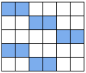
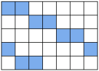
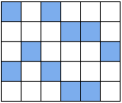
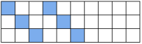
​​ (a) (b) (c) (d)

Figure 1: The random sampling pattern $\mathbf{q}^{t}=(q_{i}^{t})_{i=1}^{n}\in\mathbb{R}^{d\times n}$ used for communication is generated by a random permutation of the columns of a fixed binary template pattern, which has the prescribed number $s\geq 2$ of ones in every row. In (a) with $(d,n,s)=(5,6,2)$ and (b) with $(d,n,s)=(5,7,2)$, with ones in blue and zeros in white, examples of the template pattern used when $d\geq\frac{n}{s}$: for every row $k\in[d]$, there are $s$ ones at columns $i=\mathrm{mod}(s(k-1),n)+1,\ldots,\mathrm{mod}(sk-1,n)+1$. Thus, there are $\lfloor\frac{sd}{n}\rfloor$ or $\lceil\frac{sd}{n}\rceil$ ones in every column vector $q_{i}$. In (c), an example of sampling pattern obtained after a permutation of the columns of the template pattern in (a). In (d) with $(d,n,s)=(3,10,2)$, an example of the template pattern used when $\frac{n}{s}\geq d$: for every column $i=1,\ldots,ds$, there is 1 one at row $k=\mathrm{mod}(i-1,d)+1$. Thus, there is 0 or 1 one in every column vector $q_{i}$. We can note that when $d=\frac{n}{s}$, the two different rules for $d\geq\frac{n}{s}$ and $\frac{n}{s}\geq d$ for constructing the template pattern are equivalent, since they give exactly the same set of sampling patterns when permuting their columns. These two rules make it possible to generate easily the columns $q_{i}^{t}$ of $\mathbf{q}^{t}$ on the fly, without having to generate the whole mask $\mathbf{q}^{t}$ explicitly.

Our main result, stating linear convergence of CompressedScaffnew to the exact solution $x^{\star}$ of (1), is the following:

Theorem 3.1.

In CompressedScaffnew, suppose that

$$0<\gamma<\frac{2}{L}\quad\mbox{and}\quad 0<\eta\leq\frac{n(s-1)}{s(n-1)}\in\left(\frac{1}{2},1\right].$$ (3)

For every $t\geq 0$, define the Lyapunov function

$$\Psi^{t}\coloneqq\frac{1}{\gamma}\sum_{i=1}^{n}\left\|x_{i}^{t}-x^{\star}\right\|^{2}+\frac{\gamma}{p^{2}\eta}\frac{n-1}{s-1}\sum_{i=1}^{n}\left\|h_{i}^{t}-h_{i}^{\star}\right\|^{2},$$ (4)

where $x^{\star}$ is the unique solution to (1) and $h_{i}^{\star}=\nabla f_{i}(x^{\star})$. Then CompressedScaffnew converges linearly: for every $t\geq 0$,

$$\mathbb{E}\!\left[\Psi^{t}\right]\leq\rho^{t}\Psi^{0},$$ (5)

where

$$\rho\coloneqq\max\left((1-\gamma\mu)^{2},(\gamma L-1)^{2},1-p^{2}\eta\frac{s-1}{n-1}\right)<1.$$ (6)

Also, for every $i\in[n]$, $(x_{i}^{t})_{t\in\mathbb{N}}$ and $(\hat{x}_{i}^{t})_{t\in\mathbb{N}}$ both converge to $x^{\star}$ and $(h_{i}^{t})_{t\in\mathbb{N}}$ converges to $h_{i}^{\star}$, almost surely.

Remark 3.2.

One can simply set $\eta=\frac{1}{2}$ in CompressedScaffnew, which is independent of $n$ and $s$. However, the larger $\eta$, the better, so it is recommended to set

$$\eta=\frac{n(s-1)}{s(n-1)}.$$ (7)

3.1 Iteration complexity

CompressedScaffnew has the same iteration complexity as GD, with rate $\rho^{\sharp}\coloneqq\max(1-\gamma\mu,\gamma L-1)^{2}$, as long as $p$ and $s$ are large enough to have

$$1-p^{2}\eta\frac{s-1}{n-1}\leq\rho^{\sharp}.$$

This is remarkable: compression during aggregation with $p<1$ and $s<n$ does not harm convergence at all, until some threshold. This is in contrast with other algorithms with CC, like DIANA, where even a small amount of compression worsens the worst-case complexity.

For any $s\geq 2$, $p\in(0,1]$, $\gamma=\Theta(\frac{1}{L})$, and fixed $\eta\in(0,1]$, the asymptotic iteration complexity of CompressedScaffnew to reach $\epsilon$-accuracy, i.e. $\mathbb{E}\!\left[\Psi^{t}\right]\leq\epsilon$, is

$$\mathcal{O}\left(\left(\kappa+\frac{n}{sp^{2}}\right)\log\!\big{(}\epsilon^{-1}\big{)}\right).$$ (8)

Thus, by choosing

$$p=\min\left(\sqrt{\frac{(1-\rho^{\sharp})(n-1)}{\eta(s-1)}},1\right),$$ (9)

or more generally

$$p=\min\left(\Theta\left(\sqrt{\frac{n}{s\kappa}}\right),1\right),$$ (10)

the iteration complexity becomes

$$\mathcal{O}\left(\left(\kappa+\frac{n}{s}\right)\log\!\big{(}\epsilon^{-1}\big{)}\right).$$

In particular, with the choice recommended in (14) of $s=\max(2,\lfloor\frac{n}{d}\rfloor,\lfloor cn\rfloor)$, which yields the best TotalCom complexity, the iteration complexity is

$$\mathcal{O}\Big{(}\Big{(}\kappa+\min\!\big{(}d,n,{\textstyle\frac{1}{c}}\big{)}\Big{)}\log\!\big{(}\epsilon^{-1}\big{)}\Big{)}$$

(with $\frac{1}{c}=+\infty$ if $c=0$).

3.2 Convergence in the convex case

In this section only, we remove the hypothesis of strong convexity: the functions $f_{i}$ are just assumed to be convex and $L$-smooth, and we suppose that a solution $x^{\star}\in\mathbb{R}^{d}$ to (1) exists. Then we have sublinear ergodic convergence:

Theorem 3.3.

In CompressedScaffnew, suppose that

$$0<\gamma<\frac{2}{L}\quad\mbox{and}\quad 0<\eta<\frac{n(s-1)}{s(n-1)}\in\left(\frac{1}{2},1\right].$$ (11)

For every $i=1,\ldots,n$ and $T\geq 0$, we define

$$\tilde{x}_{i}^{T}\coloneqq\frac{1}{T+1}\sum_{t=0}^{T}x_{i}^{t}.$$ (12)

Then

$$\mathbb{E}\!\left[\left\|\nabla f(\tilde{x}_{i}^{T})\right\|^{2}\right]=\mathcal{O}\left(\frac{1}{T}\right)$$ (13)

(an explicit upper bound is given in the proof).

4 Communication complexity

For any $s\geq 2$, $p\in(0,1]$, $\gamma=\Theta(\frac{1}{L})$, and fixed $\eta\in(0,1]$, the asymptotic iteration complexity of CompressedScaffnew is given in (8). Communication occurs at every iteration with probability $p$, and during every communication round, DownCom consists in broadcasting the full $d$-dimensional vector $\bar{x}^{t}$, whereas in UpCom, compression is effective and the number of real values sent in parallel by the clients is equal to the number of ones per column in the sampling pattern $q$, which is $\lceil\frac{sd}{n}\rceil\geq 1$. Hence, the communication complexities are:

$$\mbox{DownCom:}\quad\mathcal{O}\left(pd\left(\kappa+\frac{n}{sp^{2}}\right)\log\!\big{(}\epsilon^{-1}\big{)}\right)\!,$$

$$\mbox{UpCom:}\quad\mathcal{O}\left(p\left(\frac{sd}{n}+1\right)\left(\kappa+\frac{n}{sp^{2}}\right)\log\!\big{(}\epsilon^{-1}\big{)}\right)\!.$$

$$\mbox{TotalCom:}\ \ \mathcal{O}\left(p\left(\frac{sd}{n}+1+cd\right)\left(\kappa+\frac{n}{sp^{2}}\right)\log\!\big{(}\epsilon^{-1}\big{)}\right)\!.$$

For a given $s$, the best choice for $p$, for both DownCom and UpCom, is given in (9), or more generally (10), for which

$$\mathcal{O}\left(p\left(\kappa+\frac{n}{sp^{2}}\right)\right)=\mathcal{O}\left(\sqrt{\frac{n\kappa}{s}}+\frac{n}{s}\right)$$

and the TotalCom complexity is

$$\mbox{TotalCom:}\ \ \mathcal{O}\left(\!\left(\sqrt{\frac{n\kappa}{s}}+\frac{n}{s}\right)\!\left(\frac{sd}{n}+1+cd\right)\log\!\big{(}\epsilon^{-1}\big{)}\!\right)\!.$$

We see the first acceleration effect due to LT: with a suitable $p<1$, the communication complexity only depends on $\sqrt{\kappa}$, not $\kappa$, whatever the compression level $s$. Without compression, i.e. $s=n$, CompressedScaffnew reverts to Scaffnew, with TotalCom complexity $\mathcal{O}\big{(}d\sqrt{\kappa}\log(\epsilon^{-1})\big{)}$. We can now set $s$ to further accelerate the algorithm, by minimizing the TotalCom complexity:

Theorem 4.1.

In CompressedScaffnew, suppose that (3) holds, with $\eta$ fixed and $\gamma=\Theta(\frac{1}{L})$, that $p$ satisfies (10) and that

$$s=\max\left(2,\left\lfloor\frac{n}{d}\right\rfloor,\lfloor cn\rfloor\right).$$ (14)

Then the TotalCom complexity of CompressedScaffnew is

$$\mathcal{O}\!\left(\left(d\frac{\sqrt{\kappa}}{\sqrt{n}}+\sqrt{d}\sqrt{\kappa}+d+\sqrt{c}\,d\sqrt{\kappa}\right)\log\!\big{(}\epsilon^{-1}\big{)}\right)\!.$$ (15)

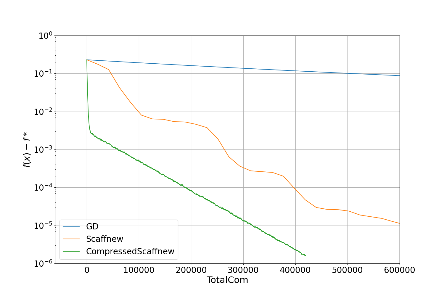
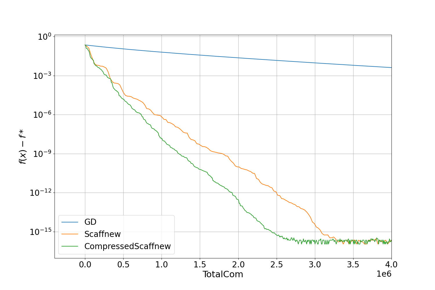
(a) real-sim, $n=2000$, $c=0$	(b) real-sim, $n=2000$, $c=0.2$
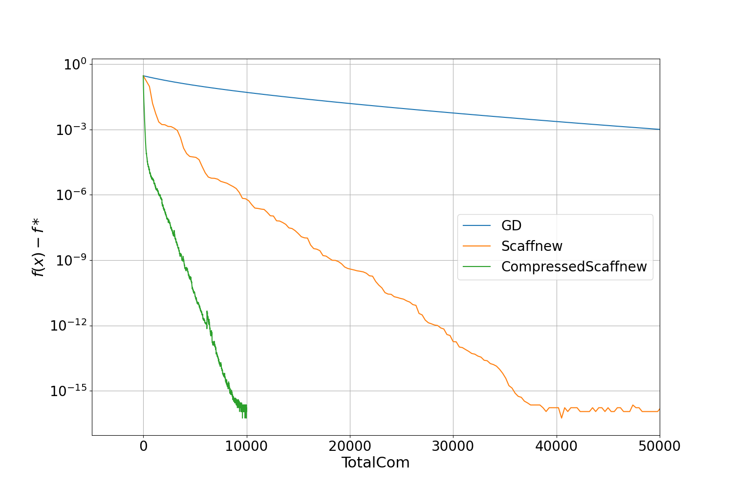
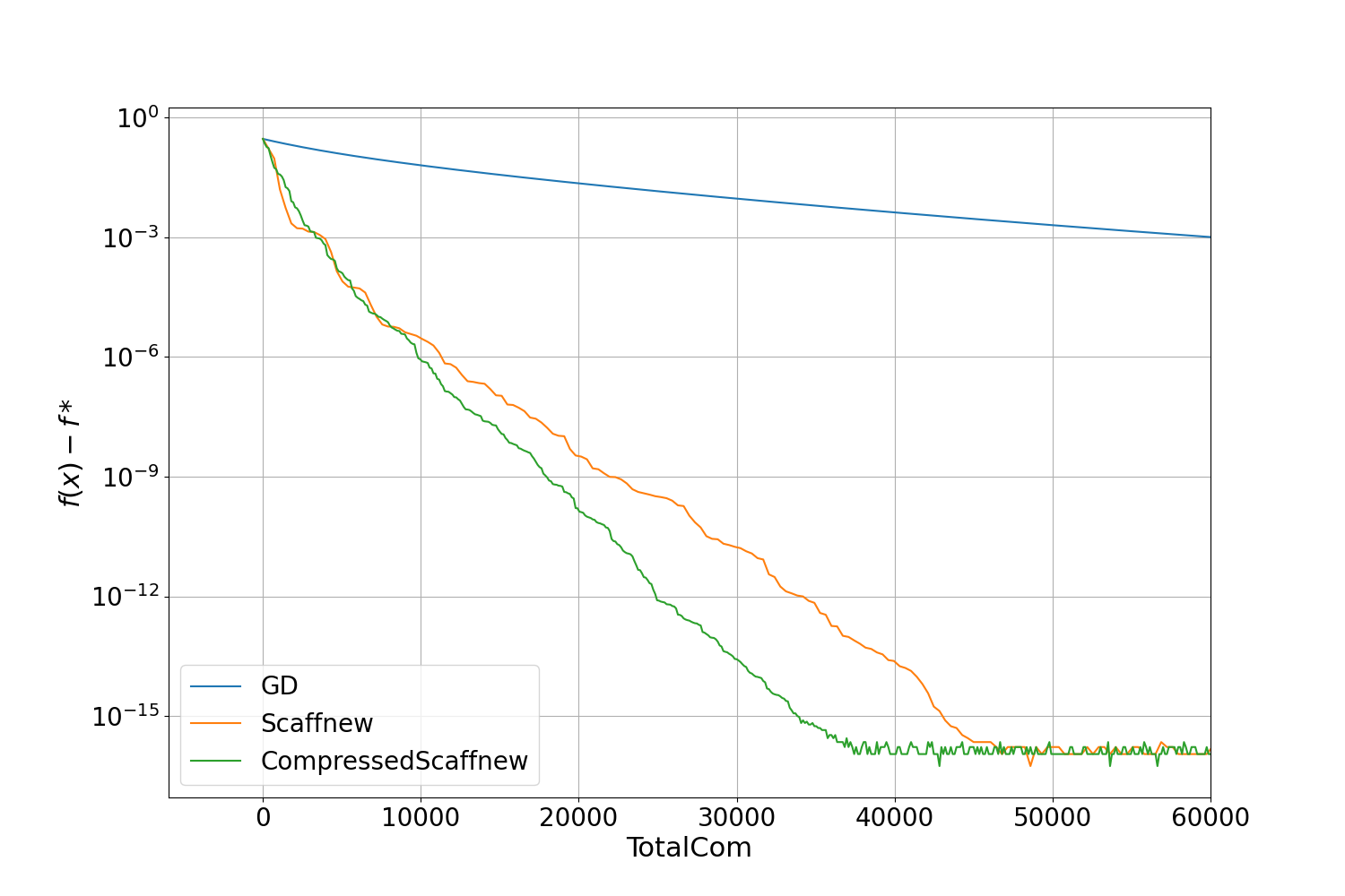
(c) w8a, $n=3000$, $c=0$	(d) w8a, $n=3000$, $c=0.2$

Figure 2: Logistic regression experiment. The datasets real-sim and w8a have $d=20,958$ and $d=300$ features, respectively. In (a) and (b), $d\approx 10n$, whereas in (c) and (d), this is the opposite with $n=10d$.

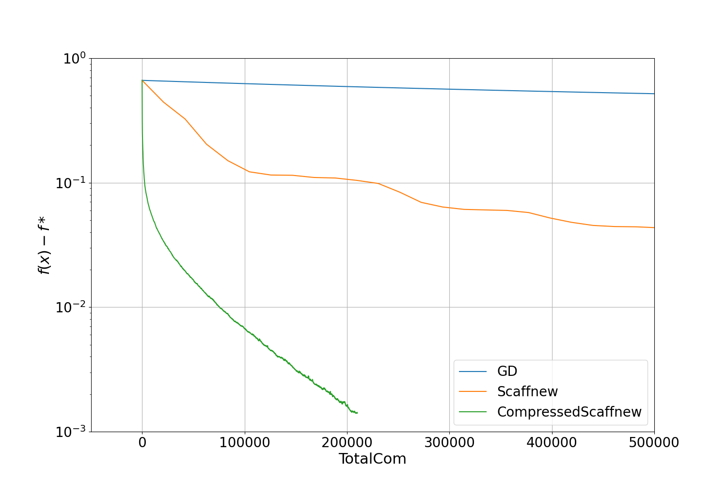
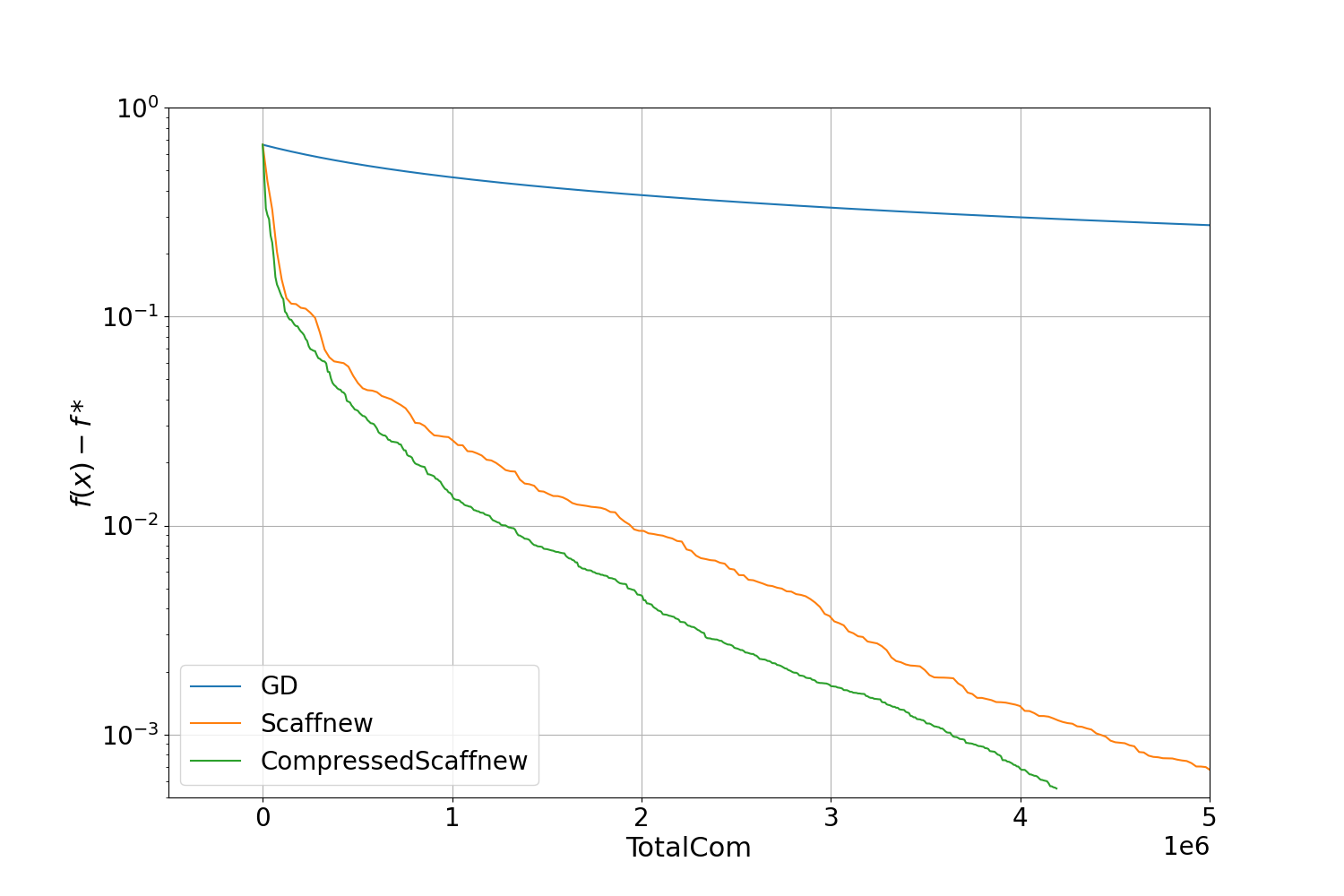
(a) real-sim, $n=2000$, $c=0$	(b) real-sim, $n=2000$, $c=0.2$
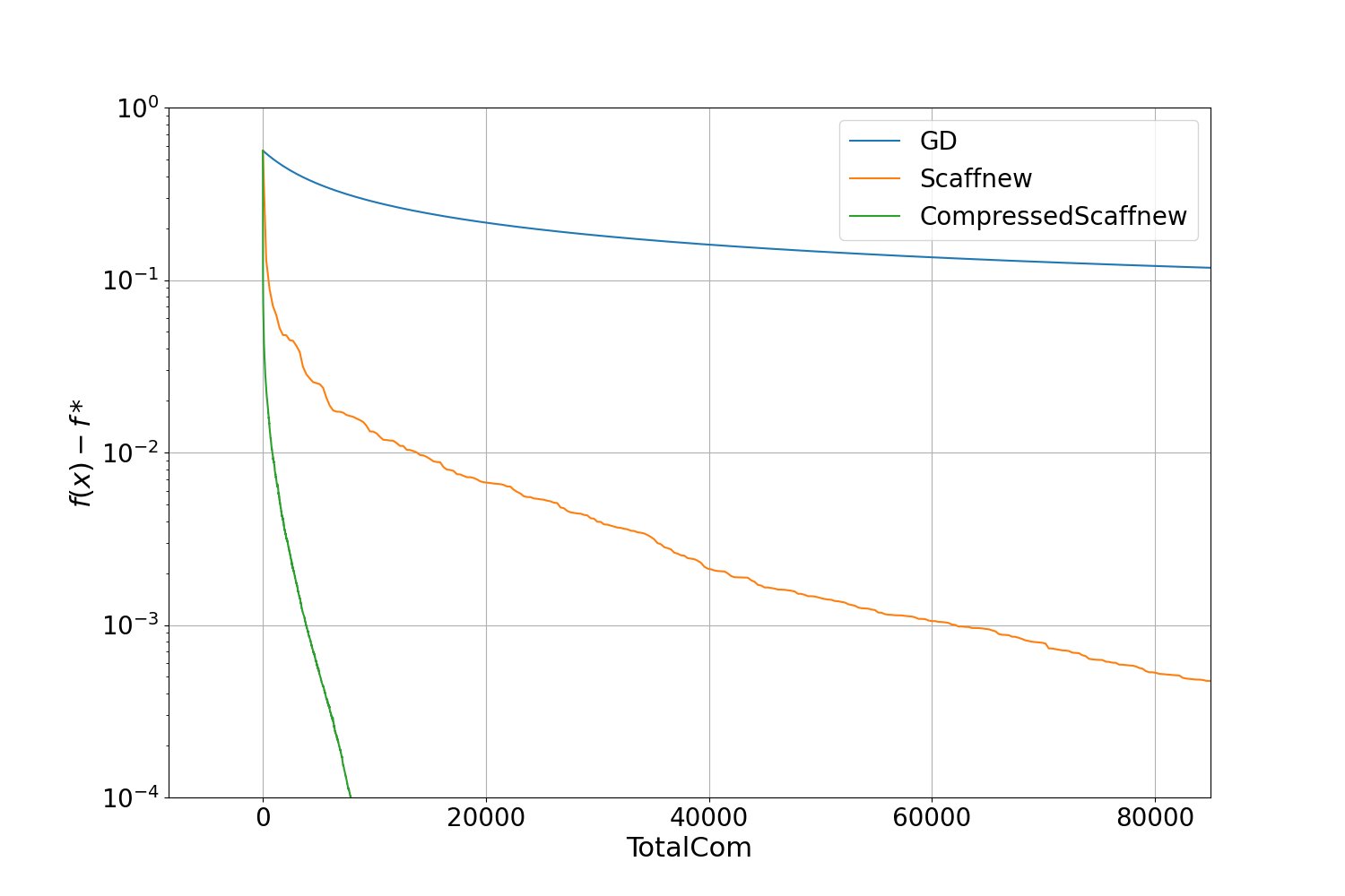
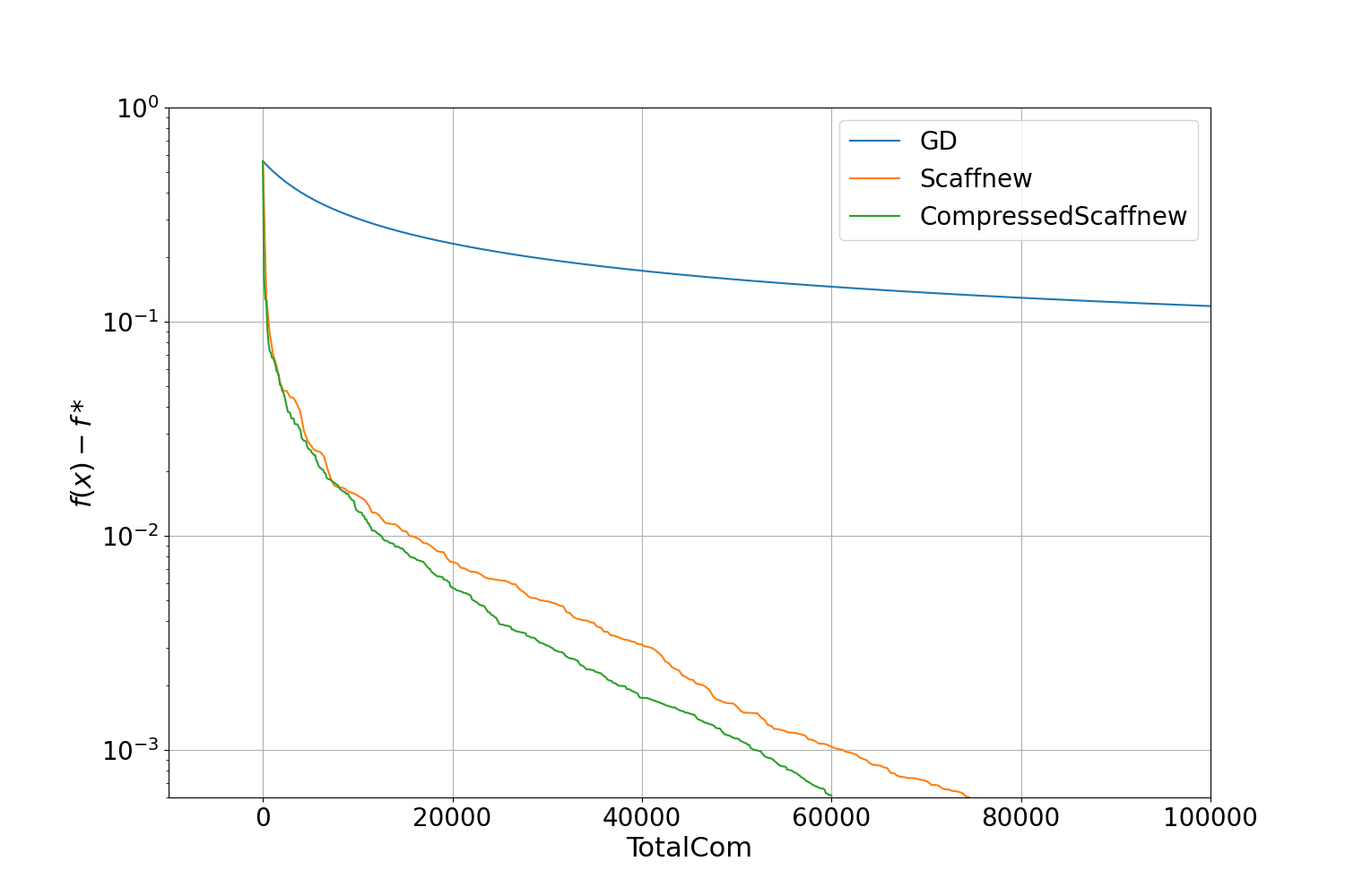
(c) w8a, $n=3000$, $c=0$	(d) w8a, $n=3000$, $c=0.2$

Figure 3: Logistic regression experiment. The setting is the same as in Figure 2, but with $\kappa=10^{6}$ instead of $334$.

Hence, as long as $c\leq\max(\frac{2}{n},\frac{1}{d},\frac{1}{\kappa})$, there is no difference with the case $c=0$, in which we only focus on UpCom, and the TotalCom complexity is

$$\mathcal{O}\!\left(\left(d\frac{\sqrt{\kappa}}{\sqrt{n}}+\sqrt{d}\sqrt{\kappa}+d\right)\log\!\big{(}\epsilon^{-1}\big{)}\right)\!.$$

On the other hand, if $c\geq\max(\frac{2}{n},\frac{1}{d},\frac{1}{\kappa})$, the complexity increases and becomes

$$\mathcal{O}\Big{(}\sqrt{c}\,d\sqrt{\kappa}\log\!\big{(}\epsilon^{-1}\big{)}\Big{)},$$

but compression remains operational and effective with the $\sqrt{c}$ factor. It is only when $c=1$ that $s=n$, i.e. there is no compression and CompressedScaffnew reverts to Scaffnew, and that the Upcom, DownCom and TotalCom complexities all become

$$\mathcal{O}\Big{(}d\sqrt{\kappa}\log\!\big{(}\epsilon^{-1}\big{)}\Big{)}.$$

In any case, for every $c\in[0,1]$, CompressedScaffnew is faster than Scaffnew.

We have reported in Table 1 the TotalCom complexity for several algorithms, and to the best of our knowledge, CompressedScaffnew improves upon all known algorithms, which use either LT or CC on top of GD.

5 Experiments

Carrying out large-scale experiments is beyond the scope of this work, which limits itself to foundational algorithmic and theoretical properties of above-mentioned algorithms. Nevertheless, we illustrate and confirm our results on a practical logistic regression problem.

The global loss function is

$$f(x)=\frac{1}{M}\sum_{m=1}^{M}\log(1+\exp(-b_{m}a_{m}^{\top}x))+\frac{\mu}{2}\|x\|^{2},$$ (16)

where the $a_{m}\in\mathbb{R}^{d}$ and $b_{m}\in\{-1,1\}$ are data samples and $M$ is their total number. The function $f$ in (16) is split into $n$ functions $f_{i}$ (the remainder of $M$ divided by $n$ samples is discarded). The strong convexity parameter $\mu$ is set to $0.003L_{0}$ in Figure 2 and $10^{-6}L_{0}$ in Figure 3, where $L_{0}$ is the smoothness constant without the $\frac{\mu}{2}\|x\|^{2}$ term (so that $L=L_{0}+\mu)$. We consider the case where the number of clients is larger than the model dimension ($n>d$) and vice versa. For this, we use the ‘w8a’ and ‘real-sim’ datasets from the classical LIBSVM library (Chang and Lin,, 2011). For each of them, we consider the two cases $c=0$ and $c=0.2$.

We measure the convergence error $f(x)-f(x^{\star})$ with respect to the TotalCom amount of communication, where $x$ is $x^{t}$ for GD and $\bar{x}^{t}$ when communication occurs for CompressedScaffnew and Scaffnew. The objective gap $f(x)-f(x^{\star})$ is a fair way to compare different algorithms and, since $f$ is $L$-smooth, $f(x)-f(x^{\star})\leq\frac{L}{2}\|x-x^{\star}\|^{2}$ for any $x$, so that it is guaranteed to converge linearly with the same rate as $\Psi$ in Theorem 3.1.

The stepsize $\gamma=\frac{2}{L+\mu}$ is used in all algorithms. The probability $p$ is set to $\frac{1}{\sqrt{\kappa}}$ for Scaffnew and $\min(\sqrt{\frac{n}{s\kappa}},1)$ for CompressedScaffnew, with $s$ and $\eta$ set according to Equations (14) and (7), respectively. $x^{0}$ and the $h_{i}^{0}$ are all set to zero vectors.

The results are shown in Figures 2 and 3. The algorithms converge linearly, and CompressedScaffnew is faster than Scaffnew, as expected. This confirms that the proposed compression technique is effective. The speedup of CompressedScaffnew over Scaffnew is higher for $c=0$ than for $c=0.2$. This is also expected, since when $c$ increases, there is less compression and the two algorithms become more similar; they are the same, without compression, when $c=1$.

6 Conclusion

Our proposed algorithm CompressedScaffnew is the first to provably benefit from the two combined acceleration mechanisms of Local Training (LT) and Communication Compression (CC). Moreover, this is achieved not only for uplink communication, but for our more comprehensive model of total communication. Our theoretical achievements are confirmed in practice. This pushes the boundary of our understanding of LT and CC to a new level. Among venues for future work, we can mention replacing the true gradients $\nabla f_{i}$ by stochastic estimates, a feature present in several algorithms like Scaffnew (Malinovsky et al.,, 2022) and FedCOMGATE (Haddadpour et al.,, 2021), or allowing for partial participation and for a larger class of possibly biased compressors, including quantization. The nonconvex case should also be studied (Karimireddy et al.,, 2021; Das et al.,, 2022).

Appendix

Appendix A Proof of Theorem 3.1

We introduce vector notations to simplify the derivations: the problem (1) can be written as

$$\mathrm{find}\ \mathbf{x}^{\star}=\operatorname*{arg\,min}_{\mathbf{x}\in\mathcal{X}}\ \mathbf{f}(\mathbf{x})\quad\mbox{s.t.}\quad W\mathbf{x}=0,$$ (17)

where $\mathcal{X}\coloneqq\mathbb{R}^{d\times n}$, an element $\mathbf{x}=(x_{i})_{i=1}^{n}\in\mathcal{X}$ is a collection of vectors $x_{i}\in\mathbb{R}^{d}$, $\mathbf{f}:\mathbf{x}\in\mathcal{X}\mapsto\sum_{i=1}^{n}f_{i}(x_{i})$ is $L$-smooth and $\mu$-strongly convex, the linear operator $W:\mathcal{X}\rightarrow\mathcal{X}$ maps $\mathbf{x}=(x_{i})_{i=1}^{n}$ to $(x_{i}-\frac{1}{n}\sum_{j=1}^{n}x_{j})_{i=1}^{n}$. The constraint $W\mathbf{x}=0$ means that $\mathbf{x}$ minus its average is zero; that is, $\mathbf{x}$ has identical components $x_{1}=\cdots=x_{n}$. Thus, (17) is indeed equivalent to (1). We have $W=W^{*}=W^{2}$.

We solve the problem (17) using the following algorithm, which will be shown below to be CompressedScaffnew:

Algorithm 2

  input: stepsizes $\gamma>0$, $\tau>0$; $s\in\{2,\ldots,n\}$; initial estimates $\mathbf{x}^{0}\in\mathcal{X}$, $\mathbf{u}^{0}\in\mathcal{X}$ with $\sum_{i=1}^{n}u_{i}^{0}=0$; constant $\omega\geq 0$; sequence of independent coin flips $\theta^{0},\theta^{1},\ldots$ with $\mathrm{Prob}(\theta^{t}=1)=p$, and for every $t$ with $\theta^{t}=1$, a random binary mask $\mathbf{q}^{t}=(q_{i}^{t})_{i=1}^{n}\in\mathbb{R}^{d\times n}$ generated as explained in Figure 1. The compressed vector $\mathcal{C}^{t}_{i}(v)$ is $v$ multiplied elementwise by $q_{i}^{t}$.

  for $t=0,1,\ldots$ do

     $\mathbf{\hat{x}}^{t}\coloneqq\mathbf{x}^{t}-\gamma\nabla\mathbf{f}(\mathbf{x}^{t})-\gamma\mathbf{u}^{t}$

     if $\theta^{t}=1$ then

        $\bar{x}^{t}\coloneqq\frac{1}{s}\sum_{j=1}^{n}\mathcal{C}_{j}^{t}(\hat{x}_{j}^{t})$

        $\mathbf{x}^{t+1}\coloneqq\mathbf{\bar{x}}^{t}$, with $\bar{x}_{i}^{t}=\bar{x}^{t}$, for every $i=1,\ldots,n$

     else

        $\mathbf{x}^{t+1}\coloneqq\mathbf{\hat{x}}^{t}$

     end if

     $\mathbf{d}^{t}:\approx W\mathbf{\hat{x}}^{t}$

     $\mathbf{u}^{t+1}\coloneqq\mathbf{u}^{t}+\frac{\tau}{1+\omega}\mathbf{d}^{t}$

  end for

We denote by $\mathcal{F}_{t}$ the $\sigma$-algebra generated by the collection of $\mathcal{X}$-valued random variables $(\mathbf{x}^{0},\mathbf{u}^{0}),\ldots,(\mathbf{x}^{t},\mathbf{u}^{t})$, for every $t\geq 0$. In Algorithm 2, $\mathbf{d}^{t}:\approx W\mathbf{\hat{x}}^{t}$ means that $\mathbf{d}^{t}$ is a random variable with expectation $W\mathbf{\hat{x}}^{t}$. Its construction, so that Algorithm 2 becomes CompressedScaffnew, is explained in Section A.1, but the convergence analysis of Algorithm 2 only relies on the 3 following properties of this stochastic process, which are supposed to hold: for every $t\geq 0$,

1. $\mathbb{E}\!\left[\mathbf{d}^{t}\;|\;\mathcal{F}^{t}\right]=W\mathbf{\hat{x}}^{t}$.

2. There exists a value $\omega\geq 0$ such that

   $$\mathbb{E}\!\left[\left\|\mathbf{d}^{t}-W\mathbf{\hat{x}}^{t}\right\|^{2}\;|\;\mathcal{F}^{t}\right]\leq\omega\left\|W\mathbf{\hat{x}}^{t}\right\|^{2}.$$ (18)

3. $\mathbf{d}^{t}$ belongs to the range of $W$; that is, $\sum_{i=1}^{n}d^{t}_{i}=0$.

In Algorithm 2, we suppose that $\sum_{i=1}^{n}u^{0}_{i}=0$. Then, it follows from the third property of $\mathbf{d}^{t}$ that, for every $t\geq 0$, $\sum_{i=1}^{n}u^{t}_{i}=0$; that is, $W\mathbf{u}^{t}=\mathbf{u}^{t}$.

Algorithm 2 converges linearly:

Theorem A.1.

In Algorithm 2, suppose that $0<\gamma<\frac{2}{L}$ and that $\tau\leq\frac{p}{\gamma}\frac{n(s-1)}{s(n-1)}$. For every $t\geq 0$, define the Lyapunov function

$$\Psi^{t}\coloneqq\frac{1}{\gamma}\left\|\mathbf{x}^{t}-\mathbf{x}^{\star}\right\|^{2}+\frac{1+\omega}{\tau}\left\|\mathbf{u}^{t}-\mathbf{u}^{\star}\right\|^{2},$$ (19)

where $\mathbf{x}^{\star}$ is the unique solution to (17) and $\mathbf{u}^{\star}\coloneqq-\nabla\mathbf{f}(\mathbf{x}^{\star})$. Then Algorithm 2 converges linearly: for every $t\geq 0$,

$$\mathbb{E}\!\left[\Psi^{t}\right]\leq\rho^{t}\Psi^{0},$$ (20)

where

$$\rho\coloneqq\max\left((1-\gamma\mu)^{2},(\gamma L-1)^{2},1-\frac{\gamma\tau}{1+\omega}\right)<1.$$ (21)

Also, $(\mathbf{x}^{t})_{t\in\mathbb{N}}$ and $(\mathbf{\hat{x}}^{t})_{t\in\mathbb{N}}$ both converge to $\mathbf{x}^{\star}$ and $(\mathbf{u}^{t})_{t\in\mathbb{N}}$ converges to $\mathbf{u}^{\star}$, almost surely.

Proof.

For every $t\geq 0$, we define $\mathbf{\hat{u}}^{t+1}\coloneqq\mathbf{u}^{t}+\tau W\mathbf{\hat{x}}^{t}$, $\mathbf{w}^{t}\coloneqq\mathbf{x}^{t}-\gamma\nabla\mathbf{f}(\mathbf{x}^{t})$ and $\mathbf{w}^{\star}\coloneqq\mathbf{x}^{\star}-\gamma\nabla\mathbf{f}(\mathbf{x}^{\star})$. We also define $\mathbf{\bar{x}}^{t\sharp}\coloneqq(\bar{x}^{t\sharp})_{i=1}^{n}$, with $\bar{x}^{t\sharp}\coloneqq\frac{1}{n}\sum_{i=1}^{n}\hat{x}_{i}^{t}$; that is, $\bar{x}^{t\sharp}$ is the exact average of the $\hat{x}_{i}^{t}$, of which $\bar{x}^{t}$ is an unbiased random estimate.

We have

$$\mathbb{E}\!\left[\left\|\mathbf{x}^{t+1}-\mathbf{x}^{\star}\right\|^{2}\;|\;\mathcal{F}_{t}\right] =p\mathbb{E}_{\mathbf{q}^{t}}\!\left[\left\|\mathbf{\bar{x}}^{t}-\mathbf{x}^{\star}\right\|^{2}\;|\;\mathcal{F}_{t}\right]+(1-p)\left\|\mathbf{\hat{x}}^{t}-\mathbf{x}^{\star}\right\|^{2},$$

where $\mathbb{E}_{\mathbf{q}^{t}}$ denotes the expectation with respect to the random mask $\mathbf{q}^{t}$. To analyze $\mathbb{E}_{\mathbf{q}^{t}}\!\left[\left\|\mathbf{\bar{x}}^{t}-\mathbf{x}^{\star}\right\|^{2}\;|\;\mathcal{F}_{t}\right]$, we can remark that the expectation and the squared Euclidean norm are separable with respect to the coordinates of the $d$-dimensional vectors, so that we can reason on the coordinates independently on each other, even if the the coordinates, or rows, of $\mathbf{q}^{t}$ are mutually dependent. Thus, for every coordinate $k\in[d]$, it is like a subset $\Omega_{k}^{t}\subset[n]$ of size $s$, which corresponds to the location of the ones in the $k$-th row of $\mathbf{q}^{t}$, is chosen uniformly at random and

$$\bar{x}^{t}_{k}=\frac{1}{s}\sum_{i\in\Omega_{k}^{t}}\hat{x}_{i,k}^{t}.$$

Since $\mathbb{E}_{\mathbf{q}^{t}}\!\left[\mathbf{\bar{x}}^{t}\;|\;\mathcal{F}_{t}\right]=\mathbf{\bar{x}}^{t\sharp}$,

$$\mathbb{E}_{\mathbf{q}^{t}}\!\left[\left\|\mathbf{\bar{x}}^{t}-\mathbf{x}^{\star}\right\|^{2}\;|\;\mathcal{F}_{t}\right] =\left\|\mathbf{\bar{x}}^{t\sharp}-\mathbf{x}^{\star}\right\|^{2}+\mathbb{E}_{\mathbf{q}^{t}}\!\left[\left\|\mathbf{\bar{x}}^{t}-\mathbf{\bar{x}}^{t\sharp}\right\|^{2}\;|\;\mathcal{F}_{t}\right],$$

with

$$\left\|\mathbf{\bar{x}}^{t\sharp}-\mathbf{x}^{\star}\right\|^{2}=\left\|\mathbf{\hat{x}}^{t}-\mathbf{x}^{\star}\right\|^{2}-\left\|W\mathbf{\hat{x}}^{t}\right\|^{2}$$

and, as proved in Condat and Richtárik, (2022, Proposition 1),

$$\mathbb{E}_{\mathbf{q}^{t}}\!\left[\left\|\mathbf{\bar{x}}^{t}-\mathbf{\bar{x}}^{t\sharp}\right\|^{2}\;|\;\mathcal{F}_{t}\right]=n\sum_{k=1}^{d}\mathbb{E}_{\Omega_{k}^{t}}\!\left[\left(\frac{1}{s}\sum_{i\in\Omega_{k}^{t}}\hat{x}_{i,k}^{t}-\frac{1}{n}\sum_{j=1}^{n}\hat{x}_{j,k}^{t}\right)^{2}\;|\;\mathcal{F}_{t}\right]=\nu\left\|W\mathbf{\hat{x}}^{t}\right\|^{2},$$

where

$$\nu\coloneqq\frac{n-s}{s(n-1)}\in\left[0,\frac{1}{2}\right).$$ (22)

Moreover,

$$\left\|\mathbf{\hat{x}}^{t}-\mathbf{x}^{\star}\right\|^{2} =\left\|\mathbf{w}^{t}-\mathbf{w}^{\star}\right\|^{2}+\gamma^{2}\left\|\mathbf{u}^{t}-\mathbf{u}^{\star}\right\|^{2}-2\gamma\langle\mathbf{w}^{t}-\mathbf{w}^{\star},\mathbf{u}^{t}-\mathbf{u}^{\star}\rangle$$

$$=\left\|\mathbf{w}^{t}-\mathbf{w}^{\star}\right\|^{2}-\gamma^{2}\left\|\mathbf{u}^{t}-\mathbf{u}^{\star}\right\|^{2}-2\gamma\langle\mathbf{\hat{x}}^{t}-\mathbf{x}^{\star},\mathbf{u}^{t}-\mathbf{u}^{\star}\rangle$$

$$=\left\|\mathbf{w}^{t}-\mathbf{w}^{\star}\right\|^{2}-\gamma^{2}\left\|\mathbf{u}^{t}-\mathbf{u}^{\star}\right\|^{2}-2\gamma\langle\mathbf{\hat{x}}^{t}-\mathbf{x}^{\star},\mathbf{\hat{u}}^{t+1}-\mathbf{u}^{\star}\rangle+2\gamma\langle\mathbf{\hat{x}}^{t}-\mathbf{x}^{\star},\mathbf{\hat{u}}^{t+1}-\mathbf{u}^{t}\rangle$$

$$=\left\|\mathbf{w}^{t}-\mathbf{w}^{\star}\right\|^{2}-\gamma^{2}\left\|\mathbf{u}^{t}-\mathbf{u}^{\star}\right\|^{2}-2\gamma\langle\mathbf{\hat{x}}^{t}-\mathbf{x}^{\star},\mathbf{\hat{u}}^{t+1}-\mathbf{u}^{\star}\rangle+2\gamma\tau\langle\mathbf{\hat{x}}^{t}-\mathbf{x}^{\star},W\mathbf{\hat{x}}^{t}\rangle$$

$$=\left\|\mathbf{w}^{t}-\mathbf{w}^{\star}\right\|^{2}-\gamma^{2}\left\|\mathbf{u}^{t}-\mathbf{u}^{\star}\right\|^{2}-2\gamma\langle\mathbf{\hat{x}}^{t}-\mathbf{x}^{\star},\mathbf{\hat{u}}^{t+1}-\mathbf{u}^{\star}\rangle+2\gamma\tau\left\|W\mathbf{\hat{x}}^{t}\right\|^{2}.$$

Hence,

$$\mathbb{E}\!\left[\left\|\mathbf{x}^{t+1}-\mathbf{x}^{\star}\right\|^{2}\;|\;\mathcal{F}_{t}\right] =p\left\|\mathbf{\hat{x}}^{t}-\mathbf{x}^{\star}\right\|^{2}-p\left\|W\mathbf{\hat{x}}^{t}\right\|^{2}+p\nu\left\|W\mathbf{\hat{x}}^{t}\right\|^{2}+(1-p)\left\|\mathbf{\hat{x}}^{t}-\mathbf{x}^{\star}\right\|^{2}$$

$$=\left\|\mathbf{\hat{x}}^{t}-\mathbf{x}^{\star}\right\|^{2}-p(1-\nu)\left\|W\mathbf{\hat{x}}^{t}\right\|^{2}$$

$$=\left\|\mathbf{w}^{t}-\mathbf{w}^{\star}\right\|^{2}-\gamma^{2}\left\|\mathbf{u}^{t}-\mathbf{u}^{\star}\right\|^{2}-2\gamma\langle\mathbf{\hat{x}}^{t}-\mathbf{x}^{\star},\mathbf{\hat{u}}^{t+1}-\mathbf{u}^{\star}\rangle$$

$$\quad+\big{(}2\gamma\tau-p(1-\nu)\big{)}\left\|W\mathbf{\hat{x}}^{t}\right\|^{2}.$$

On the other hand,

$$\mathbb{E}\!\left[\left\|\mathbf{u}^{t+1}-\mathbf{u}^{\star}\right\|^{2}\;|\;\mathcal{F}_{t}\right] \leq\left\|\mathbf{u}^{t}-\mathbf{u}^{\star}+\frac{1}{1+\omega}\big{(}\mathbf{\hat{u}}^{t+1}-\mathbf{u}^{t}\big{)}\right\|^{2}+\frac{\omega}{(1+\omega)^{2}}\left\|\mathbf{\hat{u}}^{t+1}-\mathbf{u}^{t}\right\|^{2}$$

$$=\left\|\frac{\omega}{1+\omega}\big{(}\mathbf{u}^{t}-\mathbf{u}^{\star}\big{)}+\frac{1}{1+\omega}\big{(}\mathbf{\hat{u}}^{t+1}-\mathbf{u}^{\star}\big{)}\right\|^{2}+\frac{\omega}{(1+\omega)^{2}}\left\|\mathbf{\hat{u}}^{t+1}-\mathbf{u}^{t}\right\|^{2}$$

$$=\frac{\omega^{2}}{(1+\omega)^{2}}\left\|\mathbf{u}^{t}-\mathbf{u}^{\star}\right\|^{2}+\frac{1}{(1+\omega)^{2}}\left\|\mathbf{\hat{u}}^{t+1}-\mathbf{u}^{\star}\right\|^{2}$$

$$\quad+\frac{2\omega}{(1+\omega)^{2}}\langle\mathbf{u}^{t}-\mathbf{u}^{\star},\mathbf{\hat{u}}^{t+1}-\mathbf{u}^{\star}\rangle+\frac{\omega}{(1+\omega)^{2}}\left\|\mathbf{\hat{u}}^{t+1}-\mathbf{u}^{\star}\right\|^{2}$$

$$\quad+\frac{\omega}{(1+\omega)^{2}}\left\|\mathbf{u}^{t}-\mathbf{u}^{\star}\right\|^{2}-\frac{2\omega}{(1+\omega)^{2}}\langle\mathbf{u}^{t}-\mathbf{u}^{\star},\mathbf{\hat{u}}^{t+1}-\mathbf{u}^{\star}\rangle$$

$$=\frac{1}{1+\omega}\left\|\mathbf{\hat{u}}^{t+1}-\mathbf{u}^{\star}\right\|^{2}+\frac{\omega}{1+\omega}\left\|\mathbf{u}^{t}-\mathbf{u}^{\star}\right\|^{2}.$$

Moreover,

$$\left\|\mathbf{\hat{u}}^{t+1}-\mathbf{u}^{\star}\right\|^{2} =\left\|(\mathbf{u}^{t}-\mathbf{u}^{\star})+(\mathbf{\hat{u}}^{t+1}-\mathbf{u}^{t})\right\|^{2}$$

$$=\left\|\mathbf{u}^{t}-\mathbf{u}^{\star}\right\|^{2}+\left\|\mathbf{\hat{u}}^{t+1}-\mathbf{u}^{t}\right\|^{2}+2\langle\mathbf{u}^{t}-\mathbf{u}^{\star},\mathbf{\hat{u}}^{t+1}-\mathbf{u}^{t}\rangle$$

$$=\left\|\mathbf{u}^{t}-\mathbf{u}^{\star}\right\|^{2}+2\langle\mathbf{\hat{u}}^{t+1}-\mathbf{u}^{\star},\mathbf{\hat{u}}^{t+1}-\mathbf{u}^{t}\rangle-\left\|\mathbf{\hat{u}}^{t+1}-\mathbf{u}^{t}\right\|^{2}$$

$$=\left\|\mathbf{u}^{t}-\mathbf{u}^{\star}\right\|^{2}-\left\|\mathbf{\hat{u}}^{t+1}-\mathbf{u}^{t}\right\|^{2}+2\tau\langle\mathbf{\hat{u}}^{t+1}-\mathbf{u}^{\star},W(\mathbf{\hat{x}}^{t}-\mathbf{x}^{\star})\rangle$$

$$=\left\|\mathbf{u}^{t}-\mathbf{u}^{\star}\right\|^{2}-\tau^{2}\left\|W\mathbf{\hat{x}}^{t}\right\|^{2}+2\tau\langle W(\mathbf{\hat{u}}^{t+1}-\mathbf{u}^{\star}),\mathbf{\hat{x}}^{t}-\mathbf{x}^{\star}\rangle$$

$$=\left\|\mathbf{u}^{t}-\mathbf{u}^{\star}\right\|^{2}-\tau^{2}\left\|W\mathbf{\hat{x}}^{t}\right\|^{2}+2\tau\langle\mathbf{\hat{u}}^{t+1}-\mathbf{u}^{\star},\mathbf{\hat{x}}^{t}-\mathbf{x}^{\star}\rangle.$$

Hence,

$$\frac{1}{\gamma}\mathbb{E}\!\left[\left\|\mathbf{x}^{t+1}-\mathbf{x}^{\star}\right\|^{2}\;|\;\mathcal{F}_{t}\right] +\frac{1+\omega}{\tau}\mathbb{E}\!\left[\left\|\mathbf{u}^{t+1}-\mathbf{u}^{\star}\right\|^{2}\;|\;\mathcal{F}_{t}\right]$$

$$\leq\frac{1}{\gamma}\left\|\mathbf{w}^{t}-\mathbf{w}^{\star}\right\|^{2}-\gamma\left\|\mathbf{u}^{t}-\mathbf{u}^{\star}\right\|^{2}+\left(2\tau-\frac{p}{\gamma}(1-\nu)\right)\left\|W\mathbf{\hat{x}}^{t}\right\|^{2}$$

$$\quad-2\langle\mathbf{\hat{x}}^{t}-\mathbf{x}^{\star},\mathbf{\hat{u}}^{t+1}-\mathbf{u}^{\star}\rangle+\frac{1}{\tau}\left\|\mathbf{u}^{t}-\mathbf{u}^{\star}\right\|^{2}$$

$$\quad-\tau\left\|W\mathbf{\hat{x}}^{t}\right\|^{2}+2\langle\mathbf{\hat{u}}^{t+1}-\mathbf{u}^{\star},\mathbf{\hat{x}}^{t}-\mathbf{x}^{\star}\rangle+\frac{\omega}{\tau}\left\|\mathbf{u}^{t}-\mathbf{u}^{\star}\right\|^{2}$$

$$=\frac{1}{\gamma}\left\|\mathbf{w}^{t}-\mathbf{w}^{\star}\right\|^{2}+\left(\frac{1+\omega}{\tau}-\gamma\right)\left\|\mathbf{u}^{t}-\mathbf{u}^{\star}\right\|^{2}$$

$$\quad+\left(\tau-\frac{p}{\gamma}(1-\nu)\right)\left\|W\mathbf{\hat{x}}^{t}\right\|^{2}.$$ (23)

Since we have supposed $\tau-\frac{p}{\gamma}(1-\nu)\leq 0$,

$$\frac{1}{\gamma}\mathbb{E}\!\left[\left\|\mathbf{x}^{t+1}-\mathbf{x}^{\star}\right\|^{2}\;|\;\mathcal{F}_{t}\right]+\frac{1+\omega}{\tau}\mathbb{E}\!\left[\left\|\mathbf{u}^{t+1}-\mathbf{u}^{\star}\right\|^{2}\;|\;\mathcal{F}_{t}\right]$$

$$\qquad\qquad\leq\frac{1}{\gamma}\left\|\mathbf{w}^{t}-\mathbf{w}^{\star}\right\|^{2}+\frac{1+\omega}{\tau}\left(1-\frac{\gamma\tau}{1+\omega}\right)\left\|\mathbf{u}^{t}-\mathbf{u}^{\star}\right\|^{2}.$$

According to Condat and Richtárik, (2022, Lemma 1),

$$\left\|\mathbf{w}^{t}-\mathbf{w}^{\star}\right\|^{2} =\left\|(\mathrm{Id}-\gamma\nabla\mathbf{f})\mathbf{x}^{t}-(\mathrm{Id}-\gamma\nabla\mathbf{f})\mathbf{x}^{\star}\right\|^{2}$$

$$\leq\max(1-\gamma\mu,\gamma L-1)^{2}\left\|\mathbf{x}^{t}-\mathbf{x}^{\star}\right\|^{2}.$$

Therefore,

$$\mathbb{E}\!\left[\Psi^{t+1}\;|\;\mathcal{F}_{t}\right] \leq\max\left((1-\gamma\mu)^{2},(\gamma L-1)^{2},1-\frac{\gamma\tau}{1+\omega}\right)\Psi^{t}.$$ (24)

Using the tower rule, we can unroll the recursion in (24) to obtain the unconditional expectation of $\Psi^{t+1}$. Moreover, using classical results on supermartingale convergence (Bertsekas,, 2015, Proposition A.4.5), it follows from (24) that $\Psi^{t}\rightarrow 0$ almost surely. Almost sure convergence of $\mathbf{x}^{t}$ and $\mathbf{u}^{t}$ follows. Finally, by Lipschitz continuity of $\nabla\mathbf{f}$, we can upper bound $\|\mathbf{\hat{x}}^{t}-\mathbf{x}^{\star}\|^{2}$ by a linear combination of $\|\mathbf{x}^{t}-\mathbf{x}^{\star}\|^{2}$ and $\|\mathbf{u}^{t}-\mathbf{u}^{\star}\|^{2}$. It follows that $\mathbb{E}\!\left[\left\|\mathbf{\hat{x}}^{t}-\mathbf{x}^{\star}\right\|^{2}\right]\rightarrow 0$ linearly with the same rate $\rho$ and that $\mathbf{\hat{x}}^{t}\rightarrow\mathbf{x}^{\star}$ almost surely, as well. ∎

CompressedScaffnew corresponds to Algorithm 2 with $u_{i}$ replaced by $-h_{i}$, the randomization strategy for the dual update detailed in Section A.1, the variance factors $\omega$ and $\nu$ defined in (27) and (22), respectively, and $\tau\coloneqq\frac{p}{\gamma}\eta$, for some $\eta$ with

$$0<\eta\leq 1-\nu=\frac{n(s-1)}{s(n-1)}\in\left(\frac{1}{2},1\right].$$

With these substitutions, Theorem A.1 yields Theorem 3.1.

A.1 The random variable $\mathbf{d}^{t}$

We define the random variable $\mathbf{d}^{t}$ used in Algorithm 2, so that it becomes CompressedScaffnew. If $\theta^{t}=0$, $\mathbf{d}^{t}\coloneqq 0$. If, on the other hand, $\theta^{t}=1$, for every coordinate $k\in[d]$, a subset $\Omega_{k}^{t}\subset[n]$ of size $s$ is chosen uniformly at random. These sets $(\Omega_{k}^{t})_{k=1}^{d}$ are mutually dependent, but this does not matter for the derivations, since we can reason on the coordinates separately. Then, for every $k\in[d]$ and $i\in[n]$,

$$d^{t}_{i,k}\coloneqq\left\{\begin{array}[]{l}a\left(\hat{x}_{i,k}^{t}-\frac{1}{s}\sum_{j\in\Omega_{k}^{t}}\hat{x}_{j,k}^{t}\right)\ \mbox{if }i\in\Omega_{k}^{t},\\ 0\ \mbox{otherwise},\end{array}\right.$$ (25)

for some value $a>0$ to determine. We can check that $\sum_{i=1}^{n}d^{t}_{i}=0$. We can also note that $\mathbf{d}^{t}$ depends only on $W\mathbf{\hat{x}}^{t}$ and not on $\mathbf{\hat{x}}^{t}$; in particular, if $\hat{x}_{1}^{t}=\cdots=\hat{x}_{n}^{t}$, $d_{i}^{t}=0$. We have to set $a$ so that $\mathbb{E}\!\left[d_{i}^{t}\right]=\hat{x}_{i}^{t}-\frac{1}{n}\sum_{j=1}^{n}\hat{x}_{j}^{t}$, where the expectation is with respect to $\theta^{t}$ and the $\Omega_{k}^{t}$ (all expectations in this section are conditional to $\mathbf{\hat{x}}^{t}$). So, let us calculate this expectation.

Let $k\in[d]$. For every $i\in[n]$,

$$\mathbb{E}\!\left[d^{t}_{i,k}\right]=p\frac{s}{n}\left(a\hat{x}_{i,k}^{t}-\frac{a}{s}\mathbb{E}_{\Omega:i\in\Omega}\!\left[\sum_{j\in\Omega}\hat{x}_{j,k}^{t}\right]\right),$$

where $\mathbb{E}_{\Omega:i\in\Omega}$ denotes the expectation with respect to a subset $\Omega\subset[n]$ of size $s$ containing $i$ and chosen uniformly at random. We have

$$\mathbb{E}_{\Omega:i\in\Omega}\!\left[\sum_{j\in\Omega}\hat{x}_{j,k}^{t}\right]=\hat{x}_{i,k}^{t}+\frac{s-1}{n-1}\sum_{j\in[n]\backslash\{i\}}\hat{x}_{j,k}^{t}=\frac{n-s}{n-1}\hat{x}_{i,k}^{t}+\frac{s-1}{n-1}\sum_{j=1}^{n}\hat{x}_{j,k}^{t}.$$

Hence, for every $i\in[n]$,

$$\mathbb{E}\!\left[d^{t}_{i,k}\right]=p\frac{s}{n}\left(a-\frac{a}{s}\frac{n-s}{n-1}\right)\hat{x}_{i,k}-p\frac{s}{n}\frac{a}{s}\frac{s-1}{n-1}\sum_{j=1}^{n}\hat{x}_{j,k}.$$

Therefore, by setting

$$a\coloneqq\frac{n-1}{p(s-1)},$$ (26)

we have, for every $i\in[n]$,

$$\mathbb{E}\!\left[d^{t}_{i,k}\right] =p\frac{s}{n}\left(\frac{1}{p}\frac{n-1}{s-1}-\frac{1}{p}\frac{n-s}{s(s-1)}\right)\hat{x}_{i,k}-\frac{1}{n}\sum_{j=1}^{n}\hat{x}_{j,k}$$

$$=\hat{x}_{i,k}-\frac{1}{n}\sum_{j=1}^{n}\hat{x}_{j,k},$$

as desired.

Now, we want to find $\omega$ such that (18) holds or, equivalently,

$$\mathbb{E}\!\left[\sum_{i=1}^{n}\left\|d_{i}^{t}\right\|^{2}\right]\leq(1+\omega)\sum_{i=1}^{n}\left\|\hat{x}_{i}^{t}-\frac{1}{n}\sum_{j=1}^{n}\hat{x}_{j}^{t}\right\|^{2}.$$

We can reason on the coordinates separately, or all at once to ease the notations: we have

$$\mathbb{E}\!\left[\sum_{i=1}^{n}\left\|d_{i}^{t}\right\|^{2}\right] =p\frac{s}{n}\sum_{i=1}^{n}\mathbb{E}_{\Omega:i\in\Omega}\left\|a\hat{x}_{i}^{t}-\frac{a}{s}\sum_{j\in\Omega}\hat{x}_{j}^{t}\right\|^{2}.$$

For every $i\in[n]$,

$$\mathbb{E}_{\Omega:i\in\Omega}\left\|a\hat{x}_{i}^{t}-\frac{a}{s}\sum_{j\in\Omega}\hat{x}_{j}^{t}\right\|^{2} =\mathbb{E}_{\Omega:i\in\Omega}\left\|\left(a-\frac{a}{s}\right)\hat{x}_{i}^{t}-\frac{a}{s}\sum_{j\in\Omega\backslash\{i\}}\hat{x}_{j}^{t}\right\|^{2}$$

$$=\left\|\left(a-\frac{a}{s}\right)\hat{x}_{i}^{t}\right\|^{2}+\mathbb{E}_{\Omega:i\in\Omega}\left\|\frac{a}{s}\sum_{j\in\Omega\backslash\{i\}}\hat{x}_{j}^{t}\right\|^{2}$$

$$\quad-2\left\langle\left(a-\frac{a}{s}\right)\hat{x}_{i}^{t},\frac{a}{s}\mathbb{E}_{\Omega:i\in\Omega}\sum_{j\in\Omega\backslash\{i\}}\hat{x}_{j}^{t}\right\rangle.$$

We have

$$\mathbb{E}_{\Omega:i\in\Omega}\sum_{j\in\Omega\backslash\{i\}}\hat{x}_{j}^{t} =\frac{s-1}{n-1}\sum_{j\in[n]\backslash\{i\}}\hat{x}_{j}^{t}=\frac{s-1}{n-1}\left(\sum_{j=1}^{n}\hat{x}_{j}^{t}-\hat{x}_{i}^{t}\right)$$

and

$$\mathbb{E}_{\Omega:i\in\Omega}\left\|\sum_{j\in\Omega\backslash\{i\}}\hat{x}_{j}^{t}\right\|^{2} =\mathbb{E}_{\Omega:i\in\Omega}\sum_{j\in\Omega\backslash\{i\}}\left\|\hat{x}_{j}^{t}\right\|^{2}+\mathbb{E}_{\Omega:i\in\Omega}\sum_{j\in\Omega\backslash\{i\}}\sum_{j^{\prime}\in\Omega\backslash\{i,j\}}\left\langle\hat{x}_{j}^{t},\hat{x}_{j^{\prime}}^{t}\right\rangle$$

$$=\frac{s-1}{n-1}\sum_{j\in[n]\backslash\{i\}}\left\|\hat{x}_{j}^{t}\right\|^{2}+\frac{s-1}{n-1}\frac{s-2}{n-2}\sum_{j\in[n]\backslash\{i\}}\sum_{j^{\prime}\in[n]\backslash\{i,j\}}\left\langle\hat{x}_{j}^{t},\hat{x}_{j^{\prime}}^{t}\right\rangle$$

$$=\frac{s-1}{n-1}\left(1-\frac{s-2}{n-2}\right)\sum_{j\in[n]\backslash\{i\}}\left\|\hat{x}_{j}^{t}\right\|^{2}+\frac{s-1}{n-1}\frac{s-2}{n-2}\left\|\sum_{j\in[n]\backslash\{i\}}\hat{x}_{j}^{t}\right\|^{2}$$

$$=\frac{s-1}{n-1}\frac{n-s}{n-2}\left(\sum_{j=1}^{n}\left\|\hat{x}_{j}^{t}\right\|^{2}-\left\|\hat{x}_{i}^{t}\right\|^{2}\right)+\frac{s-1}{n-1}\frac{s-2}{n-2}\left\|\sum_{j=1}^{n}\hat{x}_{j}^{t}-\hat{x}_{i}^{t}\right\|^{2}.$$

Hence,

$$\mathbb{E}\!\left[\sum_{i=1}^{n}\left\|d_{i}^{t}\right\|^{2}\right] =p\frac{s}{n}\sum_{i=1}^{n}\left\|\left(a-\frac{a}{s}\right)\hat{x}_{i}^{t}\right\|^{2}+ps\frac{a^{2}}{(s)^{2}}\frac{s-1}{n-1}\frac{n-s}{n-2}\sum_{j=1}^{n}\left\|\hat{x}_{j}^{t}\right\|^{2}$$

$$\quad-p\frac{s}{n}\frac{a^{2}}{(s)^{2}}\frac{s-1}{n-1}\frac{n-s}{n-2}\sum_{i=1}^{n}\left\|\hat{x}_{i}^{t}\right\|^{2}+p\frac{s}{n}\frac{a^{2}}{(s)^{2}}\frac{s-1}{n-1}\frac{s-2}{n-2}\sum_{i=1}^{n}\left\|\sum_{j=1}^{n}\hat{x}_{j}^{t}-\hat{x}_{i}^{t}\right\|^{2}$$

$$\quad-2p\frac{s}{n}\frac{a}{s}\frac{s-1}{n-1}\left(a-\frac{a}{s}\right)\sum_{i=1}^{n}\left\langle\hat{x}_{i}^{t},\sum_{j=1}^{n}\hat{x}_{j}^{t}-\hat{x}_{i}^{t}\right\rangle$$

$$=\frac{(n-1)^{2}}{psn}\sum_{i=1}^{n}\left\|\hat{x}_{i}^{t}\right\|^{2}+\frac{(n-1)^{2}}{ps(s-1)n}\frac{n-s}{n-2}\sum_{i=1}^{n}\left\|\hat{x}_{i}^{t}\right\|^{2}$$

$$\quad+\frac{1}{ps}\frac{s-2}{s-1}\frac{n-1}{n-2}\left\|\sum_{i=1}^{n}\hat{x}_{i}^{t}\right\|^{2}-2\frac{1}{psn}\frac{s-2}{s-1}\frac{n-1}{n-2}\left\|\sum_{i=1}^{n}\hat{x}_{i}^{t}\right\|^{2}$$

$$\quad+\frac{1}{psn}\frac{s-2}{s-1}\frac{n-1}{n-2}\sum_{i=1}^{n}\left\|\hat{x}_{i}^{t}\right\|^{2}+2\frac{n-1}{psn}\sum_{i=1}^{n}\left\|\hat{x}_{i}^{t}\right\|^{2}-2\frac{n-1}{psn}\left\|\sum_{i=1}^{n}\hat{x}_{i}^{t}\right\|^{2}$$

$$=\frac{(n-1)(n+1)}{psn}\sum_{i=1}^{n}\left\|\hat{x}_{i}^{t}\right\|^{2}+\frac{(n-1)^{2}}{ps(s-1)n}\frac{n-s}{n-2}\sum_{i=1}^{n}\left\|\hat{x}_{i}^{t}\right\|^{2}$$

$$\quad-\frac{n-1}{psn}\frac{s}{s-1}\left\|\sum_{i=1}^{n}\hat{x}_{i}^{t}\right\|^{2}+\frac{1}{psn}\frac{s-2}{s-1}\frac{n-1}{n-2}\sum_{i=1}^{n}\left\|\hat{x}_{i}^{t}\right\|^{2}$$

$$=\frac{(n^{2}-1)(s-1)(n-2)+(n-1)^{2}(n-s)+(s-2)(n-1)}{ps(s-1)n(n-2)}\sum_{i=1}^{n}\left\|\hat{x}_{i}^{t}\right\|^{2}$$

$$\quad-\frac{n-1}{p(s-1)n}\left\|\sum_{i=1}^{n}\hat{x}_{i}^{t}\right\|^{2}$$

$$=\frac{n-1}{p(s-1)}\sum_{i=1}^{n}\left\|\hat{x}_{i}^{t}\right\|^{2}-\frac{n-1}{p(s-1)n}\left\|\sum_{i=1}^{n}\hat{x}_{i}^{t}\right\|^{2}$$

$$=\frac{n-1}{p(s-1)}\sum_{i=1}^{n}\left\|\hat{x}_{i}^{t}-\frac{1}{n}\sum_{j=1}^{n}\hat{x}_{j}^{t}\right\|^{2}.$$

Therefore, we can set

$$\omega\coloneqq\frac{n-1}{p(s-1)}-1.$$ (27)

Appendix B Proof of Theorem 4.1

We suppose that the assumptions in Theorem 4.1 hold. $s$ is set as the maximum of three values. Let us consider these three cases.

1) Suppose that $s=2$. Since $2=s\geq\lfloor cn\rfloor$ and $2=s\geq\lfloor\frac{n}{d}\rfloor$, we have $c\leq\frac{3}{n}$ and $1\leq\frac{3d}{n}$. Hence,

$$\mathcal{O}\left(\sqrt{\frac{n\kappa}{s}}+\frac{n}{s}\right)\!\left(\frac{sd}{n}+1+cd\right)$$

$$={} \mathcal{O}\left(\sqrt{n\kappa}+n\right)\!\left(\frac{d}{n}+\frac{d}{n}+\frac{d}{n}\right)$$

$$={} \mathcal{O}\left(\frac{d\sqrt{\kappa}}{\sqrt{n}}+d\right).$$ (28)

2) Suppose that $s=\lfloor\frac{n}{d}\rfloor$. Then $\frac{sd}{n}\leq 1$. Since $s\geq\lfloor cn\rfloor$ and $\lfloor\frac{n}{d}\rfloor=s\geq 2$, we have $cn\leq s+1\leq\frac{n}{d}+1$ and $\frac{d}{n}\leq\frac{1}{2}$, so that $cd\leq 1+\frac{d}{n}\leq 2$. Hence,

$$\mathcal{O}\left(\sqrt{\frac{n\kappa}{s}}+\frac{n}{s}\right)\!\left(\frac{sd}{n}+1+cd\right)$$

$$={} \mathcal{O}\left(\sqrt{\frac{n\kappa}{s}}+\frac{n}{s}\right).$$

Since $2s\geq\frac{n}{d}$, we have $\frac{1}{s}\leq\frac{2d}{n}$ and

$$\mathcal{O}\left(\sqrt{\frac{n\kappa}{s}}+\frac{n}{s}\right)\!\left(\frac{sd}{n}+1+cd\right)$$

$$={} \mathcal{O}\left(\sqrt{d\kappa}+d\right).$$ (29)

3) Suppose that $s=\lfloor cn\rfloor$. Then $s\leq cn$. Also, $2s\geq cn$ and $\frac{1}{s}\leq\frac{2}{cn}$. Since $s=\lfloor cn\rfloor\geq\lfloor\frac{n}{d}\rfloor$, we have $cn+1\geq\frac{n}{d}$ and $1\leq cd+\frac{d}{n}$. Since $s=\lfloor cn\rfloor\geq 2$, we have $\frac{1}{n}\leq\frac{c}{2}$ and $1\leq 2cd$. Hence,

$$\mathcal{O}\left(\sqrt{\frac{n\kappa}{s}}+\frac{n}{s}\right)\!\left(\frac{sd}{n}+1+cd\right)$$

$$={} \mathcal{O}\left(\sqrt{\frac{\kappa}{c}}+\frac{1}{c}\right)\!\left(cd+cd+cd\right)$$

$$={} \mathcal{O}\left(\sqrt{c\kappa}d+d\right).$$ (30)

By adding up the three upper bounds (28), (29), (30), we obtain the upper bound in (15).

Appendix C Proof of Theorem 3.3

We suppose that the assumptions in Theorem 3.3 hold. A solution $x^{\star}\in\mathbb{R}^{d}$ to (1), which is supposed to exist, satisfies $\nabla f(x^{\star})=\frac{1}{n}\sum_{i=1}^{n}\nabla f_{i}(x^{\star})=0$. $x^{\star}$ is not necessarily unique but $h_{i}^{\star}\coloneqq\nabla f_{i}(x^{\star})$ is unique.

We define the Bregman divergence of a $L$-smooth convex function $g$ at points $x,x^{\prime}\in\mathbb{R}^{d}$ as $D_{g}(x,x^{\prime})\coloneqq g(x)-g(x^{\prime})-\langle\nabla g(x^{\prime}),x-x^{\prime}\rangle\geq 0$. We have $D_{g}(x,x^{\prime})\geq\frac{1}{2L}\|\nabla g(x)-\nabla g(x^{\prime})\|^{2}$. We can note that for every $x\in\mathbb{R}^{d}$ and $i=1,\ldots,n$, $D_{f_{i}}(x,x^{\star})$ is the same whatever the solution $x^{\star}$.

For every $t\geq 0$, we define the Lyapunov function

$$\Psi^{t}\coloneqq\frac{1}{\gamma}\sum_{i=1}^{n}\left\|x_{i}^{t}-x^{\star}\right\|^{2}+\frac{\gamma}{p^{2}\eta}\frac{n-1}{s-1}\sum_{i=1}^{n}\left\|h_{i}^{t}-h_{i}^{\star}\right\|^{2},$$ (31)

Starting from (23) with the substitutions detailed at the end of the proof of Theorem 3.1, we have, for every $t\geq 0$,

$$\mathbb{E}\!\left[\Psi^{t+1}\;|\;\mathcal{F}_{t}\right] =\frac{1}{\gamma}\sum_{i=1}^{n}\mathbb{E}\!\left[\left\|x_{i}^{t+1}-x^{\star}\right\|^{2}\;|\;\mathcal{F}_{t}\right]+\frac{\gamma}{p^{2}\eta}\frac{n-1}{s-1}\sum_{i=1}^{n}\mathbb{E}\!\left[\left\|h_{i}^{t+1}-h_{i}^{\star}\right\|^{2}\;|\;\mathcal{F}_{t}\right]$$

$$\leq\frac{1}{\gamma}\sum_{i=1}^{n}\left\|\big{(}x_{i}^{t}-\gamma\nabla f_{i}(x_{i}^{t})\big{)}-\big{(}x^{\star}-\gamma\nabla f_{i}(x^{\star})\big{)}\right\|^{2}$$

$$\quad+\left(\frac{\gamma}{p^{2}\eta}\frac{n-1}{s-1}-\gamma\right)\sum_{i=1}^{n}\left\|h_{i}^{t}-h_{i}^{\star}\right\|^{2}+\frac{p}{\gamma}(\eta-1+\nu)\sum_{i=1}^{n}\left\|\hat{x}_{i}^{t}-\frac{1}{n}\sum_{j=1}^{n}\hat{x}_{j}^{t}\right\|^{2}$$

with

$$\left\|\big{(}x_{i}^{t}-\gamma\nabla f_{i}(x_{i}^{t})\big{)}-\big{(}x^{\star}-\gamma\nabla f_{i}(x^{\star})\big{)}\right\|^{2} =\left\|x_{i}^{t}-x^{\star}\right\|^{2}-2\gamma\langle\nabla f_{i}(x_{i}^{t})-\nabla f_{i}(x^{\star}),x_{i}^{t}-x^{\star}\rangle$$

$$\quad+\gamma^{2}\left\|\nabla f_{i}(x_{i}^{t})-\nabla f_{i}(x^{\star})\right\|^{2}$$

$$\leq\left\|x_{i}^{t}-x^{\star}\right\|^{2}-(2\gamma-\gamma^{2}L)\langle\nabla f_{i}(x_{i}^{t})-\nabla f_{i}(x^{\star}),x_{i}^{t}-x^{\star}\rangle,$$

where the second inequality follows from cocoercivity of the gradient. Moreover, for every $x,x^{\prime}$, $D_{f_{i}}(x,x^{\prime})\leq\langle\nabla f_{i}(x)-\nabla f_{i}(x^{\prime}),x-x^{\prime}\rangle$. Therefore,

$$\mathbb{E}\!\left[\Psi^{t+1}\;|\;\mathcal{F}_{t}\right] \leq\Psi^{t}-(2-\gamma L)\sum_{i=1}^{n}D_{f_{i}}(x_{i}^{t},x^{\star})$$

$$\quad-\gamma\sum_{i=1}^{n}\left\|h_{i}^{t}-h_{i}^{\star}\right\|^{2}+\frac{p}{\gamma}(\eta-1+\nu)\sum_{i=1}^{n}\left\|\hat{x}_{i}^{t}-\frac{1}{n}\sum_{j=1}^{n}\hat{x}_{j}^{t}\right\|^{2}.$$

Telescopic the sum and using the tower rule of expectations, we get summability over $t$ of the three negative terms above: for every $T\geq 0$, we have

$$(2-\gamma L)\sum_{i=1}^{n}\sum_{t=0}^{T}\mathbb{E}\!\left[D_{f_{i}}(x_{i}^{t},x^{\star})\right]\leq\Psi^{0}-\mathbb{E}\!\left[\Psi^{T+1}\right]\leq\Psi^{0},$$ (32)

$$\gamma\sum_{i=1}^{n}\sum_{t=0}^{T}\mathbb{E}\!\left[\left\|h_{i}^{t}-h_{i}^{\star}\right\|^{2}\right]\leq\Psi^{0}-\mathbb{E}\!\left[\Psi^{T+1}\right]\leq\Psi^{0},$$ (33)

$$\frac{p}{\gamma}(1-\nu-\eta)\sum_{i=1}^{n}\sum_{t=0}^{T}\mathbb{E}\!\left[\left\|\hat{x}_{i}^{t}-\frac{1}{n}\sum_{j=1}^{n}\hat{x}_{j}^{t}\right\|^{2}\right]\leq\Psi^{0}-\mathbb{E}\!\left[\Psi^{T+1}\right]\leq\Psi^{0}.$$ (34)

Taking ergodic averages and using convexity of the squared norm and of the Bregman divergence, we can now get $\mathcal{O}(1/T)$ rates. We use a tilde to denote averages over the iterations so far. That is, for every $i=1,\ldots,n$ and $T\geq 0$, we define

$$\tilde{x}_{i}^{T}\coloneqq\frac{1}{T+1}\sum_{t=0}^{T}x_{i}^{t}$$

and

$$\tilde{x}^{T}\coloneqq\frac{1}{n}\sum_{i=1}^{n}\tilde{x}_{i}^{T}.$$

The Bregman divergence is convex in its first argument, so that, for every $T\geq 0$,

$$\sum_{i=1}^{n}D_{f_{i}}(\tilde{x}_{i}^{T},x^{\star})\leq\sum_{i=1}^{n}\frac{1}{T+1}\sum_{t=0}^{T}D_{f_{i}}(x_{i}^{t},x^{\star}).$$

Combining this inequality with (32) yields, for every $T\geq 0$,

$$(2-\gamma L)\sum_{i=1}^{n}\mathbb{E}\!\left[D_{f_{i}}(\tilde{x}_{i}^{T},x^{\star})\right]\leq\frac{\Psi^{0}}{T+1}.$$ (35)

Similarly, for every $i=1,\ldots,n$ and $T\geq 0$, we define

$$\tilde{h}_{i}^{T}\coloneqq\frac{1}{T+1}\sum_{t=0}^{T}h_{i}^{t}$$

and we have, for every $T\geq 0$,

$$\sum_{i=1}^{n}\left\|\tilde{h}_{i}^{T}-h_{i}^{\star}\right\|^{2}\leq\sum_{i=1}^{n}\frac{1}{T+1}\sum_{t=0}^{T}\left\|h_{i}^{t}-h_{i}^{\star}\right\|^{2}.$$

Combining this inequality with (33) yields, for every $T\geq 0$,

$$\gamma\sum_{i=1}^{n}\mathbb{E}\!\left[\left\|\tilde{h}_{i}^{T}-h_{i}^{\star}\right\|^{2}\right]\leq\frac{\Psi^{0}}{T+1}.$$ (36)

Finally, for every $i=1,\ldots,n$ and $T\geq 0$, we define

$$\tilde{\hat{x}}_{i}^{T}\coloneqq\frac{1}{T+1}\sum_{t=0}^{T}\hat{x}_{i}^{t}$$

and

$$\tilde{\hat{x}}^{T}\coloneqq\frac{1}{n}\sum_{i=1}^{n}\tilde{\hat{x}}_{i}^{T},$$

and we have, for every $T\geq 0$,

$$\sum_{i=1}^{n}\left\|\tilde{\hat{x}}_{i}^{T}-\tilde{\hat{x}}^{T}\right\|^{2}\leq\sum_{i=1}^{n}\frac{1}{T+1}\sum_{t=0}^{T}\left\|\hat{x}_{i}^{t}-\frac{1}{n}\sum_{j=1}^{n}\hat{x}_{j}^{t}\right\|^{2}.$$

Combining this inequality with (34) yields, for every $T\geq 0$,

$$\frac{p}{\gamma}(1-\nu-\eta)\sum_{i=1}^{n}\mathbb{E}\!\left[\left\|\tilde{\hat{x}}_{i}^{T}-\tilde{\hat{x}}^{T}\right\|^{2}\right]\leq\frac{\Psi^{0}}{T+1}.$$ (37)

Next, we have, for every $i=1,\ldots,n$ and $T\geq 0$,

$$\left\|\nabla f(\tilde{x}_{i}^{T})\right\|^{2} \leq 2\left\|\nabla f(\tilde{x}_{i}^{T})-\nabla f(\tilde{x}^{T})\right\|^{2}+2\left\|\nabla f(\tilde{x}^{T})\right\|^{2}$$

$$\leq 2L^{2}\left\|\tilde{x}_{i}^{T}-\tilde{x}^{T}\right\|^{2}+2\left\|\nabla f(\tilde{x}^{T})\right\|^{2}.$$ (38)

Moreover, for every $T\geq 0$ and solution $x^{\star}$ to (1),

$$\left\|\nabla f(\tilde{x}^{T})\right\|^{2} =\left\|\nabla f(\tilde{x}^{T})-\nabla f(x^{\star})\right\|^{2}$$

$$\leq\frac{1}{n}\sum_{i=1}^{n}\left\|\nabla f_{i}(\tilde{x}^{T})-\nabla f_{i}(x^{\star})\right\|^{2}$$

$$\leq\frac{2}{n}\sum_{i=1}^{n}\left\|\nabla f_{i}(\tilde{x}^{T})-\nabla f_{i}(\tilde{x}_{i}^{T})\right\|^{2}+\frac{2}{n}\sum_{i=1}^{n}\left\|\nabla f_{i}(\tilde{x}_{i}^{T})-\nabla f_{i}(x^{\star})\right\|^{2}$$

$$\leq\frac{2L^{2}}{n}\sum_{i=1}^{n}\left\|\tilde{x}_{i}^{T}-\tilde{x}^{T}\right\|^{2}+\frac{4L}{n}\sum_{i=1}^{n}D_{f_{i}}(\tilde{x}_{i}^{T},x^{\star}).$$ (39)

There remains to control the terms $\left\|\tilde{x}_{i}^{T}-\tilde{x}^{T}\right\|^{2}$: we have, for every $T\geq 0$,

$$\sum_{i=1}^{n}\left\|\tilde{x}_{i}^{T}-\tilde{x}^{T}\right\|^{2} \leq 2\sum_{i=1}^{n}\left\|(\tilde{x}_{i}^{T}-\tilde{x}^{T})-(\tilde{\hat{x}}_{i}^{T}-\tilde{\hat{x}}^{T})\right\|^{2}+2\sum_{i=1}^{n}\left\|\tilde{\hat{x}}_{i}^{T}-\tilde{\hat{x}}^{T}\right\|^{2}$$

$$\leq 2\sum_{i=1}^{n}\left\|\tilde{x}_{i}^{T}-\tilde{\hat{x}}_{i}^{T}\right\|^{2}+2\sum_{i=1}^{n}\left\|\tilde{\hat{x}}_{i}^{T}-\tilde{\hat{x}}^{T}\right\|^{2}.$$ (40)

For every $i=1,\ldots,n$ and $t\geq 0$,

$$\hat{x}_{i}^{t}=x_{i}^{t}-\gamma\big{(}\nabla f_{i}(x_{i}^{t})-h_{i}^{t}\big{)}$$

so that, for every $i=1,\ldots,n$ and $T\geq 0$,

$$\tilde{x}_{i}^{T}-\tilde{\hat{x}}_{i}^{T}=\gamma\frac{1}{T+1}\sum_{t=0}^{T}\nabla f_{i}(x_{i}^{t})-\gamma\tilde{h}_{i}^{T}$$

and

$$\left\|\tilde{x}_{i}^{T}-\tilde{\hat{x}}_{i}^{T}\right\|^{2} =\gamma^{2}\left\|\frac{1}{T+1}\sum_{t=0}^{T}\nabla f_{i}(x_{i}^{t})-\tilde{h}_{i}^{T}\right\|^{2}$$

$$\leq 2\gamma^{2}\frac{1}{T+1}\sum_{t=0}^{T}\left\|\nabla f_{i}(x_{i}^{t})-\nabla f_{i}(x^{\star})\right\|^{2}+2\gamma^{2}\left\|\tilde{h}_{i}^{T}-h_{i}^{\star}\right\|^{2}$$

$$\leq 4L\gamma^{2}\frac{1}{T+1}\sum_{t=0}^{T}D_{f_{i}}(x_{i}^{t},x^{\star})+2\gamma^{2}\left\|\tilde{h}_{i}^{T}-h_{i}^{\star}\right\|^{2}.$$ (41)

Combining (38), (39), (40), (41), we get, for every $T\geq 0$,

$$\sum_{i=1}^{n}\left\|\nabla f(\tilde{x}_{i}^{T})\right\|^{2} \leq 2L^{2}\sum_{i=1}^{n}\left\|\tilde{x}_{i}^{T}-\tilde{x}^{T}\right\|^{2}+2n\left\|\nabla f(\tilde{x}^{T})\right\|^{2}$$

$$\leq 2L^{2}\sum_{i=1}^{n}\left\|\tilde{x}_{i}^{T}-\tilde{x}^{T}\right\|^{2}+2L^{2}\sum_{i=1}^{n}\left\|\tilde{x}_{i}^{T}-\tilde{x}^{T}\right\|^{2}+4L\sum_{i=1}^{n}D_{f_{i}}(\tilde{x}_{i}^{T},x^{\star})$$

$$=4L^{2}\sum_{i=1}^{n}\left\|\tilde{x}_{i}^{T}-\tilde{x}^{T}\right\|^{2}+4L\sum_{i=1}^{n}D_{f_{i}}(\tilde{x}_{i}^{T},x^{\star})$$

$$\leq 8L^{2}\sum_{i=1}^{n}\left\|\tilde{x}_{i}^{T}-\tilde{\hat{x}}_{i}^{T}\right\|^{2}+8L^{2}\sum_{i=1}^{n}\left\|\tilde{\hat{x}}_{i}^{T}-\tilde{\hat{x}}^{T}\right\|^{2}+4L\sum_{i=1}^{n}D_{f_{i}}(\tilde{x}_{i}^{T},x^{\star})$$

$$\leq 32L^{3}\gamma^{2}\frac{1}{T+1}\sum_{i=1}^{n}\sum_{t=0}^{T}D_{f_{i}}(x_{i}^{t},x^{\star})+16L^{2}\gamma^{2}\sum_{i=1}^{n}\left\|\tilde{h}_{i}^{T}-h_{i}^{\star}\right\|^{2}$$

$$\quad+8L^{2}\sum_{i=1}^{n}\left\|\tilde{\hat{x}}_{i}^{T}-\tilde{\hat{x}}^{T}\right\|^{2}+4L\sum_{i=1}^{n}D_{f_{i}}(\tilde{x}_{i}^{T},x^{\star}).$$

Taking the expectation and using (32), (36), (37) and (35), we get, for every $T\geq 0$,

$$\sum_{i=1}^{n}\mathbb{E}\!\left[\left\|\nabla f(\tilde{x}_{i}^{T})\right\|^{2}\right] \leq 32L^{3}\gamma^{2}\frac{1}{T+1}\sum_{i=1}^{n}\sum_{t=0}^{T}\mathbb{E}\!\left[D_{f_{i}}(x_{i}^{t},x^{\star})\right]$$

$$\quad+16L^{2}\gamma^{2}\sum_{i=1}^{n}\mathbb{E}\!\left[\left\|\tilde{h}_{i}^{T}-h_{i}^{\star}\right\|^{2}\right]$$

$$\quad+8L^{2}\sum_{i=1}^{n}\mathbb{E}\!\left[\left\|\tilde{\hat{x}}_{i}^{T}-\tilde{\hat{x}}^{T}\right\|^{2}\right]+4L\sum_{i=1}^{n}\mathbb{E}\!\left[D_{f_{i}}(\tilde{x}_{i}^{T},x^{\star})\right].$$

$$\leq\frac{32L^{3}\gamma^{2}}{2-\gamma L}\frac{\Psi_{0}}{T+1}+16L^{2}\gamma\frac{\Psi_{0}}{T+1}+\frac{8L^{2}\gamma}{p(1-\nu-\eta)}\frac{\Psi_{0}}{T+1}+\frac{4L}{2-\gamma L}\frac{\Psi_{0}}{T+1}$$

$$=\left[\frac{32L^{3}\gamma^{2}+4L}{2-\gamma L}+16L^{2}\gamma+\frac{8L^{2}\gamma}{p(1-\nu-\eta)}\right]\frac{\Psi_{0}}{T+1}.$$

References

- Albasyoni et al., (2020) Albasyoni, A., Safaryan, M., Condat, L., and Richtárik, P. (2020). Optimal gradient compression for distributed and federated learning. preprint arXiv:2010.03246.
- Alistarh et al., (2017) Alistarh, D., Grubic, D., Li, J., Tomioka, R., and Vojnovic, M. (2017). QSGD: Communication-efficient SGD via gradient quantization and encoding. In Proc. of 31st Conf. Neural Information Processing Systems (NIPS), pages 1709–1720.
- Alistarh et al., (2018) Alistarh, D., Hoefler, T., Johansson, M., Khirirat, S., Konstantinov, N., and Renggli, C. (2018). The convergence of sparsified gradient methods. In Proc. of Conf. Neural Information Processing Systems (NeurIPS).
- Basu et al., (2020) Basu, D., Data, D., Karakus, C., and Diggavi, S. N. (2020). Qsparse-Local-SGD: Distributed SGD With Quantization, Sparsification, and Local Computations. IEEE Journal on Selected Areas in Information Theory, 1(1):217–226.
- Bauschke and Combettes, (2017) Bauschke, H. H. and Combettes, P. L. (2017). Convex Analysis and Monotone Operator Theory in Hilbert Spaces. Springer, New York, 2nd edition.
- Bertsekas, (2015) Bertsekas, D. P. (2015). Convex optimization algorithms. Athena Scientific, Belmont, MA, USA.
- Beznosikov et al., (2020) Beznosikov, A., Horváth, S., Richtárik, P., and Safaryan, M. (2020). On biased compression for distributed learning. preprint arXiv:2002.12410.
- Bonawitz et al., (2017) Bonawitz, K., Ivanov, V., Kreuter, B., Marcedone, A., McMahan, H. B., Patel, S., Ramage, D., Segal, A., and Seth, K. (2017). Practical secure aggregation for privacy-preserving machine learning. In Proc. of the 2017 ACM SIGSAC Conference on Computer and Communications Security, pages 1175–1191.
- Chang and Lin, (2011) Chang, C.-C. and Lin, C.-J. (2011). LIBSVM: A library for support vector machines. ACM Transactions on Intelligent Systems and Technology, 2:27:1–27:27. Software available at http://www.csie.ntu.edu.tw/%7Ecjlin/libsvm.
- Condat et al., (2022) Condat, L., Li, K., and Richtárik, P. (2022). EF-BV: A unified theory of error feedback and variance reduction mechanisms for biased and unbiased compression in distributed optimization. In Proc. of Conf. Neural Information Processing Systems (NeurIPS).
- Condat and Richtárik, (2022) Condat, L. and Richtárik, P. (2022). MURANA: A generic framework for stochastic variance-reduced optimization. In Proc. of the conference Mathematical and Scientific Machine Learning (MSML), PMLR 190.
- Condat and Richtárik, (2022) Condat, L. and Richtárik, P. (2022). RandProx: Primal-dual optimization algorithms with randomized proximal updates. preprint arXiv:2207.12891, accepted at ICLR 2023.
- Das et al., (2022) Das, R., Acharya, A., Hashemi, A., Sanghavi, S., Dhillon, I. S., and Topcu, U. (2022). Faster non-convex federated learning via global and local momentum. In Proc. of Conf. on Uncertainty in Artificial Intelligence (UAI).
- Dutta et al., (2020) Dutta, A., Bergou, E. H., Abdelmoniem, A. M., Ho, C. Y., Sahu, A. N., Canini, M., and Kalnis, P. (2020). On the discrepancy between the theoretical analysis and practical implementations of compressed communication for distributed deep learning. In Proc. of AAAI Conf. Artificial Intelligence, pages 3817–3824.
- Fatkhullin et al., (2021) Fatkhullin, I., Sokolov, I., Gorbunov, E., Li, Z., and Richtárik, P. (2021). EF21 with bells & whistles: Practical algorithmic extensions of modern error feedback. preprint arXiv:2110.03294.
- Glasgow et al., (2022) Glasgow, M. R., Yuan, H., and Ma, T. (2022). Sharp bounds for federated averaging (Local SGD) and continuous perspective. In Proc. of Int. Conf. Artificial Intelligence and Statistics (AISTATS), PMLR 151, pages 9050–9090.
- (17) Gorbunov, E., Hanzely, F., and Richtárik, P. (2020a). A unified theory of SGD: Variance reduction, sampling, quantization and coordinate descent. In Proc. of 23rd Int. Conf. Artificial Intelligence and Statistics (AISTATS), PMLR 108.
- Gorbunov et al., (2021) Gorbunov, E., Hanzely, F., and Richtárik, P. (2021). Local SGD: Unified theory and new efficient methods. In Proc. of 24th Int. Conf. Artificial Intelligence and Statistics (AISTATS), PMLR 130, pages 3556–3564.
- (19) Gorbunov, E., Kovalev, D., Makarenko, D., and Richtárik, P. (2020b). Linearly converging error compensated SGD. In Proc. of Conf. Neural Information Processing Systems (NeurIPS).
- Gower et al., (2020) Gower, R. M., Schmidt, M., Bach, F., and Richtárik, P. (2020). Variance-reduced methods for machine learning. Proc. of the IEEE, 108(11):1968–1983.
- Haddadpour et al., (2021) Haddadpour, F., Kamani, M. M., Mokhtari, A., and Mahdavi, M. (2021). Federated learning with compression: Unified analysis and sharp guarantees. In Proc. of Int. Conf. Artificial Intelligence and Statistics (AISTATS), PMLR 130, pages 2350–2358.
- Haddadpour and Mahdavi, (2019) Haddadpour, F. and Mahdavi, M. (2019). On the Convergence of Local Descent Methods in Federated Learning. preprint arXiv:1910.14425.
- Hanzely and Richtárik, (2019) Hanzely, F. and Richtárik, P. (2019). One method to rule them all: Variance reduction for data, parameters and many new methods. preprint arXiv:1905.11266.
- Horváth et al., (2022) Horváth, S., Ho, C.-Y., Horváth, L., Sahu, A. N., Canini, M., and Richtárik, P. (2022). Natural compression for distributed deep learning. In Proc. of the conference Mathematical and Scientific Machine Learning (MSML), PMLR 190.
- Horváth et al., (2022) Horváth, S., Kovalev, D., Mishchenko, K., Stich, S., and Richtárik, P. (2022). Stochastic distributed learning with gradient quantization and variance reduction. Optimization Methods and Software.
- Kairouz et al., (2021) Kairouz, P. et al. (2021). Advances and open problems in federated learning. Foundations and Trends in Machine Learning, 14(1–2).
- Karimireddy et al., (2021) Karimireddy, S. P., Jaggi, M., Kale, S., Mohri, M., Reddi, S., Stich, S. U., and Suresh, A. T. (2021). Breaking the centralized barrier for cross-device federated learning. In Proc. of Conf. Neural Information Processing Systems (NeurIPS).
- Karimireddy et al., (2020) Karimireddy, S. P., Kale, S., Mohri, M., Reddi, S., Stich, S. U., and Suresh, A. T. (2020). SCAFFOLD: Stochastic controlled averaging for federated learning. In Proc. of 37th Int. Conf. Machine Learning (ICML), pages 5132–5143.
- Khaled et al., (2019) Khaled, A., Mishchenko, K., and Richtárik, P. (2019). Better communication complexity for local SGD. In NeurIPS Workshop on Federated Learning for Data Privacy and Confidentiality.
- Khaled et al., (2020) Khaled, A., Mishchenko, K., and Richtárik, P. (2020). Tighter theory for local SGD on identical and heterogeneous data. In Proc. of 23rd Int. Conf. Artificial Intelligence and Statistics (AISTATS), PMLR 108.
- (31) Konečný, J., McMahan, H. B., Ramage, D., and Richtárik, P. (2016a). Federated optimization: distributed machine learning for on-device intelligence. arXiv:1610.02527.
- (32) Konečný, J., McMahan, H. B., Yu, F. X., Richtárik, P., Suresh, A. T., and Bacon, D. (2016b). Federated learning: Strategies for improving communication efficiency. In NIPS Private Multi-Party Machine Learning Workshop. arXiv:1610.05492.
- Li et al., (2020) Li, T., Sahu, A. K., Talwalkar, A., and Smith, V. (2020). Federated learning: Challenges, methods, and future directions. IEEE Signal Processing Magazine, 3(37):50–60.
- Liu et al., (2020) Liu, X., Li, Y., Tang, J., and Yan, M. (2020). A double residual compression algorithm for efficient distributed learning. In Proc. of Int. Conf. Artificial Intelligence and Statistics (AISTATS), PMLR 108, pages 133–143.
- Malinovsky et al., (2020) Malinovsky, G., Kovalev, D., Gasanov, E., Condat, L., and Richtárik, P. (2020). From local SGD to local fixed point methods for federated learning. In Proc. of 37th Int. Conf. Machine Learning (ICML).
- Malinovsky et al., (2022) Malinovsky, G., Yi, K., and Richtárik, P. (2022). Variance reduced ProxSkip: Algorithm, theory and application to federated learning. In Proc. of Conf. Neural Information Processing Systems (NeurIPS).
- McMahan et al., (2017) McMahan, H. B., Moore, E., Ramage, D., Hampson, S., and Agüera y Arcas, B. (2017). Communication-efficient learning of deep networks from decentralized data. In Proc. of Int. Conf. Artificial Intelligence and Statistics (AISTATS), PMLR 54.
- Mishchenko et al., (2019) Mishchenko, K., Gorbunov, E., Takáč, M., and Richtárik, P. (2019). Distributed learning with compressed gradient differences. arXiv:1901.09269.
- Mishchenko et al., (2022) Mishchenko, K., Malinovsky, G., Stich, S., and Richtárik, P. (2022). ProxSkip: Yes! Local Gradient Steps Provably Lead to Communication Acceleration! Finally! In Proc. of the 39th International Conference on Machine Learning (ICML).
- Mitra et al., (2021) Mitra, A., Jaafar, R., Pappas, G., and Hassani, H. (2021). Linear convergence in federated learning: Tackling client heterogeneity and sparse gradients. In Proc. of Conf. Neural Information Processing Systems (NeurIPS).
- Nesterov, (2004) Nesterov, Y. (2004). Introductory lectures on convex optimization: a basic course. Kluwer Academic Publishers.
- Philippenko and Dieuleveut, (2020) Philippenko, C. and Dieuleveut, A. (2020). Artemis: tight convergence guarantees for bidirectional compression in federated learning. preprint arXiv:2006.14591.
- Philippenko and Dieuleveut, (2021) Philippenko, C. and Dieuleveut, A. (2021). Preserved central model for faster bidirectional compression in distributed settings. In Proc. of Conf. Neural Information Processing Systems (NeurIPS).
- Reisizadeh et al., (2020) Reisizadeh, A., Mokhtari, A., Hassani, H., Jadbabaie, A., and Pedarsani, R. (2020). FedPAQ: A communication-efficient federated learning method with periodic averaging and quantization. In Proc. of Int. Conf. Artificial Intelligence and Statistics (AISTATS), pages 2021–2031.
- Richtárik et al., (2021) Richtárik, P., Sokolov, I., and Fatkhullin, I. (2021). EF21: A new, simpler, theoretically better, and practically faster error feedback. In Proc. of 35th Conf. Neural Information Processing Systems (NeurIPS).
- Sadiev et al., (2022) Sadiev, A., Malinovsky, G., Gorbunov, E., Sokolov, I., Khaled, A., Burlachenko, K., and Richtárik, P. (2022). Federated optimization algorithms with random reshuffling and gradient compression. preprint arXiv:2206.07021.
- Stich, (2019) Stich, S. U. (2019). Local SGD converges fast and communicates little. In Proc. of International Conference on Learning Representations (ICLR).
- Wang et al., (2021) Wang, J. et al. (2021). A field guide to federated optimization. preprint arXiv:2107.06917.
- Wangni et al., (2018) Wangni, J., Wang, J., Liu, J., and Zhang, T. (2018). Gradient sparsification for communication-efficient distributed optimization. In Proc. of 32nd Conf. Neural Information Processing Systems (NeurIPS), pages 1306–1316.
- Wen et al., (2017) Wen, W., Xu, C., Yan, F., Wu, C., Wang, Y., Chen, Y., and Li, H. (2017). TernGrad: Ternary gradients to reduce communication in distributed deep learning. In Proc. of 31st Conf. Neural Information Processing Systems (NIPS), pages 1509–1519.
- Woodworth et al., (2020) Woodworth, B. E., Patel, K. K., and Srebro, N. (2020). Minibatch vs Local SGD for heterogeneous distributed learning. In Proc. of Conf. Neural Information Processing Systems (NeurIPS).
- Xu et al., (2021) Xu, H., Ho, C.-Y., Abdelmoniem, A. M., Dutta, A., Bergou, E. H., Karatsenidis, K., Canini, M., and Kalnis, P. (2021). GRACE: A compressed communication framework for distributed machine learning. In Proc. of 41st IEEE Int. Conf. Distributed Computing Systems (ICDCS).