On the Ihara expression for the generalized
weighted zeta function

Abstract

We consider the generalized weighted zeta function for a finite digraph, and show that it has the Ihara expression, a determinant expression of graph zeta functions, with a certain specified definition for inverse arcs. A finite digraph in this paper allows multi-arcs or multi-loops.

1 Introduction

A graph zeta function is a formal power series associated with a finite graph. It enumerates the closed paths of a given length, exposes the primes, or depicts the cycles in a finite graph. The prototype of the graph zeta functions was introduced by Y. Ihara [9] in 1966 from a number-theoretical point of view. Ihara’s zeta was subsequently pointed out by J. -P. Serre [21] that it can be formulated in terms of finite graphs, and is now called the Ihara zeta function for a finite graph [8, 16, 23]. In the paper of H. Bass [2], as was implied by Ihara [9], the Ihara zeta is provided the determinant expression described by the adjacency matrix and the degree matrix of the corresponding graph. This determinant expression is now called the Ihara expression [10, 13] (see also [18]), and the theorem is called the Bass-Ihara theorem. The Ihara expression is one of the main interests in the study of graph zeta functions, and many researches have pursued this subject [1, 5, 7, 10, 13, 17, 19, 20, 22] . It is also necessary to mention that the Ihara expression was recently provided a new point of view from quantum walk theory [11, 14], and thus the significance of the Ihara expression is now increasing in related areas.

The subject of the present paper is the Ihara expression for the generalized weighted zeta function. The generalized weighted zeta function was introduced in [18] as a single scheme which unifies the graph zetas appeared in previous studies, for instance, the Ihara zeta [9], the Bartholdi zeta [1], the Mizuno-Sato zeta [17] and the Sato zeta [20]. Graph zetas may have in general four expressions called the exponential expression, the Euler expression, the Hashimoto expression and the Ihara expression. It is verified in [18] that the first three expressions are equivalent for those graph zeta functions. The last two expressions are both determinant expressions, where the size of the matrices used in the latter one, the adjacency matrix and the degree matrix, is smaller in general than the other one, the edge matrix.

For known examples of graph zetas, the Ihara expression is obtained by transforming the Hashimoto expression. In this paper, we will show that the generalized weighted zeta function also have the Ihara expression as in the same manner with those graph zetas. In particular, we verify the main theorem for the case where the underlying graph is an arbitrary finite digraph. Graph zetas have usually been defined via the symmetric digraph of a given finite graph, so it is natural to define for finite digraphs rather than finite graphs. In addition, a finite digraph in this paper allows multi-arcs and multi-loops, and one will see in the procedure that it is an unavoidable issue how one defines the inverses for each arc of a digraph. For this, we can consider two extreme ways. One is the case where all the arcs with inverse direction to an arc $a$ are defined to be the inverses of $a$, and the other one is the case where a single arc with inverse direction, if exists, defined to be the inverse of $a$. In [13], we treat the former case. In the present article, we treat the latter case. These two cases are natural generalizations for the case where the underlying graph is a finite simple graph. Therefore, the main result in this paper provides a way to generalize the developments in previous researches on the Ihara expression, and gives a unified method to handle it.

Throughout this paper, we use the following notation. The ring of integers is denoted by ${\mathbb{Z}}$. The field of rational numbers and complex numbers are denoted by ${\mathbb{Q}}$ and ${\mathbb{C}}$ respectively. For a set $X$, the cardinality of $X$ is denoted by $|X|$. The Kronecker delta is denoted by $\delta_{xy}$, which returns $1$ if $x=y$, $0$ otherwise. The symbol $I$ stands for the identity matrix.

2 Preliminaries

2.1 Graphs and Digraphs

A digraph is a pair $\Delta=(V,{\cal A})$ of a set $V$ and a multi-set ${\cal A}$ consisting of ordered pairs $(u,v)$ of elements $u,v$ in $V$. If the cardinalities of $V$ and ${\cal A}$ are finite, then $\Delta$ is called a finite digraph. An element of $V$ (resp. ${\cal A}$) is called a vertex (resp. an arc) of $\Delta$. An arc $a=(u,v)$ is depicted by an arrow from $u$ to $v$. The vertex $u$ is called the tail of $a$, and $v$ the head of $a$, which are denoted by ${\mathfrak{t}}(a)$ and ${\mathfrak{h}}(a)$ respectively. Let $u,v\in V$. We denote by ${\cal A}_{uv}$ the set

$$\{a\in{\cal A}\mid{\mathfrak{t}}(a)=u,{\mathfrak{h}}(a)=v\}$$

of arcs with the tail $u$ and the head $v$. An arc $l$ of the form $(u,u)$ is called a loop. The set of loops is denoted by ${\cal L}$. Hence ${\cal L}=\sqcup_{u\in V}{\cal A}_{uu}$. Note that $|{\cal A}_{uv}|\geq 1$ may occur in general. Thus an arc $a\in{\cal A}_{uv}$ sometimes called a multi-arc, and the cardinality $|{\cal A}_{uv}|$ is called the multiplicity of $a$. Similarly, a loop $l\in{\cal A}_{uu}$ may be called a multi-loop. The cardinality $|A_{uu}|$ is called the multiplicity of $l$. Set ${\cal A}_{u*}=\sqcup_{v\in V}{\cal A}_{uv}$ and ${\cal A}_{*v}=\sqcup_{u\in V}{\cal A}_{uv}.$ A digraph $\Delta=(V,{\cal A})$ is called simple if ${\cal A}_{uu}=\emptyset$ for any $u\in V$ and $|{\cal A}_{uv}|=1$ if ${\cal A}_{uv}\neq\emptyset$. Let ${\cal A}(u,v)={\cal A}_{uv}\cup{\cal A}_{vu}$ denote the set of arcs lying between vertices $u$ and $v$. A digraph $\Delta$ is called connected if ${\cal A}(u,v)\neq\emptyset$ for any distinct $u$, $v$. A digraph in this paper is always assumed to be connect otherwise stated.

Let $\Delta=(V,{\cal A})$ be a finite digraph, and $u$, $v$ two distinct vertices. We may assume that $|{\cal A}_{uv}|\leq|{\cal A}_{vu}|$. If ${\cal A}_{uv}$ and ${\cal A}_{vu}$ are both not empty, then one can fix an injection

$$\iota_{uv}:{\cal A}_{uv}\rightarrow{\cal A}_{vu}.$$

In this case, we say that an arc $a\in{\cal A}_{uv}$ has inverse, and the arc $\iota_{uv}(a)\in{\cal A}_{vu}$ is the inverse arc, or simple the inverse of $a$, denoted by $a^{-1}$; and vice versa, $a$ is the inverse of $a^{-1}$. An arc $a^{\prime}\in{\cal A}_{vu}$ not lying in the image of $\iota_{uv}$ has no inverse. In the case where ${\cal A}_{uv}=\emptyset$, any arc $a^{\prime}\in{\cal A}_{vu}$ is defined to have no inverse. If $u=v$, then $\iota_{uu}$ is defined to be the identity map. By this definition, a loop $l\in{\cal A}_{uu}$ satisfies $l^{-1}=l$, that is, each loop is self-inverse. Alternatively, one can also define any arc belonging to ${\cal A}_{vu}$ to be inverse of an arc of ${\cal A}_{uv}$. This alternate definition also works, and the development with this definition will be found in [13].

A graph is a pair $\Gamma=(V,E)$ of a set $V$ and a multi-set $E$ consisting of $2$-subsets $\{u,v\}$ of $V$. If $V$ and $E$ are finite (multi-)sets, then the graph $\Gamma$ is called finite. An element $\{u,v\}\in E$ is called a edge. In particular, an edge of the form $l=\{u,u\}$ is called an loop. The set of loops is denoted by $L$. Obviously, $\{u,v\}\in E\setminus L$ implies $u\neq v$. We also suppose that an edge or a loop has multiplicity. Hence these are sometimes called an multi-edge and multi-loop, respectively. In other words, if we denote by $E(u,v)$ the set of multi-edges lying between vertices $u,v\in V$, then we assume that $|E(u,v)|\geq 1$ for $u,v\in V$ with $E(u,v)\neq\emptyset$. Note that $E(u,u)$ denotes the set of loops of the form $\{u,u\}$. The cardinality $|E(u,v)|$ is called the multiplicity of an edge $\{u,v\}$. A graph is called simple if it has no loops and the multiplicity of any edge is at most one. The matrix

$$A_{\Gamma}=(|E(u,v)|)_{u,v\in V}$$

is called the adjacency matrix of $\Gamma$. For a vertex $u\in V$, the number of edges $\{u,v\}$ ($v\in V$) is called the degree of $u$, denoted by $d_{u}$. Thus we have $d_{u}=\sum_{v\in V}|E(u,v)|$ for $u\in V$. The diagonal matrix

$$D_{\Gamma}=(\delta_{uv}d_{u})_{u,v\in V}$$

is called the degree matrix of $\Gamma$.

Let $\Gamma=(V,E)$ be a finite graph. We recall the definition of the symmetric digraph of $\Gamma$. We assign for each edge $\{u,v\}\in E\setminus L$, two arcs $(u,v)$ and $(v,u)$ in mutually reverse direction. For a loop $\{u,u\}\in L$, we assign a single directed loop $(u,u)$. Then we have an set of arcs

$${\cal A}=\{(u,v),(v,u)\mid\{u,v\}\in E\setminus L\}\sqcup\{(u,u)\mid\{u,u\}\in L\}.$$

The finite digraph constructed in this manner is called the symmetric digraph of a finite graph $\Gamma$. An arc $a^{\prime}=(v,u)$ is called the inverse of $a=(u,v)$, and denote it by $a^{\prime}=a^{-1}$. Any loop $l=(u,u)$ is defined to be self-inverse, i.e., $l^{-1}=l$. Therefore, the notion of inverse arcs is straightforwardly defined for the symmetric digraph of a finite graph, and one can see that the preceding definitions of inverse arcs, including the alternating one considered in [13], are natural generalization of the case for the symmetric digraph. It can readily be confirmed that the symmetric digraph of a simple graph is simple.

2.2 The generalized weighted zeta function

In this subsection, we briefly review the definition of the generalized weighted zeta function following [18]. Let $\Delta=(V,{\cal A})$ be a finite digraph, ${\cal A}^{\mathbb{Z}}$ the set of two-sided infinite sequence. Let $\varphi$ be the left shift operator on ${\cal A}^{\mathbb{Z}}$, and

$$\Pi_{\Delta}=\{(a_{i})_{i\in{\mathbb{Z}}}\in{\cal A}^{\mathbb{Z}}\mid{\mathfrak{h}}(a_{i})={\mathfrak{t}}(a_{i+1}),\ \forall i\in{\mathbb{Z}}\}$$

the subshift of the dynamical system $({\cal A}^{\mathbb{Z}},\varphi)$ consisiting of two-sided infinite path of $\Delta$. If we denote the restriction $\varphi|_{\Xi}$ by $\lambda$, then we have a quasi-finite dynamical system $(\Pi_{\Delta},\lambda)$, that is, the set $X_{m}=\{x\in\Pi_{\Delta}\mid\lambda^{m}(x)=x\}$ of $m$-periodic points in $(\Pi_{\Delta},\lambda)$ is a finite set for each $m\geq 1$, since we have $|X_{m}|\leq|{\cal A}|^{m}$. For $x\in X_{m}$, the integer $m$ is called a period of $x$. Thus the union $X=\cup_{m\geq 1}X_{m}$ consists of all periodic points in $(\Pi_{\Delta},\lambda)$. An element $x\in X_{m}$ is called a closed path of $\Delta$ of length $m$. Note that the union is not disjoint, since any multiple of a period of $x\in X$ is again a period of it. Let $x=(a_{i})\in X$, and let a period $m$ of $x$ be fixed. A consecutive $m$-section $(a_{k},a_{k+1},\dots,a_{k+m-1})$ is called a fundamental section of $x\in X_{m}$. Thus the fundamental sections of $X_{m}$ are in one-to-one correspondence with the closed paths of $\Delta$. If we consider the $\varphi$-stable subset $\Pi_{\Delta}^{\flat}=\{(a_{i})\in\Pi_{\Delta}\mid a_{i}^{-1}\neq a_{i+1},\ \forall i\}$, then an element of $X_{m}$ is called a reduced closed path of length $m$. Let $\varpi(x)$ denote the minimum period of $x$. Hence it is obvious that $x\in X_{\varpi(x)}$ for any $x\in X$. If we consider $x\in X$ as an element of $X_{\varpi(x)}$, then $x$ is called a prime element. If $x\in X$ is prime, then we denote it by $\pi(x)$. Obviously we have $\pi(x)\in X_{\varpi(x)}$. For the subshift $\Pi_{\Delta}$ (resp. $\Pi_{\Delta}^{\flat}$), a prime element is called a prime (resp. prime reduced) closed path of $\Delta$.

Let $\Delta=(V,{\cal A})$ be a finite digraph, $R$ a commutative ${\mathbb{Q}}$-algebra. For two functions $\tau,\theta:{\cal A}\rightarrow R$, we consider the following function with two variables

$$\theta^{\rm G}:{\cal A}\times{\cal A}\rightarrow R$$

defined by $\theta^{\rm G}(a,a^{\prime})=\tau(a^{\prime})\delta_{{\mathfrak{h}}(a){\mathfrak{t}}(a^{\prime})}-\upsilon(a^{\prime})\delta_{a^{-1}a^{\prime}}.$ If $a$ has no inverse, we understand that $\delta_{a^{-1}a^{\prime}}$ is zero. Let $x=(a_{i})\in\Pi_{\Delta}$ be periodic of period $m$, and $(a_{k},a_{k+1},\dots,a_{k+m-1})$ a fundamental section. The following product

$$\theta^{\rm G}(\alpha_{k},\alpha_{k+1})\theta^{\rm G}(\alpha_{k+1},\alpha_{k+2})\cdots\theta^{\rm G}(\alpha_{k+m-2},\alpha_{k}+{m-1})\theta^{\rm G}(\alpha_{k+m-1},\alpha_{k})$$

is called the circular product of $\theta^{\rm G}$ along with $x$. The circular product does not depend the choice of fundamental sections, and it is denoted by ${\rm circ}_{\theta^{\rm G}}(x)$, Let $N_{m}(\theta^{\rm G})$ denote the sum $\sum_{x\in X_{m}}{\rm circ}_{\theta^{\rm G}}(x).$

Definition 1 (Generalized weighted zeta function)

Let $t$ be an indeterminate. The following formal power series

$$\exp\left[\sum_{m\geq 1}\frac{N_{m}(\theta^{\rm G})}{m}t^{m}\right]\in R[[t]],$$

denoted by $Z_{\Delta}(t;\theta^{\rm G})$, is called the generalized weighted zeta function for $\Delta$.

Example 2 (Ihara zeta function etc)

If we let $\tau=\upsilon=1$, i.e., given a map $\theta^{\rm I}:{\cal A}\times{\cal A}\rightarrow R$ by

$$\theta^{\rm I}(a,a^{\prime})=\delta_{{\mathfrak{h}}(a){\mathfrak{t}}(a^{\prime})}-\delta_{a^{-1}a^{\prime}},$$

then the generalized weighted zeta function $Z_{\Delta}(t;\theta^{\rm I})$ is called the Ihara zeta function[2, 8, 9, 16, 21]. We have $N_{m}(\theta^{\rm I})=|X_{m}^{\flat}|$, the number of reduced closed paths of length $m$ in $\Delta$. If $\tau=1$ and $\upsilon=0$, then $Z_{\Delta}(t;\theta^{\rm G})$ is called the Bowen-Lanford zeta function[3]. In this case, $N_{m}(\theta^{\rm G})$ gives the number $|X_{m}|$ of closed paths of length $m$ in $\Delta$. The Bartholdi zeta function[1] is the case where $\tau=1$ and $\upsilon=1-q$, where $q$ is indeterminate. Similarly, the Mizuno-Sato zeta function[17] is the case where $\tau=\upsilon$. The Sato zeta function[20] is the case where $\upsilon=0$.

Remark 3

If a digraph $\Delta$ consists of several connected components $\Delta=\sqcup_{i=1}^{n}\Delta_{i}$, then one can easily see that $Z_{\Delta}(t;\theta^{\rm G})=\prod_{i=1}^{n}Z_{\Delta_{i}}(t;\theta^{\rm G}).$

2.3 Three expressions

The generalized weighted zeta functions have two other expressions. Let $\Delta=(V,{\cal A})$ be a finite digraph, $R$ a commutative ${\mathbb{Q}}$-algebra, and $\theta:{\cal A}\times{\cal A}\rightarrow R$ a map. Two elements $x,y\in\Pi_{\Delta}$ is called equivalent iff there exists an integer $k$ satisfying $y=\lambda^{k}(x)$. We denote by $x\sim y$ this equivalence relation on $\Pi_{\Delta}$. Note that the relation $\sim$ also affords an equivalence relation on $X$. An equivalence class with representative $x\in\Pi_{\Delta}$ is denoted by $[x]$. An element of the coset ${\mathfrak{X}}=X/\sim$ is called a cycle of $\Delta$. Since the relation $\sim$ affords an equivalence relation on each $X_{m}$, we have ${\mathfrak{X}}=\cup_{m\geq 1}{\mathfrak{X}}_{m}$, where ${\mathfrak{X}}_{m}=X_{m}/\sim.$ If $[x]\in{\mathfrak{X}}_{m}$, then positive integer $m$ is called the period of the cycle $[x]$. A cycle $[x]$ with reduced (resp. prime) $x$ is called a reduced (resp. prime) cycle of $\Delta$. If $[x]$ is prime, then we denote it by $\pi([x])$, which belongs to ${\mathfrak{X}}_{\varpi(x)}$. In other words, we have $\varpi([x])=\varpi(x)$. Let $M_{\Delta}(\theta^{\rm G})=(\theta^{\rm G}(a,a^{\prime}))_{a,a^{\prime}\in{\cal A}}$, which is a square matrix of degree $|{\cal A}|$. We consider the following two formal power series belonging to $R[[t]]$:

$$E_{\Delta}(t;\theta^{\rm G})=\prod_{[x]\in{\mathfrak{X}}}\frac{1}{1-{\rm circ}_{\theta^{\rm G}}(\pi([x]))t^{\varpi([x])}},\quad H_{\Delta}(t;\theta^{\rm G})=\frac{1}{\det(I-tM_{\Delta}(\theta^{\rm G}))}.$$

In [18], it is verified that these three formal power series are identical for the generalized weighted zeta function.

Proposition 4

For a finite digraph $\Delta$, it follows that $Z_{\Delta}(t;\theta^{\rm G})=E_{\Delta}(t;\theta^{\rm G})=H_{\Delta}(t;\theta^{\rm G}).$

In general, these identities are not necessarily hold. In a general setting [18], it only holds that $H$ can be reformulate in the form of $E$ by the Foata-Zeilberger theorem[7] (see [4, 6, 15] for related topics), and also $E$ to $Z$ by simple calculation. The other implications, $Z$ to $E$ and $E$ to $H$, need certain conditions, called the ‘Euler condition’ and the ‘Hashimoto condition’. See [18] for precise information. On the other hand, it is also shown in [18] that, for the generalized weighted zeta, these three expressions are equivalent to each other. These three expressions for the generalized weighted zeta function are called the exponential expression, the Euler expression and the Hashimoto expression, respectively. In particular, the existence of the Hashimoto expression is significant for our development. We will construct the Ihara expression by reformulating the Hashimoto expression (c.f., [24]).

3 Main result

Let $\Delta=(V,{\cal A})$ be a finite digraph which allows multi-arcs and multi-loops, and $R$ a commutative ${\mathbb{Q}}$-algebra. Given two functions $\tau$, $\upsilon:{\cal A}\rightarrow R$, let $\theta^{\rm G}:{\cal A}\times{\cal A}\rightarrow R$ be the map defined by

$$\theta^{\rm G}(a,a^{\prime})=\tau(a^{\prime})\delta_{{\mathfrak{h}}(a){\mathfrak{t}}(a^{\prime})}-\upsilon(a^{\prime})\delta_{a^{-1}a^{\prime}},$$

for $a,a^{\prime}\in{\cal A}$. We consider the generalized weighted zeta function $Z_{\Delta}(t;\theta^{\rm G})$. We are in position to construct the Ihara expression for the generalized weighted zeta $Z_{\Delta}(t;\theta^{\rm G})$ with the definition of inverse arc given in 2.1.

For $u,v\in V$, recall that $\Phi_{\Delta}=\{(u,v)\in\Phi_{\Delta}\mid{\cal A}(u,v)\neq\emptyset\}.$ Thus it follows that ${\cal A}=\sqcup_{(u,v)\in\Phi_{\Delta}}{\cal A}(u,v)$. For vertices $u,v\in V$, we write $u\preceq v$ if $u\neq v$ and $|{\cal A}_{uv}|\leq|{\cal A}_{vu}|.$ If $u\neq v$ and $|{\cal A}_{uv}|<|{\cal A}_{vu}|,$ we write $u\prec v$. Thus, any $(u,v)\in V\times V$ satisfies $u\preceq v$, $v\prec u$ or $u=v$. If $u=v$ or $u\preceq v$, then we fix a injection $\iota_{uv}:{\cal A}_{uv}\rightarrow{\cal A}_{vu}$ as in section 2.1. In particular, the map $\iota_{uu}$ is assume to be the identity map on ${\cal A}_{uu}$. Let

$$\Phi_{\Delta}^{(1)}=\{(u,v)\in\Phi_{\Delta}\mid u\preceq v,{\cal A}_{uv}\neq\emptyset\},$$

$$\Phi_{\Delta}^{(2)}=\{(u,u)\in\Phi_{\Delta}\mid{\cal A}_{uu}\neq\emptyset\},$$

$$\Phi_{\Delta}^{(3)}=\{(u,v)\in\Phi_{\Delta}\mid u\prec v,{\cal A}_{uv}=\emptyset\},$$

and let

$${\cal A}^{(1)}=\bigcup_{(u,v)\in\Phi_{\Delta}^{(1)}}{\cal A}_{uv}, {\displaystyle{\cal A}^{(-1)}=\bigcup_{(u,v)\in\Phi_{\Delta}^{(1)}}{\cal A}_{uv}^{-1},} \overline{{\cal A}^{(1)}}=\bigcup_{(u,v)\in\Phi_{\Delta}^{(1)}}{\cal A}_{vu}\setminus{\cal A}_{uv}^{-1},$$

$${\cal A}^{(2)}=\bigcup_{(u,u)\in\Phi_{\Delta}^{(2)}}{\cal A}_{uu}, {\displaystyle{\cal A}^{(3)}=\bigcup_{(u,v)\in\Phi_{\Delta}^{(3)}}{\cal A}_{vu},}$$

where ${\cal A}_{uv}^{-1}=\{\iota_{uv}(a)\mid a\in{\cal A}_{uv}\}.$ Thus, it follows that ${\cal A}={\cal A}^{(1)}\sqcup{\cal A}^{(-1)}\sqcup\overline{{\cal A}^{(1)}}\sqcup{\cal A}^{(2)}\sqcup{\cal A}^{(3)}.$ The set of arcs with inverse is given by ${\cal A}^{(1)}\sqcup{\cal A}^{(2)}$, and $\overline{{\cal A}^{(1)}}\sqcup{\cal A}^{(3)}$ give the set of arcs without inverse. We set ${\cal A}^{\times}=\overline{{\cal A}^{(1)}}\sqcup{\cal A}^{(3)}$. For an arc $a\in{\cal A}$, let

$${\cal E}(a)=\left\{\begin{array}[]{ll}\{a,a^{-1}\},&\mbox{if $a\in{\cal A}^{(1)}$},\\ \{a\},&\mbox{otherwise.}\end{array}\right.$$

and let $c_{a}(t)=c_{a}(t;\theta^{\rm G})=1-\prod_{\alpha\in{\cal E}(a)}(-\upsilon(\alpha)t)$. For $u,v\in V$, define

$$a_{uv}=\sum_{a\in{\cal A}_{uv}}\frac{\tau(a)}{c_{a}(t)}\in R[[t]],\quad b_{uv}=\delta_{uv}\sum_{a\in{\cal A}^{(1)}\cap{\cal A}_{u*}}\frac{\tau(a)\upsilon(a^{-1})}{c_{a}(t)}\in R[[t]].$$

Definition 5

Let $\Delta=(V,{\cal A})$ be a finite digraph. The following $|V|\times|V|$ matrices

$$A_{\Delta}(\theta^{\rm G})=(a_{uv})_{u,v\in V},\quad B_{\Delta}(\theta^{\rm G})=(b_{uv})_{u,v\in V}$$

are called the weighted adjacency matrix and the weighted backtrack matrix for $\Delta$ respectively.

Example 6

Let $V=\{1,2,3\}$ and ${\cal A}_{12}=\{a_{1}\}$, ${\cal A}_{21}=\{a_{2},a_{3}\}$, ${\cal A}_{23}=\{a_{4}\}$, ${\cal A}_{32}=\{a_{5}\}$, ${\cal A}_{13}=\emptyset$, ${\cal A}_{31}=\{a_{6}\}$, ${\cal A}_{11}=\{a_{7},a_{8}\}$, say $\iota_{12}(a_{1})=a_{2}$, $\iota_{23}(a_{4})=a_{5}$, $\iota_{11}(a_{7})=a_{7}$, $\iota_{11}(a_{8})=a_{8}$, i.e., $a_{1}^{-1}=a_{2}$, $a_{4}^{-1}=a_{5}$, $a_{7}^{-1}=a_{7}$, $a_{8}^{-1}=a_{8}$, and $a_{3},a_{6}$ have no inverse. In this case, we have: $\Phi_{\Delta}^{(1)}=\{(1,2),(2,3)\}$, $\Phi_{\Delta}^{(2)}=\{(1,1)\}$, $\Phi_{\Delta}^{(3)}=\{(1,3)\}$; ${\cal A}^{(1)}=\{a_{1},a_{4}\}$, ${\cal A}^{(-1)}=\{a_{2},a_{5}\}$, $\overline{{\cal A}^{(1)}}=\{a_{3}\}$, ${\cal A}^{(2)}=\{a_{7},a_{8}\}$, ${\cal A}^{(3)}=\{a_{6}\}$; $c_{a_{1}}(t)=c_{a_{2}}(t)=1-\upsilon(a_{1})\upsilon(a_{2})t^{2}$, $c_{a_{4}}(t)=c_{a_{5}}(t)=1-\upsilon(a_{4})\upsilon(a_{5})t^{2}$, $c_{a_{7}}(t)=1+\upsilon(a_{7})t$, $c_{a_{8}}(t)=1+\upsilon(a_{8})t$, $c_{a_{3}}(t)=c_{a_{6}}(t)=1$; and

$$\begin{array}[]{l}A_{\Delta}(\theta^{\rm G})=\left[\begin{array}[]{ccc}\frac{\tau(a_{7})}{1+\upsilon(a_{7})t}+\frac{\tau(a_{8})}{1+\upsilon(a_{8})t}&\frac{\tau(a_{1})}{1-\upsilon(a_{1})\upsilon(a_{2})t^{2}}&0\\ \frac{\tau(a_{2})}{1-\upsilon(a_{2})\upsilon(a_{1})t^{2}}+\tau(a_{3})&0&\frac{\tau(a_{4})}{1-\upsilon(a_{4})\upsilon(a_{5})t^{2}}\\ \tau(a_{6})&\frac{\tau(a_{5})}{1-\upsilon(a_{5})\upsilon(a_{4})t^{2}}&0\end{array}\right],\\ \\ B_{\Delta}(\theta^{\rm G})=\left[\begin{array}[]{ccc}\frac{\tau(a_{1})\upsilon(a_{2})}{1-\upsilon(a_{1})\upsilon(a_{2})t^{2}}&0&0\\ 0&\frac{\tau(a_{2})\upsilon(a_{1})}{1-\upsilon(a_{2})\upsilon(a_{1})t^{2}}+\frac{\tau(a_{4})\upsilon(a_{5})}{1-\upsilon(a_{4})\upsilon(a_{5})t^{2}}&0\\ 0&0&\frac{\tau(a_{5})\upsilon(a_{4})}{1-\upsilon(a_{5})\upsilon(a_{4})t^{2}}\end{array}\right].\end{array}$$

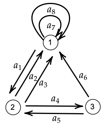
Figure 1: The digraph $\Delta$ in Example 6

Remark 7

Let $\Gamma=(V,E)$ be a finite simple graph and $\Delta=\Delta(\Gamma)$ the symmetric digraph. Note that by definition $\Gamma$ has no loops. Then one can see that $A$ and $B$ are natural generalization of the adjacency matrix $A_{\Gamma}$ and the degree matrix $D_{\Gamma}$ of $\Gamma$ respectively (c.f., [10]). In this case, we have $|{\cal A}_{uv}|=|{\cal A}_{vu}|=1$ for non-empty ${\cal A}(u,v)$. In addition, if we consider the case where $\theta^{\rm G}=\theta^{\rm I}$, i.e., $\tau=\upsilon=1$, then it follows that

$$c_{a}(t)=1-t^{2}$$

for all $a\in{\cal A}$, since $|{\cal A}_{uv}|=1$ if ${\cal A}_{uv}\neq\emptyset$ and the inclusions $\iota_{uv}:{\cal A}_{uv}\rightarrow{\cal A}_{vu}$ are bijective. A simple observation shows that, for $u,v\in V$,

$$a_{uv}=\frac{|{\cal A}_{uv}|}{1-t^{2}},\quad b_{uu}=\frac{|{\cal A}^{(1)}\cap{\cal A}_{u*}|}{1-t^{2}}.$$

One can easily see that $|{\cal A}_{uv}|=1$ iff $\{u,v\}\in E$ (otherwise zero), and $|{\cal A}^{(1)}\cap{\cal A}_{u*}|$ gives the number of edges in $\Gamma$ satisfying $\{u,v\}\in E$ for some $v\in V$. This shows that

$$A_{\Delta}(\theta^{\rm G})=\frac{1}{1-t^{2}}A_{\Gamma},\quad B_{\Delta}(\theta^{\rm G})=\frac{1}{1-t^{2}}D_{\Gamma}.$$

Thus we can regard that the weighted adjacency matrix and the weighted backtrack matrix are, respectively, natural generalization of the adjacency matrix and the degree matrix.

Let $\Delta=(V,{\cal A})$ be a finite digraph. Recall that $M=M_{\Delta}(\theta^{\rm G})=(\theta^{\rm G}(a,a^{\prime}))_{a,a^{\prime}\in{\cal A}}$. Let

$$H=H_{\Delta}(\theta^{\rm G})=(\tau(a^{\prime})\delta_{{\mathfrak{h}}(a){\mathfrak{t}}(a^{\prime})})_{a,a^{\prime}\in{\cal A}},$$

$$J=J_{\Delta}(\theta^{\rm G})=(\upsilon(a^{\prime})\delta_{a^{-1}a^{\prime}})_{a,a^{\prime}\in{\cal A}},$$

$$K=K_{\Delta}(\theta^{\rm G})=(\delta_{{\mathfrak{h}}(a)v})_{a\in{\cal A},v\in V},$$

$$L=L_{\Delta}(\theta^{\rm G})=(\tau(a^{\prime})\delta_{u{\mathfrak{t}}(a^{\prime})})_{u\in V,a^{\prime}\in{\cal A}}.$$

For each arc $a\in{\cal A}$, we consider the following restrictions

$$\begin{array}[]{l}J(a)=(\upsilon(a^{\prime})\delta_{\alpha^{-1}\alpha^{\prime}})_{\alpha,\alpha^{\prime}\in{\cal E}(a)},\\ K(a)=(\delta_{{\mathfrak{h}}(\alpha),v})_{\alpha\in{\cal E}(a),v\in V},\\ L(a)=(\tau(a^{\prime})\delta_{u{\mathfrak{t}}(\alpha^{\prime})})_{u\in V,\alpha^{\prime}\in{\cal E}(a)}\end{array}$$

for the matrices $J$, $K$, and $L$. Note that $J(a)$ is $2\times 2$-matrix if $a\in{\cal A}^{(1)}$, $1\times 1$ otherwise. Hence we can arrange the arcs so as to the matrix $J$ is a direct sum

$$J=\left(\bigoplus_{a\in{\cal A}^{(1)}}J(a)\right)\oplus\left(\bigoplus_{a\in{\cal A}\setminus({\cal A}^{(1)}\cup{\cal A}^{(-1)})}J(a)\right)$$

of $2\times 2$ blocks and $1\times 1$ blocks. We fix such a total order on ${\cal A}$. If we denote by $I(a)$ ($a\in{\cal A}$) the identity matrix of degree $|{\cal E}(a)|$, then the matrix $I+tJ$ is a direct sum of the matrices $\oplus_{a\in{\cal A}\setminus{\cal A}^{(-1)}}(I(a)+tJ(a))$, where the direct summands are all invertible on $R[[t]]$.

Lemma 8

The matrix $I+tJ$ is invertible.

For $\Delta$ and $\theta^{\rm G}$, we denote by $I_{\Delta}(t;\theta^{\rm G})$ the following formal power series with indeterminate $t$:

$$\frac{1}{\det(I+tJ)\det(I-tA_{\Delta}(\theta^{\rm G})+t^{2}B_{\Delta}(\theta^{\rm G}))}.$$

Theorem 9 (Main theorem)

Let $\Delta$, $R$ and $\theta^{\rm G}$ be as above. We have

$$Z_{\Delta}(t;\theta^{\rm G})=I_{\Delta}(t;\theta^{\rm G}).$$

Proof. Recall that we have the identity

$$Z_{\Delta}(t;\theta^{\rm G})=\frac{1}{\det(I-tM)},$$

where $M=M_{\Delta}(\theta^{\rm G})$. Let $H,J,K$ and $L$ be as above. By definition, it follows that $M=H-J$. It also follows that $H=KL$, thus $M=KL-J$. Hence we have

$$\det(I-tM) = \det(I-t(KL-J))$$

$$= \det((I+tJ)-tKL)$$

$$= \det(I+tJ)\det(I-t(I+tJ)^{-1}KL)$$

$$= \det(I+tJ)\det(I-tL(I+tJ)^{-1}K),$$

where the final identity follows from the well-known identity $\det(I-AB)=\det(I-BA)$ in linear algebra. Since each direct summand of

$$I+tJ=\bigoplus_{a\in{\cal A}\setminus{\cal A}^{(-1)}}I(a)+tJ(a)$$

is invertible, we have $(I+tJ)^{-1}=\bigoplus_{a\in{\cal A}\setminus{\cal A}^{(-1)}}(I(a)+tJ(a))^{-1},$ and it follows that

$$L(I+tJ)^{-1}K=\sum_{a\in{\cal A}\setminus{\cal A}^{(-1)}}L(a)(I(a)+tJ(a))^{-1}K(a).$$

Note that $\det(I(a)+tJ(a))=c_{a}(t)$ for $a\in{\cal A}\setminus{\cal A}^{(-1)}$, and we have

$$(I(a)+tJ(a))^{-1}=\left\{\begin{array}[]{ll}c_{a}(t)^{-1}(I(a)-tJ(a)),&\mbox{if $a\in{\cal A}^{(1)}$}\\ c_{a}(t))^{-1}I(a),&\mbox{if $a\in{\cal A}^{(2)}\sqcup{\cal A}^{\times}$}.\end{array}\right.$$

Hence it follows that

$$\sum_{a\in{\cal A}\setminus{\cal A}^{(-1)}}L(a)(I(a)+tJ(a))^{-1}K(a)=\sum_{a\in{\cal A}\setminus{\cal A}^{(-1)}}c_{a}(t)^{-1}L(a)K(a)-t\sum_{a\in{\cal A}^{(1)}}c_{a}(t)^{-1}L(a)J(a)K(a).$$

The $(u,v)$-entry $r_{uv}$ of the matrix $\sum_{a\in{\cal A}\setminus{\cal A}^{(-1)}}c_{a}(t)^{-1}L(a)K(a)$ is given by

$$r_{uv}=\sum_{a\in{\cal A}\setminus{\cal A}^{(-1)}}c_{a}(t)^{-1}\sum_{\alpha\in{\cal E}(a)}\tau(\alpha)\delta_{u{\mathfrak{t}}(\alpha)}\delta_{{\mathfrak{h}}(\alpha)v}.$$ (1)

Note that $\delta_{u{\mathfrak{t}}(\alpha)}\delta_{{\mathfrak{h}}(\alpha)v}\neq 0$ is equivalent to $a\in{\cal A}_{uv}$. It follows that

$$r_{uv}=\sum_{a\in{\cal A}\setminus{\cal A}^{(-1)}}c_{a}(t)^{-1}\sum_{\alpha\in{\cal E}(a)\cap{\cal A}_{uv}}\tau(\alpha).$$

We verify $r_{uv}=a_{uv}$ for all $(u,v)\in V\times V$. Suppose that $u\preceq v$. If $a\in{\cal A}^{{(1)}}$, then ${\cal E}(a)\cap{\cal A}_{uv}=\{a\}$. Otherwise, we have ${\cal E}(a)\cap{\cal A}_{uv}=\emptyset.$ This implies that $r_{uv}=\sum_{a\in{\cal A}\setminus{\cal A}^{(-1)}}c_{a}(t)^{-1}\tau(a).$ In the case where $v\prec u$, ${\cal E}(a)\cap{\cal A}_{uv}\neq\emptyset$ implies that $a\in{\cal A}^{\times}$, and we have ${\cal E}(a)\cap{\cal A}_{uv}=\{a\}$ for $a\in{\cal A}^{\times}$. Suppose that $u=v$. In this case, ${\cal E}(a)\cap{\cal A}_{uu}\neq\emptyset$ implies $a\in{\cal A}^{(2)}$, and we have ${\cal E}(a)\cap{\cal A}_{uu}=\{a\}$. Therefore, putting all these together, it follows that $r_{uv}=a_{uv}$ for all $(u,v)\in V\times V$.

The $(u,v)$-entry $s_{uv}$ of the matrix $\sum_{a\in{\cal A}^{(1)}}c_{a}(t)^{-1}L(a)J(a)K(a)$ is given by

$$s_{uv}=\sum_{a\in{\cal A}^{(1)}}c_{a}(t)^{-1}\sum_{\alpha,\beta\in{\cal E}(a)}\tau(\alpha)\upsilon(\beta)\delta_{u{\mathfrak{t}}(\alpha)}\delta_{\alpha^{-1}\beta}\delta_{{\mathfrak{h}}(\beta)v}.$$ (2)

We verify $s_{uv}=b_{uv}$ for any $(u,v)\in V\times V$. Let $a\in{\cal A}^{(1)}$. We have ${\cal E}(a)=\{a,a^{-1}\}$ with $a\neq a^{-1}$. Thus it follows that

$$s_{uv}=\sum_{a\in{\cal A}^{(1)}}c_{a}(t)^{-1}\tau(a)\upsilon(a^{-1})\delta_{u{\mathfrak{t}}(a)}\delta_{{\mathfrak{h}}(a^{-1})u},$$

which equals $\sum_{a\in{\cal A}^{(1)}\cap{\cal A}_{u*}}c_{a}(t)^{-1}\tau(a)\upsilon(a^{-1}).$ Now we have show that $s_{uv}=b_{uv}$. $\Box$

Acknowledgements

The authors would like to express his deep gratitude to Professor Iwao Sato, Oyama National College of Technology, who suggested the problem considered in this article, for illuminating discussions and valuable comments. The authors also would like to thank anonymous referees for his valuable comments that improve the article. The first named author is partially supported by Grant-in-Aid for JSPS Fellows, Grant Number JP20J20590. The second named author is partially supported by JSPS KAKENHI, Grant Number JP22K03262. The authors also would like to thank anonymous referees for his valuable comments that improve the article.

References

- [1] L. Bartholdi, Counting paths in graphs, Eiseign. Math. 45 (1999), 83-131.
- [2] H. Bass, The Ihara-Selberg zeta function of a tree lattice, Internat. J. Math. 3 (1992), 83-131.
- [3] R. Bowen and O. Lanford, Zeta functions of restrictions of the shift transformation, , Proc. Symp. Pure Math. 14 (1970), 43-50.
- [4] P. Cartier, D. Foata, Problemes combinatoires de commutation et rearrangements, Lecture Notes in Mathematics 85, Springer, Berlin, 1969.
- [5] Y. Choe, J. Kwak, Y. Park and I. Sato, Bartholdi zeta and -functions of weighted digraphs, their covering and products, Adv. Math. 213 (2007), 865-886.
- [6] D. Foata, G.N. Han, Specializations and extensions of the quantum MacMahon Master Theorem, Lin. Alg. Appl. 423 (2007), 445-455.
- [7] D. Foata and D. Zeilberger, A combinatorial proof of Bass’s evaluations of the Ihara-Selberg zeta function for graphs, Trans. Amer. Math. Soc. 355 (1999), 2257-2274.
- [8] K.-i. Hashimoto, On the zeta- and -functions of finite graphs, Internat. J. Math. 1 (1990) 381-396.
- [9] Y. Ihara, On discrete subgroup of the two by two projective linear group over -adic fields, J. Math. Soc. Japan 18 (1966), 219-235.
- [10] Y. Ide, A. Ishikawa, H. Morita, I. Sato and E. Segawa, The Ihara expression for the generalized weighted zeta function of a finite simple graph, Lin. Alg. Appl. 627 (2021), 227-241.
- [11] A. Ishikawa, A family of quantum walks on a finite graph corresponding to the generalized weighted zeta function, https://doi.org/10.48550/arXiv.2211.00904.
- [12] A. Ishikawa and H. Morita, The inverses in digraphs and the Ihara expression, in preparation.
- [13] A. Ishikawa, H. Morita and I. Sato, The Ihara expression for generalized weighted zeta functions of Bartholdi type on finite digraphs, http://arxiv.org/abs/2202.06001.
- [14] N. Konno and I, Sato, On the relation between quantum walks and zeta functions, Quantum Inf. Process. 11 (2012), 341-349.
- [15] M. Konvalinka, I. Pak, Non-commutative extensions of the MacMahon Master Theorem, Adv. Math. 216 (2007), 29-61.
- [16] M. Kotani and T. Sunada, Zeta functions of finite graphs, J. Math. Sci. U. Tokyo 7 (2000), 7-25.
- [17] H. Mizuno and I. Sato, Weighted zeta functions of graphs, J. Combin. Theory Ser. B 91 (2004), 169-183.
- [18] H. Morita, Ruelle zeta functions for finite digraphs, Lin. Alg. Appl. 603 (2020), 329-358.
- [19] S. Northshield, Two proofs of Ihara’s theorem, Emerging applications of number theory (Mineapolis, MN, 1996), 469-478, IMA Vol. Math. Appl., 109, Springer, New York, 1999.
- [20] I. Sato, A new Bartholdi zeta function of a graph, Int. J. Algebra 1 (2007), 269-281.
- [21] J. -P. Serre, Trees, Springer-Verlag, New York, 1980.
- [22] H. Stark and A. Terras, Zeta functions of finite graphs and coverings, Adv. Math. 121 (1996), 124-165.
- [23] T. Sunada, -functions in Geometry and some Applications, in Lecture Note in Math. 1201, pp. 266-284, Springer-Verlag, New York, 1988.
- [24] Y. Watanabe and K. Fukumizu, Graph zeta function in the Bethe free energy and loopy belief propagation, Adv. Neur. Inf. Proc. Sys. 22 (2010), 2017-2025.