Effective potential and superfluidity of microwave-dressed polar molecules

Abstract

For microwave-dressed polar molecules, we analytically derive an intermolecular potential composed of an anisotropic van der Waals shielding core and a long-range dipolar interaction. We validate this effective potential by comparing its scattering properties with those calculated using the full multi-channel interaction potential. It is shown that scattering resonances can be induced by a sufficiently strong microwave field. We also show the power of the effective potential in the study of many-body physics by calculating the critical temperature of the Bardeen-Cooper-Schrieffer pairing in the microwave-dressed NaK gas. It turns out that the effective potential is well-behaved and extremely suitable for studying the many-body physics of the molecular gases. Our results pave the way for the studies of the many-body physics of the ultracold microwave-dressed molecular gases.

Introduction.—Ultracold gases of polar molecules Carr2009 ; Ye2017 provide a unique platform for the exploration of quantum information Zoller2006a , quantum computing DeMille2002 ; Cornish2020 , quantum simulation Zoller2006 ; Zwierlein2021 , quantum chemistry Krem2008 ; Ni2019 , and precision measurement Kozlov2007 ; Berger2010 ; Hinds2011 . From the condensed-matter perspective, the strong long-range and anisotropic dipole-dipole interaction (DDI) make ultracold polar molecules an ideal platform for investigating strongly correlated many-body physics Pfau2009 ; Baranov2012 . Over the past decade, there are tremendous experimental efforts for the creation of the ultracold molecular gases by both direct cooling Tarbutt2021 and cold-atom assembly. Particularly, indirect production of the high-phase-space-density molecular gases from ultracold atomic gases via the Feshbach resonance and stimulated Raman adiabatic passage has been successfully employed to create bialkali molecules of KRb Ye2008 , RbCs Nagerl2014 ; Cornish2014 , NaK Zwierlein2015 ; Bloch2018 ; Ospelkaus2020 , NaRb Wang2016 , NaLi Jamison2017 , and NaCs Will2022 ; Ni2021 . Recently, starting from the association of double degenerate Bose-Fermi mixtures Ye2019 ; Luo2021 and evaporative cooling Ye2020a ; Ye2021 ; Luo2022a enabled by the collisional shielding with either a d.c. Ye2020a ; Ye2021 ; Ye2020b or a microwave field Luo2022a ; Doyle2021 , degenerate Fermi gases of polar molecules have finally become available in experiments.

Unlike the conventional DDI induced by a d.c. electric field, the long-range DDI between microwave-shielded molecules in the highest dressed state is attractive in the plane of the microwave field Luo2022a , which may lead to exotic $p$-wave superfluids You1999 ; Baranov2002 ; Shlyapnikov2009 ; Shi2010 ; Shlyapnikov2011 . Because DDI couples different rotational states, a complete description of the intermolecular interaction involves multiple dressed rotational states of the molecules Karman2018 ; Karman2022 , which is cumbersome for the studies of the many-body physics of a single shielded dressed state. Therefore, a simple and accurate effective potential is an essential ingredient for exploring the many-body physics of molecular gases.

In this Letter, we analytically derive an effective potential between two microwave-dressed polar molecules. At large inter-molecular distance, this potential is a negated DDI such that it is attractive in the plane of the microwave field and repulsive along the propagation direction of microwave. While at short range, the potential is of the $1/r^{6}$ type and is anisotropically repulsive. As a result, the effective potential has a shielding core in all three dimensions. The validity of this effective potential is justified by comparing it with numerically obtained adiabatic potential and by exploring the scattering properties of two molecules. We show that the effective potential not only leads to the correct scattering cross sections, but also accurately predicts the position of the scattering resonance. Finally, as an application of the effective potential, we study the Bardeen-Cooper-Schrieffer (BCS) superfluidity in the microwave-dressed NaK gas, where the Rabi-frequency of the microwave field plays the role as a control knob to tune the superfluid critical temperature. It turns out that the effective potential is well-behaved and suitable for studying the many-body physics of molecular gases.

Effective molecule-molecule interaction.—We consider a gas of the NaK molecules in the ${}^{1}\Sigma(v=0)$ state which exhibits a molecular-frame dipole moment $d=2.72$ Debye. Under ultracold temperature, only the rotational degree of freedom is relevant such that the Hamiltonian of a single molecule is $\hat{h}_{\rm rot}=B_{\rm rot}{\mathbf{J}}^{2}$, where $B_{\rm rot}/\hbar=2\pi\times 2.822\,\mathrm{GHz}$ is the rotational constant and ${\mathbf{J}}$ is the angular momentum operator. Since the rotation spectrum, $B_{\rm rot}J(J+1)$, is anharmonic, we focus on the two lowest rotational manifolds ($J=0$ and $1$) which are split by an energy $\hbar\omega_{e}=2B_{\rm rot}$. Correspondingly, the Hilbert space for the internal states of a molecule is defined by four states: $|J,M_{J}\rangle=|0,0\rangle$, $|1,0\rangle$, and $|1,\pm 1\rangle$. To achieve the microwave shielding, molecules with electric dipole moment $d_{0}\hat{\mathbf{d}}$ are illuminated by a position-independent $\sigma^{+}$-polarized microwave propagating along the z axis, where $\hat{\mathbf{d}}$ is the unit vector along the internuclear axis of the molecule and the microwave field rotates circularly in the $xy$ plane with frequency $\omega_{0}$. Within the internal-state Hilbert space, the coupling between the microwave and the molecular rotational states gives rise to the Hamiltonian $\hat{h}_{\rm mw}=\frac{\hbar\Omega}{2}e^{-i\omega_{0}t}|1,1\rangle\langle 0,0|+{\rm h.c.}$, where $\Omega$ is the Rabi frequency. Then, in the interaction picture, the eigenstates of the internal-state Hamiltonian, $\hat{h}_{\rm in}=\hat{h}_{\rm rot}+\hat{h}_{\rm mw}$, are $|0\rangle\equiv|1,0\rangle$, $|-1\rangle\equiv|1,-1\rangle$, $|+\rangle\equiv u|0,0\rangle+v|1,1\rangle$, and $|-\rangle\equiv u|1,1\rangle-v|0,0\rangle$, where $u=\sqrt{(1-\delta/\Omega_{\mathrm{eff}})/2}$ and $v=\sqrt{(1+\delta/\Omega_{\mathrm{eff}})/2}$ with $\delta=\omega_{e}-\omega_{0}$ being the detuning and $\Omega_{\mathrm{eff}}=\sqrt{\delta^{2}+\Omega^{2}}$ the effective Rabi frequency. The corresponding eigenenergies are $E_{0}=E_{-1}=\delta$ and $E_{\pm}=(\delta\pm\Omega_{\mathrm{eff}})/2$. Figure 1(a) schematically shows the level structure of a molecule.

For two molecules with dipole moments $d\hat{\mathbf{d}}_{1}$ and $d\hat{\mathbf{d}}_{2}$, the dipole-dipole interaction (DDI) between them is

$$V({\mathbf{r}})=\frac{d^{2}}{4\pi\epsilon_{0}r^{3}}\left[\hat{\mathbf{d}}_{1}\cdot\hat{\mathbf{d}}_{2}-3(\hat{\mathbf{d}}_{1}\cdot\hat{\mathbf{r}})(\hat{\mathbf{d}}_{2}\cdot\hat{\mathbf{r}})\right],$$ (1)

where $\epsilon_{0}$ is the electric permittivity of vacuum, $r=|{\mathbf{r}}|$, and $\hat{\mathbf{r}}={\mathbf{r}}/r$. To express DDI in the two-molecule internal Hilbert space, we note that the two-particle Hamiltonian $\hat{H}_{2}=\sum_{j=1,2}\hat{h}_{j}+V({\mathbf{r}}_{1}-{\mathbf{r}}_{2})$ possesses a parity symmetry, where $\hat{h}_{j}=-\hbar^{2}\nabla_{j}^{2}/(2M)+\hat{h}_{\rm in}(j)$ with $M$ being the mass of the molecule. This suggests that the symmetric and antisymmetric two-particle internal states are decoupled in the Hamiltonian $\hat{H}_{2}$. Here we focus on the ten-dimensional symmetric subspace in which the shielding states of the molecules lie. It turns out that, under the rotating-wave approximation, $V({\mathbf{r}})$ in the seven-dimensional (7D) symmetric subspace, $\mathcal{S}_{7}\equiv\{|\nu\rangle\}_{\nu=1}^{7}$, is decoupled from the remaining three-dimensional symmetric subspace, where $|1\rangle=|+,+\rangle$, $|2\rangle=|+,0\rangle_{s}$, $|3\rangle=|+,-1\rangle_{s}$, $|4\rangle=|+,-\rangle_{s}$, $|5\rangle=|-,0\rangle_{s}$, $|6\rangle=|-,-1\rangle_{s}$, and $|7\rangle=|-,-\rangle$ with $|i,j\rangle_{s}=(|i,j\rangle+|j,i\rangle)/\sqrt{2}$. Correspondingly, with respect to the asymptotical state $|\nu=1\rangle$, the energies of these states are $\mathcal{E}_{\nu}=\{0,\frac{1}{2}(\delta-\Omega_{\rm eff}),\frac{1}{2}(\delta-\Omega_{\rm eff}),-\Omega_{\rm eff},\frac{1}{2}(\delta-3\Omega_{\rm eff}),\frac{1}{2}(\delta-3\Omega_{\rm eff}),-2\Omega_{\rm eff}\}$. In below, we shall consider the two-molecule problem only in the subspace $\mathcal{S}_{7}$.

To derive an effective potential between two molecules, we make use of the Born-Oppenheimer approximation which holds when the kinetic energy of the molecules is much smaller than the energy level spacings between internal states ($\sim\Omega_{\mathrm{eff}}$). After diagonalizing $V(\mathbf{r})$ in $\mathcal{S}_{7}$, we find seven adiabatic potentials corresponding to different dressed-state channels [see, e.g., Fig. 1(b) for the typical adiabatic potential curves]. Particularly, the effective potential for two molecules in the dressed state $|+\rangle$ is the highest adiabatic curve. Remarkably, as shown in the Supplemental Material (SM), there exists an approximate expression for the effective potential, i.e.,

$$V_{\mathrm{eff}}(\mathbf{r}) =\frac{C_{3}}{r^{3}}P_{2}(\cos\theta)+\frac{C_{6}}{r^{6}}A(\theta),$$ (2)

where $P_{l}(\cos\theta)$ is the Legendre polynomial with $\theta$ being the polar angle of ${\mathbf{r}}$ and $A(\theta)=7-5P_{2}(\cos\theta)-2P_{4}(\cos\theta)$. Moreover, $C_{3}=d^{2}/\left[24\pi\epsilon_{0}(1+\delta_{r}^{2})\right]$, $C_{6}=d^{4}/\left[1120\pi^{2}\epsilon_{0}^{2}\Omega(1+\delta_{r}^{2})^{3/2}\right]$ with $\delta_{r}=\delta/\Omega$. The first term of $V_{\mathrm{eff}}$ represents DDI which, different from the conventional one, is attractive in the $xy$ plane and repulsive along the $z$ axis. Because $A(\theta)>0$ when $\theta\neq 0$ or $\pi$, the second term is repulsive and provides a shielding core away from the $z$ axis. Interestingly, even along the $z$ axis on which $A(\theta)$ vanishes, DDI itself is repulsive and prevents two molecules from getting close to each other.

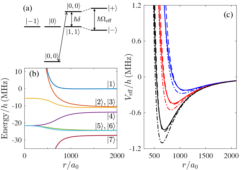
Figure 1: (a) Schematic of the level structure of a microwave-dressed molecule. (b) Typical adiabatic potential curves of two colliding molecules for seven dressed state channels. (c) Effective potentials along $\theta=\pi/2$ obtained by numerical diagonalization (solid lines), numerical fitting (dashed line), and analytical expressions (dash-dotted lines) for $\delta_{r}=0.1$ and $\Omega/(2\pi)=20$, $50$, and $80\,{\rm MHz}$ (for three sets of curves in descending order).

In Fig. 1(c), the effective potential (2) is benchmarked by the highest adiabatic curve obtained from diagonalizing $V(\mathbf{r})$. Generally speaking, the expression for $C_{3}$ is accurate in the sense that it gives rise to the correct long-range behavior, while the analytical expression for $C_{6}$ is a good approximation only when $\Omega>d_{0}^{2}/(4\pi\epsilon_{0}r^{3})$. In any case, one can alternatively determine the values of $C_{3}$ and $C_{6}$ by fitting the adiabatic potential curve, which, as shown in Fig. 1(c) and also in SM, yields satisfactory results in the energy range of interest to us. The advantage of Eq. (2) is that it establishes an intuitive connection between the potential and the physical parameters of the microwave field. In addition, as shall be shown below, this effective potential is well-behaved and can be used for studying the many-body problems.

Two-body scatterings.—To further justify the effective potential, we investigate the low-energy scattering of two shielding molecules interacting via $V_{\rm eff}({\mathbf{r}})$. Since this study only involves a single scattering channel ($\nu=1$ in $\mathcal{S}_{7}$), its results should be checked by the scattering calculations involving all seven channels. To this end, let us briefly outline the theoretical treatment for the multi-channel scattering Karman2018 ; Karman2022 ; Bohn2003 ; Quemener2018 . The Schrödinger equations governing the relative motion of two colliding molecules are

$$\sum_{\nu^{\prime}=1}^{7}\left(-\frac{\hbar^{2}\nabla^{2}}{M}\delta_{\nu\nu^{\prime}}+V_{\nu\nu^{\prime}}\right)\psi_{\nu^{\prime}}({\mathbf{r}})=\frac{\hbar^{2}k_{\nu}^{2}}{M}\psi_{\nu}({\mathbf{r}}),$$ (3)

where $\psi_{\nu}({\mathbf{r}})$ is the wave function of the $\nu$th scattering channel, $V_{\nu\nu^{\prime}}=\langle\nu|V|\nu^{\prime}\rangle$, and $k_{\nu}=\sqrt{k_{1}^{2}-M\mathcal{E}_{\nu}/\hbar^{2}}$ is the incident momentum of the $\nu$th scattering channel. To solve Eq. (3), we first expand the wave functions in the partial-wave basis as $\psi_{\nu}({\mathbf{r}})=\sum_{lm}Y_{lm}(\hat{\mathbf{r}})\phi_{\nu lm}(r)/r$, where $l$ is odd for identical fermions. The equations for $\phi_{\nu lm}$ can be numerically evolved from $r=0$ to a sufficiently large value $r_{\infty}$ using Johnson’s log-derivative propagator method log-Johnson . Then, by comparing $\phi_{\nu lm}$ with the asymptotical boundary condition, we obtain the scattering amplitude $f^{\nu^{\prime}l^{\prime}m^{\prime}}_{\nu lm}$ and cross section $\sigma^{\nu^{\prime}l^{\prime}m^{\prime}}_{\nu lm}=4\pi\left|f^{\nu^{\prime}l^{\prime}m^{\prime}}_{\nu lm}\right|^{2}$ for the $(\nu lm)$ to $(\nu^{\prime}l^{\prime}m^{\prime})$ scattering. It should be noted that $\sigma^{\nu^{\prime}l^{\prime}m^{\prime}}_{\nu lm}$ is nonzero only when $m$ and $m^{\prime}$ satisfy $m=m_{\nu}$ and $m^{\prime}=m_{\nu^{\prime}}$ where, for $\nu=1$ to $7$, $m_{\nu}=m_{1},m_{1}+1,m_{1}+2,m_{1},m_{1}+1,m_{1}+2$, and $m_{1}$, respectively, with $m_{1}$ being an integer. Numerically, to ensure the convergence of the scattering cross sections, we normally choose $k_{0}r_{\infty}>32$ and $l_{c}>11$, where $l_{c}$ is the truncation imposed on the orbital angular momentum.

As a special case of the multi-channel scattering, the Schrödinger equation for single-channel scattering can be obtained by projecting Eq. (3) onto the $\nu=1$ channel with $V_{11}$ being replaced by $V_{\rm eff}$. In addition, we denote the single-channel scattering cross section as $\sigma_{lm}^{l^{\prime}m^{\prime}}$.

Since the scattering cross section of the $p$ wave is dominant over all other partial waves SM , we compare, in Fig. 2(a), $\sigma_{11}^{11}$ and $\sigma_{111}^{111}$ for $\delta_{r}=0.1$ and $k_{1}/k_{F}=0.04$, $0.45$, and $1$, where $k_{F}=(6\pi^{2}n_{0})^{1/3}$ is the Fermi wave vector with $n_{0}=10^{12}\,{\rm cm}^{-3}$ being the density of the experimentally realized molecular gas Luo2022a . As can be seen, away from scattering resonances, quantitative agreements have been achieved for $p$-wave cross section under different incident momenta. Moreover, the single-channel calculations can even predict the position of scattering resonance with high accuracy. These results together with other comparisons in SM validate the usage of the effective potential, which, as shown below, significantly simplifies the calculations in the many-body problems.

As to the $\Omega$ dependence of the $p$-wave cross section, it can be seen that, for small $k_{1}$, $\sigma_{111}^{111}$ barely changes as $\Omega$ varies over a wide range. Then at $\Omega/(2\pi)\approx 87.7\,{\rm MHz}$ a narrow scattering resonance appears, signaling the formation of a quasi-bound state. Furthermore, as $k_{1}$ increases to $k_{F}$, the resonance peak shifts to $\Omega/(2\pi)\approx 73.6\,{\rm MHz}$ and the width of the resonance is significantly broadened. To understand these features, let us recall that 1) there is a centrifugal barrier for the $p$-wave potential; 2) a scattering resonance implies that a quasi-bound state with energy in resonance with the incident energy forms inside the barrier. Now, as $k_{1}$ increases, the resonant quasi-bound state energy also increases and gets closer to the top of the potential barrier. Consequently, the lifetime of the quasi-bound state is shortened due to large decay rate, which leads to a broader resonance. In addition, the increasing quasi-bound state energy implies a weakened attractive interaction via reducing $\Omega$ (see the relation between $C_{6}$ and $\Omega$). Therefore, the resonance peak shifts towards the lower $\Omega$ direction as $k_{1}$ increases.

To reveal more details about the scattering resonance, we map out, in Fig. 2(b), $\sigma_{111}^{111}$ on the $\Omega$-$\delta_{r}$ parameter plane for $k_{1}=0.45k_{F}$. As can be seen, a resonant peak appears in the parameter region $\delta_{r}\apprle 0.3$ and $\Omega/(2\pi)\apprge 80\,{\rm MHz}$. To give an intuitive explanation to the relation between the resonance and control parameters, a $p$-wave bound state at threshold appears when the WKB phase

$$\varphi_{p}=\int_{v_{p}(r)\leq 0}\sqrt{-Mv_{p}(r)/\hbar^{2}}dr\propto\left[\frac{\Omega^{2}}{(1+\delta_{r}^{2})^{5}}\right]^{1/12}$$ (4)

is sufficiently large, where $v_{p}(r)=\int d\hat{\mathbf{r}}|Y_{1m}(\hat{\mathbf{r}})|^{2}V_{\rm eff}({\mathbf{r}})$. Clearly, both increasing $\Omega$ and decreasing $\delta_{r}$ favor the appearance of a shape resonance and the formation of a bound state.

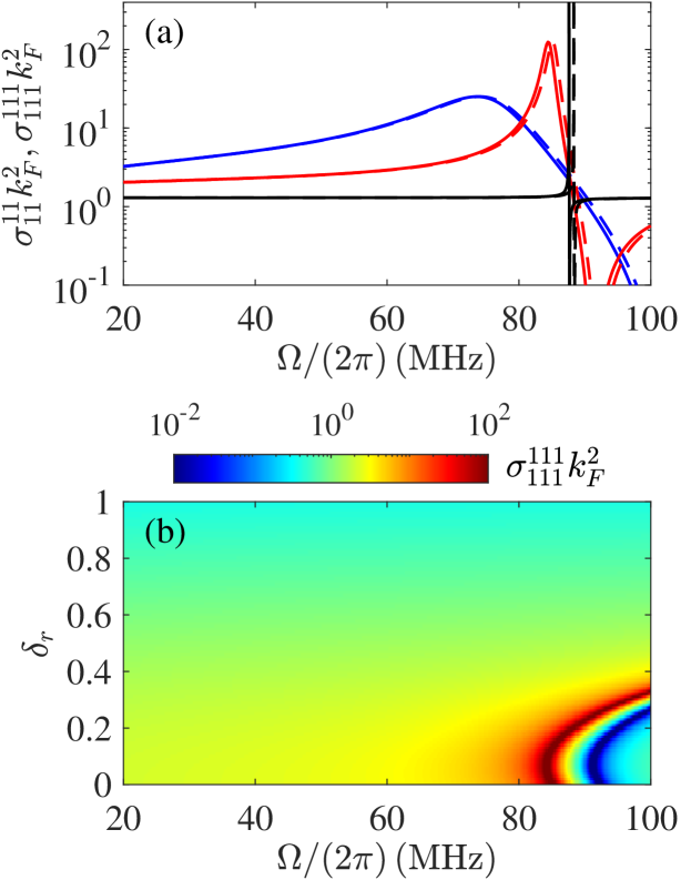
Figure 2: (a) $p$-wave scattering cross sections $\sigma_{11}^{11}k_{F}^{2}$ (solid lines) and $\sigma_{111}^{111}k_{F}^{2}$ (dashed lines) as functions of $\Omega$ for $\delta_{r}=0.1$ and $k_{1}/k_{F}=0.04$ (black lines), $0.45$ (red lines), and $1$ (blue lines). (b) $\sigma_{111}^{111}k_{F}^{2}$ as a function of $\Omega$ and $\delta_{r}$ for $k_{1}/k_{F}=0.45$.

Superfluid phase transitions.—As an application of the effective potential, we now turn to explore the BCS superfluid phase transition in a homogeneous gas of the dressed-state molecules with density $n_{0}$. In particular, we focus on the transition temperature $T_{c}$ and the pairing wave functions. Previously, the superfluidity of the fermionic dipolar gases have been extensively studied using the pseudopotential containing a contact part and a bare DDI You1999 ; Baranov2002 ; Shlyapnikov2009 ; Baranov2004 ; Shlyapnikov2011 ; Marenko2006 ; Shi2010 ; Hirsch2010 ; Pu2010 ; Shi2014 ; Zhai2013 . To illustrate the effect of microwave field to the superfluidity, we apply the effective potential to the molecules in the dressed state $|+\rangle$, and write down the many-body Hamiltonian

$$\hat{H} =\int d^{3}\mathbf{r}\hat{\psi}^{\dagger}(\mathbf{r})\left(-\frac{\hbar^{2}\nabla^{2}}{2M}-\mu\right)\hat{\psi}(\mathbf{r})$$

$$\quad+\frac{1}{2}\int d\mathbf{r}d\mathbf{r}^{\prime}\hat{\psi}^{\dagger}(\mathbf{r})\hat{\psi}^{\dagger}(\mathbf{r}^{\prime})V_{\mathrm{eff}}(\mathbf{r}-\mathbf{r}^{\prime})\hat{\psi}(\mathbf{r}^{\prime})\hat{\psi}(\mathbf{r}),$$ (5)

where $\hat{\psi}({\mathbf{r}})$ is the field operator of the molecules in the dressed state $\left|+\right\rangle$ and $\mu$ is the chemical potential.

In the superconducting phase, the order parameter in the momentum space takes the form

$$\Delta(\mathbf{k})=\int\frac{d{\mathbf{p}}}{(2\pi)^{3}}\widetilde{V}_{\mathrm{eff}}(\mathbf{k}-\mathbf{p})\left\langle c_{-\mathbf{p}}c_{\mathbf{p}}\right\rangle,$$ (6)

where $\widetilde{V}_{\rm eff}({\mathbf{k}})$ is the Fourier transform of $V_{\rm eff}({\mathbf{r}})$, $\hat{c}_{\mathbf{p}}=\int d{\mathbf{r}}\hat{\psi}(\mathbf{r})e^{-i\mathbf{p}\cdot{\mathbf{r}}}/(2\pi)^{3/2}$, and $\left\langle\hat{c}_{-\mathbf{p}}\hat{c}_{\mathbf{p}}\right\rangle$ is the pairing function which, within the mean-field theory, reads $\left\langle\hat{c}_{-\mathbf{p}}\hat{c}_{\mathbf{p}}\right\rangle=-\Delta(\mathbf{p})\tanh(\beta E_{\mathbf{p}}/2)/(2E_{\mathbf{p}})$. Here, $\beta=1/(k_{B}T)$ is the inverse temperature and $E_{\mathbf{p}}=\sqrt{\varepsilon_{\mathbf{p}}^{2}+\left|\Delta(\mathbf{p})\right|^{2}}$ is the dispersion relation of the Bogoliubov quasiparticle with $\varepsilon_{\mathbf{p}}=p^{2}/(2M)-\mu$. As a result, the gap equation becomes Baranov2002

$$\Delta(\mathbf{k})=-\int\frac{d{\mathbf{p}}}{(2\pi)^{3}}\widetilde{V}_{\mathrm{eff}}(\mathbf{k}-\mathbf{p})\frac{\tanh(\beta E_{\mathbf{p}}/2)}{2E_{\mathbf{p}}}\Delta(\mathbf{p}).$$ (7)

We point out that, unlike an ill-defined potential (e.g., the contact interaction and the pure dipolar interaction) which has to be renormalized Baranov2002 ; Baranov2004 ; sademelo1993 to ensure the convergence of the integral in Eq. (7), the effective potential $V_{\rm eff}$ is well-defined due to its repulsive core. As a result, the two-body wave function behaves as $e^{-B/r^{3}}$ ($B>0$) inside the shielding core, which guarantees that Eq. (7) is solvable without the interaction renormalization.

To find the critical temperature, we note that when $T$ approaches $T_{c}$ from below $|\Delta({\mathbf{p}})|\approx 0$ and, subsequently, $E_{\mathbf{p}}\approx\varepsilon_{\mathbf{p}}$. We then expand the gap and interaction in the partial-wave basis as $\Delta(\mathbf{k})=\sum_{lm}Y_{lm}(\hat{k})\Delta_{lm}(k)$ and $\widetilde{V}_{\mathrm{eff}}(\mathbf{k}-\mathbf{p})=(4\pi)^{2}\sum_{ll^{\prime},m}i^{l^{\prime}-l}Y_{lm}(\hat{k})Y_{l^{\prime}m}^{\ast}(\hat{p})\widetilde{V}_{ll^{\prime},m}(k,p)$, respectively, where $l$ and $l^{\prime}$ are odd for identical fermions. Now, Eq. (7) can be rewritten as

$$\Delta_{lm}(k) =-\frac{2}{\pi}\sum_{l^{\prime}}i^{l^{\prime}-l}\int_{0}^{\infty}p^{2}dp\widetilde{V}_{ll^{\prime},m}(k,p)$$

$$\quad\times\frac{\tanh(\beta_{c}\varepsilon_{\mathbf{p}}/2)}{2\varepsilon_{\mathbf{p}}}\Delta_{l^{\prime}m}(p),$$ (8)

where $\beta_{c}=(k_{B}T_{c})^{-1}$. Due to the axial symmetry of the system, $\Delta_{lm}$ for different $m$’s are decoupled in Eq. (8). To proceed further, we focus on the weak interaction regime which allows us to approximate the chemical potential by the Fermi energy, i.e., $\mu\approx\varepsilon_{F}=\hbar^{2}k_{F}^{2}/(2M)$. Equation (8) then becomes an eigenvalue equation of the integral operator for which negative eigenvalues appears only when $T<T_{c}$. This condition allows us to find the critical temperature.

Before presenting the results, it is worthwhile to have a brief discussion on the numerical treatment of Eq. (8). For $l=l^{\prime}=1$, $\widetilde{V}_{ll^{\prime},m}$ contains a divergent term contributed by the $1/r^{6}$ shielding potential through the integral $\int_{0}^{\infty}drj_{l}(kr)j_{l^{\prime}}(pr)/r^{4}$ SM , where $j_{l}$ is the spherical Bessel function. This imposes a difficulty for numerically solving Eq. (8). To remove this divergence, we introduce a truncation $r_{\rm UV}$ on the lower limit of the integration. Consequently, the divergent term is now proportional to $kp/r_{\rm UV}$. Numerically, it is found that the solution of the Eq. (8) converges as $r_{\rm UV}$ is much smaller than the size of the shielding core and all results presented below are obtained with the truncation $k_{F}r_{\rm UV}\leq 10^{-8}$. This divergence can be understood by considering a two-body problem in the momentum space with interaction potential $\widetilde{V}_{\rm eff}$. Without this divergent term, a false bound state localized inside the shielding core would appear, while the divergent term eliminates the existence of any bound states inside the core. Therefore, the false bound state is removed when $r_{\rm UV}$ is much smaller than the size of the shielding core. This momentum regularization scheme can also be applied to interaction potentials of the form $1/r^{n}$, including the van der Waals and the Lennard-Jones potentials. As to the truncation on angular momentum quantum number, we find that $l_{c}=9$ is sufficient to ensure the convergence of the solution. It is numerically found that the highest critical temperature is reached when $m=\pm 1$. Without loss of generality, we always take $m=1$ for all results presented below.

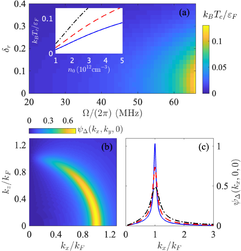
Figure 3: (a) Critical temperature as a function of $\Omega$ and $\delta_{r}$. The inset shows the $n_{0}$ dependence of $T_{c}$ for $\delta_{r}=0.1$ and $\Omega/(2\pi)=28$ (solid line), $38$ (dashed line), and $48\,\mathrm{MHz}$ (dash-dotted line). (b) Momentum distribution of the normalized pairing function $\psi_{\Delta}(k_{x},0,k_{z})$ for $\delta=0.1$ and $\Omega/(2\pi)=58\,\mathrm{MHz}$. (c) The normalized pairing function $\psi_{\Delta}(k_{x},0,0)$ along the $k_{x}$ direction for $\delta_{r}=0.1$ and $\Omega/(2\pi)=48$ (solid line), $58$ (dashed line), and $66\,{\rm MHz}$ (dash-dotted line). Unless otherwise stated, the density of the gas is $n_{0}=10^{12}\,\mathrm{cm}^{-3}$ in this Figure.

In Fig. 3(a), we map out the critical temperature on the $\Omega$-$\delta_{r}$ plane below the BEC transition temperature $T_{c}/\varepsilon_{F}\approx 0.137$ in the strong coupling side sademelo2006 . Here the control parameters are chosen to avoid the scattering resonances where the weak-interaction assumption is violated. As can be seen, $T_{c}$ can be increased by either increasing $\Omega$ or decreasing $\delta_{r}$. This can be roughly understood using Eq. (4) as both increasing $\Omega$ and decreasing $\delta_{r}$ can enhance the attractive interaction. Moreover, the observation that the critical temperature can be efficiently increased by varying $\Omega$ for a fixed effective dipolar strength $C_{3}$ suggests that the critical temperature is mainly determined by the scattering properties at $k_{1}\approx k_{F}$ as Cooper pairs of molecules form at the vicinity of the Fermi surface. In fact, unlike the cross section of the threshold scatterings ($k_{1}\rightarrow 0$) which barely changes for $\Omega/(2\pi)$ up to $80\,{\rm MHz}$ [see Fig. 2(b)], the scattering cross section at $k_{1}\approx k_{F}$ is sensitive to the variation of $\Omega$. The inset of Fig. 3(a) plots $T_{c}$ as a function of the gas density $n_{0}$ for $\delta_{r}=0.1$ and various $\Omega$’s. Apparently, the critical temperature can be dramatically increased with the growing gas density. In particular, for a typical Rabi frequency $\Omega/(2\pi)=38\,\mathrm{MHz}$, $T_{c}$ can be increased by roughly one order of magnitude when $n_{0}$ increases from $10^{12}$ to $5\times 10^{12}\,\mathrm{cm}^{-3}$.

In Fig. 3(b), we present the momentum distribution of the normalized pairing function $\psi_{\Delta}(\mathbf{k})\equiv\left\langle c_{\mathbf{k}}c_{-\mathbf{k}}\right\rangle$ on the $k_{x}$-$k_{z}$ plane. As can be seen, the pairing function $\psi_{\Delta}(\mathbf{k})$ displays a peak at the Fermi momentum $k_{F}$, suggesting that Cooper pairs are formed around the Fermi surface in the BCS regime. Moreover, $\psi_{\Delta}(\mathbf{k})$ exhibits a clear anisotropy on the $k_{x}$-$k_{z}$ plane and is dominated by the $p$ wave as $\int k^{2}dk\,|\!\int d\hat{\mathbf{k}}\psi_{\Delta}({\mathbf{k}})Y_{10}(\hat{\mathbf{k}})|^{2}\apprge 0.97$ for all paring functions obtained in this work. Due to the distinct scattering behavior of microwave shielded molecules, this $p$-wave superfluid Baranov2002 ; Baranov2004 ; Marenko2006 ; sademelo2006 ; Jin2008 is achieved over a broad range of Rabi frequency. Finally, we plot, in Fig. 3(c), $\psi_{\Delta}(\mathbf{k})$ along the $k_{x}$ direction for $n_{0}=10^{12}\,{\rm cm}^{-3}$, $\delta_{r}=0.1$, and various $\Omega$’s. As can be seen, the width of the peak increases with increasing $\Omega$, indicating that, under a stronger attractive interaction, Cooper pairs are formed over a broader range of momentum.

Conclusion and discussion.—We have analytically derived an effective intermolecular potential for microwave-dressed polar molecules. The validity of the effective potential has been justified by studying the low-energy scatterings of two molecules. It has been shown that the results from single-channel scattering calculations using the effective potential are in good agreement with multi-channel results calculated using the realistic potential. We have also explored the many-body physics of the microwave-dressed NaK gas by calculating the critical temperature of the $p$-wave superfluid and the pairing wave function, which proves that the effective potential is well-behaved and suitable for studying the many-body physics of the molecular gases.

Consider the rich many-body physics across a Feshbach resonance sademelo1993 ; sademelo2006 , it is not surprising to expect similar situation from an ultracold gas of polar molecules in resonant regime. However, as shown in this work, a major challenge for experimental realization of dipolar resonances is the requirement for a large Rabi frequency $\Omega$ that is beyond the reach of the current experiments. It turns out that this can potentially be circumvented by employing an elliptically polarized microwave field Luo2022b ; SM . For typical experimental setups, even a small mixing angle can dramatically reduce the resonance Rabi frequency to a value reachable in current experiments.

T.S. thanks Peng Zhang for the stimulating discussion. This work was supported by National Key Research and Development Program of China (Grant No. 2021YFA0718304), by the NSFC (Grants No. 12135018, No. 11974363, No. 12047503, and No. 12274331), and by the Strategic Priority Research Program of CAS (Grant No. XDB28000000). X.-Y. C. and X.-Y. L. acknowledge support from the Max Planck Society, the European Union (PASQuanS Grant No. 817482) and the Deutsche Forschungsgemeinschaft under German Excellence Strategy – EXC-2111 – 390814868 and under Grant No. FOR 2247.

Supplemental Materials

This Supplemental Material is structured as follows. In Section S1, we derive the effective potential $V_{\mathrm{eff}}$ for two molecules in the highest dressed state channel. In Section S2, we first outline formulation for the multichannel scattering calculation and then present additional comparison to justify the effective potential. In Section S3, we derive the partial-wave expansion of the effective potential in the momentum space.

S1 Derivation of the effective potential

To obtain the effective interaction potential between two molecules in the highest dressed-state channel. For convenience, let us first write out the two-particle Hamiltonian

$$\hat{H}_{2}\approx\sum_{j=1,2}\hat{h}_{\rm in}(j)+V({\mathbf{r}}_{1}-{\mathbf{r}}_{2})$$ (S1)

where we have neglected the kinetic energy via the Born-Oppenheimer approximation. Moreover, it is more convenient to express the dipole-dipole interaction as

$$V({\mathbf{r}})=-8\sqrt{\frac{2}{15}}\pi^{3/2}\frac{d^{2}}{4\pi\epsilon_{0}r^{3}}\sum_{m=-2}^{2}Y_{2m}^{\ast}(\hat{\mathbf{r}})\Sigma_{2,m},$$ (S2)

where $Y_{2m}(\hat{\mathbf{r}})$ are spherical harmonics and $\Sigma_{2}$ is an rank-2 spherical tensor with components

$$\Sigma_{2,0}=\frac{1}{\sqrt{6}}(\hat{d}_{1}^{+}\hat{d}_{2}^{-}+\hat{d}_{1}^{-}\hat{d}_{2}^{+}+2\hat{d}_{1}^{0}\hat{d}_{2}^{0}),\;\Sigma_{2,\pm 1}=\frac{1}{\sqrt{2}}(\hat{d}_{1}^{\pm}\hat{d}_{2}^{0}+\hat{d}_{1}^{0}\hat{d}_{2}^{\pm}),\;\mbox{and }\Sigma_{2,\pm 2}=\hat{d}_{1}^{\pm}\hat{d}_{2}^{\pm}.$$ (S3)

Here $\hat{d}_{j}^{\pm}=Y_{1,\pm 1}(\mathbf{\hat{d}}_{j})$ and $\hat{d}_{j}^{0}=Y_{1,0}(\mathbf{\hat{d}}_{j})$ with $\mathbf{\hat{d}}_{j=1,2}$ being the unit vector along the directions of the $j$th dipole moment. Apparently, we have $\hat{d}_{j}^{-}=-(\hat{d}_{j}^{+})^{\dagger}$.

In principle, to obtain an effective potential, one should diagonalize $\hat{H}_{2}$ in the two-particle Hilbert space $\mathcal{H}_{1}\otimes\mathcal{H}_{1}$, where $\mathcal{H}_{1}={\rm span}\{|0,0\rangle,|1,1\rangle,|1,0\rangle,|1,-1\rangle\}$ is the Hilbert space for the internal states of a molecule. To this end, we first note that, in the frame co-rotating with the microwave, the operators $\hat{d}^{\pm,0}$ can be expressed as

$$\hat{d}^{0}=\frac{1}{\sqrt{4\pi}}(\left|1,0\right\rangle\left\langle 0,0\right|e^{i\omega_{0}t}+\mathrm{H.c.}),\;\hat{d}^{+}=\frac{1}{\sqrt{4\pi}}(\left|1,1\right\rangle\left\langle 0,0\right|e^{i\omega_{0}t}-\left|0,0\right\rangle\left\langle 1,-1\right|e^{-i\omega_{0}t}),\mbox{ and }\hat{d}^{-}=-(\hat{d}^{+})^{\dagger}.$$ (S4)

After substituting Eq. (S4) into (S3), the components of the rank-2 spherical tensor $\Sigma_{2}$ become

$$\Sigma_{2,0} =\frac{1}{4\pi\sqrt{6}}\Big{(}2\left|1,0\right\rangle\left\langle 0,0\right|\otimes\left|0,0\right\rangle\left\langle 1,0\right|-\left|1,1\right\rangle\left\langle 0,0\right|\otimes\left|0,0\right\rangle\left\langle 1,1\right|-\left|0,0\right\rangle\left\langle 1,-1\right|\otimes\left|1,-1\right\rangle\left\langle 0,0\right|+\mathrm{H.c.}\Big{)}$$

$$\Sigma_{2,1} =\frac{1}{4\pi\sqrt{2}}\Big{(}\left|1,1\right\rangle\left\langle 0,0\right|\otimes\left|0,0\right\rangle\left\langle 1,0\right|-\left|0,0\right\rangle\left\langle 1,-1\right|\otimes\left|1,0\right\rangle\left\langle 0,0\right|+\left|0,0\right\rangle\left\langle 1,0\right|\otimes\left|1,1\right\rangle\left\langle 0,0\right|$$

$$\quad-\left|1,0\right\rangle\left\langle 0,0\right|\otimes\left|0,0\right\rangle\left\langle 1,-1\right|\Big{)},$$

$$\Sigma_{2,-1} =-\Sigma_{2,1}^{\dagger},$$

$$\Sigma_{2,2} =-\frac{1}{4\pi}\Big{(}\left|1,1\right\rangle\left\langle 0,0\right|\otimes\left|0,0\right\rangle\left\langle 1,-1\right|+\left|0,0\right\rangle\left\langle 1,-1\right|\otimes\left|1,1\right\rangle\left\langle 0,0\right|\Big{)},$$

$$\Sigma_{2,-2} =\Sigma_{2,2}^{\dagger},$$

where we have adopted the rotating-wave approximation by neglecting the high-frequency oscillation terms.

To diagonalize $\hat{H}_{2}$, it is more convenient to proceed in the dressed-state basis $\{|+\rangle,|0\rangle,|-1\rangle,|-\rangle\}$ in which $\hat{h}_{\rm in}(j)$ is diagonal. Moreover, because $\hat{H}_{2}$ possesses a parity symmetry, its eigenstates must be either symmetric or antisymmetric. The fact that the microwave shielded state lies in the symmetric sector allows us to focus on the ten-dimensional symmetric subspace. Fortunately, it turns out that $V({\mathbf{r}})$ in the seven-dimensional symmetric subspace, $\mathcal{S}_{7}$, is decoupled from the remaining three-dimensional symmetric subspace. Then under the basis $\{|\nu\rangle\}_{\nu=1}^{7}$, we have

$$\hat{h}_{\rm in}(1)+\hat{h}_{\rm in}(2) =\begin{pmatrix}0&0&0&0&0&0&0\\ 0&\frac{1}{2}(\delta-\Omega_{\mathrm{eff}})&0&0&0&0&0\\ 0&0&\frac{1}{2}(\delta-\Omega_{\mathrm{eff}})&0&0&0&0\\ 0&0&0&-\Omega_{\mathrm{eff}}&0&0&0\\ 0&0&0&0&\frac{1}{2}(\delta-3\Omega_{\mathrm{eff}})&0&0\\ 0&0&0&0&0&\frac{1}{2}(\delta-3\Omega_{\mathrm{eff}})&0\\ 0&0&0&0&0&0&-2\Omega_{\mathrm{eff}}\\ \end{pmatrix},$$

$$\Sigma_{2,0} =\frac{1}{4\pi\sqrt{6}}\begin{pmatrix}-2u^{2}v^{2}&0&0&-\sqrt{2}uv(u^{2}-v^{2})&0&0&2u^{2}v^{2}\\ 0&2u^{2}&0&0&-2uv&0&0\\ 0&0&-u^{2}&0&0&uv&0\\ -\sqrt{2}uv(u^{2}-v^{2})&0&0&-(u^{2}-v^{2})^{2}&0&0&\sqrt{2}uv(u^{2}-v^{2})\\ 0&-2uv&0&0&2v^{2}&0&0\\ 0&0&uv&0&0&-v^{2}&0\\ 2u^{2}v^{2}&0&0&\sqrt{2}uv(u^{2}-v^{2})&0&0&-2u^{2}v^{2}\end{pmatrix},$$

$$\Sigma_{2,1} =\frac{1}{4\pi\sqrt{2}}\begin{pmatrix}0&\sqrt{2}u^{2}v&0&0&-\sqrt{2}uv^{2}&0&0\\ 0&0&-u^{2}&0&0&uv&0\\ 0&0&0&0&0&0&0\\ 0&u(u^{2}-v^{2})&0&0&-v(u^{2}-v^{2})&0&0\\ 0&0&uv&0&0&-v^{2}&0\\ 0&0&0&0&0&0&0\\ 0&-\sqrt{2}u^{2}v&0&0&\sqrt{2}uv^{2}&0&0\end{pmatrix},$$

$$\Sigma_{2,2} =-\frac{1}{4\pi}\begin{pmatrix}0&0&\sqrt{2}u^{2}v&0&0&-\sqrt{2}uv^{2}&0\\ 0&0&0&0&0&0&0\\ 0&0&0&0&0&0&0\\ 0&0&u(u^{2}-v^{2})&0&0&-v(u^{2}-v^{2})&0\\ 0&0&0&0&0&0&0\\ 0&0&0&0&0&0&0\\ 0&0&-\sqrt{2}u^{2}v&0&0&\sqrt{2}uv^{2}&0\end{pmatrix}.$$

Now, for a given $\mathbf{r}$, we diagonal the $7\times 7$ matrix

$$\hat{H}_{2}=\sum_{j=1,2}\hat{h}_{\rm in}(j)-8\sqrt{\frac{2}{15}}\pi^{3/2}\frac{d^{2}}{4\pi\epsilon_{0}r^{3}}\sum_{m=-2}^{2}Y_{2m}^{\ast}(\hat{\mathbf{r}})\Sigma_{2,m},$$ (S5)

the highest adiabatic curve then corresponds to the effective potential for the microwave-shielded state. Interestingly, it is found that, in the region where the inter-molecular distance is larger than the shielding core, the contributions to the highest eigenstate is dominated by the states $\left|1\right\rangle$, $\left|2\right\rangle$, and $|3\rangle$. Therefore, we may project $\hat{H}_{2}$ onto the three-dimemsional subspace spanned by $\{|1\rangle,|2\rangle,|3\rangle\}$ and obtain the reduced two-body Hamiltonian

$$\hat{H}_{2}^{\prime}(\mathbf{r})=\begin{pmatrix}Du^{2}v^{2}(\cos^{2}\theta-\frac{1}{3})&Du^{2}v\sin\theta\cos\theta e^{-i\varphi}&\frac{1}{\sqrt{2}}Du^{2}v\sin^{2}\theta e^{-2i\varphi}\\ Du^{2}v\sin\theta\cos\theta e^{i\varphi}&\frac{1}{2}(\delta-\Omega_{\mathrm{eff}})-Du^{2}(\cos^{2}\theta-\frac{1}{3})&-\frac{1}{\sqrt{2}}Du^{2}\sin\theta\cos\theta e^{-i\varphi}\\ \frac{1}{\sqrt{2}}Du^{2}v\sin^{2}\theta e^{2i\varphi}&-\frac{1}{\sqrt{2}}Du^{2}\sin\theta\cos\theta e^{i\varphi}&\frac{1}{2}(\delta-\Omega_{\mathrm{eff}})+\frac{1}{2}Du^{2}(\cos^{2}\theta-\frac{1}{3})\end{pmatrix}.$$ (S6)

where $D=d^{2}/(4\pi\epsilon_{0}r^{3})$. We then introduce a unitary transformation

$$U_{2}=\begin{pmatrix}1&0&0\\ 0&\sqrt{\frac{2}{\cos^{2}\theta+1}}\cos\theta&-\frac{1}{\sqrt{\cos^{2}\theta+1}}\sin\theta e^{-i\varphi}\\ 0&\frac{1}{\sqrt{\cos^{2}\theta+1}}\sin\theta e^{i\varphi}&\sqrt{\frac{2}{\cos^{2}\theta+1}}\cos\theta\end{pmatrix}$$ (S7)

which transfers $\hat{H}_{2}^{\prime}$ into

$$\hat{H}_{2}^{\prime\prime}\equiv U_{2}^{\dagger}\hat{H}_{2}^{\prime}U_{2}=\begin{pmatrix}Du^{2}v^{2}(\cos^{2}\theta-\frac{1}{3})&\frac{1}{\sqrt{2}}Du^{2}v\sin\theta\sqrt{\cos^{2}\theta+1}e^{-i\varphi}&0\\ \frac{1}{\sqrt{2}}Du^{2}v\sin\theta\sqrt{\cos^{2}\theta+1}e^{i\varphi}&\frac{1}{2}(\delta-\Omega_{\mathrm{eff}})-\frac{1}{2}Du^{2}(\cos^{2}\theta+\frac{1}{3})&0\\ 0&0&\frac{1}{2}(\delta-\Omega_{\mathrm{eff}})+\frac{1}{3}Du^{2}\end{pmatrix}.$$ (S8)

We can now diagonalize the upper $2\times 2$ matrix and obtain the adiabatic potential curve of the highest dressed-state channel $|1\rangle$,

$$V_{\mathrm{adia}}^{|1\rangle}(\mathbf{r}) =\frac{1}{2}\left[\frac{1}{2}(\delta-\Omega_{\mathrm{eff}})+\frac{1}{3}Du^{2}v^{2}(3\cos^{2}\theta-1)-\frac{1}{6}Du^{2}(3\cos^{2}\theta+1)\right]$$

$$\quad+\sqrt{\frac{1}{4}\left[-\frac{1}{2}(\delta-\Omega_{\mathrm{eff}})+\frac{1}{3}Du^{2}v^{2}(3\cos^{2}\theta-1)+\frac{1}{6}Du^{2}(3\cos^{2}\theta+1)\right]^{2}+\frac{1}{2}D^{2}u^{4}v^{2}\sin^{2}\theta(\cos^{2}\theta+1)}.$$ (S9)

After expanding $V_{\mathrm{adia}}^{|1\rangle}(\mathbf{r})$ to the order $D^{2}$, we obtain the effective interaction potential $V_{\mathrm{eff}}(\mathbf{r})$. It should be noted that the effective potential works very well when the intermolecular distance satisfies $r^{3}>d^{2}/(4\pi\epsilon_{0}\Omega)$. For the validity of the effective potential, we present addition comparisons for $\theta=\pi/3$ and $\pi/4$ in Fig. S1. As can be seen, the effective potentials $V_{\mathrm{eff}}(\mathbf{r})$ and the exact adiabatic potential are in very good agreement.

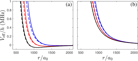
Figure S1: Comparison of the exact adiabatic potential (solid lines) with the fitted effective potential (dashed line) along the angles $\theta=\pi/3$ (a) and $\pi/4$ (b). Other parameters are $\delta_{r}=0.1$ and $\Omega/(2\pi)=20$, $50$, and $80\,\mathrm{MHz}$ (for three sets of curves in descending order).

Finally, in addition to the circular polarized microwave as discussed in the present, the elliptically polarized microwave field of the form $\Omega(\cos\alpha_{m}\sigma^{+}+\sin\alpha_{m}\sigma^{-})$ can also be used to shield the molecules, where $\alpha_{m}$ is the elliptic angle of the left- and right-circularized microwave fields. Then, for small elliptic angle $\alpha_{m}$, one can also derive an analytic expression for the effective potential by following the same procedure, i.e.,

$$V_{\mathrm{eff}}(\alpha_{m},\mathbf{r}) =\frac{C_{3}}{2r^{3}}\left(3\cos^{2}\theta-1+3\sin 2\alpha_{m}\sin^{2}\theta\cos 2\varphi\right)$$

$$\quad+\frac{35C_{6}}{4r^{6}}\sin^{2}\theta\left(\cos^{2}\theta+1-2\sin 2\alpha_{m}\cos^{2}\theta\cos 2\varphi-\sin^{2}2\alpha_{m}\sin^{2}\theta\cos^{2}2\varphi\right).$$ (S10)

S2 Two-body scatterings

Here we outline the procedure for solving the multi-channel scattering problem and present additional comparison between the single- and multi-channel results. To this end, let us first write down the multi-channel Schrödinger equations

$$\sum_{\nu^{\prime}=1}^{7}\left(-\frac{\hbar^{2}\nabla^{2}}{M}\delta_{\nu\nu^{\prime}}+V_{\nu\nu^{\prime}}\right)\psi_{\nu^{\prime}}({\mathbf{r}})=\frac{\hbar^{2}k_{\nu}^{2}}{M}\psi_{\nu}({\mathbf{r}}),$$ (S11)

where $\hbar^{2}k_{\nu}^{2}/M$ is the incident energy of the $\nu$th channel. In general, one should expand $\psi_{\nu}$ in the partial wave basis as $\psi_{\nu}=\sum_{l_{\nu}m_{\nu}}r^{-1}\phi_{\nu l_{\nu}m_{\nu}}Y_{l_{\nu}m_{\nu}}(\hat{\mathbf{r}})$ with $l_{\nu}$ being odd. However, it turns out that, for a given $m$, only these partial wave with $m_{\nu}=m,m+1,m+2,m,m+1,m+2$, and $m$ for $\nu=1$ to $7$ are coupled. Therefore, we may treat each $m$ separately by expanding the scattering wave function as

$$\psi_{\nu=1,4,7}(\mathbf{r}) = \sum_{l}\frac{1}{r}Y_{lm}(\hat{r})\phi_{\nu l}(r),$$

$$\psi_{\nu=2,5}(\mathbf{r}) = \sum_{l}\frac{1}{r}Y_{lm+1}(\hat{r})\phi_{\nu l}(r),$$

$$\psi_{\nu=3,6}(\mathbf{r}) = \sum_{l}\frac{1}{r}Y_{lm+2}(\hat{r})\phi_{\nu l}(r),$$

where we have ignored the quantum number for the projection of the orbital angular momentum. Now, the Schrödinger for the partial waves becomes

$$\sum_{\nu^{\prime}l^{\prime}}\left[-\frac{\hbar^{2}}{M}\left(\frac{\partial^{2}}{\partial r^{2}}-\frac{l(l+1)}{r^{2}}\right)\delta_{\nu\nu^{\prime}}\delta_{ll^{\prime}}-\frac{d_{0}^{2}}{4\pi\epsilon_{0}r^{3}}\sum_{j}(\Xi_{j}^{m})_{\nu l,\nu^{\prime}l^{\prime}}\right]\phi_{\nu^{\prime}l^{\prime}}(r)=\frac{k_{\nu}^{2}}{M}\phi_{\nu l}(r),$$ (S12)

where

$$(\Xi_{0}^{m})_{\nu l,\nu^{\prime}l^{\prime}} = 4\pi\sqrt{\frac{2(2l^{\prime}+1)}{3(2l+1)}}\Sigma_{2,0}C_{l^{\prime}020}^{l0}\,\mathrm{diag}(C_{l^{\prime}m20}^{lm},C_{l^{\prime}m+120}^{lm+1},C_{l^{\prime}m+220}^{lm+2},C_{l^{\prime}m20}^{lm},C_{l^{\prime}m+120}^{lm+1},C_{l^{\prime}m+220}^{lm+2},C_{l^{\prime}m20}^{lm}),$$

$$(\Xi_{1}^{m})_{\nu l,\nu^{\prime}l^{\prime}} = -4\pi\sqrt{\frac{2(2l^{\prime}+1)}{3(2l+1)}}\Sigma_{2,1}C_{l^{\prime}020}^{l0}\,\mathrm{diag}(0,C_{l^{\prime}m+12-1}^{lm},C_{l^{\prime}m+22-1}^{lm+1},0,C_{l^{\prime}m+12-1}^{lm},C_{l^{\prime}m+22-1}^{lm+1},0),$$

$$(\Xi_{2}^{m})_{\nu l,\nu^{\prime}l^{\prime}} = 4\pi\sqrt{\frac{2(2l^{\prime}+1)}{3(2l+1)}}\Sigma_{2,2}C_{l^{\prime}020}^{l0}C_{l^{\prime}m+22-2}^{lm},$$

are the interaction matrix elements with $\mathrm{diag}(\cdots)$ denoting the diagonal matrix and $C_{l^{\prime}m^{\prime}l^{\prime\prime}m^{\prime\prime}}^{lm}\equiv\langle lm|l^{\prime}m^{\prime};l^{\prime\prime}m^{\prime\prime}\rangle$ the short-hand notation for the Clebsch-Gordan coefficients. Apparently, we have $\Xi_{-1}^{m}=\Xi_{1}^{m\dagger}$ and $\Xi_{-2}^{m}=\Xi_{2}^{m\dagger}$.

The coupled channel Schrödinger Eq. (S12) can be solved using the log-derivative method with high precision. In the compact form, Eq. (S12) reads

$$\left[\frac{\partial^{2}}{\partial r^{2}}+\mathcal{V}(r)\right]\phi(r)=0,$$ (S13)

where the potential

$$\mathcal{V}(r)=\left[k_{\nu}^{2}-\frac{l(l+1)}{r^{2}}\right]\delta_{\nu\nu^{\prime}}\delta_{ll^{\prime}}+M\frac{d_{0}^{2}}{4\pi\epsilon_{0}r^{3}}\sum_{j}(\Xi_{j}^{m})_{\nu l,\nu^{\prime}l^{\prime}}.$$ (S14)

Now we define the matrix $\mathbf{\phi}(r)$ whose columns denote the scattering wavefunctions for the incident waves in different channels, i.e., the angular momentum $l$ and dressed-state channels. It follows from Eq. (S13) that the matrix $\mathcal{Y}(r)=\partial_{r}\mathbf{\phi}(r)\mathbf{\phi}^{-1}(r)$ satisfies

$$\partial_{r}\mathcal{Y}(r)=-\mathcal{V}(r)-\mathcal{Y}^{2}(r).$$ (S15)

By solving Eq. (S15) numerically with an appropriate boundary condition $\mathcal{Y}(0)=10^{20}$, we obtain $\mathcal{Y}(r)$ in the asymptotic limit $r\rightarrow\infty$.

On the other hand, for the incident particles with angular momentum $l$ in the dressed-state channel $\nu\in S_{7}$, the asymptotic wavefunction ($r\rightarrow\infty$)

$$\phi_{\nu^{\prime}l^{\prime},\nu l}^{\mathrm{a}}(r)=\mathbf{J}_{l}(k_{\nu}r)\delta_{ll^{\prime}}\delta_{\nu\nu^{\prime}}+\sum_{\nu^{\prime}l^{\prime}}\mathbf{N}_{l^{\prime}}(k_{\nu^{\prime}}r)K_{\nu^{\prime}l^{\prime},\nu l},$$ (S16)

can be obtained analytically, where $\mathbf{J}_{l}(k_{\nu}r)=k_{\nu}^{-1/2}\hat{\jmath}_{l}(k_{\nu}r)$ and $\mathbf{N}_{l}(k_{\nu}r)=k_{\nu}^{-1/2}\hat{n}_{l}(k_{\nu}r)$ are determined by the Riccati-Bessel functions $\hat{\jmath}_{l}(z)=zj_{l}(z)$ and $\hat{n}_{l}(z)=-zn_{l}(z)$, and $K_{\nu^{\prime}l^{\prime},\nu l}$ is the $K$-matrix element for in-coming particles with angular momentum $l$ in the channel $\nu$ and out-going particles with angular momentum $l^{\prime}$ in the channel $\nu^{\prime}$. By matching the numerical solution $\mathcal{Y}(r\rightarrow\infty)$ and $\partial_{r}\mathbf{\phi}^{\mathrm{a}}(r)\mathbf{\phi}^{\mathrm{a}-1}(r)$ determined by Eq. (S16), we can obtain the $K$-matrix element and the scattering amplitude

$$f_{\nu^{\prime}l^{\prime},\nu l}=i\frac{1}{\sqrt{k_{\nu^{\prime}}}}\left(\frac{1}{K+i}K\right)_{\nu^{\prime}l^{\prime},\nu l}\frac{1}{\sqrt{k_{\nu}}}$$ (S17)

from the channel $(\nu l)$ to the channel $(\nu^{\prime}l^{\prime})$, and the partial wave scattering cross section $\sigma_{\nu^{\prime}l^{\prime},\nu l}=4\pi\left|f_{\nu^{\prime}l^{\prime},\nu l}\right|^{2}$. We can also define the average elastic and inelastic scattering cross sections $\sigma_{\nu}^{\mathrm{el}}=\sum_{ll^{\prime}}\sigma_{\nu l^{\prime},\nu l}$ and $\sigma_{\nu}^{\mathrm{inel}}=\sum_{\nu^{\prime},ll^{\prime}}k_{\nu^{\prime}}\sigma_{\nu^{\prime}l^{\prime},\nu l}/k_{\nu}$.

To justify the effective potential, we solve the single channel Schrödinger equation

$$\left[-\frac{\hbar^{2}\nabla^{2}}{M}+V_{\mathrm{eff}}(\mathbf{r})\right]\psi_{++}(\mathbf{r})=\frac{k_{1}^{2}}{M}\psi_{++}(\mathbf{r})$$ (S18)

with the effective potential $V_{\mathrm{eff}}(\mathbf{r})$. In the angular momentum basis $\psi_{++}(\mathbf{r})=\sum_{l}Y_{lm}(\hat{r})\phi_{l}(r)/r$, $\phi_{l}(r)$ satisfies

$$\sum_{l^{\prime}}\left[-\frac{\hbar^{2}}{M}\left(\frac{\partial^{2}}{\partial{r}^{2}}-\frac{l(l+1)}{r^{2}}\right)\delta_{ll^{\prime}}+V_{\mathrm{eff,}ll^{\prime}}^{m}(r)\right]\phi_{l^{\prime}}(r)=\frac{k_{1}^{2}}{M}\phi_{l}(r),$$ (S19)

where the pseudo-potential

$$V_{\mathrm{eff,}ll^{\prime}}^{m}(r)=\frac{C_{3}}{r^{3}}\sqrt{\frac{2l^{\prime}+1}{2l+1}}C_{l^{\prime}020}^{l0}C_{l^{\prime}m20}^{lm}+\frac{C_{6}}{r^{6}}\sqrt{\frac{2l^{\prime}+1}{2l+1}}(7\delta_{ll^{\prime}}-5C_{l^{\prime}020}^{l0}C_{l^{\prime}m20}^{lm}-2C_{l^{\prime}040}^{l0}C_{l^{\prime}m40}^{lm}).$$ (S20)

The Eq. (S19) is solved via the log-derivative method. By defining

$$\mathcal{V}(r)=[k_{1}^{2}-\frac{l(l+1)}{r^{2}}]\delta_{ll^{\prime}}-MV_{\mathrm{eff,}ll^{\prime}}^{m}(r),$$ (S21)

we can rewrite Eq. (S19) as the same form of Eq. (S13) and obtain $\mathcal{Y}(r)$. By matching the numerical solution $\mathcal{Y}(r\rightarrow\infty)$ with the analytical asymptotic wavefunction

$$\phi_{l^{\prime}l}^{\mathrm{a}}(r)=\mathbf{J}_{l}(k_{1}r)\delta_{ll^{\prime}}+\sum_{l^{\prime}}\mathbf{N}_{l^{\prime}}(k_{1}r)K_{l^{\prime}l}$$ (S22)

in the single dressed state channel $\nu=1$, we obtain the $K$-matrix and the scattering amplitude $f_{l^{\prime}l}=i(\frac{1}{K+i}K)_{l^{\prime}l}/k_{1}$, which results in the scattering amplitude $\sigma_{l^{\prime}l}=4\pi\left|f_{l^{\prime}l}\right|^{2}$.

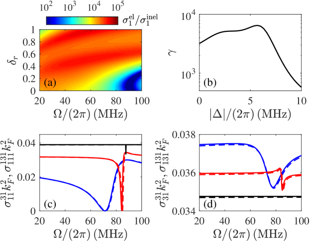
Figure S2: (a) The ratio $\sigma_{1}^{\mathrm{el}}/\sigma_{1}^{\mathrm{inel}}$ for the incident momentum $k_{1}/k_{F}=0.45$. (b) $\gamma$-ratio as a function of the detuning for $T=800\,{\rm nK}$ and $\Omega/(2\pi)=11\,{\rm MHz}$. (c) The scattering cross sections $\sigma_{11}^{31}k_{F}^{2}$ (solid lines) and $\sigma_{111}^{131}k_{F}^{2}$ (dashed lines) as functions of $\Omega$ for $\delta_{r}=0.1$ and $k_{1}/k_{F}=0.04$ (black lines), $0.45$ (red lines), and $1$ (blue lines). (d) The scattering cross sections $\sigma_{31}^{31}k_{F}^{2}$ (solid lines) and $\sigma_{131}^{131}k_{F}^{2}$ (dashed lines) as functions of $\Omega$ for $\delta_{r}=0.1$ and $k_{1}/k_{F}=0.04$ (black lines), $0.45$ (red lines), and $1$ (blue lines).

In Fig. S2, we present additional results on the scattering properties. Figure S2(a) for the incident momentum $k_{1}/k_{F}=0.45$, $\sigma_{1}^{\mathrm{el}}/\sigma_{1}^{\mathrm{inel}}$ shows the small inelastic scattering ($\sigma_{1}^{\mathrm{el}}/\sigma_{1}^{\mathrm{inel}}>10^{3}$) away from the shape resonance (the blue region), which guarantees the projection in the single dressed state channel $\nu=1$. In Fig. S2(b), we plot the $\gamma$-ratio [30] of elastic to inelastic collision rates as a function of $\Delta$ for $\Omega/(2\pi)=11\,{\rm MHz}$, which agrees with the experiment very well. To validate the effective potential $V_{\mathrm{eff}}(\mathbf{r})$, we have shown the good agreement of $\sigma_{11}^{11}$ and $\sigma_{111}^{111}$ in the $p$-wave channel in Fig. 2 of the main text. Here, in Fig. S2(c) and (d), we compare the scattering cross sections $\sigma_{11}^{31}$ with $\sigma_{111}^{131}$ and $\sigma_{31}^{31}$ with $\sigma_{131}^{131}$, respectively. Both exhibit good agreement, which justifies the applicability of $V_{\mathrm{eff}}(\mathbf{r})$.

We also perform calculations using the multi-channel potential and the effective potential S10 for the microwave field with the elliptic angle $\alpha_{m}$, which agree with each other very well for $\alpha_{m}<20^{\circ}$. Remarkably, for a typical experimental setup, even a small elliptic angle, say $\alpha_{m}=5^{\circ}$, can be dramatically reduce the resonance Rabi frequency to about $22\,{\rm MHz}$, a value within the reach of the current experimental technique.

S3 Effective potential in the momentum space

Here we derive the partial wave expansion of the effective potential in the momentum space. To this end, we first note that the Fourier transform of the effective potential is

$$\widetilde{V}_{\mathrm{eff}}(\mathbf{k}-\mathbf{p})=\int d^{3}re^{-i\mathbf{k\cdot r}}V_{\mathrm{eff}}(\mathbf{r})e^{i\mathbf{p\cdot r}}.$$ (S23)

Making use of the partial wave expansion for the plane wave $e^{i\mathbf{k\cdot r}}=4\pi\sum_{lm}i^{l}j_{l}(kr)Y_{lm}(\hat{r})Y_{lm}^{\ast}(\hat{k})$, the effective potential can be expanded as

$$\tilde{V}_{\mathrm{eff}}(\mathbf{k}-\mathbf{p})=(4\pi)^{2}\sum_{ll^{\prime}m}i^{l^{\prime}-l}Y_{lm}(\hat{k})Y_{l^{\prime}m}^{\ast}(\hat{p})\tilde{V}_{ll^{\prime},m}(k,p),$$ (S24)

where

$$\tilde{V}_{ll^{\prime},m}(k,p) =C_{3}\sqrt{\frac{2l^{\prime}+1}{2l+1}}C_{l^{\prime}020}^{l0}C_{l^{\prime}m20}^{lm}v_{3,ll^{\prime}}(k,p)+C_{6}\sqrt{\frac{2l^{\prime}+1}{2l+1}}(7\delta_{ll^{\prime}}-5C_{l^{\prime}020}^{l0}C_{l^{\prime}m20}^{lm}-2C_{l^{\prime}040}^{l0}C_{l^{\prime}m40}^{lm})v_{6,ll^{\prime}}(k,p)$$ (S25)

with

$$v_{s,ll^{\prime}}(k,p)=\int_{0}^{\infty}r^{2}dr\frac{1}{r^{s}}j_{l}(kr)j_{l^{\prime}}(pr).$$ (S26)

For $s=3$ and odd $l$ and $l^{\prime}$, we have

$$v_{3,ll^{\prime}}(k,p)=\left\{\begin{array}[]{ll}\frac{\pi\Gamma\left(\frac{l+l^{\prime}}{2}\right){}_{2}F_{1}\left(\frac{l^{\prime}-l-1}{2},\frac{l+l^{\prime}}{2},\frac{3}{2}+l^{\prime},\frac{p^{2}}{k^{2}}\right)}{8\Gamma\left(\frac{3+l-l^{\prime}}{2}\right)\Gamma\left(\frac{3}{2}+l^{\prime}\right)}\left(\frac{p}{k}\right)^{l^{\prime}},&\mbox{ for }k>p,\\ \frac{\pi\Gamma\left(\frac{l+l^{\prime}}{2}\right){}_{2}F_{1}\left(\frac{l-l^{\prime}-1}{2},\frac{l+l^{\prime}}{2},\frac{3}{2}+l,\frac{k^{2}}{p^{2}}\right)}{8\Gamma\left(\frac{3+l^{\prime}-l}{2}\right)\Gamma\left(\frac{3}{2}+l\right)}\left(\frac{k}{p}\right)^{l},&\mbox{ for }p>k,\end{array}\right.$$ (S29)

which is regular. However, for $s=6$ and odd $l$ and $l^{\prime}$, $v_{6,ll^{\prime}}(k,p)$ becomes divergent when $l=l^{\prime}=1$. To properly treat this divergence, we introduce a short-range cutoff $r_{\mathrm{UV}}$ on the lower integration limit in Eq. (S26), which leads to

$$v_{6,ll^{\prime}}(k,p)=\frac{kp}{9r_{\mathrm{UV}}}\delta_{l1}\delta_{l^{\prime}1}+\left\{\begin{array}[]{ll}\frac{\pi\Gamma\left(\frac{l+l^{\prime}-3}{2}\right){}_{2}F_{1}\left(\frac{l^{\prime}-l}{2}-2,\frac{l+l^{\prime}-3}{2},\frac{3}{2}+l^{\prime},\frac{p^{2}}{k^{2}}\right)}{64\Gamma\left(3+\frac{l-l^{\prime}}{2}\right)\Gamma\left(\frac{3}{2}+l^{\prime}\right)}k^{3}\left(\frac{p}{k}\right)^{l^{\prime}},&\mbox{ for }k>p,\\ \frac{\pi\Gamma\left(\frac{l+l^{\prime}-3}{2}\right){}_{2}F_{1}\left(\frac{l-l^{\prime}}{2}-2,\frac{l+l^{\prime}-3}{2},\frac{3}{2}+l,\frac{k^{2}}{p^{2}}\right)}{64\Gamma\left(3+\frac{l^{\prime}-l}{2}\right)\Gamma\left(\frac{3}{2}+l\right)}p^{3}\left(\frac{k}{p}\right)^{l},&\mbox{ for }p>k.\end{array}\right.$$ (S32)

We use Eq. (S32) throughout our calculations and take the limit $r_{\mathrm{UV}}\rightarrow 0$ as the final step to obtain the result.

References

(1) L. D. Carr, D. DeMille, R. V. Krems, and J. Ye, New J. Phys. 11, 055049 (2009).
(2) S. A. Moses, J. P. Covey, M. T. Miecnikowski, D. S. Jin, and J. Ye, Nature Phys. 13, 13 (2017).
(3) P. Rabl, D. DeMille, J. M. Doyle, M. D. Lukin, R. J. Schoelkopf, and P. Zoller, Phys. Rev. Lett. 97, 033003 (2006).
(4) D. DeMille, Phys. Rev. Lett. 88, 067901 (2002).
(5) R. Sawant, J. A. Blackmore, P. D. Gregory, J. Mur-Petit, D. Jaksch, J. Aldegunde, J. M. Hutson, M. R. Tarbutt, and S. L. Cornish, New J. Phys. 22, 013027 (2020).
(6) A. Micheli, G. Brennen, and P. Zoller, Nature Phys. 2, 341 (2006).
(7) E. Altman et al, PRX Quantum 2, 017003 (2021).
(8) R. V. Krems, Phys. Chem. Chem. Phys. 10, 4079 (2008).
(9) M.-G. Hu, Y. Liu, D. D. Grimes, Y.-W. Lin, A. H. Gheorghe, R. Vexiau, N. Bouloufa-Maafa, O. Dulieu, T. Rosenband, and K.-K. Ni, Science 366, 1111 (2019).
(10) V. V. Flambaum and M. G. Kozlov, Phys. Rev. Lett. 99, 150801 (2007).
(11) T. A. Isaev, S. Hoekstra, and R. Berger, Phys. Rev. A 82, 052521 (2010).
(12) J. J. Hudson, D. M. Kara, I. J. Smallman, B. E. Sauer, M. R. Tarbutt, and E. A. Hinds, Nature (London) 473, 493 (2011).
(13) T. Lahaye, C. Menotti, L. Santos, M. Lewenstein, and T. Pfau, Rep. Prog. Phys. 72, 126401 (2009).
(14) M. A. Baranov, M. Dalmonte, G. Pupillo, and P. Zoller, Chem. Rev. 112, 5012 (2012).
(15) N. J. Fitch and M. R. Tarbutt, Advances in Atomic, Molecular, and Optical Physics 70, 157 (2021).
(16) K.-K. Ni, S. Ospelkaus, M. De Miranda, A. Pe’Er, B. Neyenhuis, J. Zirbel, S. Kotochigova, P. Julienne, D. Jin, and J. Ye, Science 322, 231 (2008).
(17) T. Takekoshi, L. Reichsöllner, A. Schindewolf, J. M. Hutson, C. R. Le Sueur, O. Dulieu, F. Ferlaino, R. Grimm, and H.-C. Nägerl, Phys. Rev. Lett. 113, 205301 (2014).
(18) P. K. Molony, P. D. Gregory, Z. Ji, B. Lu, M. P. Köppinger, C. R. Le Sueur, C. L. Blackley, J. M. Hutson, and S. L. Cornish, Phys. Rev. Lett. 113, 255301 (2014).
(19) J. W. Park, S. A. Will, and M. W. Zwierlein, Phys. Rev. Lett. 114, 205302 (2015).
(20) F. Seesselberg, N. Buchheim, Zhen-Kai Lu, T. Schneider, Xin-Yu Luo, E. Tiemann, I. Bloch, and C. Gohle, Phys. Rev. A 97, 013405 (2018).
(21) K. K. Voges, P. Gersema, M. Meyer zum Alten Borgloh, T. A. Schulze, T. Hartmann, A. Zenesini, and S. Ospelkaus, Phys. Rev. Lett. 125, 083401 (2020).
(22) M. Guo, B. Zhu, B. Lu, X. Ye, F. Wang, R. Vexiau, N. Bouloufa-Maafa, G. Quéméner, O. Dulieu, and D. Wang, Phys. Rev. Lett. 116, 205303 (2016).
(23) T. M. Rvachov, H. Son, A. T. Sommer, S. Ebadi, J. J. Park, M. W. Zwierlein, W. Ketterle, and A. O. Jamison, Phys. Rev. Lett. 119, 143001 (2017).
(24) I. Stevenson, A. Z. Lam, N. Bigagli, C. Warner, W. Yuan, S. Zhang, and S. Wil, arXiv:2206.00652 (2022).
(25) W. B. Cairncross, J. T. Zhang, Lewis R. B. Picard, Yichao Yu, K, Wang, and Kang-Kuen Ni, Phys. Rev. Lett. 126, 123402 (2021).
(26) L. De Marco, G. Valtolina, K. Matsuda, W. G. Tobias, J. P. Covey, and J. Ye, Science 363, 853 (2019).
(27) M. Duda, X.-Y. Chen, A. Schindewolf, R. Bause, J. von Milczewski, R. Schmidt, I. Bloch, and X.-Y. Luo, arXiv:2111.04301 (2021).
(28) G. Valtolina, K. Matsuda, W. G. Tobias, J.-R. Li, L. DeMarco, and J. Ye, Nature 588, 239 (2020).
(29) J.-R. Li, W. G. Tobias, K. Matsuda, C. Miller, G. Valtolina, L. De Marco, R. R. Wang, L. Lassablière, G. Quéméner, J. L. Bohn, and J. Ye, Nat. Phys. 17, 1144 (2021).
(30) A. Schindewolf, R. Bause, X.-Y. Chen, M. Duda, T. Karman, I. Bloch, and X.-Y. Luo, Nature 607, 677 (2022).
(31) K. Matsuda, L. De Marco, J.-R. Li, W. G. Tobias, G. Valtolina, G. Quéméner, and J. Ye, Science 370, 1324 (2020).
(32) L. Anderegg, S. Burchesky, Yicheng Bao, S. S. Yu, T. Karman, E. Chae, Kang-Kuen Ni, W. Ketterle, and J. M. Doyle, Science 373, 779 (2021).
(33) L. You and M. Marinescu, Phys. Rev. A 60, 2324 (1999).
(34) M. A. Baranov, M. S. Mar’enko, Val. S. Rychkov, and G. V. Shlyapnikov, Phys. Rev. A 66, 013606 (2002).
(35) N. R. Cooper and G. V. Shlyapnikov, Phys. Rev. Lett. 103, 155302 (2009).
(36) T. Shi, J.-N. Zhang, C.-P. Sun, and S. Yi, Phys. Rev. A 82, 033623 (2010).
(37) J. Levinsen, N. R. Cooper, and G. V. Shlyapnikov, Phys. Rev. A 84, 013603 (2011).
(38) T. Karman and J. M. Hutson, Phys. Rev. Lett. 121, 163401 (2018).
(39) T. Karman, Z. Z. Yan, and M. Zwierlein, Phys. Rev. A 105, 013321 (2022).
(40) A. V. Avdeenkov and J. L. Bohn, Phys. Rev. Lett. 90, 043006 (2003).
(41) Lucas Lassablière and Goulven Quéméner, Phys. Rev. Lett. 121, 163402 (2018).
(42)B. R. Johnson, J. Comput. Phys. 13, 445 (1973).
(43) M. A. Baranov, L. Dobrek, and M. Lewenstein, Phys. Rev. Lett. 92, 250403 (2004).
(44) K. V. Samokhin and M. S. Mar’enko, Phys. Rev. Lett. 97, 197003 (2006).
(45) C. J. Wu and J. E. Hirsch, Phys. Rev. B 81, 020508(R) (2010).
(46) C. Zhao, L. Jiang, X. Liu, W. M. Liu, X. Zou, and H. Pu, Phys. Rev. A 81, 063642 (2010).
(47) T. Shi, S.-H. Zou, H. Hu, C.-P. Sun, and S. Yi, Phys. Rev. Lett. 110, 045301 (2014).
(48) R. Qi, Z.-Y. Shi, and H. Zhai, Phys. Rev. Lett. 110, 045302 (2013).
(49) See Supplemental Material for a detailed derivation of the effective potential, the numerical procedure for the scattering calculation, and the effective potential in the momentum space.
(50) C. A. R. Sá de Melo, M. Randeria, and Jan R. Engelbrecht
Phys. Rev. Lett. 71, 3202 (1993).
(51) M. Iskin and C. A. R. Sá de Melo, Phys. Rev. Lett. 96, 040402 (2006).
(52) J. P. Gaebler, J. T. Stewart, J. L. Bohn, and D. S. Jin, Phys. Rev. Lett. 98, 200403 (2007).
(53) X.-Y. Chen, A. Schindewolf, S. Eppelt, R. Bause, M. Duda, S. Biswas, T. Karman, T. Hilker, I. Bloch, and X.-Y. Luo, in preparation.