Variational quantum eigensolver for causal loop Feynman diagrams and directed acyclic graphs

Abstract

We present a variational quantum eigensolver (VQE) algorithm for the efficient bootstrapping of the causal representation of multiloop Feynman diagrams in the Loop-Tree Duality (LTD) or, equivalently, the selection of acyclic configurations in directed graphs. A loop Hamiltonian based on the adjacency matrix describing a multiloop topology, and whose different energy levels correspond to the number of cycles, is minimized by VQE to identify the causal or acyclic configurations. The algorithm has been adapted to select multiple degenerated minima and thus achieves higher detection rates. A performance comparison with a Grover’s based algorithm is discussed in detail. The VQE approach requires, in general, fewer qubits and shorter circuits for its implementation, albeit with lesser success rates.

I Introduction

In recent years, there has been a tremendous progress in achieving highly-precise theoretical predictions for particle colliders, which has been possible because of the development of new techniques in Quantum Field Theories (QFT) as well as improved (classical) hardware. For instance, from the theory point of view, the calculation of multiloop scattering amplitudes and Feynman integrals was optimized by applying different sophisticated techniques. Some of these theoretical advancements include Mellin-Barnes transformations Blumlein (2000); Bierenbaum et al. (2006); Gluza et al. (2007); Freitas and Huang (2010); Dubovyk et al. (2016), algebraic reduction of integrands Mastrolia and Ossola (2011); Badger et al. (2012); Zhang (2012); Mastrolia et al. (2012, 2013); Ita (2016); Mastrolia et al. (2016); Ossola et al. (2007), integration-by-parts identities Chetyrkin and Tkachov (1981); Laporta (2000), contour deformation assisted by neural networks Winterhalder et al. (2022) and sector decomposition Binoth and Heinrich (2000); Smirnov and Tentyukov (2009); Carter and Heinrich (2011); Borowka et al. (2018), among several other highly efficient methods. Special emphasis was recently put in the development of four dimensional methods Gnendiger et al. (2017); Heinrich (2021); Torres Bobadilla et al. (2021), with the purpose of achieving a seamless combination of algebraic/analytic strategies and numerical integration directly in the four physical dimensions of the space-time. Overcoming the current precision frontier will certainly require to push these methods to their limits.

Future collider experiments require challenging theoretical predictions from full calculations at order $n$ in the perturbative expansion (NⁿLO), with $n\geq 3$. One foreseeable complication is directly related to the appearance of several scales in multiloop multileg Feynman integrals. These objects are analytically known for specific processes and kinematic configurations up to two loops with a limited number of scales and very few examples of three-loop amplitudes are starting to pop-up Caola et al. (2021a, b). At this point, it is very unlikely that all the required ingredients will become analytically available and the development of novel numerical approaches seems unavoidable.

Given present and future needs, a major progress in solving (at least) two challenges is necessary. On one side, new computational techniques must be developed, exploiting the fundamental properties of QFT and the mathematical concepts behind scattering amplitudes. On the other side, these new methods must be implemented in efficient event generators, capable of overcoming the bottlenecks of the currently available hardware.

Regarding the first challenge, we focus on the Loop-Tree Duality (LTD) formalism Catani et al. (2008); Rodrigo et al. (2008); Bierenbaum et al. (2010, 2013); Buchta et al. (2014, 2017); Buchta (2015); Llanes Jurado et al. (2017); Tomboulis (2017); Plenter (2019); Plenter and Rodrigo (2021); Plenter (2022), which exhibits very attractive mathematical properties and a manifestly causal physical interpretation. Multiloop scattering amplitudes are transformed in LTD into the so-called dual amplitudes by integrating out one component of each of the loop momenta through the Cauchy’s residue theorem. In this way, physical observables are expressed in terms of Euclidean integrals that combine loop and tree-level contributions (as well as renormalization counter-terms) to achieve a fully local cancellation of singularities Hernandez-Pinto et al. (2016); Sborlini et al. (2016a, b); Driencourt-Mangin et al. (2019); Driencourt-Mangin (2019); Driencourt-Mangin et al. (2022); Prisco and Tramontano (2021). Besides the possibility of a local regularization, including the simultaneous cancellation of infrared and ultraviolet singularities, the LTD formalism fully exploits causality in QFT. A recent reformulation Aguilera-Verdugo et al. (2019, 2020a, 2021a); Ramírez-Uribe et al. (2021); Aguilera-Verdugo et al. (2021b); Torres Bobadilla (2021); Sborlini (2021); Bobadilla (2021); Capatti et al. (2019, 2020); Runkel et al. (2019, 2020); Kromin et al. (2022) showed that multiloop scattering amplitudes and Feynman integrals can be represented in terms of a subset of cut diagrams that generalize the well-known Cutkosky’s rules Cutkosky (1960). In particular, a manifestly causal representation can be directly obtained by decomposing the original Feynman diagrams into binary connected partitions in the equivalence class of topologies defined by collapsing propagators into edges (or multi-edges) Sborlini (2021, September 2021). As a result, a well defined geometrical algorithm is available and a strong connection between causality and directed acyclic graphs can be established Ramírez-Uribe et al. (2022).

The other challenge is related to an efficient calculation of Feynman integrals, overcoming current hardware limitations. In this direction, the development of novel strategies for classically hard problems based on quantum algorithms (QAs) is gaining momentum across different areas. For instance, there are several ideas that exploit the potential speed-up of quantum computers, such as database querying through Grover’s algorithm Grover (1997), the famous Shor’s algorithm for factorization of large integers Shor (1997) or Hamiltonian minimization through quantum annealing Kadowaki and Nishimori (1998). In the context of particle physics, QAs are often applied to solve problems related to lattice gauge theories Jordan et al. (2012); Bañuls et al. (2020); Zohar et al. (2016); Byrnes and Yamamoto (2006); Ferguson et al. (2021); Kan et al. (2021). Recent applications for high-energy colliders include jet identification and clustering Wei et al. (2020); Pires et al. (2021, 2020); de Lejarza et al. (2022); Delgado and Thaler (2022); Barata et al. (2022); Barata and Salgado (2021), determination of parton densities (PDFs) Pérez-Salinas et al. (2021), simulation of parton showers Williams et al. (2022); Gustafson et al. (2022), anomaly detection Ngairangbam et al. (2022), and integration of elementary particle processes Agliardi et al. (2022). This list is rapidly growing, since QAs are suitable for several uses, especially those involving minimization problems.

With this panorama in mind, the purpose of this article is to explore the application of QAs for unveiling the causal structure of multiloop scattering amplitudes and Feynman integrals, or equivalently acyclic configurations of directed graphs. Our strategy consists in exploiting the properties of the adjacency matrix in graph theory to build a Hamiltonian which weights the cost of different momentum flow configurations. Explicitly, causal configurations are those with minimum energy, so we select them by identifying the minima of the Hamiltonian. This identification is implemented through a Variational Quantum Eigensolver (VQE) Peruzzo et al. (2014); Mc Clean et al. (2016); Tilly et al. (2022), namely a hybrid quantum-classical algorithm that seeks the ground state of a given operator.

The classical problem of identifying or counting directed acyclic graphs is #P-hard, see Ref. Linial (1986). Explicitly, given a graph $G=(V,E)$ with $V$ vertices and $E$ edges, there are $2^{|E|}$ possible directed graphs that must be checked for cycles. Efficient classical algorithms have been proposed in the literature: e.g., Ref. Oliveira et al. (2019) gives an example of a Fixed Parameter Tractable algorithm, whose scaling depends on a single structural parameter of the graph, see also references therein. This algorithm consists of a Binary Decision Diagram algorithm Bryant (1986), which performs asymptotically in ${\cal O}(2^{p_{w}^{2}/4})$ running time per solution, with the path-width $p_{w}$ always smaller than the input size of the graph, becoming closer to it for dense graphs (i.e., maximally connected graphs). Instead, the motivation of our paper is to encode the complexity of the graph by means of a Hamiltonian, i.e. a cost function to be minimized in order to find the directed acyclic configurations. Since VQE is expected to offer a speed-up in minimization problems compared to purely classical algorithms, we explore up to what extent this speed-up remains in the detection of directed acyclic graphs.

The outline of this paper is the following. In Sec. II, we present a brief introduction to LTD, and we offer a description of its manifestly causal representation. Then, in Sec. III, we discuss the geometrical aspects of the causal configurations, presenting explicit examples in App. A. After that, we introduce the Hamiltonian approach in Sec. IV, putting special emphasis in the connection with the adjacency matrix of directed acyclic graphs. We offer a definition of the loop Hamiltonian and its classical reconstruction algorithm in Secs. IV.1 and IV.2, respectively. We discuss subtleties of the encoding of vertex registers in App. B. Then, we discuss the implementation of the VQE in Sec. V, presenting an explicit example for a representative two-loop topology in Sec. V.1. The full list of Hamiltonians for the topologies studied in this article is given in App. C. Right after in Sec. V.2, we discuss an improved strategy based on multiple runs of the VQE to collect, step by step, all the possible causal solutions. In Sec. VI, we carefully compare the VQE approach with the Grover’s based algorithm described in Ref. Ramírez-Uribe et al. (2022), paying attention to the resources required for a successful implementation in (real) quantum devices. Finally, conclusions and further research directions are presented in Sec. VII.

II Loop-Tree Duality and Causality

To reach highly precise theoretical predictions, it is necessary to deal with multiloop scattering amplitudes and the corresponding Feynman integrals. In the Feynman representation, the most general $L$-loop scattering amplitude with $P$ external particles is given by

$${\cal A}_{F}^{(L)}=\int_{\ell_{1}\ldots\ell_{L}}{\cal N}\big{(}\{\ell_{s}\}_{L},\{p_{j}\}_{P}\big{)}\prod_{i=1}^{n}G_{F}(q_{i})~{},$$ (1)

where $q_{i}$ with $i\in\{1,\ldots,n\}$ are the momenta flowing through each Feynman propagator, $G_{F}(q_{i})=(q_{i}^{2}-m_{i}^{2}+\imath 0)^{-1}$, and ${\cal N}$ represents a numerator, whose specific form depends on the topologies of the different diagrams, the interaction vertices and the nature of the particles that propagate inside the loops. Regarding the momenta of the internal particles, they are linear combinations of the primitive loop momenta associated to the integration variables in the loop, $\ell_{s}$ with $s\in\{1,\ldots,L\}$), and the external momenta, $p_{j}$ with $j\in\{1,\ldots,P\}$. Given a Feynman diagram, we can group the different internal momenta into sets: two lines are said to belong to the same set if their propagators involve the same linear combination of primitive loop momenta Aguilera-Verdugo et al. (2020a). This is useful for achieving an efficient classification of diagrams according to their causal structure Aguilera-Verdugo et al. (2021a); Ramírez-Uribe et al. (2021); Aguilera-Verdugo et al. (2021b).

The denominator of Eq. (1) characterizes the singular structure of the scattering amplitude, and singularities provide important information to simplify loop calculations. In this direction, the Loop-Tree Duality (LTD) Catani et al. (2008); Rodrigo et al. (2008) makes use of Cauchy’s residue theorem (CRT) to reduce the dimensionality of the integration domain, enabling the possibility of transforming it into an Euclidean space. By means of an iterated application of CRT, we can get rid of one integration variable per loop: this is equivalent to say that the LTD representation of a $L$-loop amplitude is obtained by cutting (or setting on-shell) $L$ internal lines. The effect of cutting a line is the modification of the infinitesimal complex prescription, leading to the so-called dual propagators Catani et al. (2008); Rodrigo et al. (2008). It is important to highlight that this modified prescription plays a crucial role to preserve causality, as we will discuss later.

The traditional formulation of LTD leads to the so-called dual representation, in which there is one contribution for each possible connected tree obtained by setting on-shell $L$ internal propagators. If we study the structure of the denominators of each dual term, we immediately realize the presence of divergences that do not correspond to any physical configuration. These unphysical singularities are spurious, and they vanish when we add all the dual contributions together. This is the so called manifestly causal representation within LTD Aguilera-Verdugo et al. (2020a, b).

Before moving on, let us recall one crucial fact about the Feynman propagators. If we define the positive on-shell energy

$$q_{i,0}^{(+)}=\sqrt{\vec{q_{i}}^{2}+m_{i}^{2}-\imath 0}\,,$$ (2)

then the propagator can be written as

$$G_{F}(q_{i})=\frac{1}{q_{i,0}-q_{i,0}^{(+)}}\times\frac{1}{q_{i,0}+q_{i,0}^{(+)}}\,.$$ (3)

This decomposition suggests that each Feynman propagator encodes a quantum superposition of two on-shell modes, with positive and negative energy respectively. The so-called causal representations are obtained by consistently aligning these modes. Furthermore, this superposition also motivates the identification of each internal propagator with a qubit, as we will explain later.

As carefully discussed in Refs. Aguilera-Verdugo et al. (2020a, 2021c), the calculation of the nested residues within the LTD formalism leads to a manifestly causal representation of multiloop multileg scattering amplitudes. Thus, it can be shown that Eq. (1) is equivalent to

$${\cal A}_{D}^{(L)}=\int_{\vec{\ell}_{1}\ldots\vec{\ell}_{L}}\frac{1}{x_{n}}\sum_{\sigma\in\Sigma}{\cal N}_{\sigma}\,\prod_{i=1}^{n-L}\,\frac{1}{\lambda_{\sigma(i)}^{h_{\sigma(i)}}}\ +(\lambda^{+}_{p}\leftrightarrow\lambda^{-}_{p})~{},$$ (4)

with $x_{n}=\prod_{n}2q_{i,0}^{(+)}$, $h_{\sigma(i)}=\pm 1$, and

$$\int_{\vec{\ell}_{s}}=-\mu^{4-d}\int\frac{d^{d-1}\ell_{s}}{(2\pi)^{d-1}}\,,$$ (5)

the integration measure in the loop three-momentum space. It turns out that Eq. (4) only involves denominators with on-shell energies, added together in same-sign combinations within the so-called causal propagators, $1/\lambda_{\sigma(i)}^{h_{\sigma(i)}}$, with

$$\lambda_{\sigma(i)}^{h_{\sigma(i)}}\equiv\lambda_{p}^{\pm}=\sum_{i\in p}q_{i,0}^{(+)}\pm k_{p,0}~{},$$ (6)

where $\sigma(i)$ includes information about the partition $p$ of the set of on-shell energies and the corresponding orientation of the energy components of the external momenta, $k_{p,0}$. Each causal propagator is in a one-to-one correspondence with any possible threshold singularity of the amplitude ${\cal A}_{F}^{(L)}$, which contains overlapped thresholds. These are known as entangled causal thresholds: $\sigma(i)$ indicates the set of causal propagators that can be simultaneously entangled. The set $\Sigma$ in Eq. (4) contains all the combinations of allowed causal entangled thresholds, which involves overlapped cuts with aligned momenta flow.

An important advantage of the representation shown in Eq. (4) is the absence of spurious nonphysical singularities. In fact, since causal propagators involve same-sign combinations of positive on-shell energies, the only possible singularities are related to IR/UV and physical thresholds. More details about the manifestly causal LTD representation and its benefits can be found in Refs. Aguilera-Verdugo et al. (2021a); Ramírez-Uribe et al. (2021); Torres Bobadilla (2021); Sborlini (2021).

III Geometric interpretation of causal flows

In order to identify the causal configurations of a multiloop Feynman diagram in a quantum device, it is necessary to translate the problem into a suitable language. The geometrical formulation of the manifestly causal LTD representations Sborlini (2021) provides a clear and intuitive interpretation. In the following, we briefly describe the most relevant features of this formalism, recalling some basic concepts and definitions as presented in Refs. Ramírez-Uribe et al. (2022); Sborlini (2021, September 2021).

Any scattering amplitude can be represented starting from Feynman diagrams built from interaction vertices and internal lines (or propagators) connecting those vertices. Regarding causality, those lines that connect the same vertices can be merged into a single edge, leading to reduced Feynman graphs because the only allowed configurations which are causal are those in which all the momentum flows of these propagators are aligned in the same direction. Then, reduced graphs are built from vertices and edges, as described in Refs. Torres Bobadilla (2021); Sborlini (2021); Bobadilla (2021), and their causal structure turns out to be equivalent to that of the dual representation of the original Feynman diagrams Aguilera-Verdugo et al. (2021b). The number of loop integration variables in the LTD representation given by Eq. (4) is directly related to the topological independent loops present at the level of the Feynman diagram. However, the reduced Feynman graph has a fewer number of graphical loops, also called eloops, since bunches of propagators connecting the same vertices were collapsed to a single edge. Furthermore, it turns out that vertices, edges and eloops are the only required ingredients to obtain the causal representation of any multiloop scattering amplitude Sborlini (2021); Torres Bobadilla (2021).

Specifically, given a reduced Feynman graph, the associated causal propagators $1/\lambda_{p}^{\pm}$ correspond to the set of connected binary partitions of vertices. Also, they can be graphically interpreted as lines cutting the diagrams into two disconnected pieces, in a full analogy with Cutkosky’s formulation Cutkosky (1960). Then, the representation in Eq. (4) can be constructed from all the possible causal compatible combinations of $k$ causal propagators, the so-called causal entangled thresholds. The number $k$ is known as the order of the diagram and defined as $k=V-1$ Aguilera-Verdugo et al. (2020a); Torres Bobadilla (2021); Sborlini (2021). It naturally induces a topological classification of families of Feynman diagrams, or equivalently, reduced Feynman graphs. The family with $k=1$ is known as Maximal Loop Topology (MLT) Aguilera-Verdugo et al. (2020a) and only involves two vertices; a Next-to-Maximal Loop Topology (NMLT) has three vertices, and so on.

It was shown that causal entangled thresholds can be identified by imposing geometrical selection rules. These rules are deeply connected to the algebraic formulation presented in Refs. Torres Bobadilla (2021); Benincasa and Bobadilla (2022), and they establish that:

1. When considering all the $k$ causal thresholds that can be simultaneously entangled, all the edges can be set on shell simultaneously. This is equivalent to impose that the causal entangled thresholds depends on the on-shell energies $q_{i,0}^{(+)}$ of all the edges.

2. Two different causal propagator $\lambda_{i}$ and $\lambda_{j}$ can be simultaneously entangled if they do not cross each other. In other words, this means that the associated partition of vertices do not intersect or are totally included one in the other.

3. The momentum of the edges that crosses a given binary partition of vertices must be consistently aligned, i.e., momentum must flow from one partition to a different one.

A careful explanation of these causal rules and their geometric interpretation was presented in Ref. Sborlini (2021), including pedagogical examples and practical cases of use. By imposing these three rules on the set of all the possible combinations of $k$ thresholds, we construct $\Sigma$, namely the set of all causal entangled thresholds leading to Eq. (4). Furthermore, as previously shown in Ref. Ramírez-Uribe et al. (2022), the third condition is equivalent to ordering the internal edges in such a way that the reduced Feynman diagram is a directed acyclic graph. This means that there cannot be closed cycles, allowing the information to propagate consistently from one partition of the diagram to the other; this condition is necessary for having a causal-compatible partition. For this reason, given a reduced Feynman graph, it is crucial to efficiently detect all the associated directed acyclic graphs, since they are a vital ingredient to reconstruct the LTD causal representation. To clarify this discussion, we present an explicit application example in App. A.

IV Hamiltonian formalism for causal-flow identification

The first proof-of-concept of a quantum algorithm for Feynman loop integrals was presented in Ref. Ramírez-Uribe et al. (2022), managing to successfully unfold the causal configurations of multiloop Feynman diagrams. The implementation follows a modified Grover’s quantum algorithm to identify the presence of directed acyclic configurations, representing the causal solutions, over different subloops of the multiloop topologies.

The aim of this Section is to define a Hamiltonian whose ground state corresponds to a superposition of all the acyclic configurations of a given multiloop Feynman diagram. We first discuss the construction of such Hamiltonian based on direct inspection of the multiloop topology, and then we discuss a more general approach based on the adjacency matrix of a graph, an object that concentrates all the information regarding the orientation of edges and the vertices that they connect within a reduced Feynman graph (as defined in Sec. III). We also give a more formal presentation, relying on concepts and notations from graph theory.

IV.1 Cycle detection via Hamiltonian optimization

Let us consider a generic undirected graph $G=(V,E)$, with $V$ a set of distinct vertices and $E\subset V\times V$ a set of edges (also known as links). Given the graph $G$, one can build a set $\mathcal{D}_{G}$ of $2^{|E|}$ possible directed graphs where we associate a specific direction to each link. We will denote the subset of directed acyclic graphs as $\widetilde{\mathcal{D}}_{G}\subset\mathcal{D}_{G}$.

In order to formulate this problem as a Hamiltonian optimization, we first fix the encoding for all the possible (classical) solutions as elements of the computational basis as follows. We start by establishing a conventional orientation to each edge, selecting a specific element from the set of directed graphs $G_{0}\in\mathcal{D}_{G}$. This set is associated to the state $|{00\dots 0}\rangle\in\mathcal{H}_{E}$, mapping each qubit to an edge as done in Ref. Ramírez-Uribe et al. (2022): the single qubit state $|{0}\rangle_{e}$ for the edge $e\in E$ corresponds to a link with the same orientation of $e$ in the conventional graph $G_{0}$, while the state $|{1}\rangle_{e}$ would correspond to the opposite orientation. The problem can then be cast in the search of all the possible states of the computational basis of edge orientations associated to directed acyclic graphs $\widetilde{\mathcal{D}}_{G}$, whose span generates a Hilbert space $\widetilde{\mathcal{H}}_{E}\subset\mathcal{H}_{E}$.

After these definitions, we need to identify the set $\Gamma_{G_{0}}$ of all the possible oriented cycles. In this notation, the subscript $G_{0}$ means that we will use the reference graph to specify the orientations of those cycles. Here, cycle refers to simple cycles (i.e. a closed loop in which a vertex appears only once). If the set $\Gamma_{G_{0}}$ of directed loops is already known, one can build the so-called loop Hamiltonian, which is a Hamiltonian on the space $\mathcal{H}_{E}$, diagonal in the computational basis described above. We proceed by penalizing oriented cycles using diagonal projectors, i.e.

$$H_{G}=\sum_{\gamma\in\Gamma_{G_{0}}}\prod_{e\in\gamma}\pi^{s(e;G_{0})}_{e}~{},$$ (7)

where $s(e;G_{0})$ evaluates to $0$ or $1$ according to the orientation of $e\in\gamma$ relative to the conventional graph orientation $G_{0}$, and the $\pi$ symbol identifies the projector operators on single edge registers,

$$\pi^{0}_{e} \equiv|{0}\rangle\langle{0}|_{e}=\frac{1}{2}{(I+Z)}_{e}~{},$$ (8)

$$\pi^{1}_{e} \equiv|{1}\rangle\langle{1}|_{e}=\frac{1}{2}{(I-Z)}_{e}~{},$$

with $Z$ the Pauli matrix in the $z$-axis.

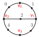
FIG. 1: Example of a diagram with two eloops and four vertices representing external particles (Topology A). Edges are directly numbered, and vertices are explicitly indicated as $v_{i}$.

To provide an explicit example, let us consider Fig. 1. It depicts a graph $G_{0}$ (i.e., $G$ equipped with a conventional orientation), where one can identify by direct inspection the set of all the possible directed loops:

$$\Gamma_{G_{0}}=\Big{\{} \big{[}\bar{0},2,\bar{1}\big{]},\big{[}0,\bar{2},1\big{]},\big{[}4,3,2\big{]},[\bar{4},\bar{3},\bar{2}\big{]},$$

$$\big{[}1,4,3,0\big{]},\big{[}\bar{1},\bar{4},\bar{3},\bar{0}\big{]}\Big{\}}~{},$$ (9)

where the presence or absence of the bar identifies the orientation (i.e., $s(e,G_{0})=0$, $s(\bar{e},G_{0})=1$). Then, the loop Hamiltonian has the following form:

$$H_{G} =\pi^{1}_{0}\pi^{0}_{2}\pi^{1}_{1}+\pi^{0}_{0}\pi^{1}_{2}\pi^{0}_{1}+\pi^{0}_{4}\pi^{0}_{3}\pi^{0}_{2}$$

$$+\pi^{1}_{4}\pi^{1}_{3}\pi^{1}_{2}+\pi^{0}_{1}\pi^{0}_{4}\pi^{0}_{3}\pi^{0}_{0}+\pi^{1}_{1}\pi^{1}_{4}\pi^{1}_{3}\pi^{1}_{0}.$$ (10)

Notice that a term in $H_{G}$ acts trivially on a non-indicated edge, i.e.

$$\pi^{1}_{0}\pi^{0}_{2}\pi^{1}_{1}\equiv I_{4}\otimes I_{3}\otimes\pi^{0}_{2}\otimes\pi^{1}_{1}\otimes\pi^{1}_{0}\,,$$ (11)

with $I_{i}$ corresponding to the identity operator on ${\cal H}_{i}$. This loop Hamiltonian will evaluate to $0$ for any solution in $\widetilde{\mathcal{D}}_{G}$ of graphs without oriented cycles (i.e., $\operatorname{Ker}(H_{G})=\widetilde{\mathcal{H}}_{E}$), while the other directed graphs are associated to a strictly greater than $0$ integer eigenvalue. Moreover, the same oriented graph could have more than one closed cycle, and this Hamiltonian counts the number of these oriented cycles.

IV.2 Classical algorithm for reconstructing the loop Hamiltonian

The adjacency matrix of a graph provides a powerful tool to further characterise the associated multiloop topology, and it can be used when the loop set is not straightforward to compute. Classically, the adjacency matrix $A=||a||$ of a directed graph of $N=|V|$ vertices (labelled in an arbitrary manner) is defined such that $a_{i_{1}i_{2}}=1$ ($i_{1},i_{2}=1,\ldots,N$) if there is a directed edge from $i_{1}$ to $i_{2}$, and $0$ otherwise. Note that a cycle of length $\ell$ along the vertices $i_{0},\ldots,i_{\ell-1},i_{\ell}=i_{0}$ implies $a_{i_{0}i_{1}}\times\ldots\times a_{i_{\ell-1}i_{\ell}}=1$. Moreover, if $A\in\mathbb{Z}_{2}^{N\times N}$, the following properties are equivalent:

1. the graph of which $A$ is the adjacency matrix is acyclic;

2. $A^{N}=0$, i.e. $A$ is nilpotent (which is stronger than $\text{tr}(A^{N})=0$);

3. $A$ is equivalent to a triangular matrix, where equivalence has a precise algebraic meaning, corresponding to the existence of a relabelling;

4. the eigenvalues of $A$ are all zero, which directly implies $\text{tr}(A^{k})=0$ for any positive integer $k$.

We can exploit these equivalent properties to build suitable candidates for Hamiltonians. For this purpose, let us consider a graph $G=(V,E)$ and a corresponding conventionally oriented graph $G_{0}=(V,\bar{E})$. Then, we define an extended Hilbert space of vertices and edges $\mathcal{H}_{VE}\equiv\mathcal{H}_{V}\times\mathcal{H}_{E}$, and we build a linear operator acting on it and encoding the information about the oriented adjacency matrix:

$$A\equiv\sum_{e\equiv(v_{0},v_{1})\in\bar{E}}\Big{[}\sigma^{-}_{v_{0}}\pi^{0}_{e}\sigma^{+}_{v_{1}}+\sigma^{-}_{v_{1}}\pi^{1}_{e}\sigma^{+}_{v_{0}}\Big{]}\,,$$ (12)

where $\sigma^{\pm}=(X\pm i\,Y)/2$ are the ladder operators. This construction can be interpreted as a sum of hopping terms from the tail to the head vertices of each oriented edge $e$, with the edge projector operators $\pi^{s}_{e}$ keeping track of the orientation relative to the conventional graph. Thus, joining two adjacent edges would give nontrivial contributions only if the orientation is the same for both edges (i.e., if the head of one is joined with the tail of the other), and that is ensured by the properties of the ladder operators on the corresponding vertex register. Therefore, the $n$-th power of the $A$ operator will have non-zero diagonal terms in the vertex side only if all the ladder operators are completely contracted and only projectors $\pi^{s}$ appear. On the edge side, these terms identify oriented cycles (or disjoint products of oriented cycles), so that a possible loop Hamiltonian, whose kernel is the span of directed acyclic graph states $\widetilde{\mathcal{H}}_{E}$, can be written as follows:

$$H_{G}=\sum\limits_{n=1}^{M_{G}}\text{tr}(A^{n})\,,$$ (13)

where the trace runs only over the vertex space, and $M_{G}$ is the maximal length of loops in $G$, i.e., $M_{G}=|V|$. An oriented cycle going across $j$ vertices corresponds to a term in this sum when $n=j$. The loop Hamiltonian built in this way has the same terms as the loop Hamiltonian in Eq. (7), plus some terms representing disjoint products of oriented cycles (e.g., two oriented cycles going respectively across $j_{1}$ and $j_{2}$ vertices and corresponding to a term in the sum above when $n=j_{1}+j_{2}$). Also, it includes coefficients in front of the different products of projectors $\pi$, which are related to topological properties of the graph under consideration (see, e.g., Eq. (V) below). In any case, the ground state will be associated with the subspace of directed acyclic graphs. For the practical implementation, we will rely on the normalized version of $H_{G}$ where all the coefficients in front of the $\pi$ operators are exactly 1.

It is worth mentioning that, to derive a loop Hamiltonian, in principle any positive-definite function of $A$ can be used. For example,

$$H^{\prime}_{G}=\text{tr}(e^{A}-I)\,,$$ (14)

would have a different spectrum, but exactly the same kernel as the loop Hamiltonian in Eq. (13). Given the relation ${\rm tr}(A^{j})=\sum^{N}_{i=1}\lambda^{j}_{i}$, where $\lambda_{i}$ ($i=1,\ldots,N$) are the eigenvalues of the adjacency matrix, one sees that cycles are deeply connected to spectral properties of graphs. So, the problem we have at hand consists in knowing whether any of these eigenvalues is non-zero, in which case cycles would be present. Since the Hamiltonians defined above are related to the eigenvalues, they are independent of the specific labelling of the graph in consideration.

To conclude this section, note that a discussion about efficient encoding methods for the vertex space is presented in App. B, having in mind the possibility of a Hamiltonian reconstruction by means of a purely quantum algorithm. Also, we would like to mention that the number of terms in the loop Hamiltonian does not depend on the number of external legs. As shown in App. C, more complex topologies require more terms because each term of the Hamiltonian penalizes the presence of cycles. Thus, more loops leads to more possible cycles to be checked, and this translates into more terms in the Hamiltonian, but more external legs do not generate additional cycles. Computing the Hamiltonian in a fully quantum way, as we discuss in App. B, could allow to speed-up the codification of the characteristics of the graph for the posterior minimization with a quantum device.

V VQE implementation and numerical results

We now discuss the application of the Variational Quantum Eigensolver (VQE) algorithm Peruzzo et al. (2014); Mc Clean et al. (2016) to find directed acyclic graphs given a fixed topology. Fixing a positive orientation for an arbitrary link (the first one for example), the $|E|-1$ remaining qubits encode the direction of the other links, i.e., the states considered have the form $|{\psi}\rangle\otimes|{0}\rangle$ with the restricted loop Hamiltonian $H_{E/\{e_{0}\}}\equiv H_{E}\rvert_{s(e_{0},G_{0})=0}$ acting only on $|{\psi}\rangle$. This is possible without loss of generality, since the solutions to the unrestricted problem can be found by adding a copy of the solutions to the restricted problem $\{|{\psi_{j}}\rangle\}\subset\widetilde{\mathcal{H}}_{E/\{e_{0}\}}\cap\mathbb{Z}_{2}^{|E|-1}$ with all links flipped:

$$\big{\{}|{\psi_{j}}\rangle\otimes|{0}\rangle\big{\}}\cup\big{\{}\big{(}X^{\otimes{(|E|-1)}}|{\psi_{j}}\rangle\big{)}\otimes|{1}\rangle\big{\}}\subset\widetilde{\mathcal{H}}_{E}\cap\mathbb{Z}_{2}^{|E|}\,,$$ (15)

where $\big{(}X^{\otimes{(|E|-1)}}|{\psi_{j}}\rangle\big{)}$ corresponds to applying a tensor product of NOT gates to the first $|E|-1$ bits to invert the directions of the links/edges described in $|{\psi_{j}}\rangle$.

To explain how the proposed algorithm works, let us consider again the topology shown in Fig. 1, where $|E|=5$. The unrestricted Hamiltonian obtained from Eq. (13) is

$$H_{E} =3\pi_{0}^{1}\,\pi_{1}^{1}\,\pi_{2}^{0}\,+3\pi_{0}^{0}\,\pi_{1}^{0}\,\pi_{2}^{1}\,+4\pi_{0}^{0}\,\pi_{1}^{0}\,\pi_{3}^{0}\,\pi_{4}^{0}\,$$

$$+3\pi_{2}^{0}\,\pi_{3}^{0}\,\pi_{4}^{0}\,+4\pi_{0}^{1}\,\pi_{1}^{1}\,\pi_{3}^{1}\,\pi_{4}^{1}\,+3\pi_{2}^{1}\,\pi_{3}^{1}\,\pi_{4}^{1}\,\,\,,$$ (16)

where we point out the presence of nontrivial coefficients in front of each term, that results from having identical terms in Eq. (13). As explained before, the ground state will have always 0 energy and it will be associated to the set of directed acyclic graphs, independently of the spectrum of $H_{E}$. For the sake of simplicity, from now on, we will work with the normalized Hamiltonian, eliminating the positive coefficients seen in Eq. (V).

Then, we can fix the orientation of the first qubit in agreement with the initial choice which implies

$$\pi_{0}^{0}|{\psi}\rangle=|{\psi}\rangle\,,\quad\pi_{0}^{1}|{\psi}\rangle=0\,,$$ (17)

with $|{\psi}\rangle\in\{|{\psi^{\prime}}\rangle\otimes|{0}\rangle\}$. This is equivalent to set $\pi_{0}^{0}\equiv I_{0}$ and remove all the terms proportional to $\pi_{0}^{1}$. Explicitly

$$H_{E/\{e_{0}\}} =\pi_{1}^{0}\,\pi_{2}^{1}\,+\pi_{1}^{0}\,\pi_{3}^{0}\,\pi_{4}^{0}\,$$

$$+\pi_{2}^{0}\,\pi_{3}^{0}\,\pi_{4}^{0}\,+\pi_{2}^{1}\,\pi_{3}^{1}\,\pi_{4}^{1}\,,$$ (18)

which acts over the reduced edge space. The computational basis of the restricted problem represents the $2^{|E|-1}=16$ possible directed graphs, of which only $9$ are acyclic (i.e., the solutions to our minimization problem). In practice, all the $9$ solutions of the reduced problem can be found by applying the VQE where we minimize $\langle{H_{E/\{e_{0}\}}}\rangle$ with any of the Hamiltonians built as discussed in the previous sections. As argued above, the space of solutions corresponds to the intersection between the canonical basis and the eigenspace associated with the eigenvalue $0$. A single run of the VQE converging to $\langle{H_{E/\{e_{0}\}}}\rangle=0$ (within precision), will, in general, result in a superposition of states of the computational basis in $\operatorname{Ker}H_{E/\{e_{0}\}}$. In analogy to the Grover’s approach, we collect solutions whose probability appears above a certain threshold $\lambda$. However, in this case, there is no guarantee that all possible solutions are found in the superposition of a single run. In the following, we will explain a possible strategy to overcome this difficulty, based on running the VQE multiple times.

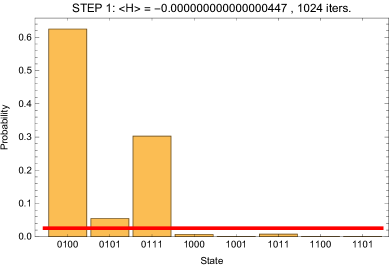
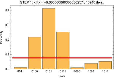
FIG. 2: Approximation of the ground state found by VQE with COBYLA optimizer, corresponding to the two-eloop diagram in Fig. 1. We present the probability of the different states contributing to the ground state after 1024 (left) and 10240 (right) iterations with 1024 shots. The red line is a threshold to limit the contamination by noncausal configurations.

V.1 Example: two-eloop case

Now, we concentrate again our attention to the explicit example of Fig. 1. As a first step, we proceed to translate Eq. (18) to the basis of Pauli operators using the definition of the projectors given in Eq. (8). The result is

$$H_{E/\{e_{0}\}} =4\,I_{4}\otimes I_{3}\otimes I_{2}\otimes I_{1}+2\,I_{4}\otimes I_{3}\otimes I_{2}\otimes Z_{1}$$

$$-I_{4}\otimes I_{3}\otimes Z_{2}\otimes I_{1}-I_{4}\otimes I_{3}\otimes Z_{2}\otimes Z_{1}$$

$$+I_{4}\otimes Z_{3}\otimes I_{2}\otimes I_{1}+I_{4}\otimes Z_{3}\otimes I_{2}\otimes Z_{1}$$

$$+2\,I_{4}\otimes Z_{3}\otimes Z_{2}\otimes I_{1}+Z_{4}\otimes I_{3}\otimes I_{2}\otimes I_{1}$$

$$+Z_{4}\otimes I_{3}\otimes I_{2}\otimes Z_{1}+2\,Z_{4}\otimes I_{3}\otimes Z_{2}\otimes I_{1}$$

$$+3\,Z_{4}\otimes Z_{3}\otimes I_{2}\otimes I_{1}+Z_{4}\otimes Z_{3}\otimes I_{2}\otimes Z_{1}~{}.$$ (19)

Then, we setup the VQE using the package qiskit.algorithms together with the function RealAmplitudes to generate the Ansätze. In this experiment, we use the optimizer COBYLA Powell (1994), with maxiter=$\{$1024,10240$\}$, and the simulation is implemented in the aer$\_$simulator with a fixed number of shots (by default shots=1024). Notice that iterations refers to the number of times that the classical optimization algorithm is called. This has to be distinguished from shots, which is the number of times the quantum circuit is executed and measured. In any case, we observe that more iterations allow to achieve a better convergence of the optimization whilst more shots are associated with a more precise determination of the mean value of the Hamiltonian.

In Fig. 2, we show the probability of the different configurations contributing to the approximate ground state. The yellow bars are associated to acyclic (or causal) configurations, that the algorithm is aimed to identify. For the present topology, there are 9 acyclic configurations in the reduced space, namely:

$$\big{\{} |{0011}\rangle,\ |{0100}\rangle,\ |{0101}\rangle,\ |{0111}\rangle,\$$

$$|{1000}\rangle,\ |{1001}\rangle,\ |{1011}\rangle,\ |{1100}\rangle,\ |{1101}\rangle\big{\}}\,.$$ (20)

In this particular example, the simulation leads to the identification of 3 solutions, for both maxiter$=1024$ and maxiter$=10240$. The extremely good approximation to the exact energy of the ground state implies in practice that there was no contamination with noncausal configurations. However, this is not guaranteed, as we will see in subsequent examples along the article. Furthermore, we notice that a single VQE run (i.e., the set of quantum and classical steps discussed so far, which includes a certain number of shots and iterations) is generally not enough to collect all the solutions of the problem. Since there are several local minima, the minimization algorithm could be stuck in one of them and achieve convergence without exploring the full set of possibilities. The situation is even more complicated because there are multiple degenerated global minima, whose contribution to the ground state can be re-scaled arbitrarily without changing the energy. This implies that the random selection of the initial points might produce very different probability distributions from run to run: in other words, if we re-run the experiment, it is highly probable that the distributions in Fig. 2 change substantially, selecting a different subset of causal solutions. For these reasons, we define the success rate as

$$r_{\rm success}=\frac{\#(\rm{total\ detected})}{\#(\rm{causal\ total})\times\big{(}1+\#(\rm{incorrect\ states})\big{)}}\,,$$ (21)

which also takes into account the possibility of misidentification of causal states. For the particular example presented in Fig. 2, we have $r_{\rm success}=0.89$ and $r_{\rm success}=0.78$, respectively. If we increase the number of iterations, we find the results in Fig. 3: we have $r_{\rm success}=0.56$ for maxiter$=102400$ and $r_{\rm success}=1$ for maxiter$=1024000$ iterations. In the first case, one of the states, $|{0110}\rangle$, is noncausal, which leads to the drastic decrease of the success rate.

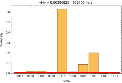
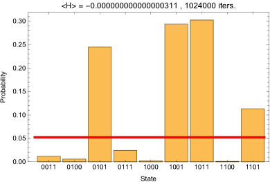
FIG. 3: Approximation of the ground state found by VQE with COBYLA optimizer, corresponding to the two-eloop diagram in Fig. 1. We present the probability of the different states contributing to the ground state after 102400 (left) and 1024000 (right) iterations, with 1024 shots. The red line is a threshold to limit the contamination by noncausal configurations.

With the purpose of reducing the probability of collecting incorrect states, we can select only those states contributing to the approximated ground state with a probability above a certain threshold $\lambda$. Since the VQE is optimized to find the states with lower energy, it is reasonable to assume that there are much higher probabilities to include acyclic rather than noncausal configurations in the approximated ground state. Thus, if the solution found by VQE is

$$|{\psi_{0}}\rangle=\sum_{j}c_{j}|{\phi_{j}}\rangle\,,$$ (22)

then we propose the threshold $\lambda$ to be

$$\lambda=\max\left(\,\overline{(|c_{j}|^{2})}-\frac{\Delta(|c_{j}|^{2})}{2},\min(|c_{j}|^{2})\,\right)\,,$$ (23)

i.e. the average minus a term proportional to the standard deviation of the probabilities $|c_{j}|^{2}$, or the minimum of such probabilities. This value of $\lambda$ corresponds to the red line in Figs. 2 and 3. We would like to emphasize that this definition is empirical, and motivated by the exploration of the numerical results. Also, if we want to increase the certainty that only causal states are selected, we can take higher values of $\lambda$. This could eventually lead to a lower success rate (since more states are rejected). To balance this situation, we can run multiple times the VQE procedure and collect solutions in each step until we fulfill a certain convergence criterion, discussed in the next section.

To conclude this section, we would like to mention that different versions of the optimizers and Ansätze were used. In particular, besides COBYLA, we performed the optimization with SPSA Spall (1998) and NFT Nakanishi et al. (2020), achieving similar results. However, COBYLA turned out to run faster on our computer. Regarding the Ansatz, we relied on RealAmplitudes and EfficientSU2, both circuits being part of qiskit.circuit.library. Again, the success rates for the topology A of Fig. 1 were rather similar, although RealAmplitudes involves half of the parameters of EfficientSU2. However, the use of RealAmplitudes manifests into slightly higher values of the Hamiltonian mean value. Moreover, as we will see in the next section, it was necessary at times to switch to EfficientSU2 to avoid missing solutions, while also avoiding misidentifications.

V.2 Multiple-run VQE approach

In order to find the complete set of solutions, one can set up a sequence of VQE runs where the Hamiltonian used contains additional terms which suppress the solutions found at each previous step of the sequence. The proposed theoretical algorithm is the following:

1. We start with the reduced Hamiltonian $H^{(0)}=H_{E/\{e_{0}\}}$ and apply the VQE algorithm using an Ansatz. We can choose as an initial point the uniform superposition of all the configurations, i.e.

   $$|{\psi^{(0)}}\rangle=\sqrt{2^{1-|E|}}\,\sum_{i}|{\phi_{i}}\rangle\,,$$ (24)

   with $\{|{\phi_{i}}\rangle\}$ the canonical basis of the reduced edge space ${\cal H}_{E/\{e_{0}\}}$.

2. The VQE minimization is executed till it finds a state with energy $E_{1}<\tilde{\mu}$ or until the maximum number of iterations, maxiter, is reached. In case the energy condition is not fulfilled, we run the VQE again till it converges to $E_{1}<\tilde{\mu}$ (which is guaranteed by the presence of, at least, 1 causal configuration). The approximation to the ground state is expressed as

   $$|{\psi^{(1)}}\rangle=\sum_{j}c_{j}^{(1)}|{\phi_{j}}\rangle\,.$$ (25)

3. We pick up the subset ${\cal S}_{1}=\{|{\phi_{j}}\rangle\,|\,|c_{j}^{(1)}|^{2}>\lambda\}$, which corresponds to elements with a high probability of belonging to $\operatorname{Ker}H_{E/\{e_{0}\}}$. Then, we define a penalization term to exclude these potential solutions from the next run. Explicitly, we consider

   $$\Pi^{(1)}=\sum_{|{\phi_{l}}\rangle\in{\cal S}_{1}}b^{(1)}_{l}|{\phi_{l}}\rangle\langle{\phi_{l}}|\,,$$ (26)

   with $b_{l}^{(1)}$ positive coefficients to be set appropriately. Steps 1-3 define the single-run VQE, used in Sec. V.1.

4. We define the modified reduced Hamiltonian

   $$H^{(1)}=H^{(0)}+\Pi^{(1)}\,,$$ (27)

   and re-run the VQE. If it does not find any state such that $E_{2}<\tilde{\mu}$ within the given allowed number of iterations, then the algorithm stops. The set of solutions remains ${\cal S}={\cal S}_{1}$.

5. If a state

   $$|{\psi^{(2)}}\rangle=\sum_{j}c_{j}^{(2)}|{\phi_{j}}\rangle\,,$$ (28)

   such that $E_{2}<\tilde{\mu}$ is found, then we pick up the set ${\cal S}_{2}=\{|{\phi_{j}}\rangle\,|\,|c_{j}^{(2)}|^{2}>\lambda\}$, build the associated penalization term $\Pi^{(2)}$ and add ${\cal S}_{2}$ to the set of solutions.

6. Repeat Step 4 and 5 till the algorithm stops when the mean energy is greater than $\tilde{\mu}$.

This approach is rather general and can be modified by adjusting several parameters: we can choose different energy thresholds $\tilde{\mu}$ for each step, different Ansätze, probability thresholds, modify the number of shots and/or classical iterations for each VQE run, etc.. Although in the next section, we will discuss some of these observations, we defer a more detailed study for future works. Also, we would like to point out that this procedure does not guarantee collecting all the solutions. Due to the presence of so-called barren plateaus McClean et al. (2018), the VQE could get stuck around local minima which do not belong to the true ground-state. This is a shared drawback of several minimization strategies (including VQE), in which the presence of large regions in the parameter space with rather small gradients prevents an efficient optimization Sack et al. (2022). In the next section, we discuss improvements to overcome barren plateaus and increase the success rate, keeping a very low error rate.

Also, in the VQE literature Fedorov et al. (2021), it is normally highlighted the importance of choosing a suitable Ansatz that properly represents at least the low-lying eigenstates of the Hamiltonian. In the context of quantum chemistry, this is usually possible since the Hamiltonians represent physical systems and analytical approximations or mathematical properties of the solutions are known. By choosing an appropriate Ansatz it would be possible to achieve a faster convergence and partially avoid the barren plateaus. However, in our case, the situation is not straightforward and identifying an optimal Ansatz is far from trivial. The choice of the Ansatz in general should have parametrized rotational gates and one or more layers of entanglement to be able to connect the qubits, if the entanglement entropy of the system is not zero. So, for finding convergence in this particular problem, it is enough to have a generic circuit structure. Our approach can be considered as a first exploration, and further investigations in this direction will be performed in the future.

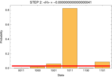
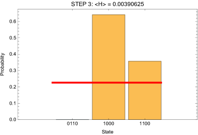
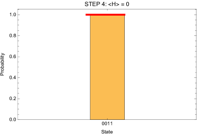
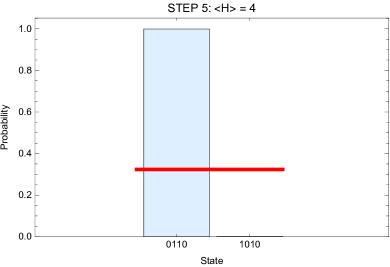
FIG. 4: Iterated application of the VQE with COBYLA optimizer, corresponding to the two-eloop diagram in Fig. 1. We present the probability of the different states contributing to the ground state after 1024 iterations. States in yellow (light-blue) represent causal (noncausal) solutions. The red line is a threshold to limit the contamination by noncausal configurations, described in the text. The algorithm converges after 4 runs.

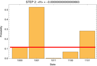
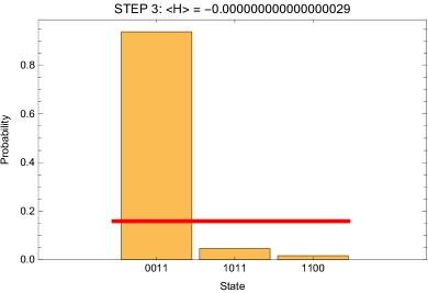
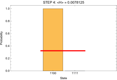
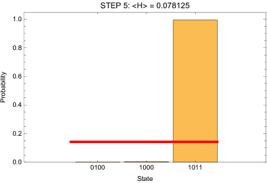
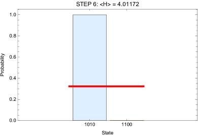
FIG. 5: Iterated application of the VQE with COBYLA optimizer, corresponding to the two-eloop diagram in Fig. 1. We present the probability of the different states contributing to the ground state after 10240 iterations. States in yellow (light-blue) represent causal (noncausal) solutions. The red line is a threshold to limit the contamination by noncausal configurations, described in the text. The algorithm converges after 5 runs.

Now, let us consider again the example of Fig. 1, keeping the two test scenarios (i.e. the ones with 1024 and 10240 iterations, respectively). The starting point is the set of solutions collected from Fig. 2. We set the detection threshold $\lambda$ according to Eq. (23), and we iterate the VQE excluding the solutions found in the precedent step, as in Eq. (27). In Figs. 4 and 5, we present the probabilities of the different states contributing to the approximated ground state, for 1024 and 10240 iterations respectively. In each run, we collect the solutions above the threshold only if the energy is below $\tilde{\mu}=0.1$. In both cases, we manage to successfully identify the 9 causal states, after 5 and 6 runs, for maxiter$=1024$ and maxiter$=10240$ respectively. No misidentification took place because the selection threshold turned out to be rather rigorous. By lowering $\lambda$, the procedure converges faster, but there is an increased risk to pick up a noncausal state.

Before concluding this section, let us briefly discuss the complexity of this approach. Again, the multi-run VQE strategy involves a hybrid classical-quantum setup. On one side, there is a polynomial computational cost for calculating the Hamiltonian, which is ${\cal O}(|V|^{4})$ based on Eq. (13), i.e., distinct $|V|$ rows and $|V|$ columns have to be multiplied, at a cost of $|V|$ per multiplication, and this has to be repeated a total of $|V|-1$ times when $n=|V|$. Then, this Hamiltonian has to be evaluated in a quantum system, leading to a potential speed-up since all the expectation values (i.e., one for each term; see, e.g., Eq. (19)) are simultaneously computed on a superposition of many configurations Tilly et al. (2022). After that, a classical parameter optimization is performed with standardised algorithms (such as COBYLA or NFT) and the procedure is iterated.

VI Comparing Hamiltonian optimization with Grover’s algorithm

After a careful study of the Hamiltonian minimization through VQE, we carry out in this Section a performance comparison with Grover’s based algorithm Ramírez-Uribe et al. (2022). We rely on the set of six representative topologies shown in Fig. 6. These topologies allow us to understand how the quantum circuits’ complexity scales with the number of vertices and edges. In Appendix C, we show the explicit form of the Hamiltonians in $\mathcal{H}_{E}$ for the aforementioned topologies, so that a classical verification of the procedure explained in Sec. IV can be implemented.

FIG. 6: Representative topologies used for the performance comparison of Grover’s and VQE implementations. We considered the following configurations: (A) two eloops with four vertices; (B) three eloops with four vertices; and (C) four eloops with five vertices. Also, we include the complete set of four-eloop six-vertex topologies: (D) $t$-channel; (E) $s$-channel; and (F) $u$-channel.

For each topology, we study the set of causal/acyclic configurations comparing with the output of a classical algorithm. We used the success rate defined in Eq. (21) to quantify the accuracy of the identification of causal states. Then, we compare:

1. the number of qubits required to run the algorithm;

2. the quantum depth of the transpiled circuits;

3. the total number of executions needed to get the full solution.

The first point is important since most of the current quantum devices have a (relatively) small number of qubits. Of course, we expect that this limitation will be overcome in the (near) future, but still it is a tangible drawback. In the same direction, physical bottlenecks to ensure the stability of the qubits prevents to implement very deep circuits. So, from the point of view of the hardware requirements, avoiding a fast growth of these two aspects is crucial to ensure the feasibility of the quantum approach. Finally, the third point implies more execution time, since re-running the circuit implies preparing the state and repeating the measurements. However, this is not a hard limiting factor as the previous two properties, although it penalizes the performance.

A further comment is needed to explain the definition of quantum depth and executions in this comparison. Regarding the quantum depth, it is related to the number of operations or quantum gates that are involved within the circuit. Each specific device has a set of fundamental gates, and any other gate/operator is defined by a combination of the fundamental set. As a consequence, the real depth of the circuit is hardware- or simulator- dependent, so we need to fix a convention to compare Grover’s and VQE approaches. Since the calculations are implemented in Qiskit, we use the function qiskit.compiler.transpile and aer$\_$simulator as target device. Then, we estimate the quantum depth through the .depth() method. For the case of Grover’s algorithm, the depth depends not only on the complexity of the topology but also on the number of iterations: for the topologies studied in this article, we can achieve a perfect reconstruction with only one iteration Ramírez-Uribe et al. (2022). Note that in this case, the complexity of the oracle and the diffuser are included. The quantum depth for VQE is related to the complexity of the Ansatz and the Hamiltonian. In fact, for the VQE, we estimate the depth by applying the .depth() method to the circuit composed by one term of the Hamiltonian applied to the Ansatz. So, in general, VQE involves shorter circuits, as discussed in e.g. Tilly et al. (2022).

About the concept of executions, it is directly related to the number of times that we need to measure the output. In the case of Grover’s algorithm, this quantity exactly agrees with the number of shots Grover (1998); Ramírez-Uribe et al. (2022). However, VQE requires a deeper analysis. We need to remember that the VQE pipeline mixes a classical and a quantum algorithm. The quantum circuits depend on parameters, that are adjusted after performing the measurement in order to minimise a certain cost function Tilly et al. (2022). For each choice of parameters, we define a quantum circuit and execute $s$ shots (controlled by the parameter shots within the backend). Then, we allow the algorithm to modify the parameters $r$ times (until the cost function evaluates under a certain threshold), which is what we call an iteration (controlled by maxiterations within the classical optimizer routine). So, each run of the VQE requires $s\times r$ measurements. On top of that, the multiple-run VQE algorithm explained in Sec. V must be repeated $k$ times, adding in each repetition a certain number of penalization terms to the Hamiltonian. As a consequence, we will need to make $s\times r\times k$ executions to complete the identification of the winning states (or causal configurations). For these reasons, in general, VQE involves a larger number of executions compared to Grover’s approach.

Topology	Causal/Total	Success rate	$\#$ Qubits	Quantum depth	$\#$ Executions
A	18/32	100 $\%$	14	35	100
B	24/64	100 $\%$	19	43	100
C	78/256	100 $\%$	25	55	400
D	204/512	100 $\%$	28	62	1300
E	204/512	100 $\%$	28	62	1300
F	230/512	100 $\%$	33	28	1600

Table 1: Performance of the Grover-based algorithm applied to the representative multiloop topologies depicted in Fig. 6

Topology	Causal/Total	Success rate	$\#$ Qubits	Quantum depth	$\#$ Executions
A	18/32	60.7 - 79.1 $\%$	4	7	1000 $\times$ 100
B	24/64	23.9 - 56.8 $\%$	5	9	1000 $\times$ 1000
C	78/256	7.9 - 37.6 $\%$	7	13	1000 $\times$ 1000
D	204/512	3.5 - 35.4 $\%$	8	15	10000 $\times$ 1000
E	204/512	4.0 - 30.5 $\%$	8	15	10000 $\times$ 1000
F	230/512	4.6 - 34.6 $\%$	8	15	10000 $\times$ 1000

Table 2: Performance of the Hamiltonian minimization through VQE applied to the representative multiloop topologies depicted in Fig. 6, using a single run. We indicate the number of executions as shots times iterations. The success rate $r_{\rm success}$ range contemplates the worst case scenario (no threshold, all the states are selected) and the best one (optimal threshold for distinguishing causal from noncausal). Thus, these results illustrate the need for defining a threshold to avoid misidentifications.

Topology	Causal/Total	Success rate	$\#$ Qubits	Quantum depth	$\#$ Runs
A	18/32	88 $\%$	4	7	3
B	24/64	50 $\%$	5	9	4
C	78/256	51 $\%$	7	13	7
D	204/512	34.3 $\%$	8	15	7
E	204/512	43.1 $\%$	8	15	11
F	230/512	44.3 $\%$	8	15	9

Table 3: Performance of the Hamiltonian minimization through VQE applied to the representative multiloop topologies depicted in Fig. 6, using the iterative approach explained in Sec. V. We used 1000 iterations and 1000 shots in each VQE run, with the Setup 2. Even if the success rate was below 100 $\%$, no misidentification took place.

Topology	Causal/Total	Success rate	$\#$ Qubits	Quantum depth	$\#$ Runs
A	18/32	100 $\%$	4	9	3
B	24/64	100 $\%$	5	11	9
C	78/256	97.4 $\%$	7	15	18
D	204/512	93.1 $\%$	8	17	41
E	204/512	95.1 $\%$	8	17	40
F	230/512	87.0 $\%$	8	17	37

Table 4: Performance of the Hamiltonian minimization through VQE applied to the representative multiloop topologies depicted in Fig. 6, using the iterative approach explained in Sec. V. We used 1000 iterations and 1000 shots in each VQE run, with the Setup 3. A major improvement compared to Setup 2 was reached, keeping a null error rate.

In Tables 1 and 2, we present the number of qubits, executions and the quantum depth of the circuits involved in the implementation of the Grover’s algorithm and the single-run VQE approach, respectively, for all the topologies shown in Fig. 6. In the case of Grover, the success rate is 100 $\%$ because we are using the optimal number of executions explored in Ref. Ramírez-Uribe et al. (2022), which guarantees in practice a perfect casual/noncausal discrimination, in spite of requiring more qubits and larger coherence. For the single-run VQE, we estimate the success rate by using Eq. (21). We rely on COBYLA optimizer and RealAmplitudes Ansatz which represents less quantum resources with respect to Grover’s implementation but involves more shots, classical iterations and the efficiency is noticeably smaller. This is because, in the experiments that we executed to obtain the inferior values in the success rate ranges of Tab. 2, we are collecting all the states in the approximate ground-state as solutions of our problem. However, if the energy is not 0 (or compatible with 0 within machine error), this ground-state might be contaminated with noncausal configurations; this will reduce the success rate since we are penalizing the misidentification with Eq. (21). This illustrates the need for defining a proper threshold to retain only the true minima from the approximated ground-state.

Then, we tested the performance of the multiple-run VQE algorithm. We considered different scenarios:

1. Setup 1: COBYLA optimizer with 1000 iterations, 1000 shots, RealAmplitudes with a random parameter initialization as Ansatz and the threshold $\lambda$ given by Eq. (23).

2. Setup 2: NFT optimizer with 1000 iterations, 1000 shots, RealAmplitudes with a random parameter initialization as Ansatz. The selection threshold for the $i$-th run is given by

   $$\lambda_{i}=\max\left(\,\overline{(|c^{(i)}_{j}|^{2})}-\frac{\Delta(|c^{(i)}_{j}|^{2})}{2},\frac{1}{\#{\cal S}_{i}}\,\right)\,,$$ (29)

   if $E_{i}>10^{-8}$, and $\lambda_{i}=0$ otherwise (i.e. if the mean energy of the approximated ground-state is compatible with 0, then all the states are solutions).

3. Setup 3: NFT optimizer with 1000 iterations, 1000 shots, EfficientSU2 using the approximated solution found in the previous run as initial point of its subsequent run. The selection threshold is defined as in Setup 2, and we repeat 3 times the execution of the VQE if $E_{i}>\tilde{\mu}$ in the $i$-th run.

Setup 1 corresponds to the configuration tested in Sec. V.2. We do not present a table with explicit results for complex topologies (such as D, E of F) because the success rates are rather low, even below ${\cal O}(10\,\%)$. This is due to several withdraws of this naive implementation, namely some limitations of COBYLA optimizer and the initial Ansatz. For this reason, we tried other configurations, tweaking the parameters of the multi-run VQE to achieve higher success rates. In Tabs. 3 and 4, we present the results for Setup 2 and Setup 3 respectively. We observe that NFT identifies approximations to the real ground-state with lower energy but with less configurations in superposition w.r.t. COBYLA. In fact, with COBYLA the identification rate could reach up to ${\cal O}(50\%)$, but there are several incorrect states, which leads to very low success rates, see Eq. (21). In contrast, the combination of the NFT optimization and the improved selection threshold from Eq. (29) has an extremely low misidentification rate: in all the topologies tested, the error rate was absent, but each run collects a smaller number of solutions. The difference in the performance is due to the nature of the optimization algorithm. NFT is an optimization method specifically designed for quantum-classical hybrid algorithms based on parameterized quantum circuits, whilst COBYLA is a more general approach envisaged for problems where the derivative of the objective function is unknown. Since it assumes certain properties of the cost function, NFT allows to reach configurations with lower energy by performing fewer measurements. Even if we were unable to test the performance of these two approaches in real quantum devices, we expect NFT to perform better for the multi-run VQE since it is also claimed to be more effective in the presence of noise (as well as SPSA). Still, in general, it is not clear from first principles which is the best choice of optimizer and, most of the times, this is found by empirical exploration.

Still, in presence of barren plateaus, the implementation in Setup 2 stops before identifying all the possible solutions, since the algorithm gets stuck around local minima. To overcome this limitation, in Setup 3, we consider a more flexible Ansatz and select an optimized value for the initial point. Also, we implemented a routine to randomly kick the parameters when the energy is higher than $\tilde{\mu}=1$ (which means a non-global minimum was found). In this way, we avoid a premature interruption of the multi-run VQE, which keeps collecting solutions, with null error rate.

VII Conclusions and outlook

The computation of accurate theoretical predictions for current and future high-energy particle colliders requires efficient ways to deal with scattering amplitudes at higher orders in the perturbative expansion. In the present article, we put forward a quantum strategy to re-cast the selection of causal configurations of multiloop Feynman integrands into a minimization problem. For this purpose, we exploit the geometrical approach to the causal Loop-Tree Duality (LTD) representation of Feynman integrals Sborlini (2021) and relate causality with the identification of directed acyclic graphs Ramírez-Uribe et al. (2022).

We rely on the concept of adjacency matrix in graph theory to define the so-called loop Hamiltonian, whose different energy levels correspond to graph configurations with different number of cycles. By construction, the ground-state is directly associated to the subspace of states related to directed acyclic graphs. In this way, given a multiloop Feynman diagram, we fix a reference orientation of the internal propagators and then define the associated loop Hamiltonian. By construction, this loop Hamiltonian has mean value 0 when evaluated on acyclic states. Therefore by minimizing the energy, we automatically detect the subset of causal configuration.

After explaining the construction of the loop Hamiltonian, we proceed to solve with quantum minimization algorithms. We use the Variational Quantum Eigensolver (VQE) within the Qiskit framework to test the different configurations. In particular, we develop a multi-run VQE strategy that allows to achieve higher detection rates. The VQE approach is compared against the Grover’s detection procedure implemented in Ref. Ramírez-Uribe et al. (2022). Our results indicate that even if VQE requires less quantum resources than Grover’s algorithm (i.e. it involves fewer qubits and shorter circuits), still a larger number of executions must be performed in order to achieve high success rates. However, since VQE is a hybrid algorithm that employs classical optimization, it allows to use classical hardware and save quantum resources. Given the current limitations in quantum hardware, VQE approach allows to study complex multiloop topologies that would require a prohibitive number of stable qubits within Grover’s implementation.

In conclusion, along this article, we have presented a proof-of-principle for the detection of causal configurations using a loop Hamiltonian implemented in VQE. We have demonstrated the feasibility of our approach, paving the road to achieve an efficient causal reconstruction of multiloop Feynman amplitudes through quantum algorithms using less hardware resources. We have presented a multiple-run VQE algorithm with much better success rates than a naive single-run VQE. We stress that we avoid the misidentification of solutions, reaching null error rates in the simulators. Still, the success rates achieved are not as satisfactory as the ones achieved with a Grover-based algorithm and further investigation is required to develop a better strategy through quantum minimization. In any case, we successfully tested, for the first time, a VQE-based strategy to solve a problem with highly-degenerated ground-states, which constitutes a hard stress-test for this kind of minimization algorithms. A promising road to enhance the success rate and reduce the number of VQE runs is Conditional-Value-at-Risk (CVaR) Barkoutsos et al. (2020), which has already shown improved performance on certain practical problems, such as the allocation of flight gates Stollenwerk et al. (2019); Chai et al. (2023). Also, different strategies must be explored regarding optimal state-preparation, since several results point towards a significant impact of the state-preparation in the performance of the minimization Bravyi et al. (2020); Sun et al. (2023). In particular, it would be highly interesting to test our algorithms in quantum annealers, which could lead to an improved performance and much higher success rates with a lower consumption of quantum resources. We defer these improvements and studies for future investigations.

Appendix A Illustrative application of geometrical causal rules

In Sec. III, we briefly mentioned how to determine the causal entangled thresholds by following geometrical selection rules. Let us consider the diagram shown in Fig. 1 as an illustrative example of the bootstrapping of the causal representation. We will closely follow Refs. Sborlini (September 2021, 2021), together with the concepts exposed in Refs. Aguilera-Verdugo et al. (2020a, 2021a, 2021c); Torres Bobadilla (2021).

The first step consists in the identification of the causal thresholds or causal propagators, which corresponds to connected binary partitions of the set of vertices. The diagram Fig. 1 has $V=4$ vertices connected by $E=5$ edges, which produces a set of 6 causal propagators

$$\lambda_{i+1} = \{v_{i}\}\quad{\rm for}\,i=\{0,\ldots,3\}\,,$$ (30)

$$\lambda_{5} = \{v_{0},v_{1}\}\,,$$ (31)

$$\lambda_{6} = \{v_{0},v_{2}\}\,.$$ (32)

Each $\lambda_{p}$ is graphically indicated by a line crossing the edges that enclose the selected vertices; we will call them causal cuts, since they cut the diagram into two connected ones. For instance, $\lambda_{1}$ corresponds to a line crossing the edges $\{e_{0},e_{1}\}$ and enclosing the vertex $v_{0}$. Furthermore, as explained in Refs. Aguilera-Verdugo et al. (2020a); Sborlini (2021), we define $\lambda_{p}^{+}$ ($\lambda_{p}^{-}$) if all the edges are taken outgoing from (incoming to) the partition defined by $\lambda_{p}$.

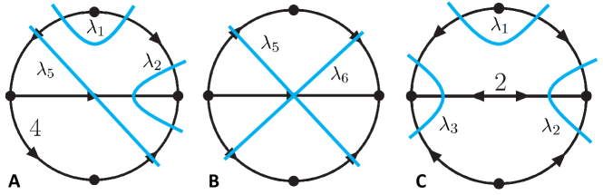
FIG. 7: Graphical interpretation from causal geometrical selection rules of the two-eloop topology from Fig. 1. Although all configurations depicted are acyclic, the selected thresholds are not causally entangled because: (A) not all the edges are cut and the momentum flows in $\lambda_{5}$ are not aligned in the same direction; (B) $\lambda_{5}$ and $\lambda_{6}$ cross each other; and (C) the momentum of $e_{2}$ can not be consistently oriented.

The second step corresponds to the determination of the causal entangled thresholds. Since this diagram has $V=4$, it is of order $k=V-1=3$, that implies that the causal representation is obtained by multiplying 3 causal propagators. Equivalently, it means that the diagram can be decomposed by simultaneously imposing 3 different causal cuts. In principle, there are 20 possibilities but the conditions 1-3 listed in Sec. III limit them to 10. Explicitly, we have

$$\Sigma=\big{\{} \{1,2,4\},\{1,2,6\},\{1,3,4\},\{1,3,5\},\{1,4,5\},$$

$$\{1,4,6\},\{2,3,5\},\{2,3,6\},\{2,4,5\},\{3,4,6\}\big{\}}~{},$$ (33)

where we use the simplified notation $\lambda_{i}\lambda_{j}\lambda_{k}\equiv\{i,j,k\}$. Examples of partitions that are not causally entangled are:

1. $\{1,2,5\}$ is not allowed because $e_{4}$ remains uncut, i.e. condition 1 is not fulfilled.

2. entangled thresholds containing $\{5,6\}$ are not allowed because $\lambda_{5}$ and $\lambda_{6}$ cross each other, i.e. condition 2 is not fulfilled.

3. $\{1,2,3\}$ is not allowed because $e_{2}$ can not be oriented in a consistent way. Explicitly, if we take $\lambda_{1}^{+}$, then we have $\lambda_{2}^{-}$ and $\lambda_{3}^{-}$; but $\lambda_{2}^{-}$ implies $S(e_{2},G_{0})=0$ and $\lambda_{3}^{-}$ implies $S(e_{2},G_{0})=1$ (following the notation introduced in Sec. IV).

These 3 cases are depicted in Fig. 7. Finally, we would like to close this Appendix by reminding that conditions 1-3 are equivalent to the following ones:

1. The edges must be oriented in such a way that cyclic loops are not present, i.e. we need to identify all the possible directed acyclic graphs obtained from the original reduced Feynman graph.

2. Then, we need to dress the acyclic graphs with $k=V-1$ simultaneous causal propagators, in such a way that the conditions 1-2 from the list in Sec. III are fulfilled.

This was the strategy first used in Ref. Ramírez-Uribe et al. (2022) to bootstrap the causal representation, and justifies the importance of developing an efficient algorithm to detect directed acyclic configurations for a given topology.

Appendix B Compact encoding of vertex registers

Having in mind the extension of the VQE algorithm presented in this paper to complex multiloop topologies, it is relevant to think about suitable scaling techniques. As we already know from Ref. Ramírez-Uribe et al. (2022), the number of qubits required to implement the computation scales very fast with the complexity of the underlying graphs. For this, it is important to identify strategies that allow us to reduce the qubit consumption.

One source of proliferation of qubits is associated with the description of the vertex space $V$. The encoding used for the vertex registers in the discussion above is of the one-hot kind, i.e., each classical vertex state for a specific vertex with label $v\in\{0,\dots,|V|-1\}$ is associated to a unique string with all $0$’s except for a single $1$ on the $v$-th position. For example, the vertices in Fig. 1 are associated to the following elements of the computational basis:

$$v_{0} \mapsto|{0001}\rangle_{V};$$ (34)

$$v_{1} \mapsto|{0010}\rangle_{V};$$

$$v_{2} \mapsto|{0100}\rangle_{V};$$

$$v_{3} \mapsto|{1000}\rangle_{V}.$$

With this encoding, the oriented link $e_{(i,j)}:v_{i}\rightarrow v_{j}$ is represented by an hopping term $\sigma^{-}_{v_{i}}\sigma^{+}_{v_{j}}\pi^{0}_{e_{(i,j)}}$. However, it is simpler (and more scalable) to consider a compact encoding using $q=\lceil\log_{2}(|V|)\rceil$ qubits instead of the $|V|$ necessary in the one-hot case. Returning to the example in Fig. 1, one can use a possible compact encoding with just $q=2$ qubits, as the following:

$$v_{0} \mapsto|{00}\rangle_{V};$$ (35)

$$v_{1} \mapsto|{01}\rangle_{V};$$

$$v_{2} \mapsto|{10}\rangle_{V};$$

$$v_{3} \mapsto|{11}\rangle_{V}.$$

The hopping terms for the adjacency matrix can be computed, as for the one-hot encoding, by looking at the oriented link $e_{(i,j)}:v_{i}\rightarrow v_{j}$, which will contain a mix of ladder (at least one) and projector operators. Using Fig. 1, the oriented link $e_{(1,0)}:v_{1}\rightarrow v_{0}$ is associated with the non-Hermitian operator

$$|{00}\rangle\langle{01}|_{V}\otimes\pi^{0}_{e_{(1,0)}}={(\sigma^{-}_{1}\otimes\sigma^{+}_{0})}_{V}\otimes\pi^{0}_{e_{(1,0)}}\,.$$ (36)

After computing all the terms for the operator representing the adjacency matrix $A$, one can build the loop Hamiltonian by tracing out the vertex register as in Eqs. (13)-(14) (or any equivalent positive semi-definite matrix with $\widetilde{\mathcal{H}}_{E}$ as kernel). This is guaranteed by the fact that the only terms contributing to $H_{G}$ after computing the trace are those in $A^{n}$ that do not contain ladder operators (i.e., diagonal terms), because these can be obtained only if the products of the $n$ hopping terms connect the same vertex as input (e.g., $|{v_{i}}\rangle\langle{v_{i}}|_{V}$). In other words, the terms present in $A^{n}$ are those representing a closed chain, starting and ending in the same vertex.

Appendix C Loop Hamiltonians for representative multiloop topologies

In this appendix, we include the formulae for the loop Hamiltonians for the multiloop topologies described in Fig. 6. Results for diagram A were discussed in detail in Sec. V.1, so here we present only expressions for the remaining topologies. Explicitly, we have for diagram B (three eloops with four vertices, or Mercedes diagram),

$$H_{\rm Top.B} =3\pi_{0}^{0}\,\pi_{1}^{0}\,\pi_{2}^{0}\,+3\pi_{0}^{1}\,\pi_{1}^{1}\,\pi_{2}^{1}\,+3\pi_{0}^{1}\,\pi_{3}^{1}\,\pi_{4}^{0}\,$$

$$+4\pi_{1}^{0}\,\pi_{2}^{0}\,\pi_{3}^{1}\,\pi_{4}^{0}\,+3\pi_{0}^{0}\,\pi_{3}^{0}\,\pi_{4}^{1}\,+4\pi_{1}^{1}\,\pi_{2}^{1}\,\pi_{3}^{0}\,\pi_{4}^{1}\,$$

$$+4\pi_{0}^{1}\,\pi_{1}^{1}\,\pi_{3}^{1}\,\pi_{5}^{0}\,+3\pi_{2}^{0}\,\pi_{3}^{1}\,\pi_{5}^{0}\,+3\pi_{1}^{1}\,\pi_{4}^{1}\,\pi_{5}^{0}\,$$

$$+4\pi_{0}^{0}\,\pi_{2}^{0}\,\pi_{4}^{1}\,\pi_{5}^{0}\,+4\pi_{0}^{0}\,\pi_{1}^{0}\,\pi_{3}^{0}\,\pi_{5}^{1}\,+3\pi_{2}^{1}\,\pi_{3}^{0}\,\pi_{5}^{1}\,$$

$$+3\pi_{1}^{0}\,\pi_{4}^{0}\,\pi_{5}^{1}\,+4\pi_{0}^{1}\,\pi_{2}^{1}\,\pi_{4}^{0}\,\pi_{5}^{1}\,,$$ (37)

for diagram C (four eloops with five vertices, or pizza diagram),

$$H_{\rm Top.C} =4\pi_{0}^{0}\,\pi_{1}^{0}\,\pi_{2}^{0}\,\pi_{3}^{0}\,+4\pi_{0}^{1}\,\pi_{1}^{1}\,\pi_{2}^{1}\,\pi_{3}^{1}\,+3\pi_{0}^{1}\,\pi_{4}^{1}\,\pi_{5}^{0}\,$$

$$+5\pi_{1}^{0}\,\pi_{2}^{0}\,\pi_{3}^{0}\,\pi_{4}^{1}\,\pi_{5}^{0}\,+3\pi_{0}^{0}\,\pi_{4}^{0}\,\pi_{5}^{1}\,+5\pi_{1}^{1}\,\pi_{2}^{1}\,\pi_{3}^{1}\,\pi_{4}^{0}\,\pi_{5}^{1}\,$$

$$+4\pi_{0}^{1}\,\pi_{1}^{1}\,\pi_{4}^{1}\,\pi_{6}^{0}\,+4\pi_{2}^{0}\,\pi_{3}^{0}\,\pi_{4}^{1}\,\pi_{6}^{0}\,+3\pi_{1}^{1}\,\pi_{5}^{1}\,\pi_{6}^{0}\,$$

$$+5\pi_{0}^{0}\,\pi_{2}^{0}\,\pi_{3}^{0}\,\pi_{5}^{1}\,\pi_{6}^{0}\,+4\pi_{0}^{0}\,\pi_{1}^{0}\,\pi_{4}^{0}\,\pi_{6}^{1}\,+4\pi_{2}^{1}\,\pi_{3}^{1}\,\pi_{4}^{0}\,\pi_{6}^{1}\,$$

$$+3\pi_{1}^{0}\,\pi_{5}^{0}\,\pi_{6}^{1}\,+5\pi_{0}^{1}\,\pi_{2}^{1}\,\pi_{3}^{1}\,\pi_{5}^{0}\,\pi_{6}^{1}\,+5\pi_{0}^{1}\,\pi_{1}^{1}\,\pi_{2}^{1}\,\pi_{4}^{1}\,\pi_{7}^{0}\,$$

$$+3\pi_{3}^{0}\,\pi_{4}^{1}\,\pi_{7}^{0}\,+4\pi_{1}^{1}\,\pi_{2}^{1}\,\pi_{5}^{1}\,\pi_{7}^{0}\,+4\pi_{0}^{0}\,\pi_{3}^{0}\,\pi_{5}^{1}\,\pi_{7}^{0}\,$$

$$+3\pi_{2}^{1}\,\pi_{6}^{1}\,\pi_{7}^{0}\,+5\pi_{0}^{0}\,\pi_{1}^{0}\,\pi_{3}^{0}\,\pi_{6}^{1}\,\pi_{7}^{0}\,+5\pi_{0}^{0}\,\pi_{1}^{0}\,\pi_{2}^{0}\,\pi_{4}^{0}\,\pi_{7}^{1}\,$$

$$+3\pi_{3}^{1}\,\pi_{4}^{0}\,\pi_{7}^{1}\,+4\pi_{1}^{0}\,\pi_{2}^{0}\,\pi_{5}^{0}\,\pi_{7}^{1}\,+4\pi_{0}^{1}\,\pi_{3}^{1}\,\pi_{5}^{0}\,\pi_{7}^{1}\,$$

$$+3\pi_{2}^{0}\,\pi_{6}^{0}\,\pi_{7}^{1}\,+5\pi_{0}^{1}\,\pi_{1}^{1}\,\pi_{3}^{1}\,\pi_{6}^{0}\,\pi_{7}^{1}\,,$$ (38)

for diagram D (four eloops with six-vertices in $t$-channel configuration),

$$H_{\rm Top.D}=4\pi_{0}^{0}\,\pi_{1}^{0}\,\pi_{2}^{0}\,\pi_{3}^{0}\,+4\pi_{0}^{1}\,\pi_{1}^{1}\,\pi_{2}^{1}\,\pi_{3}^{1}\,+6\pi_{1}^{1}\,\pi_{5}^{1}\,\pi_{6}^{0}\,$$

$$+5\pi_{0}^{0}\,\pi_{2}^{0}\,\pi_{3}^{0}\,\pi_{5}^{1}\,\pi_{6}^{0}\,+6\pi_{1}^{0}\,\pi_{5}^{0}\,\pi_{6}^{1}\,+5\pi_{0}^{1}\,\pi_{2}^{1}\,\pi_{3}^{1}\,\pi_{5}^{0}\,\pi_{6}^{1}\,$$

$$+5\pi_{0}^{1}\,\pi_{1}^{1}\,\pi_{2}^{1}\,\pi_{4}^{1}\,\pi_{7}^{0}\,+6\pi_{3}^{0}\,\pi_{4}^{1}\,\pi_{7}^{0}\,+6\pi_{0}^{1}\,\pi_{2}^{1}\,\pi_{4}^{1}\,\pi_{5}^{0}\,\pi_{6}^{1}\,\pi_{7}^{0}\,$$

$$+5\pi_{0}^{0}\,\pi_{1}^{0}\,\pi_{2}^{0}\,\pi_{4}^{0}\,\pi_{7}^{1}\,+6\pi_{3}^{1}\,\pi_{4}^{0}\,\pi_{7}^{1}\,+6\pi_{0}^{0}\,\pi_{2}^{0}\,\pi_{4}^{0}\,\pi_{5}^{1}\,\pi_{6}^{0}\,\pi_{7}^{1}\,$$

$$+4\pi_{0}^{1}\,\pi_{4}^{1}\,\pi_{5}^{0}\,\pi_{8}^{0}\,+6\pi_{1}^{0}\,\pi_{2}^{0}\,\pi_{3}^{0}\,\pi_{4}^{1}\,\pi_{5}^{0}\,\pi_{8}^{0}\,+5\pi_{0}^{1}\,\pi_{1}^{1}\,\pi_{4}^{1}\,\pi_{6}^{0}\,\pi_{8}^{0}\,$$

$$+5\pi_{2}^{0}\,\pi_{3}^{0}\,\pi_{4}^{1}\,\pi_{6}^{0}\,\pi_{8}^{0}\,+5\pi_{1}^{0}\,\pi_{2}^{0}\,\pi_{5}^{0}\,\pi_{7}^{1}\,\pi_{8}^{0}\,+5\pi_{0}^{1}\,\pi_{3}^{1}\,\pi_{5}^{0}\,\pi_{7}^{1}\,\pi_{8}^{0}\,$$

$$+4\pi_{2}^{0}\,\pi_{6}^{0}\,\pi_{7}^{1}\,\pi_{8}^{0}\,+6\pi_{0}^{1}\,\pi_{1}^{1}\,\pi_{3}^{1}\,\pi_{6}^{0}\,\pi_{7}^{1}\,\pi_{8}^{0}\,+4\pi_{0}^{0}\,\pi_{4}^{0}\,\pi_{5}^{1}\,\pi_{8}^{1}\,$$

$$+6\pi_{1}^{1}\,\pi_{2}^{1}\,\pi_{3}^{1}\,\pi_{4}^{0}\,\pi_{5}^{1}\,\pi_{8}^{1}\,+5\pi_{0}^{0}\,\pi_{1}^{0}\,\pi_{4}^{0}\,\pi_{6}^{1}\,\pi_{8}^{1}\,+5\pi_{2}^{1}\,\pi_{3}^{1}\,\pi_{4}^{0}\,\pi_{6}^{1}\,\pi_{8}^{1}\,$$

$$+5\pi_{1}^{1}\,\pi_{2}^{1}\,\pi_{5}^{1}\,\pi_{7}^{0}\,\pi_{8}^{1}\,+5\pi_{0}^{0}\,\pi_{3}^{0}\,\pi_{5}^{1}\,\pi_{7}^{0}\,\pi_{8}^{1}\,+4\pi_{2}^{1}\,\pi_{6}^{1}\,\pi_{7}^{0}\,\pi_{8}^{1}\,$$

$$+6\pi_{0}^{0}\,\pi_{1}^{0}\,\pi_{3}^{0}\,\pi_{6}^{1}\,\pi_{7}^{0}\,\pi_{8}^{1}\,,$$ (39)

for diagram E (four eloops with six-vertices in $s$-channel configuration),

$$H_{\rm Top.E}=4\pi_{0}^{0}\,\pi_{1}^{0}\,\pi_{2}^{0}\,\pi_{3}^{0}\,+4\pi_{0}^{1}\,\pi_{1}^{1}\,\pi_{2}^{1}\,\pi_{3}^{1}\,+6\pi_{0}^{1}\,\pi_{4}^{1}\,\pi_{5}^{0}\,$$

$$+5\pi_{1}^{0}\,\pi_{2}^{0}\,\pi_{3}^{0}\,\pi_{4}^{1}\,\pi_{5}^{0}\,+6\pi_{0}^{0}\,\pi_{4}^{0}\,\pi_{5}^{1}\,+5\pi_{1}^{1}\,\pi_{2}^{1}\,\pi_{3}^{1}\,\pi_{4}^{0}\,\pi_{5}^{1}\,$$

$$+6\pi_{2}^{1}\,\pi_{6}^{1}\,\pi_{7}^{0}\,+5\pi_{0}^{0}\,\pi_{1}^{0}\,\pi_{3}^{0}\,\pi_{6}^{1}\,\pi_{7}^{0}\,+6\pi_{1}^{0}\,\pi_{3}^{0}\,\pi_{4}^{1}\,\pi_{5}^{0}\,\pi_{6}^{1}\,\pi_{7}^{0}\,$$

$$+6\pi_{2}^{0}\,\pi_{6}^{0}\,\pi_{7}^{1}\,+5\pi_{0}^{1}\,\pi_{1}^{1}\,\pi_{3}^{1}\,\pi_{6}^{0}\,\pi_{7}^{1}\,+6\pi_{1}^{1}\,\pi_{3}^{1}\,\pi_{4}^{0}\,\pi_{5}^{1}\,\pi_{6}^{0}\,\pi_{7}^{1}\,$$

$$+5\pi_{0}^{0}\,\pi_{1}^{0}\,\pi_{4}^{0}\,\pi_{6}^{1}\,\pi_{8}^{0}\,+5\pi_{2}^{1}\,\pi_{3}^{1}\,\pi_{4}^{0}\,\pi_{6}^{1}\,\pi_{8}^{0}\,+4\pi_{1}^{0}\,\pi_{5}^{0}\,\pi_{6}^{1}\,\pi_{8}^{0}\,$$

$$+6\pi_{0}^{1}\,\pi_{2}^{1}\,\pi_{3}^{1}\,\pi_{5}^{0}\,\pi_{6}^{1}\,\pi_{8}^{0}\,+6\pi_{0}^{0}\,\pi_{1}^{0}\,\pi_{2}^{0}\,\pi_{4}^{0}\,\pi_{7}^{1}\,\pi_{8}^{0}\,+4\pi_{3}^{1}\,\pi_{4}^{0}\,\pi_{7}^{1}\,\pi_{8}^{0}\,$$

$$+5\pi_{1}^{0}\,\pi_{2}^{0}\,\pi_{5}^{0}\,\pi_{7}^{1}\,\pi_{8}^{0}\,+5\pi_{0}^{1}\,\pi_{3}^{1}\,\pi_{5}^{0}\,\pi_{7}^{1}\,\pi_{8}^{0}\,+5\pi_{0}^{1}\,\pi_{1}^{1}\,\pi_{4}^{1}\,\pi_{6}^{0}\,\pi_{8}^{1}\,$$

$$+5\pi_{2}^{0}\,\pi_{3}^{0}\,\pi_{4}^{1}\,\pi_{6}^{0}\,\pi_{8}^{1}\,+4\pi_{1}^{1}\,\pi_{5}^{1}\,\pi_{6}^{0}\,\pi_{8}^{1}\,+6\pi_{0}^{0}\,\pi_{2}^{0}\,\pi_{3}^{0}\,\pi_{5}^{1}\,\pi_{6}^{0}\,\pi_{8}^{1}\,$$

$$+6\pi_{0}^{1}\,\pi_{1}^{1}\,\pi_{2}^{1}\,\pi_{4}^{1}\,\pi_{7}^{0}\,\pi_{8}^{1}\,+4\pi_{3}^{0}\,\pi_{4}^{1}\,\pi_{7}^{0}\,\pi_{8}^{1}\,+5\pi_{1}^{1}\,\pi_{2}^{1}\,\pi_{5}^{1}\,\pi_{7}^{0}\,\pi_{8}^{1}\,$$

$$+5\pi_{0}^{0}\,\pi_{3}^{0}\,\pi_{5}^{1}\,\pi_{7}^{0}\,\pi_{8}^{1}\,,$$ (40)

and for diagram F (four eloops with six-vertices in $u$-channel configuration),

$$H_{\rm Top.F}=4\pi_{0}^{0}\,\pi_{1}^{0}\,\pi_{2}^{0}\,\pi_{3}^{0}\,+4\pi_{0}^{1}\,\pi_{1}^{1}\,\pi_{2}^{1}\,\pi_{3}^{1}\,+4\pi_{0}^{1}\,\pi_{1}^{1}\,\pi_{4}^{1}\,\pi_{6}^{0}\,$$

$$+4\pi_{2}^{0}\,\pi_{3}^{0}\,\pi_{4}^{1}\,\pi_{6}^{0}\,+4\pi_{0}^{0}\,\pi_{1}^{0}\,\pi_{4}^{0}\,\pi_{6}^{1}\,+4\pi_{2}^{1}\,\pi_{3}^{1}\,\pi_{4}^{0}\,\pi_{6}^{1}\,$$

$$+4\pi_{1}^{1}\,\pi_{2}^{1}\,\pi_{5}^{1}\,\pi_{7}^{0}\,+4\pi_{0}^{0}\,\pi_{3}^{0}\,\pi_{5}^{1}\,\pi_{7}^{0}\,+6\pi_{1}^{1}\,\pi_{3}^{0}\,\pi_{4}^{1}\,\pi_{5}^{1}\,\pi_{6}^{0}\,\pi_{7}^{0}\,$$

$$+6\pi_{0}^{0}\,\pi_{2}^{1}\,\pi_{4}^{0}\,\pi_{5}^{1}\,\pi_{6}^{1}\,\pi_{7}^{0}\,+4\pi_{1}^{0}\,\pi_{2}^{0}\,\pi_{5}^{0}\,\pi_{7}^{1}\,+4\pi_{0}^{1}\,\pi_{3}^{1}\,\pi_{5}^{0}\,\pi_{7}^{1}\,$$

$$+6\pi_{0}^{1}\,\pi_{2}^{0}\,\pi_{4}^{1}\,\pi_{5}^{0}\,\pi_{6}^{0}\,\pi_{7}^{1}\,+6\pi_{1}^{0}\,\pi_{3}^{1}\,\pi_{4}^{0}\,\pi_{5}^{0}\,\pi_{6}^{1}\,\pi_{7}^{1}\,+4\pi_{0}^{1}\,\pi_{4}^{1}\,\pi_{5}^{0}\,\pi_{8}^{0}\,$$

$$+6\pi_{1}^{0}\,\pi_{2}^{0}\,\pi_{3}^{0}\,\pi_{4}^{1}\,\pi_{5}^{0}\,\pi_{8}^{0}\,+4\pi_{1}^{0}\,\pi_{5}^{0}\,\pi_{6}^{1}\,\pi_{8}^{0}\,+6\pi_{0}^{1}\,\pi_{2}^{1}\,\pi_{3}^{1}\,\pi_{5}^{0}\,\pi_{6}^{1}\,\pi_{8}^{0}\,$$

$$+6\pi_{0}^{1}\,\pi_{1}^{1}\,\pi_{2}^{1}\,\pi_{4}^{1}\,\pi_{7}^{0}\,\pi_{8}^{0}\,+4\pi_{3}^{0}\,\pi_{4}^{1}\,\pi_{7}^{0}\,\pi_{8}^{0}\,+4\pi_{2}^{1}\,\pi_{6}^{1}\,\pi_{7}^{0}\,\pi_{8}^{0}\,$$

$$+6\pi_{0}^{0}\,\pi_{1}^{0}\,\pi_{3}^{0}\,\pi_{6}^{1}\,\pi_{7}^{0}\,\pi_{8}^{0}\,+4\pi_{0}^{0}\,\pi_{4}^{0}\,\pi_{5}^{1}\,\pi_{8}^{1}\,+6\pi_{1}^{1}\,\pi_{2}^{1}\,\pi_{3}^{1}\,\pi_{4}^{0}\,\pi_{5}^{1}\,\pi_{8}^{1}\,$$

$$+4\pi_{1}^{1}\,\pi_{5}^{1}\,\pi_{6}^{0}\,\pi_{8}^{1}\,+6\pi_{0}^{0}\,\pi_{2}^{0}\,\pi_{3}^{0}\,\pi_{5}^{1}\,\pi_{6}^{0}\,\pi_{8}^{1}\,+6\pi_{0}^{0}\,\pi_{1}^{0}\,\pi_{2}^{0}\,\pi_{4}^{0}\,\pi_{7}^{1}\,\pi_{8}^{1}\,$$

$$+4\pi_{3}^{1}\,\pi_{4}^{0}\,\pi_{7}^{1}\,\pi_{8}^{1}\,+4\pi_{2}^{0}\,\pi_{6}^{0}\,\pi_{7}^{1}\,\pi_{8}^{1}\,+6\pi_{0}^{1}\,\pi_{1}^{1}\,\pi_{3}^{1}\,\pi_{6}^{0}\,\pi_{7}^{1}\,\pi_{8}^{1}\,.$$ (41)

We followed the approach described in Sec. IV, in particular using Eq. (13).

References

- Blumlein (2000) J. Blumlein, Comput. Phys. Commun. 133, 76 (2000), eprint hep-ph/0003100.
- Bierenbaum et al. (2006) I. Bierenbaum, J. Blumlein, and S. Klein, Nucl. Phys. B Proc. Suppl. 160, 85 (2006), eprint hep-ph/0607300.
- Gluza et al. (2007) J. Gluza, K. Kajda, and T. Riemann, Comput. Phys. Commun. 177, 879 (2007), eprint 0704.2423.
- Freitas and Huang (2010) A. Freitas and Y.-C. Huang, JHEP 04, 074 (2010), eprint 1001.3243.
- Dubovyk et al. (2016) I. Dubovyk, J. Gluza, T. Riemann, and J. Usovitsch, PoS LL2016, 034 (2016), eprint 1607.07538.
- Mastrolia and Ossola (2011) P. Mastrolia and G. Ossola, JHEP 11, 014 (2011), eprint 1107.6041.
- Badger et al. (2012) S. Badger, H. Frellesvig, and Y. Zhang, JHEP 1204, 055 (2012), eprint 1202.2019.
- Zhang (2012) Y. Zhang, JHEP 09, 042 (2012), eprint 1205.5707.
- Mastrolia et al. (2012) P. Mastrolia, E. Mirabella, G. Ossola, and T. Peraro, Phys. Lett. B718, 173 (2012), eprint 1205.7087.
- Mastrolia et al. (2013) P. Mastrolia, E. Mirabella, G. Ossola, and T. Peraro, Phys. Rev. D87, 085026 (2013), eprint 1209.4319.
- Ita (2016) H. Ita, Phys. Rev. D 94, 116015 (2016), eprint 1510.05626.
- Mastrolia et al. (2016) P. Mastrolia, T. Peraro, and A. Primo, JHEP 08, 164 (2016), eprint 1605.03157.
- Ossola et al. (2007) G. Ossola, C. G. Papadopoulos, and R. Pittau, Nucl. Phys. B763, 147 (2007), eprint hep-ph/0609007.
- Chetyrkin and Tkachov (1981) K. G. Chetyrkin and F. V. Tkachov, Nucl. Phys. B192, 159 (1981).
- Laporta (2000) S. Laporta, Int. J. Mod. Phys. A15, 5087 (2000), eprint hep-ph/0102033.
- Winterhalder et al. (2022) R. Winterhalder, V. Magerya, E. Villa, S. P. Jones, M. Kerner, A. Butter, G. Heinrich, and T. Plehn, SciPost Phys. 12, 129 (2022), eprint 2112.09145.
- Binoth and Heinrich (2000) T. Binoth and G. Heinrich, Nucl. Phys. B 585, 741 (2000), eprint hep-ph/0004013.
- Smirnov and Tentyukov (2009) A. Smirnov and M. Tentyukov, Comput. Phys. Commun. 180, 735 (2009), eprint 0807.4129.
- Carter and Heinrich (2011) J. Carter and G. Heinrich, Comput. Phys. Commun. 182, 1566 (2011), eprint 1011.5493.
- Borowka et al. (2018) S. Borowka, G. Heinrich, S. Jahn, S. Jones, M. Kerner, J. Schlenk, and T. Zirke, Comput. Phys. Commun. 222, 313 (2018), eprint 1703.09692.
- Heinrich (2021) G. Heinrich, Phys. Rept. 922, 1 (2021), eprint 2009.00516.
- Gnendiger et al. (2017) C. Gnendiger et al., Eur. Phys. J. C 77, 471 (2017), eprint 1705.01827.
- Torres Bobadilla et al. (2021) W. J. Torres Bobadilla et al., Eur. Phys. J. C 81, 250 (2021), eprint 2012.02567.
- Caola et al. (2021a) F. Caola, A. Von Manteuffel, and L. Tancredi, Phys. Rev. Lett. 126, 112004 (2021a), eprint 2011.13946.
- Caola et al. (2021b) F. Caola, A. Chakraborty, G. Gambuti, A. von Manteuffel, and L. Tancredi, JHEP 10, 206 (2021b), eprint 2108.00055.
- Catani et al. (2008) S. Catani, T. Gleisberg, F. Krauss, G. Rodrigo, and J.-C. Winter, JHEP 09, 065 (2008), eprint 0804.3170.
- Rodrigo et al. (2008) G. Rodrigo, S. Catani, T. Gleisberg, F. Krauss, and J.-C. Winter, Nucl. Phys. B Proc. Suppl. 183, 262 (2008), eprint 0807.0531.
- Bierenbaum et al. (2010) I. Bierenbaum, S. Catani, P. Draggiotis, and G. Rodrigo, JHEP 10, 073 (2010), eprint 1007.0194.
- Bierenbaum et al. (2013) I. Bierenbaum, S. Buchta, P. Draggiotis, I. Malamos, and G. Rodrigo, JHEP 03, 025 (2013), eprint 1211.5048.
- Buchta et al. (2014) S. Buchta, G. Chachamis, P. Draggiotis, I. Malamos, and G. Rodrigo, JHEP 11, 014 (2014), eprint 1405.7850.
- Buchta et al. (2017) S. Buchta, G. Chachamis, P. Draggiotis, and G. Rodrigo, Eur. Phys. J. C 77, 274 (2017), eprint 1510.00187.
- Buchta (2015) S. Buchta, Ph.D. thesis, Valencia U. (2015), eprint 1509.07167.
- Llanes Jurado et al. (2017) J. Llanes Jurado, G. Rodrigo, and W. J. Torres Bobadilla, JHEP 12, 122 (2017), eprint 1710.11010.
- Tomboulis (2017) E. T. Tomboulis, JHEP 05, 148 (2017), eprint 1701.07052.
- Plenter (2019) J. Plenter, Acta Phys. Polon. B 50, 1983 (2019).
- Plenter and Rodrigo (2021) J. Plenter and G. Rodrigo, Eur. Phys. J. C 81, 320 (2021), eprint 2005.02119.
- Plenter (2022) J. Plenter, Ph.D. thesis, Valencia U., IFIC (2022).
- Hernandez-Pinto et al. (2016) R. J. Hernandez-Pinto, G. F. R. Sborlini, and G. Rodrigo, JHEP 02, 044 (2016), eprint 1506.04617.
- Sborlini et al. (2016a) G. F. R. Sborlini, F. Driencourt-Mangin, R. Hernandez-Pinto, and G. Rodrigo, JHEP 08, 160 (2016a), eprint 1604.06699.
- Sborlini et al. (2016b) G. F. R. Sborlini, F. Driencourt-Mangin, and G. Rodrigo, JHEP 10, 162 (2016b), eprint 1608.01584.
- Driencourt-Mangin et al. (2019) F. Driencourt-Mangin, G. Rodrigo, G. F. R. Sborlini, and W. J. Torres Bobadilla, JHEP 02, 143 (2019), eprint 1901.09853.
- Driencourt-Mangin (2019) F. Driencourt-Mangin, Ph.D. thesis, U. Valencia (main) (2019), eprint 1907.12450.
- Driencourt-Mangin et al. (2022) F. Driencourt-Mangin, G. Rodrigo, G. F. R. Sborlini, and W. J. Torres Bobadilla, Phys. Rev. D 105, 016012 (2022), eprint 1911.11125.
- Prisco and Tramontano (2021) R. M. Prisco and F. Tramontano, JHEP 06, 089 (2021), eprint 2012.05012.
- Aguilera-Verdugo et al. (2019) J. J. Aguilera-Verdugo, F. Driencourt-Mangin, J. Plenter, S. Ramírez-Uribe, G. Rodrigo, G. F. R. Sborlini, W. J. Torres Bobadilla, and S. Tracz, JHEP 12, 163 (2019), eprint 1904.08389.
- Aguilera-Verdugo et al. (2020a) J. J. Aguilera-Verdugo, F. Driencourt-Mangin, R. J. Hernández-Pinto, J. Plenter, S. Ramirez-Uribe, A. E. Renteria Olivo, G. Rodrigo, G. F. R. Sborlini, W. J. Torres Bobadilla, and S. Tracz, Phys. Rev. Lett. 124, 211602 (2020a), eprint 2001.03564.
- Aguilera-Verdugo et al. (2021a) J. J. Aguilera-Verdugo, R. J. Hernandez-Pinto, G. Rodrigo, G. F. R. Sborlini, and W. J. Torres Bobadilla, JHEP 01, 069 (2021a), eprint 2006.11217.
- Ramírez-Uribe et al. (2021) S. Ramírez-Uribe, R. J. Hernández-Pinto, G. Rodrigo, G. F. R. Sborlini, and W. J. Torres Bobadilla, JHEP 04, 129 (2021), eprint 2006.13818.
- Aguilera-Verdugo et al. (2021b) J. Aguilera-Verdugo, R. J. Hernández-Pinto, G. Rodrigo, G. F. R. Sborlini, and W. J. Torres Bobadilla, JHEP 02, 112 (2021b), eprint 2010.12971.
- Torres Bobadilla (2021) W. J. Torres Bobadilla, JHEP 04, 183 (2021), eprint 2102.05048.
- Sborlini (2021) G. F. R. Sborlini, Phys. Rev. D 104, 036014 (2021), eprint 2102.05062.
- Bobadilla (2021) W. J. T. Bobadilla, Eur. Phys. J. C 81, 514 (2021), eprint 2103.09237.
- Capatti et al. (2019) Z. Capatti, V. Hirschi, D. Kermanschah, and B. Ruijl, Phys. Rev. Lett. 123, 151602 (2019), eprint 1906.06138.
- Capatti et al. (2020) Z. Capatti, V. Hirschi, D. Kermanschah, A. Pelloni, and B. Ruijl, JHEP 04, 096 (2020), eprint 1912.09291.
- Runkel et al. (2019) R. Runkel, Z. Szőr, J. P. Vesga, and S. Weinzierl, Phys. Rev. Lett. 122, 111603 (2019), [Erratum: Phys.Rev.Lett. 123, 059902 (2019)], eprint 1902.02135.
- Runkel et al. (2020) R. Runkel, Z. Szőr, J. P. Vesga, and S. Weinzierl, Phys. Rev. D 101, 116014 (2020), eprint 1906.02218.
- Kromin et al. (2022) S. Kromin, N. Schwanemann, and S. Weinzierl (2022), eprint 2208.01060.
- Cutkosky (1960) R. E. Cutkosky, J. Math. Phys. 1, 429 (1960).
- Sborlini (September 2021) G. F. R. Sborlini, in 15th International Symposium on Radiative Corrections: Applications of Quantum Field Theory to Phenomenology and LoopFest XIX: Workshop on Radiative Corrections for the LHC and Future Colliders (September 2021), eprint 2109.07808.
- Ramírez-Uribe et al. (2022) S. Ramírez-Uribe, A. E. Rentería-Olivo, G. Rodrigo, G. F. R. Sborlini, and L. Vale Silva, JHEP 05, 100 (2022), eprint 2105.08703.
- Grover (1997) L. K. Grover, Phys. Rev. Lett. 79, 325 (1997), eprint quant-ph/9706033.
- Shor (1997) P. W. Shor, SIAM J. Sci. Statist. Comput. 26, 1484 (1997), eprint quant-ph/9508027.
- Kadowaki and Nishimori (1998) T. Kadowaki and H. Nishimori, Phys. Rev. E 58, 5355 (1998), URL https://link.aps.org/doi/10.1103/PhysRevE.58.5355.
- Jordan et al. (2012) S. P. Jordan, K. S. M. Lee, and J. Preskill, Science 336, 1130 (2012), eprint 1111.3633.
- Bañuls et al. (2020) M. C. Bañuls et al., Eur. Phys. J. D 74, 165 (2020), eprint 1911.00003.
- Zohar et al. (2016) E. Zohar, J. I. Cirac, and B. Reznik, Rept. Prog. Phys. 79, 014401 (2016), eprint 1503.02312.
- Byrnes and Yamamoto (2006) T. Byrnes and Y. Yamamoto, Phys. Rev. A 73, 022328 (2006), eprint quant-ph/0510027.
- Ferguson et al. (2021) R. R. Ferguson, L. Dellantonio, K. Jansen, A. A. Balushi, W. Dür, and C. A. Muschik, Phys. Rev. Lett. 126, 220501 (2021), eprint 2010.13940.
- Kan et al. (2021) A. Kan, L. Funcke, S. Kühn, L. Dellantonio, J. Zhang, J. F. Haase, C. A. Muschik, and K. Jansen, Phys. Rev. D 104, 034504 (2021), eprint 2105.06019.
- Wei et al. (2020) A. Y. Wei, P. Naik, A. W. Harrow, and J. Thaler, Phys. Rev. D 101, 094015 (2020), eprint 1908.08949.
- Pires et al. (2021) D. Pires, P. Bargassa, J. Seixas, and Y. Omar (2021), eprint 2101.05618.
- Pires et al. (2020) D. Pires, Y. Omar, and J. Seixas (2020), eprint 2012.14514.
- de Lejarza et al. (2022) J. J. M. de Lejarza, L. Cieri, and G. Rodrigo, Phys. Rev. D 106, 036021 (2022), eprint 2204.06496.
- Delgado and Thaler (2022) A. Delgado and J. Thaler (2022), eprint 2205.02814.
- Barata et al. (2022) J. a. Barata, X. Du, M. Li, W. Qian, and C. A. Salgado (2022), eprint 2208.06750.
- Barata and Salgado (2021) J. a. Barata and C. A. Salgado, Eur. Phys. J. C 81, 862 (2021), eprint 2104.04661.
- Pérez-Salinas et al. (2021) A. Pérez-Salinas, J. Cruz-Martinez, A. A. Alhajri, and S. Carrazza, Phys. Rev. D 103, 034027 (2021), eprint 2011.13934.
- Williams et al. (2022) S. Williams, S. Malik, M. Spannowsky, and K. Bepari, Phys. Rev. D 106, 056002 (2022), eprint 2109.13975.
- Gustafson et al. (2022) G. Gustafson, S. Prestel, M. Spannowsky, and S. Williams (2022), eprint 2207.10694.
- Ngairangbam et al. (2022) V. S. Ngairangbam, M. Spannowsky, and M. Takeuchi, Phys. Rev. D 105, 095004 (2022), eprint 2112.04958.
- Agliardi et al. (2022) G. Agliardi, M. Grossi, M. Pellen, and E. Prati, Phys. Lett. B 832, 137228 (2022), eprint 2201.01547.
- Peruzzo et al. (2014) A. Peruzzo, J. McClean, P. Shadbolt, M.-H. Yung, X.-Q. Zhou, P. J. Love, A. Aspuru-Guzik, and J. L. O’Brien, Nature Communications 5 (2014), URL https://doi.org/10.1038%2Fncomms5213.
- Mc Clean et al. (2016) J. Mc Clean, J. Romero, R. Babbush, and A. Aspuru-Guzik, New Journal of Physics 18 (2016), URL https://doi.org/10.1088/1367-2630/18/2/023023.
- Tilly et al. (2022) J. Tilly et al., Phys. Rept. 986, 1 (2022), eprint 2111.05176.
- Linial (1986) N. Linial, SIAM Journal on Algebraic Discrete Methods 7, 331 (1986), eprint https://doi.org/10.1137/0607036, URL https://doi.org/10.1137/0607036.
- Oliveira et al. (2019) F. S. Oliveira, H. Hiraishi, and H. Imai, Electronic Notes in Theoretical Computer Science 346, 655 (2019), ISSN 1571-0661, the proceedings of Lagos 2019, the tenth Latin and American Algorithms, Graphs and Optimization Symposium (LAGOS 2019), URL https://www.sciencedirect.com/science/article/pii/S1571066119301082.
- Bryant (1986) R. E. Bryant, IEEE Transactions on Computers 35, 677 (1986).
- Aguilera-Verdugo et al. (2020b) J. Aguilera-Verdugo, R. Hernandez-Pinto, S. Ramirez-Uribe, G. Rodrigo, G. Sborlini, and W. Torres Bobadilla, in SnowMass 2021 (2020b).
- Aguilera-Verdugo et al. (2021c) J. Aguilera-Verdugo et al., Symmetry 13, 1029 (2021c), eprint 2104.14621.
- Benincasa and Bobadilla (2022) P. Benincasa and W. J. T. Bobadilla, SciPost Phys. 12, 192 (2022), eprint 2112.09028.
- Powell (1994) M. J. D. Powell, A Direct Search Optimization Method That Models the Objective and Constraint Functions by Linear Interpolation (Springer Netherlands, Dordrecht, 1994), pp. 51–67, ISBN 978-94-015-8330-5, URL https://doi.org/10.1007/978-94-015-8330-5_4.
- Spall (1998) J. C. Spall, Johns Hopkins apl technical digest 19, 482 (1998).
- Nakanishi et al. (2020) K. M. Nakanishi, K. Fujii, and S. Todo, Physical Review Research 2 (2020), URL https://doi.org/10.1103%2Fphysrevresearch.2.043158.
- McClean et al. (2018) J. R. McClean, S. Boixo, V. N. Smelyanskiy, R. Babbush, and H. Neven, Nature communications 9, 4812 (2018).
- Sack et al. (2022) S. H. Sack, R. A. Medina, A. A. Michailidis, R. Kueng, and M. Serbyn, PRX Quantum 3, 020365 (2022).
- Fedorov et al. (2021) D. A. Fedorov, B. Peng, N. Govind, and Y. Alexeev, Vqe method: A short survey and recent developments (2021), eprint 2103.08505.
- Grover (1998) L. K. Grover, Phys. Rev. Lett. 80, 4329 (1998), eprint quant-ph/9712011.
- Barkoutsos et al. (2020) P. K. Barkoutsos, G. Nannicini, A. Robert, I. Tavernelli, and S. Woerner, Quantum 4, 256 (2020).
- Stollenwerk et al. (2019) T. Stollenwerk, E. Lobe, and M. Jung, in Quantum Technology and Optimization Problems: First International Workshop, QTOP 2019, Munich, Germany, March 18, 2019, Proceedings 1 (Springer, 2019), pp. 99–110.
- Chai et al. (2023) Y. Chai, L. Funcke, T. Hartung, K. Jansen, S. Kuehn, P. Stornati, and T. Stollenwerk (2023), eprint 2302.11595.
- Bravyi et al. (2020) S. Bravyi, A. Kliesch, R. Koenig, and E. Tang, Physical Review Letters 125 (2020), URL https://doi.org/10.1103%2Fphysrevlett.125.260505.
- Sun et al. (2023) Z.-H. Sun, Y.-Y. Wang, J. Cui, and H. Fan, New Journal of Physics 25, 013015 (2023), URL https://doi.org/10.1088%2F1367-2630%2Facb22c.
- Gray (US Patent 2 632 058, Mar. 1953) F. Gray, Pulse code communication (US Patent 2 632 058, Mar. 1953).