Biologically Plausible Variational Policy Gradient with Spiking Recurrent Winner-Take-All Networks

Abstract

One stream of reinforcement learning research is exploring biologically plausible models and algorithms to simulate biological intelligence and fit neuromorphic hardware. Among them, reward-modulated spike-timing-dependent plasticity (R-STDP) is a recent branch with good potential in energy efficiency. However, current R-STDP methods rely on heuristic designs of local learning rules, thus requiring task-specific expert knowledge. In this paper, we consider a spiking recurrent winner-take-all network, and propose a new R-STDP method, spiking variational policy gradient (SVPG), whose local learning rules are derived from the global policy gradient and thus eliminate the need for heuristic designs. In experiments of MNIST classification and Gym InvertedPendulum, our SVPG achieves good training performance, and also presents better robustness to various kinds of noises than conventional methods. Code can be found at https://github.com/yzlc080733/BMVC2022_SVPG.

1 Introduction

Reinforcement learning (RL) with artificial neural networks (ANNs) has been applied to various scenarios [Devo et al.(2020)Devo, Mezzetti, Costante, et al., Bellemare et al.(2020)Bellemare, Candido, Castro, et al.]. However, the adaptability, robustness, learning speed, etc. are still not satisfying. Recently some research build biologically plausible learning systems similar to humans’ brains to achieve human-level performances [Bing et al.(2019)Bing, Jiang, Cheng, et al., Asgari et al.(2020)Asgari, Maybodi, Payvand, et al., Wunderlich et al.(2019)Wunderlich, Kungl, Müller, et al.]. In these brain-inspired methods, neural spiking signals are the key elements, which have demonstrated a great advantage for visual coding [Yu et al.(2020)Yu, Liu, Jia, Zhang, Zheng, Tian, and Huang, Gallego et al.(2022)Gallego, Delbruck, Orchard, Bartolozzi, Taba, Censi, Leutenegger, Davison, Conradt, Daniilidis, and Scaramuzza]. The enriched analysis of neural signals using RL also provide insights for explaining the formation of capabilities of brains in the field of computational neuroscience [Suhaimi et al.(2022)Suhaimi, Lim, Chia, Li, and Makino].

One mainstream biologically plausible method is spiking neural networks (SNNs). Current SNN RL methods can be divided into three categories: ANN-to-SNN conversion ANN2SNN) [Patel et al.(2019)Patel, Hazan, Saunders, et al.], heuristically approximated backpropagation [Bellec et al.(2020)Bellec, Scherr, Subramoney, et al., Yanguas-Gil(2020)], and modulated STDP (e.g., R-STDP) [Frémaux and Gerstner(2016), Yuan et al.(2019)Yuan, Wu, Yan, et al.]. Compared with the first two, R-STDP has the advantages of being biologically plausible in both training and testing, and being energy efficient. Recent R-STDP methods consider simulating the activity patterns of biological neurons, which are characterized by types of interactions between neurons, strengths of modulation, and modulation timings [Frémaux and Gerstner(2016)], and have outperformed other state-of-the-art algorithms in many tasks in terms of control capabilities and energy efficiency [Bing et al.(2019)Bing, Jiang, Cheng, et al., Asgari et al.(2020)Asgari, Maybodi, Payvand, et al., Wunderlich et al.(2019)Wunderlich, Kungl, Müller, et al.]. However, one drawback of them is their reliance on heuristic designs of local learning rules, since there is a gap between the local learning rules and the overall RL optimization target. This makes it inconvenient to apply R-STDP to RL tasks.

To bridge the gap, we adopt the variational inference method to study spiking neural networks, and propose a novel method, named spiking variational policy gradient (SVPG). It has been shown that variational inference can decompose the global target of a pattern generation or classification task into local learning rules [Rezende et al.(2011)Rezende, Wierstra, and Gerstner, Guo et al.(2019)Guo, Yu, Deng, et al., Jang et al.(2020)Jang, Skatchkovsky, and Simeone]. Besides, there is evidence that variational inference can be made biologically plausible using specific network structures [Rezende et al.(2011)Rezende, Wierstra, and Gerstner, Beck et al.(2012)Beck, Heller, and Pouget, Jang et al.(2020)Jang, Skatchkovsky, and Simeone]. As far as we know, this paper is the first to investigate variational inference for R-STDP.

To establish the theoretical relationship between local R-STDP rules and the global target, we propose a spiking neural network recurrently constructed of winner-take-all (WTA) circuits [Yu et al.(2018)Yu, Deng, Guo, Yan, Liu, and Chen, Guo et al.(2019)Guo, Yu, Deng, et al.] (named RWTA network), together with an energy-based policy formulation. Under these settings, we prove that the fixed point of the RWTA network equals the inference result of the RL policy distribution, and that the R-STDP mechanism is a first-order approximation of the policy gradient. These bridge the R-STDP learning rule with the overall target. We apply SVPG to two typical RL tasks, including reward-based MNIST classification and Gym InvertedPendulum. SVPG successfully solved the tasks, achieving similar performance as a conventional ANN-based method. We also tested the robustness of the trained policies against various kinds of input noise [Patel et al.(2019)Patel, Hazan, Saunders, et al.], network parameter noise [Li et al.(2020)Li, Chen, Moutafis, et al.], and environment variation [Manrique Escobar et al.(2020)Manrique Escobar, Pappalardo, and Guida]. Results show SVPG has better robustness to the tested noises than popular biologically plausible RL methods.

2 Preliminaries and Notations

We begin with notations and formulations of the policy gradient algorithm, the SNN model, and the R-STDP framework.

2.1 Policy Gradient

In RL, Markov decision processes (MDPs) are commonly used for task formulation [Sutton and Barto(2018)]. Here we adopt the notations from [Sutton and Barto(2018)] and use tuple $\langle\mathcal{S},\mathcal{A},P,R,\gamma\rangle$ to denote an MDP. The training objective is to find a policy $\pi:\mathcal{S}\times\mathcal{A}\rightarrow[0,1]$ that maximizes the expected return $J=\mathbb{E}_{\tau\sim\pi}\sum_{t=0}^{T-1}\gamma^{t}r_{t}$, where $\tau$ is the sampled trajectory (denoted as $\langle s_{0},a_{0},r_{0},s_{1},a_{1},\dots,r_{T-1},s_{T}\rangle$) and $T$ is the total length of an episode.

Policy gradient is a widely used branch of algorithms in RL and has many popular derivatives [Lillicrap et al.(2016)Lillicrap, Hunt, Pritzel, et al., Mnih et al.(2016)Mnih, Badia, Mirza, et al., Schulman et al.(2017)Schulman, Wolski, Dhariwal, et al.]. A fundamental form of policy gradient is the REINFORCE algorithm, which optimizes the expected return through ascending the following gradient [Sutton and Barto(2018)]:

$$\nabla_{\theta}J(\pi_{\theta})=\mathbb{E}_{\tau\sim\pi_{\theta}}[\textstyle\sum_{t=0}^{T-1}\gamma^{t}r_{t}\textstyle\sum_{k=0}^{T-1}\nabla_{\theta}\log\pi_{\theta}(a_{k}|s_{k})],$$ (1)

where $\theta$ is the parameters of the policy $\pi$. In this paper we propose a new model for $\pi_{\theta}$, so the key point is to derive the gradient $\nabla_{\theta}\log{\pi_{\theta}(a_{k}|s_{k})}$.

2.2 Spiking Neurons

Various neuron models have been proposed in the field of SNN. Here we consider the leaky integrate-and-fire (LIF) spike response model [Gerstner et al.(2014)Gerstner, Kistler, Naud, et al.]. We consider that all spikes are binary and happen at discrete time steps. At each spike time step $l$, the firing probability $\rho$ of a neuron is determined by its membrane potential $u(l)$:

$$\rho(l)=\exp\{u(l)-u_{\rm th}\},$$ (2)

where $u_{\rm th}$ is a threshold voltage. Note that $l$ is different from the RL step $t$. We consider that each $t$-step corresponds to a certain number of spike time steps. The membrane potential $u(l)$ is determined by the spike train $S$ from the presynaptic neurons [Gerstner et al.(2014)Gerstner, Kistler, Naud, et al.]:

$$u(l)=\textstyle\sum_{j\in N(\cdot)}w_{j}\textstyle\int_{0}^{\infty}\kappa(y)S_{j}(l-y){\rm d}y+b,$$ (3)

where $N(\cdot)$ denotes the set of presynaptic neurons of the considered neuron, $w_{j}$ is the synapse weight, $\kappa$ is the excitatory postsynaptic potential, $S_{j}$ is the spike train from neuron $j$, and $b$ is the self-excitation voltage of the considered neuron.

R-STDP models the learning of synapse weights given an external reward and local firing activities. We use $w_{ij}$ to denote the weight of synapse between presynaptic neuron $i$ and postsynaptic neuron $j$. The R-STDP learning takes the form of $\Delta w_{ij}=R(l)\cdot{\rm STDP}(l)$, where $R(l)$ is the external reward signal and ${\rm STDP}(l)$ is a coefficient determined by the STDP learning rule in the following form:

$${\rm STDP}(l)=S_{j}(l)\big{[}W_{{\rm pre}}+{\textstyle\int_{0}^{\infty}A_{+}W_{+}(y)S_{i}(l-y){\rm d}y\big{]}}+S_{i}(l)\big{[}W_{{\rm post}}+{\textstyle\int_{0}^{\infty}A_{-}W_{-}(y)S_{j}(l-y){\rm d}y\big{]},}$$ (4)

where $W_{\rm pre}$ and $W_{\rm post}$ are respectively the constants of presynaptic and postsynaptic activity, $A_{+}$ and $A_{-}$ characterize the extent to which synaptic changes depend on the current synaptic weights. $W_{+}$ and $W_{-}$ are respectively the time windows of the long-term potentiation (LTP) and the long-term depression (LTD) processes, and they satisfy $\int_{0}^{\infty}W(l){\rm d}l=1$. With these notations, each tuple $\langle W_{\rm pre},W_{\rm post},A_{+}(w_{ij}),A_{-}(w_{ij})\rangle$ defines an STDP learning rule.

3 Method

In this paper, we develop a spiking-based variational policy gradient (SVPG) method with R-STDP and an RWTA network. In this section, we first introduce the formulation of the policy and the network. Then we derive the parts of the method respectively for inference and optimization.

3.1 Network Structure

The key demand in network design is the capability for probabilistic inference so that the relationship between local optimization and global target can be built. It has been shown that WTA circuits with the STDP learning rule can perform probabilistic inference and learning [Guo et al.(2019)Guo, Yu, Deng, et al.]. Here we consider rate coding – each input (state) neuron represents a normalized state element; each output (action) state represents the probability of corresponding action being selected; each hidden WTA circuit encodes the probability distribution of a hidden variable.

Figure 1: RWTA Network structure.

The RWTA network structure is shown in Figure 1. Red rectangles represent WTA circuits. State neurons are denoted as $s_{i}$ ($i=1,\dots,d_{s}$); action neurons are denoted with $a_{i}$ ($i=1,\dots,d_{a}$); the $j$-th neuron in the $i$-th hidden circuit is denoted with $h_{ij}$ ($i=1,\dots,n_{h}$, $j=1,\dots,d_{h}$). Here $d_{s}$, $d_{h}$, and $d_{a}$ are the corresponding dimensions, and $n_{h}$ is the number of hidden groups. “FC” means “fully connected”.

Note that similar circuits have been investigated in [Guo et al.(2019)Guo, Yu, Deng, et al.]. However, their structure is constrained to trees of circuits, while ours allows arbitrary connections and so covers any recurrent structures (regardless of layer number and layer size).

At each spike time step, each neuron has two properties: firing probability $q\in[0,1]$ and a binary firing status $v\in\{0,1\}$. For example of notations, the properties of neuron $h_{ij}$ are $q_{h_{ij}}$ and $v_{h_{ij}}$. We use bold symbols to denote vectors. For example, the firing probability of WTA circuit $h_{i}$ is $\boldsymbol{q}_{h_{i}}:=[q_{h_{i1}},\dots,q_{h_{id_{h}}}]^{\rm T}$, where $[\cdot]^{\rm T}$ is the transpose operation. For conciseness, we denote $\boldsymbol{q}_{h}:=[\boldsymbol{q}_{h_{1}}^{\rm T},\dots,\boldsymbol{q}_{h_{n_{h}}}^{\rm T}]^{\rm T}$, $\boldsymbol{v}_{h}:=[\boldsymbol{v}_{h_{1}}^{\rm T},\dots,\boldsymbol{v}_{h_{n_{h}}}^{\rm T}]^{\rm T}$, and then $\boldsymbol{q}=[\boldsymbol{q}_{h}^{\rm T},\boldsymbol{q}_{a}^{\rm T},\boldsymbol{q}_{s}^{\rm T}]^{\rm T}$, $\boldsymbol{v}=[\boldsymbol{v}_{h}^{\rm T},\boldsymbol{v}_{a}^{\rm T},\boldsymbol{v}_{s}^{\rm T}]^{\rm T}$. The total number of neurons is $N=n_{h}d_{h}+d_{a}+d_{s}$. The synapse weights between all the neurons are altogether parameterized as $\boldsymbol{W}\in\mathbb{R}^{N\times N}$. The self-activation parameters are $\boldsymbol{b}\in\mathbb{R}^{N}$. The aforementioned parameters of a policy, $\theta$, is thus the combination of $\theta=\langle\boldsymbol{W},\boldsymbol{b}\rangle$. Note that different network structures can be represented by constraining certain parts of $\boldsymbol{W}$ to zero.

3.2 Policy Inference

We consider the RL policy to be a probability distribution over the action space, and define it using an energy function $E(\boldsymbol{v})$:

$$\pi(\boldsymbol{v}_{a}|s)={\textstyle\sum_{\boldsymbol{v}_{h}}p(\boldsymbol{v}_{a},\boldsymbol{v}_{h}|s)},$$ (5)

$$p(\boldsymbol{v}_{a},\boldsymbol{v}_{h}|s):={\textstyle\frac{1}{Z(s)}}\exp\{E(\boldsymbol{v})\},\qquad E(\boldsymbol{v}):=\boldsymbol{v}^{{\rm T}}\boldsymbol{W}\boldsymbol{v}+\boldsymbol{b}^{{\rm T}}\boldsymbol{v},$$ (6)

where $Z(s)$ is the normalization $Z(s)=\sum_{\boldsymbol{v}_{h}^{\prime},\boldsymbol{v}_{a}^{\prime}}\exp\{E(\boldsymbol{v}^{\prime})\}$. Given a state $s$, first the encoding $\boldsymbol{v}_{s}$ is generated (see experiment section for details), and then the action distribution is calculated as the marginal distribution of $\boldsymbol{v}_{a}$. Although the energy function is linear, the normalization operation enables representation of complex distributions [Heess et al.(2013)Heess, Silver, and Teh].

This policy representation is computable in principle. However, when there is a large number of hidden neurons, the calculation can be intractable. To address this problem, we adopt mean-field inference to derive a tractable method. We will then show that the mean-field inference can be realized with the RWTA network.

Policy Mean Field Inference

First, we use a variational distribution $\hat{p}(\boldsymbol{v}_{a},\boldsymbol{v}_{h}|s)$ to approximate $p(\boldsymbol{v}_{a},\boldsymbol{v}_{h}|s)$, and assume that the states of all circuits are independent from each other. This allows decomposition of $\hat{p}$: $\hat{p}(\boldsymbol{v}_{a},\boldsymbol{v}_{h}|s):=\hat{p}(\boldsymbol{v}_{a}|s)\hat{p}(\boldsymbol{v}_{h_{1}}|s)\cdots\hat{p}(\boldsymbol{v}_{h_{n_{h}}}|s)$, where $\hat{p}(\boldsymbol{v}_{h_{1}}|s):=\boldsymbol{q}_{h_{1}}^{\rm T}\boldsymbol{v}_{h_{1}}$, $\dots$, $\hat{p}(\boldsymbol{v}_{a}|s)=\boldsymbol{q}_{a}^{\rm T}\boldsymbol{v}_{a}$.

Second, we use the KL divergence to measure the difference between $\hat{p}$ and $p$: $D_{{\rm KL}}(s)\overset{\cdot}{=}D_{{\rm KL}}[\hat{p}(\boldsymbol{v}_{a},\boldsymbol{v}_{h}|s)\|p(\boldsymbol{v}_{a},\boldsymbol{v}_{h}|s)]$. By letting $\partial D_{{\rm KL}}(s)/\partial q_{i}=0$ for each $q_{i}$ (the $i$-th element of vector $\boldsymbol{q}$), we get the mean-field inference function [Wainwright and Jordan(2008)]:

$$\begin{gathered}q_{i}={\textstyle\frac{1}{Z(q_{G(i)})}\exp\{\boldsymbol{w}_{{\rm row},i}^{{\rm T}}\boldsymbol{q}+\boldsymbol{w}_{{\rm col},i}^{{\rm T}}\boldsymbol{q}+b_{i}\},}\end{gathered}$$ (7)

where $Z(q_{G(i)})={\textstyle\sum_{j\in G(i)}}\exp\{\boldsymbol{w}_{{\rm row},j}^{{\rm T}}\boldsymbol{q}+\boldsymbol{w}_{{\rm col},j}^{{\rm T}}\boldsymbol{q}+b_{j}\}$, $i=1,\dots,(n_{h}d_{h}+d_{a})$, $G(i)$ is the set of indices of the neurons in the same circuit as neuron $i$, and $\boldsymbol{w}_{{\rm row},i}$ and $\boldsymbol{w}_{{\rm col},i}$ are respectively the $i$-th row and column of matrix $\boldsymbol{W}$ (in the shape of a column vector), which corresponds to the synapses connected to neuron $i$. $b_{i}$ is the $i$-th element in vector $\boldsymbol{b}$.

So far we derived an approximate policy representation – by finding a $\boldsymbol{q}$ that satisfies Eq.(7), we can get the $\boldsymbol{q}_{a}$ within it, which is the policy distribution we need. Notice that Eq.(7) can been seen as an iteration process by regarding the $\boldsymbol{q}$ on the right side as constant. So an iterative method can be used to find $\boldsymbol{q}$ – initialize $\boldsymbol{q}$ with random numbers, then repeat updating it with Eq.(7) until numeric convergence. Although there has not been a theoretical guarantee of convergence, the iteration converges in our experiments.

Policy Inference Based on RWTA Network

Now we show that this iterative method for inference can be realized with the RWTA network. Since the inhibitory neuron in a WTA circuit produces an overall firing rate $\hat{\rho}$ [Guo et al.(2019)Guo, Yu, Deng, et al.], a natural link is to let firing probabilities encode $\rho_{i}(l)=\hat{\rho}q_{i}$. This transforms Eq.(7) into (note that $1/Z(q_{G(i)})=\exp\{-\log[Z(q_{G(i)})]\}$):

$$\rho_{i}=\hat{\rho}\exp\{\boldsymbol{w}_{{\rm row},i}^{{\rm T}}\boldsymbol{q}+\boldsymbol{w}_{{\rm col},i}^{{\rm T}}\boldsymbol{q}+b_{i}-\log{\textstyle\sum_{j\in G(i)}\exp\{\boldsymbol{w}_{{\rm row},j}^{{\rm T}}\boldsymbol{q}+\boldsymbol{w}_{{\rm col},j}^{{\rm T}}\boldsymbol{q}+b_{j}\}\}}.$$ (8)

By replacing $w_{j}$ with the synaptic weights $w_{ij}$ in Eq.(3), and designing $\kappa(y)$ such that $\int_{0}^{\infty}\kappa(y){\rm d}y=1/\hat{\rho}$, we can use the potential $u(l)$ to replace the firing probability $q$. This results in the following spike-based inference function:

$$\begin{gathered}\rho_{i}(l)=\hat{\rho}\exp\{u_{i}(l)-\log{\textstyle\sum_{j\in G(i)}\exp(u_{j}(l))\}},\\ u_{i}(l)={\textstyle\sum_{j\in N(i)}w_{ij}{\textstyle\int_{0}^{\infty}\kappa(y)S_{ij}(l-y){\rm d}y+b_{i}}}.\end{gathered}$$ (9)

This function is biologically plausible since the firing probability of each neuron is determined by its potential, which is determined by the spike trains from neighboring neurons. The only difference from the LIF model Eq.(2, 3) is that the potential threshold $u_{\rm th}$ is replaced by a logarithm item, which can be made by introducing lateral inhibition neurons [Kappel et al.(2018)Kappel, Legenstein, Habenschuss, et al.].

3.3 Policy Optimization

As has been introduced in section 2.1, the key to policy gradient is to derive the differential of $\log\pi_{\theta}(a_{t}|s_{t})$. This means to derive the differential of each $q_{i}$ regarding each parameter $w_{jk}$ and $b_{j}$, using Eq.(7). In this section, we first derive the precise differential, then show how R-STDP can represent its first-order approximation.

Precise Differential

Theorem 1.

The precise differential of $\boldsymbol{q}_{ha}$ with reference to the synaptic weight $w_{jk}$ and the self-activation parameter $b_{j}$ is as follows:

$$\begin{gathered}{\textstyle\frac{\partial\boldsymbol{q}_{ha}}{\partial w_{jk}}}=\boldsymbol{M}\big{(}\boldsymbol{U}_{jk}+\boldsymbol{U}_{kj}\big{)}\boldsymbol{q}+\boldsymbol{M}(\boldsymbol{W}+\boldsymbol{W}^{{\rm T}}){\textstyle\frac{\partial\boldsymbol{q}}{\partial w_{jk}}},\quad{\textstyle\frac{\partial\boldsymbol{q}_{ha}}{\partial b_{j}}}=\boldsymbol{M}\boldsymbol{b}+\boldsymbol{M}(\boldsymbol{W}+\boldsymbol{W}^{{\rm T}}){\textstyle\frac{\partial\boldsymbol{q}}{\partial b_{j}}},\\ \boldsymbol{M}={\rm diag}(\boldsymbol{q}_{ha})[-\boldsymbol{G}_{ha}{\rm diag}(\boldsymbol{q})+\boldsymbol{D}_{{\rm sel}}],\end{gathered}$$ (10)

where $\boldsymbol{G}_{ha}$ is a $(n_{h}d_{h}+d_{a})\times N$ logical matrix of which $1$ elements indicate the two neurons (column index and row index) are in the same circuit, $\boldsymbol{D}_{{\rm sel}}$ is a logical matrix that selects the first $(n_{h}d_{h}+d_{a})$ elements in a vector with length $N$, i.e., $\boldsymbol{D}_{{\rm sel}}=\begin{bmatrix}\boldsymbol{I}_{(n_{h}d_{h}+d_{a})}&\boldsymbol{O}_{(n_{h}d_{h}+d_{a})\times d_{s}}\end{bmatrix}$, and $\boldsymbol{U}_{jk}$ is a $N\times N$ logical matrix with only the $jk$-th element being $1$.

The proof is given in Appendix A.1. Theorem 1 reveals that ${\partial\boldsymbol{q}_{ha}}/{\partial w_{jk}}$ can be calculated by solving the matrix equations in Eq.(10). Specifically, the calculation includes the matrix pseudo-inverse of $\boldsymbol{M}(\boldsymbol{W}+\boldsymbol{W}^{{\rm T}})$, whose shape is $(n_{h}d_{h}+d_{a})\times N$. So the calculation complexity is more than $O((n_{h}d_{h}+d_{a})^{3})$, which can be intractable for large neuron numbers. More importantly, this solution does not reveal the link between local parameter updates and the global RL target, and is not biologically plausible.

First-Order Approximation of the Differential

Below we derive a first-order approximation to the differential, and show how it can be implemented by an R-STDP learning rule. As will be shown in the experiment section, this approximation does not hinder the network from solving complex RL tasks.

The main idea for the approximation is to treat the $\boldsymbol{q}$ on the right side of the inference function Eq.(7) as a constant with reference to $w_{jk}$ and $b_{j}$. By doing so, the differential only considers the last iteration in the inference process, where the status of each neuron is only affected by its neighboring neurons. Thus the differential only requires the properties of neighboring neurons, which enables the link to local learning rules like R-STDP.

To get the policy gradient $\nabla\log\pi(a_{t}|s_{t})$, ${\partial\log(q_{i})}/{\partial w_{jk}}$ and ${\partial\log(q_{i})}/{\partial b_{j}}$ are required. We present the results in the following Theorem 2. The proof is given in Appendix A.2.

Theorem 2.

The approximate differentials of firing rate $q_{i}$ with respect to $w_{jk}$ and $b_{j}$ in the matrix form are:

$$\textstyle\frac{\partial\log(q_{i})}{\partial\boldsymbol{W}}= (\boldsymbol{U}_{i:}{\rm diag}(\boldsymbol{q})+{\rm diag}(\boldsymbol{q})\boldsymbol{U}_{:i})-{\rm diag}(\boldsymbol{q})(\boldsymbol{U}_{G(i):}+\boldsymbol{U}_{:G(i)}){\rm diag}(\boldsymbol{q}),$$ (11)

$$\textstyle\frac{\partial\log(q_{i})}{\partial\boldsymbol{b}}= \boldsymbol{u}_{i}-{\rm diag}(\boldsymbol{q})\boldsymbol{u}_{G(i)},$$

where $i\in\{1,\dots,(n_{h}d_{h}+d_{a})\}$, $\boldsymbol{U}$ is a $N\times N$ logical matrix and $\boldsymbol{u}$ is a length-$N$ logical vector, whose subscripts indicates the positions of elements with value $1$. $G(i)$ is the set of indices of neurons in the same circuit as neuron $i$; “$:$” means the entire row/column.

With this result, when the firing state of the network is $\boldsymbol{v}$, the corresponding REINFORCE policy gradient is

$$\nabla J(\pi)={\textstyle\sum_{t}}\gamma^{t}r_{t}[{\textstyle\sum_{i=1}^{n_{h}}}\boldsymbol{v}_{h_{i}}^{{\rm T}}\nabla(\log\boldsymbol{q}_{h_{i}})+\boldsymbol{v}_{a}^{{\rm T}}\nabla(\log\boldsymbol{q}_{a})],$$ (12)

where $\nabla\log\boldsymbol{q}_{h_{i}}$ and $\nabla\log\boldsymbol{q}_{a}$ are respectively the vectors of $\nabla\log q_{h_{ij}}$ and $\nabla\log q_{a_{i}}$. So far we can learn the RWTA network by the REINFORCE algorithm to optimize the RL target.

Policy Optimization Based on R-STDP

Notice that in the policy gradient Eq.(11), the terms of $w$ only involve pre- and post-synaptic neurons, and the terms of $b$ only involve connected neurons, which is similar to the R-STDP rules. Now we show how it can be linked to R-STDP.

Recall an R-STDP rule is determined by $\langle W_{\rm pre},W_{\rm post},A_{+}(w_{ij}),A_{-}(w_{ij})\rangle$. By assuming a large enough spike step number in each RL step, we have that the averaged number of spikes in the spiking train $S_{i}$ approximates the firing probability $\rho_{i}$. That is $\mathbb{E}[S_{i}(l)]=\rho_{i}$ and $\mathbb{E}[\int_{0}^{\infty}A_{+}(w_{ij})S_{i}(l-y){\rm d}y]=A_{+}(w_{ij})\rho_{i}$. By performing the following settings of STDP (element-wise notation for the synapse between neuron $i$ and $j$):

$$\langle W_{{\rm pre}},W_{{\rm post}},A_{+}(w_{ij}),A_{-}(w_{ij})\rangle=\langle v_{i},v_{j},-1/\hat{\rho},-1/\hat{\rho}\rangle,$$ (13)

we get the following R-STDP rule:

$$\mathbb{E}[R(l){\rm STDP}(l)]=R[\rho_{j}(v_{i}-\rho_{i}/\hat{\rho})+\rho_{i}(v_{j}-\rho_{j}/\hat{\rho})].$$ (14)

Then, for the policy gradient we have just derived (Eq.11, 12), there is

$${\textstyle\frac{\partial J(\pi)}{\partial w_{ij}}=}{\textstyle\sum_{t}}\gamma^{t}r_{t}[q_{i}(v_{j}-q_{j})+q_{j}(v_{i}-q_{i})],$$ (15)

which is the same as Eq.(14) (despite a constant $\hat{\rho}$). This shows that an R-STDP characterized by Eq.(13) can represent the policy gradient on synapse weights. As for the self-activation parameter $b$, a similar transformation exists as ${\rm\Delta}b(l)=v_{i}+{\textstyle\int_{0}^{\infty}-(1/\hat{\rho})S_{i}(l-y){\rm d}y}$.

So far we get a variational policy gradient method where inference and optimization are implemented with the spiking RWTA network and an R-STDP rule. We name it SVPG.

Note that although our method is derived from the REINFORCE algorithm, it can be adapted to many other policy gradient algorithms. Some implementation details, including adaptation to Actor-Critic algorithms, are provided in Appendix B.

4 Experiments

4.1 Task Design

We selected two commonly used RL tasks: reward-based MNIST image classification (MNIST) and Gym InvertedPendulum (GymIP). MNIST is a one-step task featured by a high dimensional input ($28\times 28$). GymIP is a widely-used task in RL researches [Chung and Kozma(2020), Lovatto et al.(2019)Lovatto, Bueno, and de Barros, Özalp et al.(2020)Özalp, Varol, Taşci, and Uçar] featured by long-term decision sequences. Details of the task goals, reward settings, state processing, etc. are in Appendix C.1.

It has been shown that, compared to ANNs, SNNs trained with ANN2SNN methods can have better robustness to input and synapse weight noises [Patel et al.(2019)Patel, Hazan, Saunders, et al., Li et al.(2020)Li, Chen, Moutafis, et al.], and that SNNs trained with BPTT can be more resilient to adversarial attacks [Sharmin et al.(2019)Sharmin, Panda, Sarwar, Lee, Ponghiran, and Roy]. Therefore it is worth checking whether SVPG brings better robustness than ANNs and other SNN learning methods. We test three types of disturbance – input noise, network parameter noise, and GymIP environmental variation. 1) Input noise is independently added to each dimension of state observations. For MNIST, Gaussian, salt, salt&pepper, and Gaussian&salt noises are considered. For GymIP, Gaussian and uniform noises are considered. Some illustrations are in Appendix D.1. 2) Network parameter noise is independently added to each of the learnable parameters in the policy networks. Gaussian and uniform noises are considered. 3) Environment variations in GymIP. For GymIP, the pendulum’s length and thickness are modified during testing. In training the setting is <length=1.5, thickness=0.05>. In testing we change the length in the range of $[0.16,4.9]$ and thickness of $[0.02,0.30]$. Figure 2 illustrates these variations.

4.2 Compared Methods

We select four representative learning methods. 1) ANN2SNN with the methods from [Rueckauer et al.(2017)Rueckauer, Lungu, Hu, et al.]. 2) BP [LeCun et al.(2015)LeCun, Bengio, and Hinton] with the ReLU function for hidden layers, which is a conventional baseline ANN model using multilayer perceptrons architecture learning with error back-propagation. This serves as a usual approach in RL. 3) Fast sigmoid BPTT (backpropagation through time) from [Zenke and Ganguli(2018)]. 4) EP (Equilibrium Propagation ) [Scellier and Bengio(2017)], which is a biologically plausible algorithm with local learning rules, though not designed for SNNs. Note the EP is designed for supervised learning, so we only test it in MNIST using ground truths. For all these methods, the number of hidden layers is set to $1$; the optimizer is set to stochastic gradient descent with zero momentum. For RL algorithms, we select REINFORCE [Sutton and Barto(2018)] for the MNIST task and Advantage Actor-Critic [Mnih et al.(2016)Mnih, Badia, Mirza, et al.] for the GymIP task. Hyper-parameters including the number of hidden neurons and RL discount factor $\gamma$ are kept the same across methods. Note that the RWTA network in our method is fully-connected, which means it has more learnable parameters when having the same number of hidden neurons. To make the comparison fair we introduce a SVPG-shrink with fewer hidden WTA circuits, so that the number of learnable parameters are similar in all the models. Details are provided in Appendix C.2.

(a) Pole length

(b) Pole thickness

Figure 2: Two types of changes to GymIP.

	SVPG	BP	BPTT	EP	ANN2SNN
MNIST	0.926$\pm$ 0.001	0.933$\pm$ 0.062	0.898$\pm$ 0.067	0.971$\pm$ 0.001	0.933$\pm$ 0.062
GymIP	199.87 $\pm$ 0.27	199.95 $\pm$ 0.13	199.96 $\pm$ 0.12	N/A	190.79 $\pm$ 27.64

Table 1: Zero-noise performances (mean$\pm$std).

(a) Input salt noise

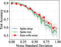
(b) Net Gaussian noise

Figure 3: SVPG: spike/rate coding.

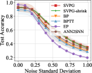
(a) Input Gaussian noise

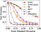
(b) Net Gaussian noise

Figure 4: MNIST: Robustness.

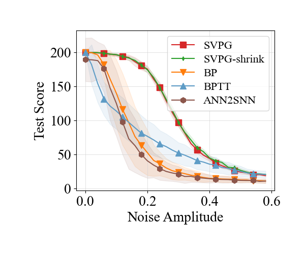
(a) Input uniform noise

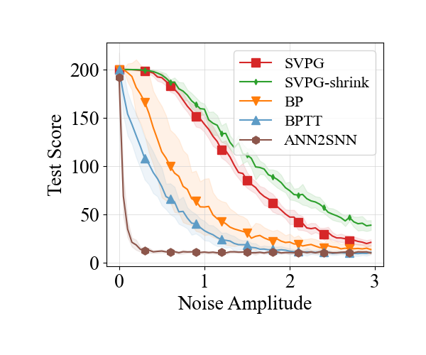
(b) Net uniform noise

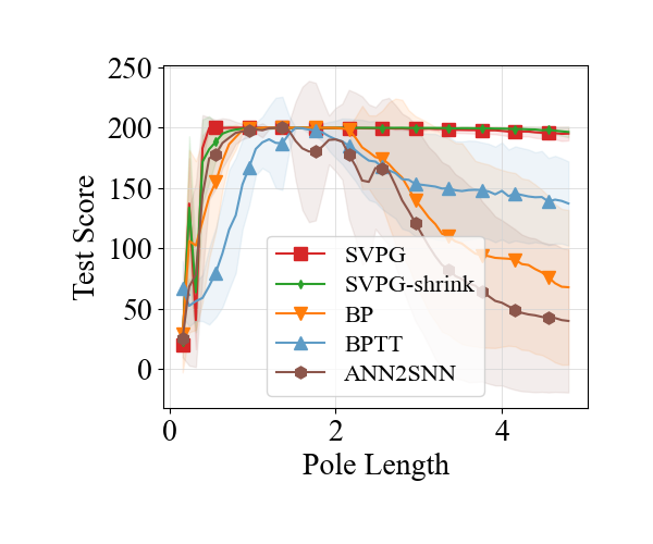
(c) Pendulum length

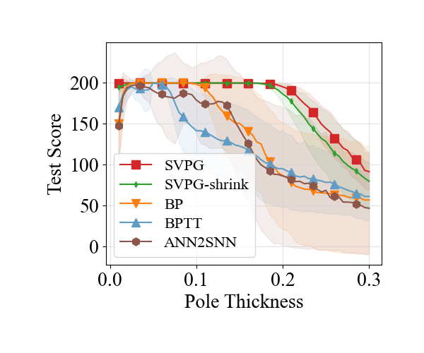
(d) Pendulum thickness

Figure 5: GymIP: Robustness.

   

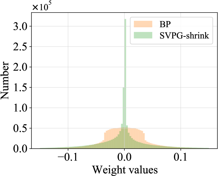
(a) Net weights

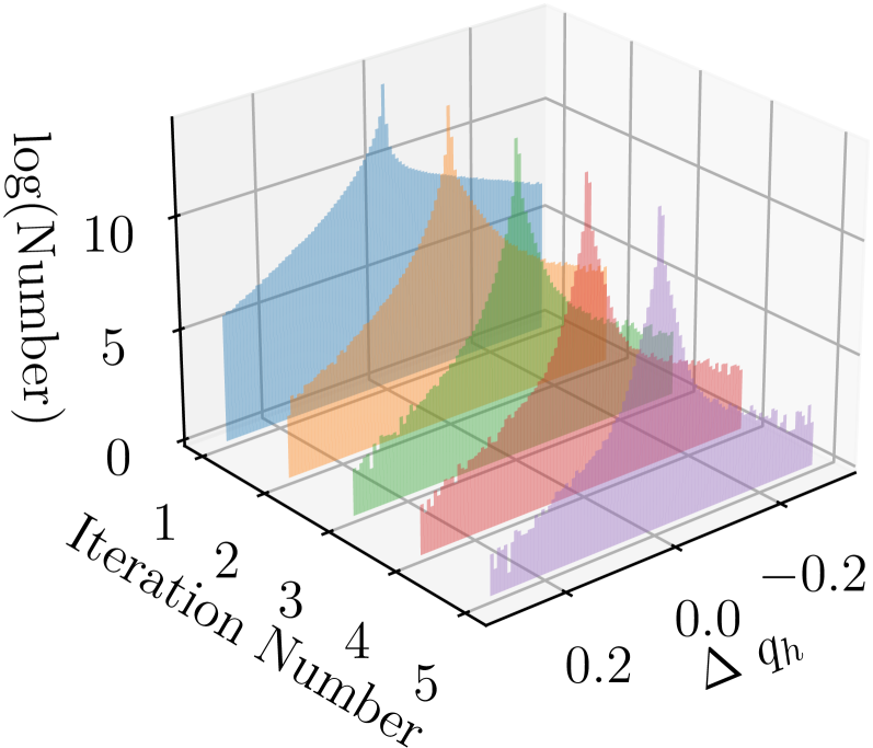
(b) Noise responses

Figure 6:
Visualizations.

SVPG: spike coding versus rate coding

The spike train simulation in SVPG is computationally expensive for common GPUs. With Eq.(7) and Eq.(12), SVPG can also be implemented with rate-coded neuron states, which is more computationally efficient. To reproduce noises caused by spike-train simulation, we add Gaussian noise to rate coding after each iteration of Eq.(7). This results in the “Rate with noise” implementation.

To check whether rate coding alters the performance, we compare it with spike coding in the MNIST task. We consider two different STDP windows – double exponential and rectangle – and name them as “Spike dexp” and “Spike rect”. As in Figure 3 and Appendix D.2, the three implementations generate similar curves, which indicates the rate coding implementation can be used as a replacement for spike coding. In the following experiments, we adopt the rate coding implementation.

4.3 Results

4.3.1 Training Performances

We perform 10 independent training trials (each with a different seed for the random number generator; each with the same number of episodes) for each method. We regularly save checkpoints during training and select the ones with the best zero-noise testing performance as the training results, which are summarized in Table 1. 1) In MNIST, SVPG achieves an accuracy close to BP and outperforms other RL-based methods. Note that although EP achieves high accuracy, it is trained using supervised signals, i.e., does not suffer from the distribution shift in RL. 2) In GymIP, SVPG achieves a near-optimal performance which is close to BP and BPTT. These results indicate that SVPG is able to solve both image-input and long-term decision tasks.

4.3.2 Robustness

We test the learned policies with different kinds of noises. To evaluate the performance, in MNIST, the testing dataset is used; in GymIP, 100 independently sampled episodes are used. We average the results across 10 training trials with different seeds, and present the standard deviations as shaded areas in the figures.

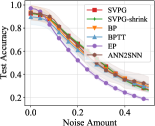
(b) Salt

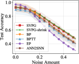
(c) Salt&Pepper

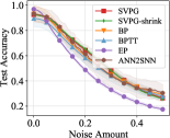
(d) Gaussian&Salt

Figure 9: MNIST – Input noises.

1) Input noise. The results of Gaussian noise in MNIST and uniform noise in GymIP are presented in Figure 4(a), 5(a). Others are in Appendix Figure 9, 11. For all the tested input noises, the performance of SVPG degrades the slowest as the amount/strength of noises increases. For 0.2 uniform noise in the GymIP task, SVPG even achieves more than twice the accuracy of all the compared methods.

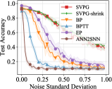
(a) Gaussian

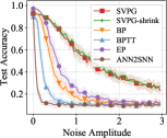
(b) Uniform

Figure 10: MNIST – Network noises.

2) Network parameter noise. The results of Gaussian noise in MNIST and uniform noise in GymIP are in Figure 4(b), 5(b). Other results are in Appendix Figure 10, 12. SVPG achieves slower degradation of performance as the amplitude of noises increases and has a better performance than all compared methods when the strength of noises is large.

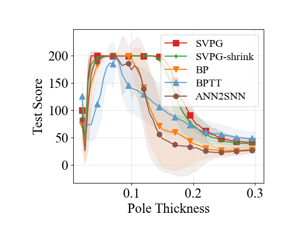
(c) Union

Figure 13: GymIP – Pendulum variations.

3) Environment variations in GymIP. Results on variations in the pendulum’s length and thickness are in Figure 5(c), 5(d). Other variation results are in Appendix Figure 13. When the shape of the pendulum deviates from the one in training, the performance of all the compared methods degrades. However, the performance of SVPG degrades much slower than the baselines. Especially, when changing the pendulum’s length from 1.5 to 4, the performance of SVPG does not appear to degrade. This means the policy trained using SVPG naturally adapts to a larger range of pendulums with different shapes.

The above results show that 1) SVPG can solve classical RL tasks, even with high-dimensional state space. 2) SVPG provides better robustness to the mentioned different kinds of noises and environment variations than the compared methods.

Note that the results about SVPG-shrink and SVPG are similar. These indicate that it is not the larger number of learnable parameters in the RWTA network that brings the above better training performance and robustness.

4.3.3 Additional Results

We check some more properties of SVPG. 1) Network sparsity. We plot the total distribution of synapse weights of 10 training trials (clipped at $\pm 0.15$) in the MNIST task in Figure 6(a). Note that the number of synapse weights in SVPG-shrink and BP are close. As shown, there are more zero weights in SVPG than in BP. This indicates that SVPG tends to learn a more sparse network. 2) Hidden layer response to input noise. Figure 6(b) shows the distribution of changes in the RWTA hidden neurons’ firing probabilities $\Delta q_{h}$ when adding Gaussian noise to input MNIST images (std 0.02), and its relationship with SVPG’s inference iteration number. Results are gained using all 10k testing images and clipped at $\pm 0.3$. In early iterations, the firing probabilities are more affected by the noise as there are more of them that deviate from the no-noise firing probability; in the later iterations, they are less affected. This indicates that the recurrent design of the network should contribute to the robustness of SVPG. 3) Computational costs. We summarize the times needed for inference and optimization stages in Appendix D.5. The rate coding version of SVPG is the fastest in optimization and is only slower than BP in inference.

5 Discussion and Conclusion

This paper proposes SVPG, a spiking-based variational policy gradient method with RWTA network and R-STDP. Current results reveal its potential for solving high-dimensional RL tasks and to have inherent robustness. More theoretical analysis on the cause of robustness, and more experiments in real-world control problems may improve this method and advance the research of biologically plausible methods for RL for applications in real-life scenarios.

Acknowledgements

This work was supported in part by National Natural Science Foundation of China Grant 62206151, China National Postdoctoral Program for Innovative Talents Grant BX20220167, Shuimu Tsinghua Scholar Program, Natural Science Foundation of Fujian Province of China Grant 2022J01656, and UK Royal Society Newton Advanced Fellowship Grant NAF-R1-191082. This work was undertaken in part on ARC3, part of the High Performance Computing facilities at the University of Leeds.

Appendix A Proof of Theorems

A.1 Proof of Theorem 1

Recall that the mean-field inference function is

$$q_{i}={\textstyle\frac{1}{Z(q_{G(i)})}\exp\{\boldsymbol{w}_{{\rm row},i}^{{\rm T}}\boldsymbol{q}+\boldsymbol{w}_{{\rm col},i}^{{\rm T}}\boldsymbol{q}+b_{i}\},}$$ (16)

where $Z(q_{G(i)})={\textstyle\sum_{j\in G(i)}}\exp\{\boldsymbol{w}_{{\rm row},i}^{{\rm T}}\boldsymbol{q}+\boldsymbol{w}_{{\rm col},i}^{{\rm T}}\boldsymbol{q}+b_{i}\}$, $i=1,\dots,(n_{h}d_{h}+d_{a})$, $G(i)$ is the set of indices of the neurons in the same circuit as neuron $i$, and $\boldsymbol{w}_{{\rm row},i}$ and $\boldsymbol{w}_{{\rm col},i}$ are respectively the $i$-th row and column of matrix $\boldsymbol{W}$ (in the shape of a column vector), which corresponds to the synapses connected to neuron $i$. $b_{i}$ is the $i$-th element in vector $\boldsymbol{b}$.

For each $w_{jk}$, There is

$$\frac{\partial q_{i}}{\partial w_{jk}}= -Z^{-2}(q_{G(i)})\frac{\partial Z(q_{G(i)})}{\partial w_{jk}}\exp\left\{\boldsymbol{w}_{{\rm row},i}^{{\rm T}}\boldsymbol{q}+\boldsymbol{w}_{{\rm col},i}^{{\rm T}}\boldsymbol{q}+b_{i}\right\}$$ (17)

$$+Z^{-1}(q_{G(i)})\exp\left\{\boldsymbol{w}_{{\rm row},i}^{{\rm T}}\boldsymbol{q}+\boldsymbol{w}_{{\rm col},i}^{{\rm T}}\boldsymbol{q}+b_{i}\right\}$$

$$\cdot\sum_{m=1}^{N}\left[\frac{\partial(w_{im}+w_{mi})}{\partial w_{jk}}q_{m}+(w_{im}+w_{mi})\frac{\partial q_{m}}{\partial w_{jk}}\right]$$

$$= -q_{i}Z^{-1}(q_{G(i)})\frac{\partial Z(q_{G(i)})}{\partial w_{jk}}+q_{i}\sum_{m=1}^{N}\left[\frac{\partial(w_{im}+w_{mi})}{\partial w_{jk}}q_{m}+(w_{im}+w_{mi})\frac{\partial q_{m}}{\partial w_{jk}}\right].$$

For the term $\frac{\partial Z(q_{G(i)})}{\partial w_{jk}}$, there is

$$\frac{\partial Z(q_{G(i)})}{\partial w_{jk}}= \frac{\partial}{\partial w_{jk}}\left\{\sum_{m\in G(i)}\exp\left\{\boldsymbol{w}_{{\rm row},m}^{{\rm T}}\boldsymbol{q}+\boldsymbol{w}_{{\rm col},m}^{{\rm T}}\boldsymbol{q}+b_{m}\right\}\right\}$$ (18)

$$= \sum_{m\in G(i)}\Big{\{}\exp\big{[}\boldsymbol{w}_{{\rm row},m}^{{\rm T}}\boldsymbol{q}+\boldsymbol{w}_{{\rm col},m}^{{\rm T}}\boldsymbol{q}+b_{m}\big{]}$$

$$\cdot\sum_{n=1}^{N}\big{[}\frac{\partial(w_{mn}+w_{nm})}{\partial w_{jk}}q_{n}+(w_{mn}+w_{nm})\frac{\partial q_{n}}{\partial w_{jk}}\big{]}\Big{\}}.$$

So we have

$$\frac{\partial q_{i}}{\partial w_{jk}}= -q_{i}\sum_{m\in G(i)}\left\{q_{m}\sum_{n=1}^{N}\big{[}\frac{\partial(w_{mn}+w_{nm})}{\partial w_{jk}}q_{n}+(w_{mn}+w_{nm})\frac{\partial q_{n}}{\partial w_{jk}}\big{]}\right\}$$ (19)

$$+q_{i}\sum_{n=1}^{N}\left[\frac{\partial(w_{in}+w_{ni})}{\partial w_{jk}}q_{n}+(w_{in}+w_{ni})\frac{\partial q_{n}}{\partial w_{jk}}\right].$$

Similarly, for each $b_{j}$, there is

$$\frac{\partial q_{i}}{\partial b_{j}}=-q_{i}\sum_{m\in G(i)}\left\{q_{m}\left[\frac{\partial b_{m}}{\partial b_{j}}+\sum_{n=1}^{N}(w_{mn}+w_{nm})\frac{\partial q_{n}}{\partial_{b_{j}}}\right]\right\}+q_{i}\left[\frac{\partial b_{i}}{\partial b_{j}}+\sum_{n=1}^{N}(w_{in}+w_{ni})\frac{\partial q_{n}}{\partial_{b_{j}}}\right].$$ (20)

By respectively arranging Eq. (19) and Eq. (20) for each $q_{i}$ into vectors, and combining the terms into matrices, we can get the Eq. (10) in Theorem 1. $\square$

A.2 Proof of Theorem 2

The condition is the same as that in the proof of Theorem 1. The approximate differentiation of firing rate $q_{i}$ with respect to $w_{jk}$ and $b_{j}$ are:

$$\frac{\partial\log(q_{i})}{\partial w_{jk}}= \sum_{m=1}^{N}\Big{[}\frac{\partial(w_{im}+w_{mi})}{\partial w_{jk}}q_{m}\Big{]}$$ (21)

$$-\frac{1}{Z(q_{G(i)})}\sum_{m\in G(i)}\Big{[}\exp\{\boldsymbol{w}_{{\rm row},m}^{{\rm T}}\boldsymbol{q}+\boldsymbol{w}_{{\rm col},m}^{{\rm T}}\boldsymbol{q}+b_{m}\}\cdot\sum_{n=1}^{N}\frac{\partial(w_{mn}+w_{nm})}{\partial w_{jk}}q_{n}\Big{]}$$

$$= \sum_{m=1}^{N}\Big{[}\frac{\partial(w_{im}+w_{mi})}{\partial w_{jk}}q_{m}\Big{]}-\sum_{m\in G(i)}\Big{[}q_{m}\cdot\sum_{n=1}^{N}\frac{\partial(w_{mn}+w_{nm})}{\partial w_{jk}}q_{n}\Big{]},$$

$$\frac{\partial\log(q_{i})}{\partial b_{j}}= \frac{\partial b_{i}}{\partial b_{j}}-\frac{1}{Z(q_{G(i)})}\cdot\sum_{m\in G(i)}\Big{[}\frac{\partial b_{m}}{\partial b_{j}}\cdot\exp\{\boldsymbol{w}_{{\rm row},m}^{{\rm T}}\boldsymbol{q}+\boldsymbol{w}_{{\rm col},m}^{{\rm T}}\boldsymbol{q}+b_{m}\}\Big{]}$$ (22)

$$= \frac{\partial b_{i}}{\partial b_{j}}-\sum_{m\in G(i)}\Big{[}q_{m}\frac{\partial b_{m}}{\partial b_{j}}\Big{]}.$$

Similar to the proof of Theorem 1, by respectively arranging Eq. (21) and Eq. (22) for each $q_{i}$ into vectors, and combining the terms on the right hand side into matrices, we can get the Eq. (11) in Theorem 2. $\square$

Appendix B SVPG Algorithm Details

We summarize the overall working flow with our RWTA network as Algorithm 1. For conciseness, this algorithm does not cover the implementation of spike-based inference and STDP-based optimization. Note that these spike-related implementations can be done by simply replacing Eq.(7) with Eq.(9), and applying Eq.(13).

In practice, Actor-Critic (AC) based methods are more commonly used than vanilla Policy Gradient (PG). The main difference between AC and PG is that AC learns an extra value function in the place of $r_{t}$ in PG. To adapt our algorithm to AC, we add a multi-layer perceptron trained with backpropagation to estimate the critic value function, and use the estimated value to replace the $r_{t}$ in Eq.(1).

The SVPG implemented with REINFORCE algorithm is presented in Algorithm 1. The equation numbers correspond to the equations in the main text.

Algorithm 1 SVPG with REINFORCE

Input: Discount factor $\gamma$. Training episode number $N_{\rm epi}$. Inference iteration number $N_{\rm iter}$. Learning rate $\eta$.
Parameter: Network shape $n_{h},d_{h},d_{a},d_{s}$.
Output: RWTA Network parameter $\theta$.

1:  Initialize $\theta$.

2:  for Episode = 1, …, $N_{\rm epi}$ do

3:     Clear memory buffer $\mathcal{D}$.

4:     for Training step t = 1, …, $T$ do

5:        Observe and encode state $s_{t}$.

6:        Random initialize $\boldsymbol{q}_{a}$ and $\boldsymbol{q}_{h}$.

7:        Iterate Eq.(7) until convergence. {Inference}

8:        Sample action $a_{t}$ using $\boldsymbol{q}_{a}$.

9:        Perform $a_{t}$, observe reward $r_{t}$ and new state $s_{t+1}$.

10:        Store $\langle s_{t},a_{t},r_{t},s_{t+1},\boldsymbol{q},\boldsymbol{v}\rangle$ into $\mathcal{D}$.

11:     end for

12:     Get data from $\mathcal{D}$.

13:     Calculate gradient using Eq.(1), Eq.(12), Eq.(11). {Optimize}

14:     Update $\theta\leftarrow\theta+\eta\nabla\theta$

15:  end for

Appendix C Experiment Details

C.1 Task Details

MNIST task. In this task, each episode includes only one time step. At the time step, the agent observes a randomly selected image from the MNIST training dataset, and selects one of the ten categories as its action. The input images are of size $28\times 28$ and are in grayscale. The range of values is converted to $[0,1]$ by dividing $255$. For all the algorithms compared, the input images are stretched to vectors (with length $784$). A reward of $+1$ indicates a correct selection, $-1$ the opposite. The maximum length of training is set to 50k steps (in each step a randomly selected 100-size batch is used for training) so that in practice all the methods converge. During training, a checkpoint of the network parameters is saved every 100 training steps. After training, the checkpoint with the best accuracy in the testing set (without noise) is reloaded to do the testing. The MNIST testing dataset is used in testing.

GymIP task. Each episode has a maximum of $200$ time steps, with a reward of $+1$ for each step. The episodes end early if the pendulum (pole) falls. The observation is a $4$-dimensional vector with no predefined ranges. To normalize the observations to the range of $[0,1]$, we use a random policy to sample from the environment, and use the samples’ range to determine a linear mapping to the range of $[0,1]$. In our experiments, the sampled ranges are $[-0.4,0.4]$, $[-0.2,0.2]$, $[-1.7,1.7]$, $[-1.25,1.25]$. The action space consists of 5 discrete actions, evenly extracted from the range $[-3,3]$. The maximum length of training is set to 20k episodes. During training, a checkpoint of the network parameters is saved every 20 episodes. After training, the checkpoint with the best performance is reloaded to do the testing.

C.2 Implementation Details

Network Sizes. 1) For the MNIST task, SVPG uses an RWTA network with 784 input neurons, 20 hidden WTA circuits each with 10 neurons, and 10 output neurons; SVPG-shrink uses a smaller RWTA network where the number of hidden WTA circuits is changed to 17 so that the total number of learnable parameters is close to other methods; BP, BPTT, ANN2SNN, and EP use layered networks with 784 input neurons, 1 hidden layer with 200 neurons, and 10 output neurons. 2) For the GymIP task, SVPG uses an RWTA network with 4 input neurons, 8 hidden WTA circuits each with 8 neurons, and 5 output neurons; SVPG-shrink uses a smaller RWTA network where the number of hidden WTA circuits is changed to 3. BP, BPTT, and ANN2SNN use layered networks with 4 input neurons, 1 hidden layer with 64 hidden neurons, and 5 output neurons. 3) For the GymIP task there is a critic network used in all the methods. This critic network is layered, with 4 input neurons, 2 hidden layers each with 64 neurons, and 5 output neurons.

Optimizer. For the compared methods, i.e., BP, BPTT, and EP, we select the stochastic gradient descent (SGD) with zero momentum for the MNIST task, and select the RMSprop optimizer for the GymIP task. For the SGD optimizer, we incompletely tried learning rates ranging from 0.001 to 0.3, and found 0.1 to be a good balance between training speed and stability. For the RMSprop optimizer, we use a learning rate of 0.001. As for SVPG, we use a learning rate of 0.1 in the MNIST task and 0.001 in the GymIP task.

RL hyper-parameters. The GymIP task involves sequential decisions which may have long-term effects on rewards. We select the discount rate $\gamma$ to be 0.999 (close to 1) so that the discounted sum of rewards reflects the length of the episodes, maximizing which is the task objective. To stabilize training, we use a replay buffer with a size of 100. To encourage the agent to explore more actions, we add an intrinsic exploration reward to the environment reward; the reward is calculated as the entropy of the agent’s action distribution; the ratio of the environment reward and the intrinsic reward is 2:1.

Appendix D Additional Experiment Results

D.1 MNIST Input Noise Illustration

0    0.2 0.4 0.6 0.8 1.0    

Figure 7: Some input images with different strengths of Gaussian noises in MNIST task. Standard deviation noted above images.

D.2 Additional Comparison of Three SVPG Implementations

In the main text, we present the results regarding input salt noise and network Gaussian noise. Here we present the results with other noises, as shown in Figure 8. These results further support the analysis in the main text.

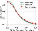
(a) Input Gaussian

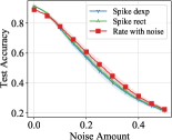
(b) Input Gaussian&Salt

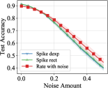
(c) Input Salt&Pepper

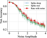
(d) Network Uniform

Figure 8: Additional comparison of three implementations of SVPG.

D.3 MNIST Additional Results

(a) Gaussian

D.4 GymIP Additional Results

Here are the complete results of all the variations tested in the GymIP task. Note that the “Union” variation means the length and thickness of the pendulum change together with a fixed ratio (length:thickness=16:1).

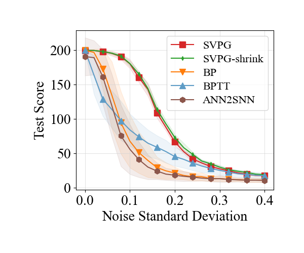
(a) Gaussian

(b) Uniform

Figure 11: GymIP – Input noises.

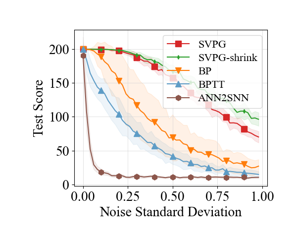
(a) Gaussian

(b) Uniform

Figure 12: GymIP – Network noises.

(a) Length

(b) Thickness

D.5 Computation Costs

The computation costs of inference and optimization of different methods in the MNIST task are shown in Table 2. The values presented are the averaged times of 10 steps. The results are gained using one NVIDIA RTX 3080 GPU. 1) For the inference period, SVPG consumes much more time than BP and EP. This is because SVPG needs to simulate a spike train during each inference step. The rate coding version of SVPG alleviates this problem and achieves a computational efficiency close to that of BP and EP. 2) For the optimization period, SVPG is the most efficient. This is because SVPG updates the parameters using only local learning rules, while other methods need backpropagation (BP and BPTT) or iterations (EP).

Time (ms)	SVPG-rate	SVPG-spike	BP	BPTT	EP
Inference	2.1	373.1	0.2	52.5	4.3
Optimization	0.2	0.5	1.6	60.1	61.1

Table 2: Computation costs.

References

- [Asgari et al.(2020)Asgari, Maybodi, Payvand, et al.] Hajar Asgari, Babak Mazloom-Nezhad Maybodi, Melika Payvand, et al. Low-Energy and Fast Spiking Neural Network for Context-Dependent Learning on FPGA. IEEE Transactions on Circuits and Systems II: Express Briefs, 67(11):2697–2701, 2020.
- [Beck et al.(2012)Beck, Heller, and Pouget] Jeffrey M. Beck, Katherine A. Heller, and Alexandre Pouget. Complex Inference in Neural Circuits with Probabilistic Population Codes and Topic Models. In NeurIPS, pages 3068–3076, 2012.
- [Bellec et al.(2020)Bellec, Scherr, Subramoney, et al.] Guillaume Bellec, Franz Scherr, Anand Subramoney, et al. A Solution to the Learning Dilemma for Recurrent Networks of Spiking Neurons. Nature Communications, 11(1):3625, 2020.
- [Bellemare et al.(2020)Bellemare, Candido, Castro, et al.] Marc G. Bellemare, Salvatore Candido, Pablo Samuel Castro, et al. Autonomous Navigation of Stratospheric Balloons Using Reinforcement Learning. Nature, 588(7836):77–82, 2020.
- [Bing et al.(2019)Bing, Jiang, Cheng, et al.] Zhenshan Bing, Zhuangyi Jiang, Long Cheng, et al. End to End Learning of a Multi-Layered SNN based on R-STDP for a Target Tracking Snake-like Robot. In ICRA, pages 9645–9651, 2019.
- [Chung and Kozma(2020)] Stephen Chung and Robert Kozma. Reinforcement Learning with Feedback-Modulated TD-STDP. arXiv:2008.13044 [cs, stat], 2020.
- [Devo et al.(2020)Devo, Mezzetti, Costante, et al.] A. Devo, G. Mezzetti, G. Costante, et al. Towards Generalization in Target-Driven Visual Navigation by Using Deep Reinforcement Learning. IEEE Transactions on Robotics, 36(5):1546–1561, 2020.
- [Frémaux and Gerstner(2016)] Nicolas Frémaux and Wulfram Gerstner. Neuromodulated Spike-Timing-Dependent Plasticity, and Theory of Three-Factor Learning Rules. Frontiers in Neural Circuits, 9, 2016.
- [Gallego et al.(2022)Gallego, Delbruck, Orchard, Bartolozzi, Taba, Censi, Leutenegger, Davison, Conradt, Daniilidis, and Scaramuzza] Guillermo Gallego, Tobi Delbruck, Garrick Orchard, Chiara Bartolozzi, Brian Taba, Andrea Censi, Stefan Leutenegger, Andrew Davison, Jorg Conradt, Kostas Daniilidis, and Davide Scaramuzza. Event-based vision: A survey. IEEE Transactions on Pattern Analysis and Machine Intelligence, 44(1):154–180, 2022.
- [Gerstner et al.(2014)Gerstner, Kistler, Naud, et al.] Wulfram Gerstner, Werner M. Kistler, Richard Naud, et al. Neuronal Dynamics: From Single Neurons to Networks and Models of Cognition. Cambridge University Press, 2014. ISBN 978-1-107-44761-5.
- [Guo et al.(2019)Guo, Yu, Deng, et al.] Shangqi Guo, Zhaofei Yu, Fei Deng, et al. Hierarchical Bayesian Inference and Learning in Spiking Neural Networks. IEEE Transactions on Cybernetics, 49(1):133–145, 2019.
- [Heess et al.(2013)Heess, Silver, and Teh] Nicolas Heess, David Silver, and Yee Whye Teh. Actor-Critic Reinforcement Learning with Energy-Based Policies. In Proceedings of the Tenth European Workshop on Reinforcement Learning, pages 45–58, 2013.
- [Jang et al.(2020)Jang, Skatchkovsky, and Simeone] Hyeryung Jang, Nicolas Skatchkovsky, and Osvaldo Simeone. VOWEL: A Local Online Learning Rule for Recurrent Networks of Probabilistic Spiking Winner- Take-All Circuits. In ICPR 2020, pages 4597–4604, 2020.
- [Kappel et al.(2018)Kappel, Legenstein, Habenschuss, et al.] David Kappel, Robert Legenstein, Stefan Habenschuss, et al. A Dynamic Connectome Supports the Emergence of Stable Computational Function of Neural Circuits through Reward-Based Learning. eNeuro, 5(2):ENEURO–0301, 2018.
- [LeCun et al.(2015)LeCun, Bengio, and Hinton] Yann LeCun, Yoshua Bengio, and Geoffrey Hinton. Deep learning. Nature, 521(7553):436–444, May 2015. ISSN 1476-4687.
- [Li et al.(2020)Li, Chen, Moutafis, et al.] Chen Li, Runze Chen, Christoforos Moutafis, et al. Robustness to Noisy Synaptic Weights in Spiking Neural Networks. In IJCNN, 2020.
- [Lillicrap et al.(2016)Lillicrap, Hunt, Pritzel, et al.] Timothy P. Lillicrap, Jonathan J. Hunt, Alexander Pritzel, et al. Continuous Control with Deep Reinforcement Learning. In ICLR, 2016.
- [Lovatto et al.(2019)Lovatto, Bueno, and de Barros] Ângelo Gregório Lovatto, Thiago Pereira Bueno, and Leliane Nunes de Barros. Analyzing the Effect of Stochastic Transitions in Policy Gradients in Deep Reinforcement Learning. In BRACIS, pages 413–418, 2019.
- [Manrique Escobar et al.(2020)Manrique Escobar, Pappalardo, and Guida] Camilo Andrés Manrique Escobar, Carmine Maria Pappalardo, and Domenico Guida. A Parametric Study of a Deep Reinforcement Learning Control System Applied to the Swing-Up Problem of the Cart-Pole. Applied Sciences, 10(24), 2020.
- [Mnih et al.(2016)Mnih, Badia, Mirza, et al.] Volodymyr Mnih, Adria Puigdomenech Badia, Mehdi Mirza, et al. Asynchronous Methods for Deep Reinforcement Learning. In ICML, pages 1928–1937, 2016.
- [Özalp et al.(2020)Özalp, Varol, Taşci, and Uçar] Recep Özalp, Nuri Köksal Varol, Burak Taşci, and Ayşegül Uçar. A Review of Deep Reinforcement Learning Algorithms and Comparative Results on Inverted Pendulum System, pages 237–256. Springer International Publishing, 2020.
- [Patel et al.(2019)Patel, Hazan, Saunders, et al.] Devdhar Patel, Hananel Hazan, Daniel J Saunders, et al. Improved Robustness of Reinforcement Learning Policies upon Conversion to Spiking Neuronal Network Platforms Applied to Atari Breakout Game. Neural Networks, 120:108–115, 2019.
- [Rezende et al.(2011)Rezende, Wierstra, and Gerstner] Danilo Rezende, Daan Wierstra, and Wulfram Gerstner. Variational Learning for Recurrent Spiking Networks. In NeurIPS, 2011.
- [Rueckauer et al.(2017)Rueckauer, Lungu, Hu, et al.] Bodo Rueckauer, Iulia-Alexandra Lungu, Yuhuang Hu, et al. Conversion of Continuous-Valued Deep Networks to Efficient Event-Driven Networks for Image Classification. Frontiers in Neuroscience, 11:682, 2017.
- [Scellier and Bengio(2017)] Benjamin Scellier and Yoshua Bengio. Equilibrium Propagation: Bridging the Gap between Energy-Based Models and Backpropagation. Frontiers in Computational Neuroscience, 11:24, 2017.
- [Schulman et al.(2017)Schulman, Wolski, Dhariwal, et al.] John Schulman, Filip Wolski, Prafulla Dhariwal, et al. Proximal Policy Optimization Algorithms. CoRR, abs/1707.06347, 2017.
- [Sharmin et al.(2019)Sharmin, Panda, Sarwar, Lee, Ponghiran, and Roy] Saima Sharmin, Priyadarshini Panda, Syed Shakib Sarwar, Chankyu Lee, Wachirawit Ponghiran, and Kaushik Roy. A Comprehensive Analysis on Adversarial Robustness of Spiking Neural Networks. In IJCNN, 2019.
- [Suhaimi et al.(2022)Suhaimi, Lim, Chia, Li, and Makino] Ahmad Suhaimi, Amos Lim, Xin Chia, Chunyue Li, and Hiroshi Makino. Representation learning in the artificial and biological neural networks underlying sensorimotor integration. Science Advances, 8(22), 2022.
- [Sutton and Barto(2018)] Richard S. Sutton and Andrew G. Barto. Reinforcement Learning: An Introduction. MIT press, 2018.
- [Wainwright and Jordan(2008)] Martin J. Wainwright and Michael I. Jordan. Graphical Models, Exponential Families, and Variational Inference. Foundations & Trends in Machine Learning, 1(1-2):1–305, 2008.
- [Wunderlich et al.(2019)Wunderlich, Kungl, Müller, et al.] Timo Wunderlich, Akos F Kungl, Eric Müller, et al. Demonstrating Advantages of Neuromorphic Computation: A Pilot Study. Frontiers in Neuroscience, 13:260, 2019.
- [Yanguas-Gil(2020)] Angel Yanguas-Gil. Coarse Scale Representation of Spiking Neural Networks: Backpropagation through Spikes and Application to Neuromorphic Hardware. In ICNS, 2020.
- [Yu et al.(2018)Yu, Deng, Guo, Yan, Liu, and Chen] Zhaofei Yu, Fei Deng, Shangqi Guo, Qi Yan, Jian K. Liu, and Feng Chen. Emergent Inference of Hidden Markov Models in Spiking Winner-Take-All Neural Networks. IEEE Transactions on Cybernetics, 2018.
- [Yu et al.(2020)Yu, Liu, Jia, Zhang, Zheng, Tian, and Huang] Zhaofei Yu, Jian K. Liu, Shanshan Jia, Yichen Zhang, Yajing Zheng, Yonghong Tian, and Tiejun Huang. Toward the Next Generation of Retinal Neuroprosthesis: Visual Computation with Spikes. Engineering, 6(4):449–461, 2020.
- [Yuan et al.(2019)Yuan, Wu, Yan, et al.] Mengwen Yuan, Xi Wu, Rui Yan, et al. Reinforcement Learning in Spiking Neural Networks with Stochastic and Deterministic Synapses. Neural Computation, 31(12):2368–2389, 2019.
- [Zenke and Ganguli(2018)] Friedemann Zenke and Surya Ganguli. SuperSpike: Supervised Learning in Multilayer Spiking Neural Networks. Neural Computation, 30(6), 2018.