Positive Einstein metrics with $\mathbb{S}^{4m+3}$ as principal orbit

Abstract

We prove that there exists at least one positive Einstein metric on $\mathbb{HP}^{m+1}\sharp\overline{\mathbb{HP}}^{m+1}$ for $m\geq 2$. Based on the existence of the first Einstein metric, we give a criterion to check the existence of a second Einstein metric on $\mathbb{HP}^{m+1}\sharp\overline{\mathbb{HP}}^{m+1}$. We also investigate the existence of cohomogeneity one positive Einstein metrics on $\mathbb{S}^{4m+4}$ and prove the existence of a non-standard Einstein metric on $\mathbb{S}^{8}$.

1 Introduction

A Riemannian manifold $(M,g)$ is Einstein if its Ricci curvature is a constant multiple of $g$:

$$\mathrm{Ric}(g)=\Lambda g.$$

The metric $g$ is then called an Einstein metric and $\Lambda$ is the Einstein constant. Depending on the sign of $\Lambda$, we call $g$ a positive Einstein ($\Lambda>0$) metric, a negative Einstein ($\Lambda<0$) metric or a Ricci-flat ($\Lambda=0$) metric. A positive Einstein manifold is compact by Myers’ Theorem [Mye41].

In this article, we investigate the existence of positive Einstein metrics of cohomogeneity one. A Riemannian manifold $(M,g)$ is of cohomogeneity one if a Lie Group $\mathsf{G}$ acts isometrically on $M$ such that the principal orbit $\mathsf{G}/\mathsf{K}$ is of codimension one. The first example of an inhomogeneous positive Einstein metric was constructed in [Pag78]. The metric is defined on $\mathbb{CP}^{2}\sharp\overline{\mathbb{CP}}^{2}$ and is of cohomogeneity one. The result was later generalized in [BB82], [KS86], [Sak86], [PP87], [KS88] and [WW98]. A common feature shared by positive Einstein metrics constructed in this series of works is the principal orbits being principal $U(1)$-bundles over either a Fano manifold or a product of Fano manifolds. From this perspective, one can view the Einstein metric on $\mathbb{HP}^{2}\sharp\overline{\mathbb{HP}}^{2}$ in [Böh98] as another type of generalization to the Page’s metric, whose principal orbit is a principal $Sp(1)$-bundle over $\mathbb{HP}^{1}$.

A natural question arises whether there exists a positive Einstein metric of cohomogeneity one on $\mathbb{HP}^{m+1}\sharp\overline{\mathbb{HP}}^{m+1}$ with $m\geq 2$, where the principal orbit is the total space of the quaternionic Hopf fibration formed by the following group triple:

$$(\mathsf{K},\mathsf{H},\mathsf{G})=(Sp(m)\Delta Sp(1),Sp(m)Sp(1)Sp(1),Sp(m+1)Sp(1)).$$ (1.1)

The condition of being $\mathsf{G}$-invariant reduces the Einstein equations to an ODE system defined on the 1-dimensional orbit space. The solution takes the form of $g=dt^{2}+g(t),$ where $g(t)$ is a $\mathsf{G}$-invariant metric on $\mathbb{S}^{4m+3}$ for each $t$. One looks for a $g(t)$ that is defined on a closed interval $[0,T]$ with an initial condition and a terminal condition. If $g(t)$ collapses to the quaternionic-Kähler metric on the singular orbit $\mathbb{HP}^{m}$ at $t=0$ and $t=T$, then $g$ defines a positive Einstein metric on the connected sum $\mathbb{HP}^{m+1}\sharp\overline{\mathbb{HP}}^{m+1}$, or equivalently, an $\mathbb{S}^{4}$-bundle over $\mathbb{HP}^{m}$. It has been conjectured that such an Einstein metric exists on $\mathbb{HP}^{m+1}\sharp\overline{\mathbb{HP}}^{m+1}$ for all $m\geq 2$, as indicated by numerical evidence provided in [PP86], [Böh98] and [DHW13].

Some well-known Einstein metrics are realized as integral curves to the cohomogeneity one Einstein equation. For example, the standard sphere metric, the sine cone over Jensen’s sphere, and the quaternionic-Kähler metric on $\mathbb{HP}^{m+1}$ are represented by integral curves to the cohomogeneity one system. Furthermore, the cone solution is an attractor to the system. It was realized in [Böh98] that the winding of integral curves around the cone solution plays an important role in the existence problem described above. To investigate the winding, one studies a quantity (denoted as $\sharp C_{w}(\bar{h})$ in [Böh98]) that is assigned to each local solution that does not globally define a complete Einstein metric on $\mathbb{HP}^{m+1}\sharp\overline{\mathbb{HP}}^{m+1}$. From the point of view of geometry, the quantity records the number of times that the principal orbit becomes isoparametric while its mean curvature remains positive. In general, an estimate for $\sharp C_{w}(\bar{h})$ can be obtained from the linearization along the cone solution. For $m=1$, the estimate is good enough to prove the global existence. This is not the case, however, if $m\geq 2$. For higher dimensional cases, it is from the global analysis of the system that we obtain a further estimate for $\sharp C_{w}(\bar{h})$ and we prove the following existence theorem.

Theorem 1.1.

On each $\mathbb{HP}^{m+1}\sharp\overline{\mathbb{HP}}^{m+1}$ with $m\geq 2$, there exists at least one positive Einstein metric with $\mathsf{G}/\mathsf{K}=\mathbb{S}^{4m+3}$ as its principal orbit.

Numerical studies in [Böh98] and [DHW13] indicate that there exists another Einstein metric on $\mathbb{HP}^{m+1}\sharp\overline{\mathbb{HP}}^{m+1}$ with $m\geq 2$. Based on Theorem 1.1, an estimate for $\sharp C_{w}(\bar{h})$ in a limiting subsystem (essentially obtained from the linearization along the cone solution) helps us propose a criterion to check the existence of the second Einstein metric. Let $n$ be the dimension of $\mathsf{G}/\mathsf{K}$. Such a criterion only depends on $n$ (or $m$).

Theorem 1.2.

Let $\theta_{\Psi}$ be the solution to the following initial value problem:

$$\frac{d\theta}{d\eta}=\frac{n-1}{2n}\tanh\left(\frac{2\eta}{n}\right)\sin(2\theta)+\frac{2}{n}\sqrt{\frac{(2m+1)(2m+2)(2m+3)}{(2m+3)^{2}+2m}},\quad\theta(0)=0.$$ (1.2)

Let $\Omega=\lim\limits_{\eta\to\infty}\theta_{\Psi}$. For $m\geq 2$, there exist at least two positive Einstein metrics on $\mathbb{HP}^{m+1}\sharp\overline{\mathbb{HP}}^{m+1}$ if $\Omega<\frac{3\pi}{4}$.

The upper bound for $\Omega$ in Theorem 1.2 is not sharp. Although it is difficult to solve the initial value problem (1.2) explicitly, one can use the Runge–Kutta 4-th order algorithm to approximate $\Omega$. Since the RHS of (1.2) does not vanish at $\eta=0$, the initial Runge–Kutta step is well-defined. Our numerical study shows that $\Omega<\frac{3\pi}{4}$ for integers $m\in[2,100]$.

We also look into the case where $\mathsf{G}/\mathsf{K}$ completely collapses at two ends of a compact manifold. In that case, the cohomogeneity one space is $\mathbb{S}^{4m+4}$. No new Einstein metric is found on $\mathbb{S}^{4m+4}$ for $m\geq 2$. For $m=1$, however, we obtained a non-standard positive Einstein metric on $\mathbb{S}^{8}$. Such a metric is inhomogeneous by the classification in [Zil82].

Theorem 1.3.

There exists a non-standard $Sp(2)Sp(1)$-invariant positive Einstein metric $\hat{g}_{\mathbb{S}^{8}}$ on $\mathbb{S}^{8}$.

It is worth mentioning that all new solutions found are symmetric. Metrics that are represented by these solutions all have a totally geodesic principal orbit.

This article is structured as follows. In Section 2, we present the dynamical system for positive Einstein metrics of cohomogeneity one with $\mathsf{G}/\mathsf{K}$ as the principal orbit. Then we apply a coordinate change that makes the cohomogeneity one Ricci-flat system serve as a limiting subsystem. Initial conditions and terminal conditions are transformed into critical points of the new system. The new system admits $\mathbb{Z}_{2}$-symmetry. By a sign change, one can transform initial conditions into terminal conditions. Hence the problem of finding globally defined positive Einstein metrics boils down to finding heteroclines that join two different critical points.

In Section 3, we compute linearizations of the critical points mentioned above and obtain two 1-parameter families of locally defined positive Einstein metrics. One family is defined on a tubular neighborhood around $\mathbb{HP}^{m}$, represented by a 1-parameter family of integral curves $\gamma_{s_{1}}$. The other family is defined on a neighborhood of a point in $\mathbb{S}^{4m+4}$, represented by another 1-parameter family of integral curves $\zeta_{s_{2}}$.

In Section 4, we make a little modification on the quantity $\sharp C_{w}(\bar{h})$ in [Böh98] and it is assigned to both $\gamma_{s_{1}}$ and $\zeta_{s_{2}}$ (hence denoted as $\sharp C(\gamma_{s_{1}})$ and $\sharp C({\zeta_{s_{2}}})$). We construct a compact set to obtain an estimate for $\sharp C(\gamma_{s_{1}})$ of some local solutions. Then we apply Lemma 4.4 in [Böh98] and prove Theorem 1.1.

In Section 5, we apply another coordinate change that allows us to obtain more information on $\sharp C(\gamma_{s_{1}})$ and $\sharp C(\zeta_{s_{2}})$, which is encoded in the initial value problem (1.2) in Theorem 1.2. We also prove Theorem 1.3.

Visual summaries of Theorem 1.1-1.3 are presented at the end of this article.

Acknowledgments The research is funded by NSFC (No. 12071489), the Foundation for Young Scholars of Jiangsu Province, China (BK-20220282), and XJTLU Research Development Funding (RDF-21-02-083). The author is grateful to McKenzie Wang for his constant support and encouragement. The author would like to thank Christoph Böhm for his helpful suggestions and remarks on this project. The author also thanks Cheng Yang and Wei Yuan for many inspiring discussions.

2 Cohomogeneity one system

Consider the group triple $(\mathsf{K},\mathsf{H},\mathsf{G})$ in (1.1). The isotropy representation $\mathfrak{g}/\mathfrak{k}$ consists of two inequivalent irreducible summands $\mathfrak{p}_{1}=\mathfrak{h}/\mathfrak{k}$ and $\mathfrak{p}_{2}=\mathfrak{g}/\mathfrak{h}$. Let the standard sphere metric $g_{\mathbb{S}^{4m+3}}$ on $\mathsf{G}/\mathsf{K}=\mathbb{S}^{4m+3}$ be the background metric. As any $\mathsf{G}$-invariant metric on $\mathsf{G}/\mathsf{K}$ is determined by its restriction to one tangent space $\mathfrak{g}/\mathfrak{k}$, the metric has the form of

$$f_{1}^{2}\left.g_{\mathbb{S}^{4m+3}}\right|_{\mathfrak{p}_{1}}+f_{2}^{2}\left.g_{\mathbb{S}^{4m+3}}\right|_{\mathfrak{p}_{2}}.$$

Let $f_{1}$ and $f_{2}$ be functions that are defined on the 1-dimensional orbit space. We consider Einstein equations for the cohomogeneity one metric

$$g:=dt^{2}+f_{1}^{2}\left.g_{\mathbb{S}^{4m+3}}\right|_{\mathfrak{p}_{1}}+f_{2}^{2}\left.g_{\mathbb{S}^{4m+3}}\right|_{\mathfrak{p}_{2}}.$$

By [EW00], the metric $g$ is an Einstein metric on $(t_{*}-\epsilon,t_{*}+\epsilon)\times\mathsf{G}/\mathsf{K}$ if $(f_{1},f_{2})$ is a solution to

$$\begin{split}&\frac{\ddot{f_{1}}}{f_{1}}-\left(\frac{\dot{f_{1}}}{f_{1}}\right)^{2}=-\left(3\frac{\dot{f_{1}}}{f_{1}}+4m\frac{\dot{f_{2}}}{f_{2}}\right)\frac{\dot{f_{1}}}{f_{1}}+2\frac{1}{f_{1}^{2}}+4m\frac{f_{1}^{2}}{f_{2}^{4}}-\Lambda,\\ &\frac{\ddot{f_{2}}}{f_{2}}-\left(\frac{\dot{f_{2}}}{f_{2}}\right)^{2}=-\left(3\frac{\dot{f_{1}}}{f_{1}}+4m\frac{\dot{f_{2}}}{f_{2}}\right)\frac{\dot{f_{2}}}{f_{2}}+(4m+8)\frac{1}{f_{2}^{2}}-6\frac{f_{1}^{2}}{f_{2}^{4}}-\Lambda,\end{split}$$ (2.1)

with a conservation law

$$3\left(\frac{\dot{f_{1}}}{f_{1}}\right)^{2}+4m\left(\frac{\dot{f_{2}}}{f_{2}}\right)^{2}-\left(d_{1}\frac{\dot{f_{1}}}{f_{1}}+d_{2}\frac{\dot{f_{2}}}{f_{2}}\right)^{2}+6\frac{1}{f_{1}^{2}}+4m(4m+8)\frac{1}{f_{2}^{2}}-12m\frac{f_{1}^{2}}{f_{2}^{4}}-(n-1)\Lambda=0.$$ (2.2)

To fix homothety, we set $\Lambda=n$ in this article. We leave $\Lambda$ in the equations for readers to trace the Einstein constant.

Remark 2.1.

If we replace the principal orbit $\mathsf{G}/\mathsf{K}$ by $\mathbb{S}^{4m+3}=[Sp(m+1)U(1)]/[Sp(m)\Delta U(1)]$, then the isotropy representation $\mathfrak{g}/\mathfrak{k}$ consists of three inequivalent irreducible summands. The principal orbit can collapse either as $\mathbb{HP}^{m}$ or $\mathbb{CP}^{2m+1}$, depending on the choice of intermediate group. For such a principal orbit, the dynamical system of cohomogeneity one Einstein metrics involves three functions and has (2.1) as its subsystem. A numerical solution in [HYI03] indicates the existence of a positive Einstein metric where $\mathsf{G}/\mathsf{K}$ collapse to $\mathbb{HP}^{m}$ on one end and $\mathbb{CP}^{2m+1}$ on the other end.

We consider (2.1) and (2.2) with the following two initial conditions. By [EW00], for the metric $g$ to extend smoothly to the singular orbit $\mathbb{HP}^{m}$, we have

$$\lim_{t\to 0}\left(f_{1},f_{2},\dot{f}_{1},\dot{f}_{2}\right)=\left(0,f,1,0\right)$$ (2.3)

for some $f>0$. On the other hand, for $g$ to extend smoothly to a point where $\mathsf{G}/\mathsf{K}$ fully collapses, one considers

$$\lim_{t\to 0}\left(f_{1},f_{2},\dot{f}_{1},\dot{f}_{2}\right)=\left(0,0,1,1\right).$$ (2.4)

By Myers’ theorem, any solution obtained from (2.1) that represents an Einstein metric on $\mathbb{HP}^{m+1}\sharp\overline{\mathbb{HP}}^{m+1}$ must be defined on $[0,T]$ for some finite $T>0$. Specifically, one looks for solutions with the initial condition (2.3) and the terminal condition

$$\lim_{t\to T}\left(f_{1},f_{2},\dot{f}_{1},\dot{f}_{2}\right)=\left(0,\bar{f},-1,0\right)$$ (2.5)

for some $\bar{f}>0$. Similarly, to construct an Einstein metric on $\mathbb{S}^{4m+4}$, one looks for solutions with the initial condition (2.4) and the terminal condition

$$\lim_{t\to T}\left(f_{1},f_{2},\dot{f}_{1},\dot{f}_{2}\right)=\left(0,0,-1,-1\right).$$ (2.6)

Remark 2.2.

In [Koi81], one takes a non-collapsed principal orbit $\mathsf{G}/\mathsf{K}$ as the initial data. Specifically, consider

$$\left(f_{1},f_{2},\dot{f}_{1},\dot{f}_{2}\right)=\left(\bar{f}_{1},\bar{f}_{2},\bar{h}_{1},\bar{h}_{2}\right)$$

for some positive $\bar{f}_{i}$’s. To construct a positive Einstein metric, one looks for a solution that extends backward and forward smoothly to either $\mathbb{HP}^{m}$ or a point on $\mathbb{S}^{4m+4}$ in finite time.

Inspired by a personal communication with Wei Yuan, we introduce a coordinate change that transforms (2.1) to a polynomial ODE system. Let $L$ be the shape operator of principal orbit. Define

$$X_{1}:=\frac{\frac{\dot{f_{1}}}{f_{1}}}{\sqrt{(\mathrm{tr}{L})^{2}+n\Lambda}},\quad X_{2}:=\frac{\frac{\dot{f_{2}}}{f_{2}}}{\sqrt{(\mathrm{tr}{L})^{2}+n\Lambda}},\quad Y:=\frac{\frac{1}{f_{1}}}{\sqrt{(\mathrm{tr}{L})^{2}+n\Lambda}},\quad Z:=\frac{\frac{f_{1}}{f_{2}^{2}}}{\sqrt{(\mathrm{tr}{L})^{2}+n\Lambda}}.$$

Also, define

$$\begin{split}&H:=3X_{1}+4mX_{2},\quad G:=3X_{1}^{2}+4mX_{2}^{2},\\ &R_{1}:=2Y^{2}+4mZ^{2},\quad R_{2}:=(4m+8)YZ-6Z^{2}.\end{split}$$

Consider $d\eta=\sqrt{\mathrm{tr}(L)^{2}+n\Lambda}dt$. Let ^′ denote taking the derivative with respect to $\eta$. Then (2.1) becomes

$$\begin{bmatrix}X_{1}\\ X_{2}\\ Y\\ Z\end{bmatrix}^{\prime}=V(X_{1},X_{2},Y,Z)=\begin{bmatrix}X_{1}H\left(G+\frac{1}{n}(1-H^{2})-1\right)+R_{1}-\frac{1}{n}(1-H^{2})\\ X_{2}H\left(G+\frac{1}{n}(1-H^{2})-1\right)+R_{2}-\frac{1}{n}(1-H^{2})\\ Y\left(H\left(G+\frac{1}{n}(1-H^{2})\right)-X_{1}\right)\\ Z\left(H\left(G+\frac{1}{n}(1-H^{2})\right)+X_{1}-2X_{2}\right)\end{bmatrix}.$$ (2.7)

The conservation law (2.2) becomes

$$\mathcal{C}_{\Lambda\geq 0}:G+\frac{1}{n}(1-H^{2})+6Y^{2}+4m(4m+8)YZ-12mZ^{2}=1.$$ (2.8)

Or equivalently,

$$\mathcal{C}_{\Lambda\geq 0}:\frac{12m}{n}(X_{1}-X_{2})^{2}+6Y^{2}+4m(4m+8)YZ-12mZ^{2}=1-\frac{1}{n}.$$ (2.9)

We can retrieve the original system by

$$t=\int_{\eta_{*}}^{\eta}\sqrt{\frac{1-H^{2}}{n\Lambda}}d\tilde{\eta},\quad f_{1}=\frac{1}{Y}\sqrt{\frac{1-H^{2}}{n\Lambda}},\quad f_{2}=\frac{1}{\sqrt{YZ}}\sqrt{\frac{1-H^{2}}{n\Lambda}}.$$ (2.10)

It is clear that $H^{2}\leq 1$ by the definition of $H$ and $X_{i}$’s. However, such a piece of information can be obtained from the new system alone without (2.1) and (2.2). Note that

$$\begin{split}H^{\prime}&=\langle\nabla H,V\rangle\\ &=H^{2}\left(G+\frac{1}{n}(1-H^{2})-1\right)+6Y^{2}+4m(4m+8)YZ-12mZ^{2}-(1-H^{2})\\ &=H^{2}\left(G+\frac{1}{n}(1-H^{2})-1\right)+1-G-\frac{1}{n}(1-H^{2})-(1-H^{2})\quad\text{by \eqref{eqn:_new positive conservation law 1}}\\ &=(H^{2}-1)\left(G+\frac{1}{n}(1-H^{2})\right)=(H^{2}-1)\left(\frac{1}{n}+\frac{12m}{n}(X_{1}-X_{2})^{2}\right).\end{split}$$ (2.11)

Therefore, the following algebraic surface in $\mathbb{R}^{4}$ with boundary

$$\mathcal{E}:=\mathcal{C}_{\Lambda\geq 0}\cap\{Y,Z\geq 0\}\cap\{H^{2}\leq 1\}$$

is invariant. Moreover, $\mathcal{E}\cap\{H=\pm 1\}$ are two invariant sets of lower dimension. The $\mathbb{Z}_{2}$-symmetry on the sign of $(X_{1},X_{2})$ gives a one to one correspondence between integral curves on $\mathcal{E}\cap\{H=1\}$ and those on $\mathcal{E}\cap\{H=-1\}$.

Remark 2.3.

The restricted system of (2.7) on $\mathcal{E}\cap\{H=1\}$ is in fact (2.1) with $\Lambda=0$ under the coordinate change $d\eta=(\mathrm{tr}{L})dt$. The dynamical system is essentially the same as the one that appears in [Win17]. An integral curve on the subsystem is known for representing a complete Ricci-flat metric defined on the non-compact manifold $\mathbb{HP}^{m+1}\backslash\{*\}$ [Böh98]. The Ricci-flat metric on $\mathbb{HP}^{m+1}\backslash\{*\}$ is the limit cone for locally defined positive Einstein metrics on the tubular neighborhood around $\mathbb{HP}^{m}$.

Remark 2.4.

If an integral curve to (2.7) enters $\mathcal{E}\cap\{H<1\}$ and is defined on $\mathbb{R}$, then from (2.11) it must cross $\mathcal{E}\cap\{H=0\}$ transversally. The crossing point corresponds to the turning point in [Böh98]. For any integral curve to (2.7) that has a turning point, we choose the $\eta_{*}$ in (2.10) so that $t_{*}:=\int_{\eta_{*}}^{0}\sqrt{\frac{1-H^{2}}{n\Lambda}}d\tilde{\eta}$ is the value at which $\mathrm{tr}{L}$ vanishes. By our choice of $\eta_{*}$, the integral curve crosses $\mathcal{E}\cap\{H=0\}$ at $\eta=0$. There are cohomogeneity one Einstein systems with additional geometric structure, e.g. the one considered in [FH17], where every trajectory has a turning point.

Remark 2.5.

From (2.9), the inequality $6Y^{2}+4m(4m+8)YZ-12mZ^{2}\leq 1-\frac{1}{n}$ is always valid. Therefore, the set $\mathcal{E}\cap\{Z-\rho Y\leq 0\}$ is compact for any fixed $\rho\in\left[0,\frac{m(4m+8)+\sqrt{m^{2}(4m+8)^{2}+18m}}{6m}\right)$. If the maximal interval of existence of an integral curve to (2.7) is $(-\infty,\bar{\eta})$ for some $\bar{\eta}\in\mathbb{R}$, it must escape $\mathcal{E}\cap\{Z-\rho Y\leq 0\}$. The crossing point corresponds to the W-intersection point in [Böh98]. In Proposition 3.3 and Definition 4.9, we introduce an invariant set $\mathcal{W}$ and a modified definition for the $W$-intersection point, which fixes $\rho=1$ in the original definition in [Böh98].

3 Linearization at critical points

The local existence of positive Einstein metrics around the singular orbit $\mathbb{HP}^{m}$ is well-established in [Böh98]. We interpret the result using the new coordinate. For $m\geq 2$, the vector field $V$ has in total $10$ critical points ($12$ critical points for $m=1$) on $\mathcal{E}$. As indicated by their superscripts, these critical points lie on either $\mathcal{E}\cap\{H=1\}$ or $\mathcal{E}\cap\{H=-1\}$.

• $p_{0}^{\pm}=\left(\pm\frac{1}{3},0,\frac{1}{3},0\right)$

  These points represent the initial condition (2.3) and the terminal condition (2.5). Integral curves that emanate from $p_{0}^{+}$ and enter $\mathcal{E}\cap\{H<1\}$ represent positive Einstein metrics defined on a tubular neighborhood around $\mathbb{HP}^{m}$. A complete Einstein metric on $\mathbb{HP}^{m+1}\sharp\overline{\mathbb{HP}}^{m+1}$ is represented by a heterocline that joins $p_{0}^{\pm}$.

• $p_{1}^{\pm}=\left(\pm\frac{1}{n},\pm\frac{1}{n},\frac{1}{n},\frac{1}{n}\right)$

  These points represent the initial condition (2.4) and the terminal condition (2.6). Integral curves that emanate from $p_{0}^{+}$ and enter $\mathcal{E}\cap\{H<1\}$ represent positive Einstein metrics defined on a tubular neighborhood around a point on $\mathbb{S}^{4m+4}$. The standard sphere metric is represented by a straight line that joins $p_{1}^{\pm}$. It is also worth mentioning that the quaternionic-Kähler metric on $\mathbb{HP}^{m+1}$ (resp. $\overline{\mathbb{HP}}^{m+1}$) is represented by an integral curve that joins $p_{0}^{+}$ and $p_{1}^{-}$ (resp. $p_{0}^{-}$ and $p_{1}^{+}$).

• $p_{2}^{\pm}=\left(\pm\frac{1}{n},\pm\frac{1}{n},(2m+3)z_{0},z_{0}\right),\quad z_{0}=\frac{1}{n}\sqrt{\frac{2m+1}{2m+(2m+3)^{2}}}$

  These points represent the initial condition and the terminal condition where the principal orbit collapses as Jensen’s sphere[Jen73]. There is only one integral curve that emanates from $p_{2}^{+}$ and it represents the singular sine metric cone with its base as Jensen’s sphere [Jen73]. It is also worth mentioning that $p_{2}^{+}$ is a sink for the Ricci-flat subsystem of (2.7) restricted on $\mathcal{E}\cap\{H=1\}$, representing the asymptotically conical limit.

• $q_{1}^{\pm}=\left(\pm\frac{3+2\sqrt{12m^{2}+6m}}{3n},\pm\frac{4m-2\sqrt{12m^{2}+6m}}{4mn},0,0\right),$
  $q_{2}^{\pm}=\left(\pm\frac{3-2\sqrt{12m^{2}+6m}}{3n},\pm\frac{4m+2\sqrt{12m^{2}+6m}}{4mn},0,0\right)$

  These critical points are in general “bad” points for our study. Integral curves that converge to $q_{1}^{-}$ or $q_{2}^{-}$ represent metrics with blown up $\dot{f}_{1}$ and $\dot{f}_{2}$. Straightforward computations show that for $m\geq 2$, critical points $q_{1}^{+}$ and $q_{2}^{+}$ are sources for (2.7) on (2.8). By the $\mathbb{Z}_{2}$ symmetry, critical points $q_{1}^{-}$ and $q_{2}^{-}$ are sinks for $m\geq 2$.

• $q_{3}^{\pm}=\left(\mp\frac{1}{3},\pm\frac{2}{4m},0,\frac{\sqrt{3-2m}}{6m}\right)$

  These critical points are also “bad” points as $q_{1}^{\pm}$ and $q_{2}^{\pm}$. They only exist for $m=1$. Integral curves that converge to $q_{3}^{-}$ represent metrics with blown up $\dot{f_{1}}$. For $m=1$, critical points $q_{1}^{+}$ and $q_{3}^{+}$ are sources and $q_{1}^{-}$ and $q_{3}^{-}$ are sinks; $q_{2}^{+}$ and $q_{2}^{-}$ are saddles.

Proposition 3.1.

The list above exhausts all critical points on $\mathcal{E}$.

Proof.

By (2.11), it is clear that critical points on $\mathcal{E}$ must lie on $\{H^{2}=1\}$. The list is complete by considering the vanishing of the $Y$-entry and $Z$-entry. ∎

For any $m$, linearizations at $q_{i}^{\pm}$’s show that the phase space $\mathcal{E}$ is “filled” with integral curves that emanate from $q_{i}^{+}$ or those that converge to $q_{i}^{-}$. Hence most integral curves that emanate from $p_{0}^{+}$ or $p_{1}^{+}$ are anticipated to converge to one of these $q_{i}^{-}$’s. In the following, we give a detailed analysis of the linearizations at $p_{0}^{+}$ and $p_{1}^{+}$ and integral curves that emanate from these critical points.

The linearization at $p_{0}^{+}$ is

$$\begin{bmatrix}-\frac{8m-6}{3n}&-\frac{32m^{2}-24m}{9n}&\frac{4}{3}&0\\ \frac{6}{n}&\frac{16m-6}{3n}&0&\frac{4m+8}{3}\\ \frac{8m}{3n}&\frac{16m^{2}-12m}{9n}&0&0\\ 0&0&0&\frac{2}{3}\end{bmatrix}.$$

Eigenvalues and eigenvectors are

$$\lambda_{1}=\lambda_{2}=\frac{2}{3},\quad\lambda_{3}=-\frac{2}{3},\quad\lambda_{4}=\frac{8m}{3n};$$

$$v_{1}=\begin{bmatrix}-(8m^{2}+18m+18)\\ -9\\ -(8m^{2}+18m)\\ 9\end{bmatrix},\quad v_{2}=\begin{bmatrix}-4m(m+2)\\ 3(m+2)\\ -2m(m+2)\\ 3\end{bmatrix},\quad v_{3}=\begin{bmatrix}-4m\\ 3\\ 2m\\ 0\end{bmatrix},\quad v_{4}=\begin{bmatrix}-2(4m-3)\\ 18\\ 4m-3\\ 0\end{bmatrix}.$$

The first three eigenvectors are tangent to $\mathcal{E}$. Consider linearized solutions in the form of

$$p_{0}^{+}+e^{\frac{2}{3}\eta}v_{1}+s_{1}e^{\frac{2}{3}\eta}v_{2}$$ (3.1)

for some $s_{1}\in\mathbb{R}$. By Hartman–Grobman theorem, there is a 1 to 1 correspondence between each choice of $s_{1}\in\mathbb{R}$ and an actual solution curve that emanates from $p_{0}^{+}$ and leaves $\mathcal{E}\cap\{H=1\}$ initially. Hence we use $\gamma_{s_{1}}$ to denote an actual solution that approaches the linearized solution (3.1) near $p_{0}^{+}$. Moreover, by the unstable version of Theorem 4.5 in Chapter 13 of [CL55], there is some $\epsilon>0$ that

$$\gamma_{s_{1}}=p_{0}^{+}+e^{\frac{2}{3}\eta}v_{1}+s_{1}e^{\frac{2}{3}\eta}v_{2}+O\left(e^{\left(\frac{2}{3}+\epsilon\right)\eta}\right).$$

From the linearization at $p_{0}^{+}$ and (2.10), the parameter $s_{1}$ is related to the initial condition $f$ in (2.3) as follows.

$$f=\lim\limits_{\eta\to-\infty}\left(\frac{1}{\sqrt{YZ}}\frac{1-H^{2}}{n\Lambda}\right)(\gamma_{s_{1}})=\sqrt{\frac{6m+18}{n}\frac{1}{3+s_{1}}}.$$ (3.2)

We set $s_{1}>-3$ so that $f$ is positive. From another perspective, in order to have $\gamma_{s_{1}}$ be in $\mathcal{E}$, we only consider $\gamma_{s_{1}}$ with $s_{1}>-3$ so that $Z$ is positive initially along the integral curve. Note that $v_{2}$ is tangent to $\mathcal{E}\cap\{H=1\}$. Therefore, it makes sense to let $\gamma_{\infty}$ denote the integral curve that lies in $\mathcal{E}\cap\{H=1\}$ such that

$$\gamma_{\infty}\sim p_{0}^{+}+0\cdot e^{\frac{2}{3}\eta}v_{2}+1\cdot e^{\frac{2}{3}\eta}v_{2}$$ (3.3)

near $p_{0}^{+}$. The integral curve $\gamma_{\infty}$ represents the Ricci-flat metric on $\mathbb{HP}^{m+1}\backslash\{*\}$ constructed in [Böh98]. For $m=1$, the metric is the $\mathrm{Spin}(7)$ metric in [BS89] and [GPP90]. Furthermore, as shown in Proposition 6.3 in [Chi21], the integral curve $\gamma_{\infty}$ lies on the following $1$-dimensional invariant set

$$\mathcal{B}_{\mathrm{Spin}(7)}:=\mathcal{E}\cap\{Y-2Z-X_{1}=0\}\cap\{3Z-X_{2}=0\}$$ (3.4)

and it joins $p_{0}^{+}$ and $p_{2}^{+}$.

Remark 3.2.

The defining equations in (3.4) are equivalent to the cohomogeneity one $\mathrm{Spin}(7)$ condition on $\mathbb{HP}^{2}\backslash\{*\}$. Specifically, we have the following dynamical system.

$$\begin{split}&\frac{\dot{f_{1}}}{f_{1}}=\frac{1}{f_{1}}-2\frac{f_{1}}{f_{2}^{2}},\\ &\frac{\dot{f_{2}}}{f_{2}}=3\frac{f_{1}}{f_{2}^{2}}.\end{split}$$ (3.5)

Similar to the initial value problem in Remark 3.6, the initial condition can be obtained from the coordinate of $p_{0}^{+}$ and the limit $\lim\limits_{\eta\to-\infty}\left(\frac{X_{2}}{\sqrt{YZ}}\right)(\gamma_{\infty}(\eta))$. Since a Ricci-flat metric is homothety invariant, the extra freedom allows us to set $f_{2}(0)$ as any positive number. Solving the initial value problem with

$$(f_{1}(0),\dot{f_{1}}(0),\dot{f_{2}}(0),\dot{f_{2}}(0)))=(0,1,\beta,0),\quad\beta>0$$

yields the homothetic family of $\mathrm{Spin}(7)$ metrics in [BS89] and [GPP90].

The linearization at $p_{1}^{+}$ is

$$\begin{bmatrix}-\frac{16m^{2}+8m-6}{n^{2}}&\frac{16m(m+1)}{n^{2}}&\frac{4}{n}&\frac{8m}{n}\\ \frac{12m+12}{n^{2}}&-\frac{4m+6}{n^{2}}&\frac{4m+8}{n}&\frac{4m-4}{n}\\ -\frac{4m}{n^{2}}&\frac{4m}{n^{2}}&0&0\\ \frac{4m+6}{n^{2}}&-\frac{4m+6}{n^{2}}&0&0\end{bmatrix}.$$

Eigenvalues and eigenvectors are

$$\mu_{1}=\mu_{2}=\frac{2}{n},\quad\mu_{3}=0,\quad\mu_{4}=-\frac{4(m+1)}{n};$$

$$w_{1}=\begin{bmatrix}-1\\ -1\\ 0\\ 0\end{bmatrix},\quad w_{2}=\begin{bmatrix}-4m\\ 3\\ 2m\\ -(2m+3)\end{bmatrix},\quad w_{3}=\begin{bmatrix}-(n-1)\\ -(n-1)\\ 1\\ 1\end{bmatrix},\quad w_{4}=\begin{bmatrix}-8m(m+1)\\ 6(m+1)\\ -2m\\ 2m+3\end{bmatrix}.$$

The first three eigenvectors are tangent to $\mathcal{E}$. Hence there exists a 1-parameter family of integral curves $\zeta_{s_{2}}$ that emanate from $p_{1}^{+}$ and

$$\zeta_{s_{2}}=p_{1}^{+}+e^{\frac{2}{n}\eta}w_{1}+s_{2}e^{\frac{2}{n}\eta}w_{2}+O\left(e^{\left(\frac{2}{3}+\epsilon\right)\eta}\right).$$ (3.6)

The initial condition (2.4) has a degree of freedom in the second-order derivative. Specifically, the parameter $s_{2}$ is related to the limit $\lim\limits_{t\to 0}\frac{\ddot{f_{2}}}{f_{2}}\frac{f_{1}}{\ddot{f_{1}}}$. From (2.1), (2.10) and the linearization at $p_{1}^{+}$, we have

$$\lim\limits_{t\to 0}\frac{\ddot{f_{2}}}{f_{2}}\frac{f_{1}}{\ddot{f_{1}}}=\lim\limits_{\eta\to-\infty}\frac{X_{2}^{2}-HX_{2}+R_{2}-\frac{1-H^{2}}{n}}{X_{1}^{2}-HX_{1}+R_{1}-\frac{1-H^{2}}{n}}=\frac{n}{4m(1+6ms_{2})}-\frac{9}{12m}.$$ (3.7)

Although it is clear that $\zeta_{s_{2}}$ is in $\mathcal{E}$ for any $s_{2}\in\mathbb{R}$, we mainly consider $s_{2}\geq 0$ in this article. We have the following proposition for $\zeta_{s_{2}}$ with $s_{2}<0$.

Proposition 3.3.

Each $\zeta_{s_{2}}$ with $s_{2}<0$ either does not converge to any critical point in $\mathcal{E}$, or it converges to $q_{2}^{-}$ ($q_{2}^{-}$ or $q_{3}^{-}$ if $m=1$).

Proof.

From the linearized solution, it is clear that each $\zeta_{s_{2}}$ with $s_{2}<0$ is initially in

$$\mathcal{W}:=\mathcal{E}\cap\{Z-Y\geq 0\}\cap\{X_{1}-X_{2}\geq 0\}.$$ (3.8)

As $\mathcal{W}$ includes all points $\left(\sqrt{\frac{n-1}{12m}}\cosh(\lambda),0,0,\sqrt{\frac{n-1}{12nm}}\sinh(\lambda)\right)$ with $\lambda\geq 0$, the set is non-compact. Furthermore, since

$$\begin{split}\left\langle\nabla\left(\frac{Y}{Z}\right),V\right\rangle&=-2\frac{Y}{Z}(X_{1}-X_{2})\leq 0\end{split}$$ (3.9)

and

$$\begin{split}\langle\nabla(X_{1}-X_{2}),V\rangle&=(X_{1}-X_{2})H\left(G+\frac{1}{n}(1-H^{2})-1\right)+2(Z-Y)((2m+3)Z-Y)\end{split},$$ (3.10)

the set $\mathcal{W}$ is invariant. Note that the second term in (3.10) is non-negative in $\mathcal{W}\cap\{X_{1}-X_{2}=0\}$.

By (3.9), it is clear that the function $\frac{Y}{Z}$ monotonically decreases from $1$ along each $\zeta_{s_{2}}$ with $s_{2}<0$. If the function $\frac{Y}{Z}$ converges to some positive number and $X_{1}-X_{2}$ would converge to zero. From (2.9), we know that both $Y$ and $Z$ converge to some positive numbers with $\frac{Y}{Z}<1$. Hence the RHS of (3.10) is eventually positive as $X_{1}-X_{2}$ converges to zero, a contradiction. Hence the function $\frac{Y}{Z}$ converges to zero. Therefore, if a $\zeta_{s_{2}}$ with $s_{2}<0$ converges to a critical point in $\mathcal{E}$, it must be $q_{2}^{-}$ ($q_{2}^{-}$ or $q_{3}^{-}$ if $m=1$). ∎

Remark 3.4.

For $s_{2}=0$, it is clear that $\zeta_{0}$ lies on the 1-dimensional invariant set

$$\mathcal{E}\cap\{X_{1}=X_{2}\}\cap\left\{Y=Z=\frac{1}{n}\right\}$$ (3.11)

and joins $p_{1}^{\pm}$. The integral curve represents the standard sphere metric $g_{\mathbb{S}^{4m+4}}$ on $\mathbb{S}^{4m+4}$. Specifically, defining equations in (3.11) give the initial value problem

$$\begin{split}\frac{\dot{f_{1}}}{f_{1}}&=\frac{\dot{f_{2}}}{f_{2}},\quad f_{1}^{2}+(\dot{f_{1}})^{2}=1,\\ f_{1}(0)&=f_{2}(0)=0,\quad\dot{f_{1}}(0)=\dot{f_{2}}(0)=1,\end{split}$$ (3.12)

in the original coordinates. The solution is exactly the standard sphere metric

$$g_{\mathbb{S}^{4m+4}}=dt^{2}+\sin^{2}(t)g_{\mathbb{S}^{4m+3}}.$$

We define $\zeta_{\infty}$ to be the integral curve that emanates from $p_{1}^{+}$ and lies in $\mathcal{C}_{\Lambda\geq 0}\cap\{H=1\}$. We have

$$\zeta_{\infty}\sim p_{1}^{+}+e^{\frac{2}{n}\eta}w_{2}.$$ (3.13)

As studied in [Chi21], the integral curve $\zeta_{\infty}$ is known to be defined on $\mathbb{R}$ and it joins $p_{1}^{+}$ and $p_{2}^{+}$ and it represents a complete non-trivial Ricci-flat metric defined on $\mathbb{R}^{4m+4}$.

As shown in the following proposition, there exists an integral curve that joins $p_{0}^{+}$ and $p_{1}^{-}$, and it represents the standard quaternionic-Kähler metric on $\mathbb{HP}^{m+1}$. By the $\mathbb{Z}_{2}$-symmetry of (2.7) on the sign of $(X_{1},X_{2})$. We know that there also exists an integral curve that emanates from $p_{1}^{+}$ and tends to $p_{0}^{-}$, and it represents the standard quaternionic-Kähler metric on $\overline{\mathbb{HP}}^{m+1}$.

Proposition 3.5.

The integral curve $\gamma_{0}$ lies on the 1-dimensional invariant set

$$\mathcal{B}_{QK}:=\mathcal{E}\cap\left\{X_{1}-X_{2}+Z-Y=0\right\}\cap\{X_{2}+Z=0\}.$$

The integral curve $\zeta_{\frac{1}{2m+6}}$ lies on the 1-dimensional invariant set

$$\bar{\mathcal{B}}_{QK}:=\mathcal{E}\cap\{X_{2}-X_{1}+Z-Y=0\}\cap\{X_{2}-Z=0\}.$$

Proof.

As $X_{1}-X_{2}=Y-Z$ and $X_{2}=-Z$ on $\mathcal{B}_{QK}$, we can eliminate $X_{1}$ and $X_{2}$ in (2.9). Hence

$$\frac{12m}{n}(Y-Z)^{2}+6Y^{2}+4m(4m+8)YZ-12mZ^{2}=1-\frac{1}{n}$$ (3.14)

holds on $\mathcal{B}_{QK}$. Therefore,

$$\begin{split}&\left.\langle\nabla(X_{2}+Z),V\rangle\right|_{\mathcal{B}_{QK}}\\ &=(X_{2}+Z)H\left(G+\frac{1}{n}(1-H^{2})\right)-\frac{1}{n}(1-H^{2})-X_{2}H+(4m+8)YZ-6Z^{2}+Z(X_{1}-2X_{2})\\ &=-\frac{1}{n}(1-H^{2})-X_{2}H+(4m+8)YZ-6Z^{2}+Z(X_{1}-2X_{2})\\ &=\frac{1}{n-1}\left(\frac{12m}{n}(Z-Y)^{2}+6Y^{2}+4m(4m+8)YZ-12mZ^{2}-\frac{n-1}{n}\right)\\ &\quad\text{Eliminate $X_{1}$ and $X_{2}$ by the definition of $\mathcal{B}_{QK}$}\\ &=0\quad\text{by \eqref{eqn:_qk conservation}}.\end{split}$$ (3.15)

On the other hand, we have

$$\begin{split}&\left.\langle\nabla(X_{1}-X_{2}+Z-Y),V\rangle\right|_{\mathcal{B}_{QK}}\\ &=(X_{1}-X_{2}+Z-Y)\left(H\left(G+\frac{1}{n}(1-H^{2})-1\right)+4Z-2Y\right)+(n-1)(X_{2}+Z)(Z-Y)\\ &=0.\end{split}$$ (3.16)

Therefore, the set $\mathcal{B}_{QK}$ is indeed invariant.

Since $X_{1}=Y-2Z$ and $X_{2}=-Z$ on $\mathcal{B}_{QK}$, one can realize $\mathcal{B}_{QK}$ as a hyperbola (3.14). Note that $p_{0}^{+}$ and $p_{1}^{-}$ are the only critical points in $\mathcal{B}_{QK}$ and they are in the same connected component in (3.14). Therefore, there is an integral curve that joins $p_{0}^{+}$ and $p_{1}^{-}$ and lies on $\mathcal{B}_{QK}$. Hence the integral curve must be some $\gamma_{s_{1}}$. Let $v(\eta)$ be the normalized velocity of the linearized solution that uniquely corresponds to $\gamma_{0}$. It is clear that $\lim\limits_{\eta\to-\infty}v(\eta)=\frac{v_{1}}{\|v_{1}\|}$ is tangent to $\mathcal{B}_{QK}$ at $p_{0}^{+}$. Hence we know that $\gamma_{0}$ lies on $\mathcal{B}_{QK}$. By the $\mathbb{Z}_{2}$-symmetry on the sign of $(X_{1},X_{2})$, we know that $\zeta_{\frac{1}{2m+6}}$ lies on the invariant set

$$\bar{\mathcal{B}}_{QK}:=\mathcal{C}_{\Lambda\geq 0}\cap\{X_{2}-X_{1}+Z-Y=0\}\cap\{X_{2}-Z=0\}$$

and joins $p_{1}^{+}$ and $p_{0}^{-}$. ∎

Remark 3.6.

The defining equations for $\mathcal{B}_{QK}$ are equivalent to the following dynamical system

$$\begin{split}&\frac{\dot{f_{1}}}{f_{1}}=-2\frac{f_{1}}{f_{2}^{2}}+\frac{1}{f_{1}},\\ &\frac{\dot{f_{2}}}{f_{2}}=-\frac{f_{1}}{f_{2}^{2}}.\\ \end{split}$$ (3.17)

While $f_{1}(0)=0$ and $\dot{f_{1}}(0)=1$ can be obtained from the coordinate of $p_{0}^{+}$, the initial conditions $f_{2}(0)$ and $\dot{f_{2}}(0)$ are obtained from $v_{1}$. Specifically, from (3.1) we have

$$f_{2}(0)=\lim\limits_{\eta\to-\infty}\left(\frac{\sqrt{1-H^{2}}}{n\sqrt{YZ}}\right)(\gamma_{0}(\eta))=\sqrt{\frac{4(m+3)}{n}},\quad\dot{f_{2}}(0)=\lim\limits_{\eta\to-\infty}\left(\frac{X_{2}}{\sqrt{YZ}}\right)(\gamma_{0}(\eta))=0.$$

Solving the initial value problem, the standard quaternionic-Kähler metric on $\mathbb{HP}^{m+1}$ is

$$g=dt^{2}+\frac{m+3}{n}\sin^{2}\left(2\sqrt{\frac{n}{4(m+3)}}t\right)\left.g_{\mathbb{S}^{4m+3}}\right|_{\mathfrak{p}_{1}}+\frac{4(m+3)}{n}\cos^{2}\left(\sqrt{\frac{n}{4(m+3)}}t\right)\left.g_{\mathbb{S}^{4m+3}}\right|_{\mathfrak{p}_{2}}.$$

Lastly, we consider the linearization at $p_{2}^{+}$. We have

$$\begin{bmatrix}-\frac{16m^{2}+8m-6}{n^{2}}&\frac{16m(m+1)}{n^{2}}&(8m+12)z_{0}&8mz_{0}\\ \frac{12m+12}{n^{2}}&-\frac{4m+6}{n^{2}}&4(m+2)z_{0}&4(2m+1)(m+3)z_{0}\\ -\frac{4m(2m+3)z_{0}}{n}&\frac{4m(2m+3)z_{0}}{n}&0&0\\ \frac{(4m+6)z_{0}}{n}&-\frac{(4m+6)z_{0}}{n}&0&0\end{bmatrix}.$$

Eigenvalues and eigenvectors are

$$\delta_{1}=-\frac{2m+1-\sqrt{(2m+1)^{2}-8(2m+3)(m+1)n^{2}z_{0}^{2}}}{n},\quad\delta_{2}=-\frac{2m+1+\sqrt{(2m+1)^{2}-8(2m+3)(m+1)n^{2}z_{0}^{2}}}{n},$$

$$\delta_{3}=\frac{2}{n},\quad\delta_{4}=0;$$

$$u_{1}=\begin{bmatrix}\frac{2mn}{2m+3}\delta_{1}\\ -\frac{3n}{2(2m+3)}\delta_{1}\\ -2mnz_{0}\\ nz_{0}\end{bmatrix},\quad u_{2}=\begin{bmatrix}\frac{2mn}{2m+3}\delta_{2}\\ -\frac{3n}{2(2m+3)}\delta_{2}\\ -2mnz_{0}\\ nz_{0}\end{bmatrix},\quad u_{3}=\begin{bmatrix}-1\\ -1\\ 0\\ 0\end{bmatrix},\quad u_{4}=\begin{bmatrix}-2n((2m+3)^{2}+2m)z_{0}\\ -2n((2m+3)^{2}+2m)z_{0}\\ 2m+3\\ 1\end{bmatrix}.$$

The first three eigenvectors are tangent to $\mathcal{E}$. Furthermore, the first two eigenvectors are tangent to $\mathcal{E}\cap\{H=1\}$ and $\delta_{2}<\delta_{1}<0$. For $m\geq 1$, the critical point $p_{2}^{+}$ is a stable node for the restricted system on $\mathcal{E}\cap\{H=1\}$. Let $\Phi$ be the only integral curve that emanates from $p_{2}^{+}$. It converges to $p_{2}^{-}$ and lies on the 1-dimensional invariant set

$$\mathcal{E}\cap\{X_{1}=X_{2}\}\cap\left\{Y=(2m+3)Z=(2m+3)z_{0}\right\}.$$ (3.18)

Remark 3.7.

The initial value problem from the defining equations (3.18) is similar to the one from (3.11). Specifically, we have

$$\begin{split}f_{1}^{2}&=\frac{1}{2m+3}f_{2}^{2},\quad\frac{(2m+1)(2m+3)^{2}}{2m+(2m+3)^{2}}\left(f_{1}^{2}+(\dot{f_{1}})^{2}\right)=1,\\ f_{1}(0)&=f_{2}(0)=0,\quad\dot{f_{1}}(0)=\frac{1}{\sqrt{2m+3}}\dot{f_{2}}(0)=\frac{1}{2m+3}\sqrt{\frac{2m+(2m+3)^{2}}{2m+1}}.\end{split}$$ (3.19)

Hence $\Phi$ represents the sine cone over Jensen’s sphere

$$\begin{split}g&=dt^{2}+\frac{2m+(2m+3)^{2}}{(2m+1)(2m+3)^{2}}\sin^{2}(t)\left.g_{\mathbb{S}^{4m+3}}\right|_{\mathfrak{p}_{1}}+\frac{2m+(2m+3)^{2}}{(2m+1)(2m+3)}\sin^{2}(t)\left.g_{\mathbb{S}^{4m+3}}\right|_{\mathfrak{p}_{2}}\\ &=dt^{2}+\sin^{2}(t)g_{Jensen}.\end{split}$$

4 Existence of the first Einstein metric

We prove the existence of a heterocline that joins $p_{0}^{\pm}$ in this section. The technique is to construct a compact set $\mathcal{S}$ such that a $\gamma_{s_{1}}$ that enters the set can only escape through points in $\mathcal{E}\cap\{H\geq 0\}\cap\{X_{1}-X_{2}=0\}$. Then we apply Lemma 4.4 in [Böh98] to complete the proof.

We define the compact set $\mathcal{S}$ as follows. Define polynomials

$$\begin{split}A&:=YX_{2}-\frac{3}{m}Z\left(X_{1}+\frac{2m}{3}X_{2}\right),\\ B&:=\frac{1-H^{2}}{n}-\frac{2n^{2}(2m+3)(m-1)}{m(2m+1)(8m+3)}YZ,\\ P&:=X_{1}\left(R_{2}-\frac{1}{n}(1-H^{2})\right)-X_{2}\left(R_{1}-\frac{1}{n}(1-H^{2})\right)-2X_{2}\left(X_{1}+\frac{2m}{3}X_{2}\right)(X_{1}-X_{2}),\\ Q&:=-4X_{2}Y^{2}-(4m+8)(4mX_{2}+2X_{1})YZ+(2X_{1}+(4m+2)X_{2})\frac{1-H^{2}}{n}\\ &\quad+4X_{2}\left(X_{1}+\frac{2m}{3}X_{2}\right)\left(H+\frac{2m}{3}X_{2}\right).\end{split}$$ (4.1)

Define

$$\mathcal{S}:=\mathcal{E}\cap\{X_{1}-X_{2}\geq 0\}\cap\{X_{2}\geq 0\}\cap\{A\geq 0\}\cap\{B\geq 0\}\cap\{P\geq 0\}.$$

For illustration, we present $\mathcal{S}$ for $m=5$ in Figure 1. The following proposition lists some basic properties of $\mathcal{S}$.

Proposition 4.1.

The set $\mathcal{S}$ has the following property:

1. For $m\geq 1$, the set $\mathcal{S}\cap\{X_{2}=0\}$ is a union of $\{p_{0}^{+}\}$ and a $1$-dimensional curve $\Gamma:=\mathcal{S}\cap\{X_{1}=X_{2}=0\}$. For $m\geq 2$, the set $\Gamma$ is bounded;

2. The variable $Y$ is positive in $\mathcal{S}$ for $m\geq 1$;

3. For $m\geq 1$, the set $\mathcal{S}\cap\{Z=0\}$ is $\left\{p_{0}^{+},\left(0,0,\sqrt{\frac{n-1}{6n}},0\right)\right\}$;

4. The set $\mathcal{S}$ is compact for $m\geq 2$.

Proof.

Since $A\geq 0$ in $\mathcal{S}$, a point in $\mathcal{S}$ with vanishing $X_{2}$-coordinate must have $ZX_{1}=0$. If we further assume $Z=0$ at that point, then from $P\geq 0$ we have $X_{1}(1-H^{2})=X_{1}(1-9X_{1}^{2})\leq 0$. Hence we obtain $X_{1}=\frac{1}{3}$ and that point must be $p_{0}^{+}$. We obtain $\Gamma$ if $X_{1}=0$ is further assumed.

It is obvious that $\Gamma=\mathcal{E}\cap\{X_{1}=X_{2}=0\}$ for $m=1$ and the set is non-compact. We prove that $\Gamma$ is bounded for $m\geq 2$. From $B\geq 0$ and (2.9), we have

$$\begin{split}&6Y^{2}+4m(4m+8)YZ-12mZ^{2}=\frac{n-1}{n}\geq(n-1)\frac{2n^{2}(2m+3)(m-1)}{m(2m+1)(8m+3)}YZ\\ &\Leftrightarrow 6Y^{2}+\left(4m(4m+8)-(n-1)\frac{2n^{2}(2m+3)(m-1)}{m(2m+1)(8m+3)}\right)YZ-12mZ^{2}\geq 0.\end{split}$$ (4.2)

For $m\geq 2$, the inequality above implies $mY-Z\geq 0$. Then from (2.9) we have $\frac{n-1}{n}\geq 6Y^{2}+(4m+32)Z^{2}.$ The first claim is clear.

Suppose there is a point in $\mathcal{S}$ with vanishing $Y$-coordinate. From $A\geq 0$ we know that $-\frac{3}{m}Z\left(X_{1}+\frac{2m}{3}X_{2}\right)=0$ at that point. If $Z\neq 0$, then $X_{1}=X_{2}=Y=0$ at that point, which is impossible from (2.9). If $X_{1}+\frac{2m}{3}X_{2}\neq 0$, then $Y=Z=0$ at that point. Then from (2.9), we have $X_{1}-X_{2}\neq 0$. From $P\geq 0$ we know that $-\frac{1}{n}(1-H^{2})-2X_{2}\left(X_{1}+\frac{2m}{3}X_{2}\right)\geq 0$ at that point. The point has to be $\left(\frac{1}{3},0,0,0\right)$, which does not lie on $\mathcal{E}$. The above discussion proves the second claim.

Since $P\geq 0$ on a point with vanishing $Z$-coordinate in $\mathcal{S}$, we have

$$(X_{2}-X_{1})\frac{1}{n}(1-H^{2})-2X_{2}Y^{2}-2X_{2}\left(X_{1}+\frac{2m}{3}X_{2}\right)(X_{1}-X_{2})\geq 0.$$

By the definition of $\mathcal{S}$, each term in the above inequality is non-positive. Since $Y>0$ from the second claim, the variable $X_{2}$ must vanish and the third claim is clear.

Finally, from $A\geq 0$ and $X_{1}-X_{2}\geq 0$ in $\mathcal{S}$, we know that $X_{2}(Y-\frac{2m+3}{m}Z)\geq 0$ in $\mathcal{S}$. If $X_{2}\neq 0$, then $mY\geq(2m+3)Z$ and the boundedness of all variables is obtained from (2.9). If $X_{2}=0$, then the boundedness comes from the first claim. Hence $\mathcal{S}$ is a compact set. ∎

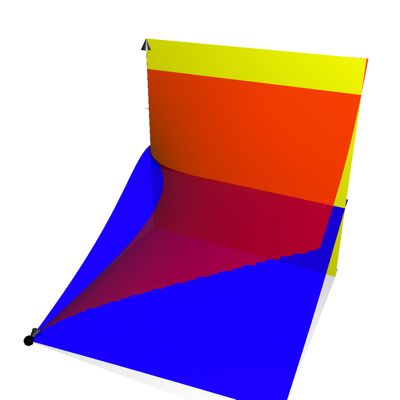
(a) $m=5$

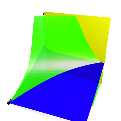
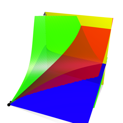
Figure 1: Figures above illustrate the set $\mathcal{S}$ for $m=5$. The variable $Y$ is replaced by a function in $(X_{1},X_{2},Z)$ obtained from (2.9). From readers’ point of view, points in $\mathcal{S}$ are at the front of $X_{1}-X_{2}=0$ (yellow), below $A=0$ (red), behind $B=0$ (green) and above $P=0$ (blue).

The case $m=1$ is very special. In the following proposition, we show that for $m=1$, the defining inequalities $A\geq 0$ and $P\geq 0$ must be equalities. The set $\mathcal{S}$ is closely related to the integral curves $\gamma_{\infty}$ in Remark 3.2 and $\Phi$ in Remark 3.7.

Proposition 4.2.

For $m=1$, the set $\mathcal{S}$ is the union

$$\{p_{0}^{+},p_{2}^{+}\}\cup\gamma_{\infty}\cup\Gamma\cup\left(\Phi\cap\{X_{1},X_{2}>0\}\right).$$

Proof.

It is apparent from Figure 2 that the proposition holds. Consider $\mathcal{S}$ with $m=1$. If $X_{2}=0$ is imposed, we obtain either the point $p_{0}^{+}$ or $\Gamma$ from Proposition 4.1 (a). Hence we assume $X_{2}>0$ in the following. From $A\geq 0$ it is clear that $X_{2}(Y-5Z)\geq YX_{2}-3Z\left(X_{1}+\frac{2}{3}X_{2}\right)\geq 0$ and hence $Y-5Z\geq 0$.

One can easily verify that

$$\begin{split}P&=(X_{1}-X_{2})\left(6YZ-2X_{2}\left(X_{1}+\frac{2}{3}X_{2}\right)\right)-\frac{1}{7}(X_{1}-X_{2})(1-H^{2})-2(Y-Z)A\end{split}.$$ (4.3)

If $X_{1}=X_{2}=X>0$, the first two terms in (4.3) vanish while the last term is non-positive. Then we must have $A=0$, from which we deduce $Y-5Z=0$. By (3.18) we obtain the line segment $\Phi\cap\{X_{1},X_{2}>0\}$.

For $X_{1}\neq X_{2}$, we rewrite (4.3) as follows:

$$\begin{split}P=(X_{1}-X_{2})\left(6YZ-2X_{2}\left(X_{1}+\frac{2}{3}X_{2}\right)-\frac{10}{147}(1-H^{2})\right)-\frac{11}{147}(X_{1}-X_{2})(1-H^{2})-2(Y-Z)A\end{split}.$$ (4.4)

The last two terms in (4.4) are non-positive. Hence from $P\geq 0$ we have

$$\begin{split}0&\leq 6YZ-2X_{2}\left(X_{1}+\frac{2}{3}X_{2}\right)-\frac{10}{147}(1-H^{2})\\ &=6YZ-2X_{2}\left(X_{1}+\frac{2}{3}X_{2}\right)-\frac{10}{147}\left(\frac{7}{6}\left(6Y^{2}+48YZ-12Z^{2}+\frac{12}{7}(X_{1}-X_{2})^{2}\right)-H^{2}\right)\\ &\quad\text{by \eqref{eqn:_new positive conservation law2}}\\ &=\frac{1}{21}(5X_{1}+4X_{2}+5Y+2Z)(X_{1}-X_{2}-Y+5Z)\\ &\quad+\frac{1}{21}\left(5X_{1}+4X_{2}-5Y-2Z\right)(X_{1}-X_{2}+Y-5Z).\end{split}$$ (4.5)

Suppose $X_{1}-X_{2}-Y+5Z\leq 0$, then the first term in the last line of (4.5) is non-positive. As the summation above is non-negative, we know that the second term in the last line of (4.5) must be non-negative. As $X_{1}-X_{2}+Y-5Z\geq 0$, we must have $\frac{1}{5}\left(5X_{1}+4X_{2}-2Z\right)\geq Y$. From $A\geq 0$ we have

$$\frac{X_{2}}{5}\left(5X_{1}+4X_{2}-2Z\right)\geq 3Z\left(X_{1}+\frac{2}{3}X_{2}\right)\Leftrightarrow(5X_{1}+4X_{2})(X_{2}-3Z)\geq 0\Leftrightarrow X_{2}-3Z\geq 0.$$

Then we claim that the first term in (4.3) is non-positive since

$$\begin{split}6YZ-2X_{2}\left(X_{1}+\frac{2}{3}X_{2}\right)&\leq\frac{6}{5}\left(5X_{1}+4X_{2}-2Z\right)Z-2X_{2}\left(X_{1}+\frac{2}{3}X_{2}\right)\\ &\leq\frac{2}{5}\left(5X_{1}+4X_{2}-\frac{2}{3}X_{2}\right)X_{2}-2X_{2}\left(X_{1}+\frac{2}{3}X_{2}\right)\\ &=0.\end{split}$$ (4.6)

But $P\geq 0$. Hence assumptions $X_{1}\neq X_{2}$ and $X_{1}-X_{2}-Y+5Z\leq 0$ lead to the vanishing of $A$ and $P$.

Suppose $X_{1}-X_{2}-Y+5Z\geq 0$. Then $A\geq 0$ implies

$$(X_{1}-X_{2}+5Z)X_{2}\geq 3Z\left(X_{1}+\frac{2}{3}X_{2}\right)\Leftrightarrow X_{2}\geq 3Z.$$

Then we claim that the first term in (4.3) is also non-positive since

$$\begin{split}6YZ-2X_{2}\left(X_{1}+\frac{2}{3}X_{2}\right)&\leq 6(X_{1}-X_{2}+5Z)Z-2X_{2}\left(X_{1}+\frac{2}{3}X_{2}\right)\\ &\leq 2\left(X_{1}-X_{2}+\frac{5}{3}X_{2}\right)X_{2}-2X_{2}\left(X_{1}+\frac{2}{3}X_{2}\right)\\ &=0.\end{split}$$ (4.7)

Hence the assumption $X_{1}\neq X_{2}$ and $X_{1}-X_{2}-Y+5Z\geq 0$ also leads to the vanishing of $A$ and $P$.

Therefore, points in $\mathcal{S}$ with $X_{1}\neq X_{2}$ must have vanished $A$ and $P$, which leads to the following equalities.

$$H=1,\quad 3Z=X_{2},\quad 3Y=3X_{1}+2X_{2}.$$

Note that the last two equations above are equivalent to the defining equations in (3.4) for $m=1$. We obtain $\gamma_{\infty}$ and critical points $p_{0}^{+}$ and $p_{2}^{+}$. ∎

Remark 4.3.

For $m=1$, there is another heterocline $\chi$ that also lies on the invariant set $\mathcal{B}_{\mathrm{Spin}(7)}$. The integral curve joins $q_{3}^{+}$ and $p_{2}^{+}$. Note that from the proof to Proposition 4.2, it is clear that $X_{1}-X_{2}$ and $Y-5Z$ are positive along $\gamma_{\infty}$. These two polynomials are negative along $\chi$ and hence the integral curve is not in $\mathcal{S}$.

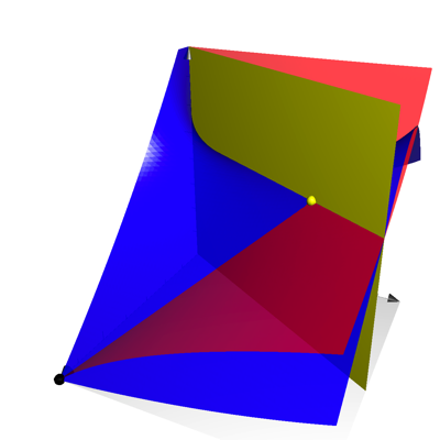
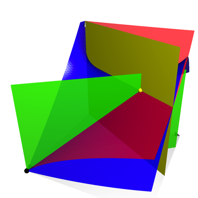
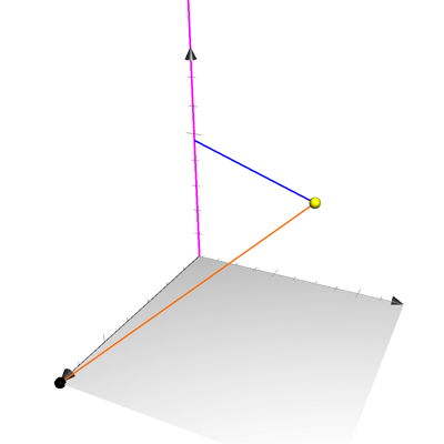
Figure 2: Figures above illustrate the set $\mathcal{S}$ for $m=1$ in the $X_{1}X_{2}Z$-space. The set $\mathcal{S}$ is a 1-dimensional set as shown in the last figure. The orange line segment is $\gamma_{\infty}$ that joins $p_{0}^{+}$ (black) and $p_{2}^{+}$ (yellow), the blue line is part of $\Phi$ and the magenta line is the non-compact part of $\mathcal{S}$ with vanished $X_{1}$ and $X_{2}$.

With Proposition 4.2 established, we can take $m=1$ as our “initial case” for further analysis of cases with $m>1$. In particular, we prove the following technical proposition.

Proposition 4.4.

For $m\geq 1$, the inequality $Q\geq 0$ holds on the set $\mathcal{S}\cap\{P=0\}$. For $m=1$, the inequality reaches equality only at $\{p_{0}^{+},p_{2}^{+}\}\cup\gamma_{\infty}\cup\Gamma$. For $m\geq 2$, the inequality reaches equality only at $p_{0}^{+}$, a point on $\Phi$, and points in $\Gamma$.

Proof.

We consider $\mathcal{S}\cap\{P=0\}$ as a union of slices

$$\mathcal{S}\cap\{P=0\}=\bigcup_{\kappa\in[0,1]}\mathcal{L}_{\kappa},\quad\mathcal{L}_{\kappa}:=\mathcal{S}\cap\{P=0\}\cap\{X_{2}-\kappa X_{1}=0\}.$$

Note that each $\mathcal{L}_{\kappa}$ contains $\Gamma$. As $X_{1}\geq X_{2}\geq 0$ in $\mathcal{S}$, the function $Q$ vanishes once $X_{1}$ does. We assume $X_{1}>0$ in the following discussion.

For $\mathcal{L}_{0}$, we have

$$\left.Q\right|_{\mathcal{L}_{0}}=-2(4m+8)X_{1}YZ+2X_{1}\frac{1-H^{2}}{n}.$$

From $A\geq 0$ we have $Z=0$. Then $\left.Q\right|_{\mathcal{L}_{0}}=2X_{1}\frac{1-H^{2}}{n}$, and $P=0$ becomes $-X_{1}\frac{1-H^{2}}{n}=0$. Hence $\mathcal{L}_{0}=\Gamma\cup\{p_{0}^{+}\}$ and $\left.Q\right|_{\mathcal{L}_{0}}=0$.

If $\kappa=1$, let $X:=X_{1}=X_{2}>0$. Then $A\geq 0$ and $P=0$ respectively become

$$X\left(Y-\frac{2m+3}{m}Z\right)\geq 0,\quad X(Y-(2m+3)Z)(Y-Z)=0.$$

For $X>0$ we must have $Y=(2m+3)Z$. Then from (2.9) we find that $Y=(2m+3)Z=(2m+3)z_{0}$. Hence $\mathcal{L}_{1}$ is a union of $\Gamma$ and a part of the invariant set (3.18). More specifically, from $B\geq 0$ we have

$$\begin{split}\frac{1}{n}-nX^{2}-\frac{2n^{2}(2m+3)(m-1)}{m(2m+1)(8m+3)}YZ=\frac{1}{n}-nX^{2}-\frac{2n^{2}(2m+3)^{2}(m-1)}{m(2m+1)(8m+3)}z_{0}^{2}\geq 0\end{split}.$$ (4.8)

and it follows that

$$\mathcal{L}_{1}=\Gamma\cup\left(\Phi\cap\left\{0<X\leq\frac{1}{n}\sqrt{\frac{36m^{3}+90m^{2}+117m+54}{m(8m+3)(4m^{2}+14m+9)}}\leq\frac{1}{n}\right\}\right)$$ (4.9)

for $m\geq 2$. For $m=1$, we have

$$\mathcal{L}_{1}=\Gamma\cup\left(\Phi\cap\left\{0<X\leq\frac{1}{n}\right\}\right)\cup\{p_{2}^{+}\}.$$ (4.10)

And $\left.Q\right|_{\mathcal{L}_{1}}$ becomes

$$\begin{split}&\left.Q\right|_{\mathcal{L}_{1}}\\ &=X\left(-4Y^{2}-(4m+8)(4m+2)YZ+(n+1)\left(\frac{1}{n}-nX^{2}\right)+4\left(1+\frac{2m}{3}\right)\left(n+\frac{2m}{3}\right)X^{2}\right)\\ &=X\left(-4(2m+3)^{2}z_{0}^{2}-(4m+8)(4m+2)(2m+3)z_{0}^{2}+\frac{n+1}{n}-\frac{4}{9}m(8m+3)X^{2}\right)\\ &=\frac{4}{9}m(8m+3)X\left(\frac{1}{n^{2}}\frac{36m^{3}+90m^{2}+117m+54}{m(8m+3)(4m^{2}+14m+9)}-X^{2}\right)\\ &\geq 0.\end{split}$$ (4.11)

Hence for $m\geq 1$, the function $\left.Q\right|_{\mathcal{L}_{1}}\geq 0$ and it only vanishes on $\Gamma$ and boundary points of $\mathcal{L}_{1}\cap\Phi$. Note that for $m=1$, one of the boundary points of $\mathcal{L}_{1}\cap\Phi$ is $p_{2}^{+}$.

For each $\mathcal{L}_{\kappa}$ with $\kappa\in(0,1)$, replace $X_{2}$ with $X_{1}\kappa$. Then (2.9) and $P=0$ respectively become

$$\begin{split}&\frac{n-1}{n}-\frac{12m}{n}(1-\kappa)^{2}X_{1}^{2}=6Y^{2}+4m(4m+8)YZ-12mZ^{2},\\ &\frac{\kappa-1}{n}-\frac{\kappa-1}{3n}(32\kappa^{2}m^{2}-12\kappa^{2}m+48m\kappa-18\kappa+27)X_{1}^{2}=2\kappa Y^{2}-(4m+8)YZ+(4m\kappa+6)Z^{2}.\end{split}$$ (4.12)

With the equations above, we can write the constant $1$ as a homogeneous polynomial $One(Y,Z)$ of degree $2$. Multiplying the constant term in $B$ by $One(Y,Z)$, the function $B$ restricted to each $\mathcal{L}_{\kappa}\cap\{P=0\}$ then becomes a homogeneous polynomial in $Y$ and $Z$. Factor out $X_{1}$ in $Q$ and multiply the constant term in $\frac{Q}{X_{1}}$ by $One(Y,Z)$. We see that $Q$ restricted on each $\mathcal{L}_{\kappa}\cap\{P=0\}$ is a homogeneous polynomial in $X_{1}$, $Y$ and $Z$. In summary, we have

$$\begin{split}&\left.A\right|_{\mathcal{L}_{\kappa}\cap\{P=0\}}=X_{1}\left(Y\kappa-\frac{3}{m}Z\left(1+\frac{2m}{3}\kappa\right)\right),\\ &\left.B\right|_{\mathcal{L}_{\kappa}\cap\{P=0\}}=b_{2}Z^{2}+b_{1}YZ+b_{0}Y^{2},\quad\left.Q\right|_{\mathcal{L}_{\kappa}\cap\{P=0\}}=X_{1}(q_{2}Z^{2}+q_{1}YZ+q_{0}Y^{2}).\end{split}$$ (4.13)

The coefficients $b_{i}$ and $q_{i}$ in (4.13) are rational functions in $m$ and $\kappa$. Explicit formulas for each coefficient are presented in the Appendix for the sake of simplicity. As $Y$ is positive in $\mathcal{S}$ from Proposition 4.1, we factor out $Y$ and consider $\left.A\right|_{\mathcal{L}_{\kappa}\cap\{P=0\}}=X_{1}Y\tilde{A}_{m,\kappa}\left(\frac{Z}{Y}\right)$, $\left.B\right|_{\mathcal{L}_{\kappa}\cap\{P=0\}}=Y^{2}\tilde{B}_{m,\kappa}\left(\frac{Z}{Y}\right)$ and $\left.Q\right|_{\mathcal{L}_{\kappa}\cap\{P=0\}}=X_{1}Y^{2}\tilde{Q}_{m,\kappa}\left(\frac{Z}{Y}\right)$, where

$$\tilde{A}_{m,\kappa}(x)=\kappa-\left(\frac{3}{m}+2\kappa\right)x,\quad\tilde{B}_{m,\kappa}(x)=b_{2}x^{2}+b_{1}x+b_{0},\quad\tilde{Q}_{m,\kappa}(x)=q_{2}x^{2}+q_{1}x+q_{0}.$$ (4.14)

We have

$$q_{2}=-\frac{4(2\kappa m+3)(32\kappa^{3}m^{3}+\kappa^{2}m^{2}(96-68\kappa)+\kappa m(90-84\kappa)+27(1-\kappa))}{3(1-\kappa)(2\kappa^{2}m(8m-5)+6\kappa(4m-1)+9)}\leq 0$$ (4.15)

for any $(m,\kappa)\in[1,\infty)\times(0,1)$. Therefore, the restricted function $\left.Q\right|_{\mathcal{L}_{\kappa}\cap\{P=0\}}$ is non-negative if it is so on the boundary of $\mathcal{L}_{\kappa}\cap\{P=0\}$. The upper bound and the lower bound of $\frac{Z}{Y}$ on each slice are respectively provided by $\left.A\right|_{\mathcal{L}_{\kappa}\cap\{P=0\}}\geq 0$ and $\left.B\right|_{\mathcal{L}_{\kappa}\cap\{P=0\}}\geq 0$. Specifically, from $\left.A\right|_{\mathcal{L}_{\kappa}\cap\{P=0\}}\geq 0$ we have $\frac{Z}{Y}\leq\frac{m\kappa}{3+2m\kappa}$. As shown in (6.10), we have $b_{2}<0$. By Proposition 6.1 in the Appendix, the smaller real root $\sigma(m,\kappa)$ of $\tilde{B}_{m,\kappa}$ is in the interval $(0,\frac{m\kappa}{3+2m\kappa})$. Hence from $\left.B\right|_{\mathcal{L}_{\kappa}\cap\{P=0\}}\geq 0$ we have $\frac{Z}{Y}\geq\sigma(m,\kappa)$. By the arbitrariness of $\kappa$, it is clear that the minimizing point of $Q$ on ${\mathcal{S}\cap\{P=0\}}$ lies on $\mathcal{S}\cap\{P=0\}\cap\{A=0\}$ or $\mathcal{S}\cap\{P=0\}\cap\{B=0\}$.

We have

$$\begin{split}\left.Q\right|_{\mathcal{L}_{\kappa}\cap\{A=0\}}&=X_{1}Y^{2}\tilde{Q}_{m,\kappa}\left(\frac{m\kappa}{3+2m\kappa}\right)\\ &=X_{1}Y^{2}\frac{4(m+3)(m-1)(4\kappa^{3}m^{2}(8m-1)+4\kappa^{2}m(8m-3)+18\kappa m+9(1-\kappa))\kappa^{2}}{3(2\kappa m+3)(1-\kappa)(2\kappa^{2}m(8m-5)+6\kappa(4m-1)+9)}\\ &\geq 0.\end{split}$$ (4.16)

Therefore, for $m\geq 2$, the function $Q$ is positive on $\mathcal{L}_{\kappa}\cap\{A=0\}$ for any $\kappa\in(0,1)$. For $m=1$, the function $Q$ vanishes at $\mathcal{S}\cap\{P=0\}\cap\{A=0\}$.

Proving the non-negativity of $\left.Q\right|_{\mathcal{L}_{\kappa}\cap\{B=0\}\cap\{P=0\}}$ is a bit more computationally involved. From Proposition 4.2, we know that for $m=1$, the polynomial $A$, $B$ and $P$ identically vanish at $\gamma_{\infty}$. Therefore, an explicit formula for the root $\sigma(1,\kappa)$ can be obtained from $A=0$. We have

$$\sigma(1,\kappa)=\frac{Z}{Y}=\frac{X_{2}}{3\left(X_{1}+\frac{2}{3}X_{2}\right)}=\frac{\kappa}{2\kappa+3}.$$

Define the function $F(m,\kappa):=\tilde{Q}_{m,\kappa}(\sigma(m,\kappa))$. To show that $\left.Q\right|_{\mathcal{L}_{\kappa}\cap\{P=0\}\cap\{B=0\}}\geq 0$, it suffices to show that $F(m,\kappa)\geq 0$ for any $(m,\kappa)\in[1,\infty)\times(0,1)$. Note that the vanishing of $F(m,\kappa)$ means $\sigma(m,\kappa)$ being also a root of $\tilde{Q}_{m,\kappa}$. From the computation (4.16) we have

$$F(1,\kappa):=\tilde{Q}_{1,\kappa}(\sigma(1,\kappa))=\tilde{Q}_{1,\kappa}\left(\frac{\kappa}{3+2\kappa}\right)=0$$

for any $\kappa\in(0,1)$. Furthermore, by implicit derivative, we have

$$\left(\frac{\partial\sigma}{\partial m}\right)(1,\kappa)=\left(-\frac{\frac{\partial b_{2}}{\partial m}\sigma^{2}+\frac{\partial b_{1}}{\partial m}\sigma+\frac{\partial b_{0}}{\partial m}}{2b_{2}\sigma+b_{1}}\right)(1,\kappa)=-\frac{(92\kappa^{4}+1202\kappa^{3}+1458\kappa^{2}-367\kappa-537)\kappa}{66(3+4\kappa)(\kappa+1)(3+2\kappa)^{2}},$$

and it follows that

$$\left(\frac{\partial F}{\partial m}\right)(1,\kappa)=\left(\frac{\partial q_{2}}{\partial m}\sigma^{2}+\frac{\partial q_{1}}{\partial m}\sigma+\frac{\partial q_{0}}{\partial m}+2q_{2}\sigma\frac{\partial\sigma}{\partial m}+q_{1}\frac{\partial\sigma}{\partial m}\right)(1,\kappa)=\frac{4(\kappa-1)(184\kappa^{2}-244\kappa-339)\kappa^{2}}{99(3+4\kappa)(\kappa+1)(2\kappa+3)}>0.$$

Hence $F\geq 0$ on a neighborhood around $\{(1,\kappa)\mid\kappa\in(0,1)\}\subset[1,\infty)\times(0,1)$. In other words, for an $m$ that is slightly larger than $1$, the root $\sigma(m,\kappa)$ of $\tilde{B}_{m,\kappa}$ is strictly between the two real roots of $\tilde{Q}_{m,\kappa}$. Hence proving $F\geq 0$ on $[1,\infty)\times(0,1)$ is equivalent to showing that $\sigma(m,\kappa)$ stays between the two real roots of $\tilde{Q}_{m,\kappa}$ for varying $(m,\kappa)$. This idea leads us to consider the resultant $r(\tilde{Q}_{m,\kappa},\tilde{B}_{m,\kappa})$ for the two polynomials. We have

$$\begin{split}r(\tilde{Q}_{m,\kappa},\tilde{B}_{m,\kappa})&=-\frac{64\kappa^{2}(m-1)(2\kappa m+3)}{(8m+3)^{2}(2m+1)^{2}m^{2}(1-\kappa)(2\kappa^{2}m(8m-5)+6\kappa(4m-1)+9)^{2}}\tilde{r},\\ \tilde{r}&=262144\kappa^{4}m^{10}+(516096\kappa^{4}+679936\kappa^{3})m^{9}+(373760\kappa^{4}+1233920\kappa^{3}+675840\kappa^{2})m^{8}\\ &\quad+(-275904\kappa^{4}+1151040\kappa^{3}+1143744\kappa^{2}+308160\kappa)m^{7}\\ &\quad+(-926496\kappa^{4}+248832\kappa^{3}+1432512\kappa^{2}+507456\kappa+54432)m^{6}\\ &\quad+(-800496\kappa^{4}-1256256\kappa^{3}+1472688\kappa^{2}+857520\kappa+92016)m^{5}\\ &\quad+(-281880\kappa^{4}-1525392\kappa^{3}+266328\kappa^{2}+1353024\kappa+199584)m^{4}\\ &\quad+(-33048\kappa^{4}-644436\kappa^{3}-672624\kappa^{2}+957420\kappa+375192)m^{3}\\ &\quad+(-90396\kappa^{3}-433026\kappa^{2}+186624\kappa+333882)m^{2}\\ &\quad+(-74358\kappa^{2}-59049\kappa+133407)m+19683(1-\kappa).\end{split}$$ (4.17)

As verified in Proposition 6.2 in the Appendix, the inequality $r(\tilde{Q}_{m,\kappa},\tilde{B}_{m,\kappa})\leq 0$ is valid for any $(m,\kappa)\in[1,\infty)\times(0,1)$. Furthermore, the function $r(\tilde{Q}_{m,\kappa},\tilde{B}_{m,\kappa})$ vanishes if and only if $m=1$. In particular, both $\tilde{Q}_{1,\kappa}$ and $\tilde{B}_{1,\kappa}$ have $\sigma(1,\kappa)=\frac{\kappa}{2\kappa+3}$ as their roots. For $m>1$, the polynomials $\tilde{Q}_{m,\kappa}$ and $\tilde{B}_{m,\kappa}$ do not share any common root. Hence $F\geq 0$ on $[1,\infty)\times(0,1)$ and the function $F$ vanishes if and only if $m=1$. Therefore, for $m\geq 2$, the inequality $\left.Q\right|_{\mathcal{L}_{\kappa}\cap\{P=0\}\cap\{B=0\}}\geq 0$ is valid and the equality is reached only at $p_{0}^{+}$ and a point $\Phi\cap\{B=0\}$. The proof is complete. ∎

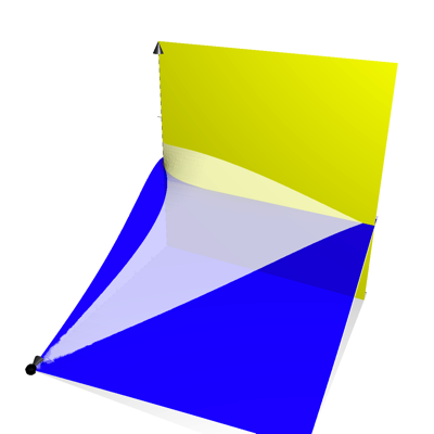
(a) $\mathcal{S}\cap\{P=0\}\cap\{Q\geq 0\}$

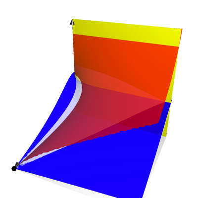
(b) $\mathcal{S}\cap\{P=0\}\cap\{A\geq 0\}\cap\{Q\geq 0\}$

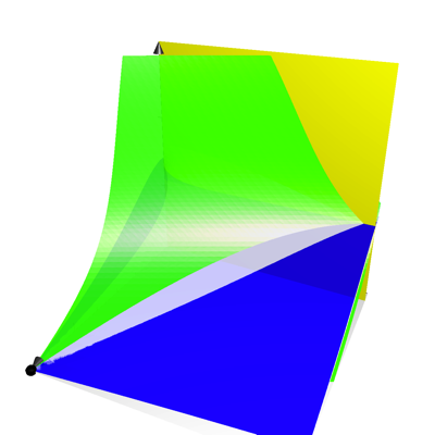
(c) $\mathcal{S}\cap\{P=0\}\cap\{B\geq 0\}\cap\{Q\geq 0\}$

Figure 3: Figures above illustrate Proposition 4.4 for $m=5$. Points in $\mathcal{S}\cap\{P=0\}$ (blue) are at the front ot $\{X_{1}-X_{2}=0\}$ (yellow), below $\{A=0\}$ (red) and behind $\{B=0\}$ (green). Proposition 4.4 shows that $\mathcal{S}\cap\{P=0\}$ is below $\mathcal{S}\cap\{Q=0\}$ (white).

With the help of the proceeding proposition, we are ready to prove the following lemma.

Lemma 4.5.

For $m\geq 2$, integral curves $\gamma_{s_{1}}$ that are in the interior of $\mathcal{S}$ can only escape through some point in $\mathcal{E}\cap\{H\geq 0\}\cap\{X_{1}-X_{2}=0\}$.

Proof.

The boundary $\partial\mathcal{S}$ is a union of the following five sets:

$$\mathcal{S}\cap\{X_{1}-X_{2}=0\},\quad\mathcal{S}\cap\{X_{2}=0\},\quad\mathcal{S}\cap\{A=0\},\quad\mathcal{S}\cap\{B=0\},\quad\mathcal{S}\cap\{P=0\}.$$

By Proposition 4.1, if a $\gamma_{s_{1}}$ escapes $\mathcal{S}$ through some point with vanished $X_{2}$-coordinate, the point must lie in $\mathcal{S}\cap\{A=0\}\cap\{P=0\}$. Hence we aim to show that $V$ points inward when restricted to the last three parts of $\partial\mathcal{S}$.

A straightforward computation shows that

$$\begin{split}&\left.\left\langle\nabla A,V\right\rangle\right|_{A=0}\\ &=A\left(2H\left(G+\frac{1}{n}(1-H^{2})\right)-2X_{1}-(4m+2)X_{2}\right)+\frac{A}{X_{1}+\frac{2m}{3}X_{2}}\left(R_{1}+\frac{2m}{3}R_{2}-\left(1+\frac{2m}{3}\right)\frac{1}{n}(1-H^{2})\right)\\ &\quad+\frac{Y}{X_{1}+\frac{2m}{3}X_{2}}P\\ &=\frac{Y}{X_{1}+\frac{2m}{3}X_{2}}P\quad\text{since $A=0$}\\ &\geq 0.\end{split}$$ (4.18)

It is confirmed that $\left.V\right|_{A=0}$ points inward $\mathcal{S}$.

Since

$$\begin{split}&\left.\left\langle\nabla B,V\right\rangle\right|_{B=0}\\ &=-2\frac{H}{n}(H^{2}-1)\left(G+\frac{1}{n}(1-H^{2})\right)-\frac{2n^{2}(2m+3)(m-1)}{m(16m^{2}+14m+3)}YZ\left(2H\left(G+\frac{1}{n}(1-H^{2})\right)-2X_{2}\right)\\ &\quad\text{by \eqref{eqn:_derivative of H}}\\ &=2BH\left(G+\frac{1}{n}(1-H^{2})\right)+\frac{4n^{2}(2m+3)(m-1)}{m(16m^{2}+14m+3)}YZX_{2}\\ &=\frac{4n^{2}(2m+3)(m-1)}{m(16m^{2}+14m+3)}YZX_{2}\quad\text{since $B=0$}\\ &\geq 0,\end{split}$$ (4.19)

it is clear that $\left.V\right|_{B=0}$ points inward $\mathcal{S}$.

Since

$$\begin{split}&\left.\langle\nabla P,V\rangle\right|_{P=0}\\ &=P\left(H\left(3G+\frac{3}{n}(1-H^{2})-1\right)+\frac{4m}{3}X_{2}\right)+(X_{1}-X_{2})Q\\ &=(X_{1}-X_{2})Q\quad\text{since $P=0$}\\ &\geq 0\quad\text{by Proposition \ref{prop: Q is nonnegative}},\end{split}$$ (4.20)

we learn that $\left.V\right|_{P=0}$ also points inward $\mathcal{S}$.

Finally, we need to exclude the possibility of non-transversal passing of a $\gamma_{s_{1}}$ through some point with $X_{1}\neq X_{2}$. By (4.19) and Proposition 4.1, such a point does not exist on $\mathcal{S}\cap\{B=0\}$. Suppose there were such a point on $\mathcal{S}\cap\{P=0\}$, then $P=Q=0$ at that point by (4.20). Then by Proposition 4.4, we know that such a point is either $p_{0}^{+}$ or a point on $\Phi$, which is impossible. Suppose the non-transversal passing point exists on $\mathcal{S}\cap\{A=0\}$, then by (4.18) and Proposition 4.1, we must have $A=P=0$ at that point, which is also impossible. ∎

To show that some $\gamma_{s_{1}}$ is initially in the set $\mathcal{S}$ we need the following technical proposition.

Proposition 4.6.

Define $\check{A}:=YX_{2}-\frac{m+2}{m}Z\left(X_{1}+\frac{2m}{3}X_{2}\right)$. For $m\geq 2$, the function $Q$ is positive on the set

$$\check{\mathcal{S}}=\mathcal{E}\cap\{X_{1}-X_{2}>0\}\cap\{X_{2}>0\}\cap\{A>0\}\cap\{\check{A}<0\}\cap\{P<0\}.$$

Proof.

We consider $\check{\mathcal{S}}$ as a union of slices

$$\check{\mathcal{S}}=\bigcup_{\kappa\in(0,1)}\check{\mathcal{L}}_{\kappa},\quad\check{\mathcal{L}}_{\kappa}:=\check{\mathcal{S}}\cap\{X_{2}-\kappa X_{1}=0\}.$$

For each $\check{\mathcal{L}}_{\kappa}$ with $\kappa\in(0,1)$, replace $X_{2}$ with $\kappa X_{1}$. Then from (2.9) and $P<0$ we have

$$\begin{split}0&>\left(\frac{1-\kappa}{3n}(32\kappa^{2}m^{2}-12\kappa^{2}m+48m\kappa-18\kappa+27)-\frac{12m}{n(n-1)}(1-\kappa)^{3}\right)X_{1}^{2}\\ &\quad-\left(2\kappa+\frac{6(1-\kappa)}{n-1}\right)Y^{2}+(4m+8)\left(1-4m\frac{1-\kappa}{n-1}\right)YZ+\left(\frac{1-\kappa}{n-1}12m-(4m\kappa+6)\right)Z^{2}\\ &=\frac{(1-\kappa)(16\kappa^{2}m^{2}-10\kappa^{2}m+24\kappa m-6\kappa+9)}{6m+3}X_{1}^{2}\\ &\quad-\left(2\kappa+\frac{6(1-\kappa)}{n-1}\right)Y^{2}+(4m+8)\left(1-4m\frac{1-\kappa}{n-1}\right)YZ+\left(\frac{1-\kappa}{n-1}12m-(4m\kappa+6)\right)Z^{2}.\end{split}$$ (4.21)

The coefficient for $X_{1}^{2}$ in (4.21) is obviously positive for any $(m,\kappa)\in[2,\infty)\times(0,1)$. On the other hand, use (2.9) to replace the constant term in $Q$ with homogeneous polynomials in $X_{1}$, $Y$, and $Z$. The polynomial $Q$ restricted on $\check{\mathcal{L}}_{\kappa}$ becomes

$$\begin{split}\left.Q\right|_{\check{\mathcal{L}}_{\kappa}}&=\frac{-64\kappa^{3}m^{3}+(40\kappa-96)\kappa^{2}m^{2}+(36\kappa^{2}+60\kappa-108)\kappa m+54(\kappa-1)}{18m+9}X_{1}^{3}\\ &\quad+X_{1}\left(\left(2\kappa+\frac{6}{2m+1}\right)Y^{2}-\frac{8m+16}{2m+1}YZ-\left(12m\kappa+\frac{12m}{2m+1}\right)Z^{2}\right).\end{split}$$ (4.22)

It is obvious that the coefficient for $X_{1}^{3}$ in (4.22) is negative for any $(m,\kappa)\in[2,\infty)\times(0,1)$. Note that if (4.21) reaches equality, then one can write $X_{1}^{2}$ as a homogeneous polynomial in $Y$ and $Z$. Moreover, substituting the $X_{1}^{2}$ by the homogeneous polynomial in (4.22) gives the formula for $X_{1}Y^{2}\tilde{Q}\left(\frac{Z}{Y}\right)$ as in (4.14). Therefore, from (4.21) we obtain

$$\left.Q\right|_{\check{\mathcal{L}}_{\kappa}}>X_{1}Y^{2}\tilde{Q}\left(\frac{Z}{Y}\right).$$

Note that $\tilde{Q}\left(\frac{Z}{Y}\right)$ above is defined on $\check{\mathcal{S}}$ instead of $\mathcal{S}\cap\{P=0\}$. On the other hand, the inequalities $A>0$ and $\check{A}<0$ become

$$\frac{3m\kappa}{3(m+2)+2m(m+2)\kappa}<\frac{Z}{Y}<\frac{m\kappa}{3+2m\kappa}.$$

As shown in (4.15), it is clear that the coefficient $q_{2}$ is negative. It suffices to show that $\tilde{Q}$ is positive at $\frac{m\kappa}{3+2m\kappa}$ and $\frac{3m\kappa}{3(m+2)+2m(m+2)\kappa}$ to prove that the polynomial is positive on the open interval in between. From (4.16) it is clear that $\tilde{Q}\left(\frac{m\kappa}{3+2m\kappa}\right)>0$. For any $(m,\kappa)\in[2,\infty)\times(0,1)$, a straightforward computation shows that

$$\begin{split}&\tilde{Q}\left(\frac{3m\kappa}{3(m+2)+2m(m+2)\kappa}\right)\\ &=\frac{512(m-1)\kappa^{2}}{3(1-\kappa)(2\kappa m+3)(2\kappa^{2}m(8m-5)+6\kappa(4m-1)+9)(m+2)^{2}}\left(\left(m^{3}+\frac{11}{8}m^{2}-\frac{19}{4}m-\frac{3}{8}\right)m^{2}\kappa^{3}\right.\\ &\quad\left.+\frac{3}{2}\left(m^{3}-\frac{5}{8}m^{2}+3m-\frac{3}{4}\right)m\kappa^{2}+\left(\frac{9}{8}m^{3}-\frac{99}{64}m^{2}+\frac{27}{16}m-\frac{27}{32}\right)\kappa+\left(\frac{27}{64}m^{2}+\frac{27}{32}\right)\right)\\ &>0.\end{split}$$ (4.23)

The proof is complete. ∎

We are ready to prove the following lemma.

Lemma 4.7.

For $m\geq 2$, the integral curve $\gamma_{s_{1}}$ is initially inside the interior of $\mathcal{S}$ if $s_{1}\in\left(\frac{3}{m-1},\frac{9(5m+3)(4m^{2}+4m+3)}{n^{2}(2m+3)(m-1)}\right)$.

Proof.

With the linearized solution (3.1), we have

$$\begin{split}X_{1}(\gamma_{s_{1}})&=\frac{1}{3}-(8m^{2}+18m+18+(4m+8)ms_{1})e^{\frac{2}{3}\eta}+O\left(e^{\left(\frac{2}{3}+\epsilon\right)\eta}\right)\\ X_{2}(\gamma_{s_{1}})&=(-9+3s_{1}(m+2))e^{\frac{2}{3}\eta}+O\left(e^{\left(\frac{2}{3}+\epsilon\right)\eta}\right)\\ A(\gamma_{s_{1}})&=\frac{m+3}{m}((m-1)s_{1}-3)e^{\frac{2}{3}\eta}+O\left(e^{\left(\frac{2}{3}+\epsilon\right)\eta}\right)\\ B(\gamma_{s_{1}})&=\frac{2n^{2}(2m+3)(m-1)}{m(2m+1)(8m+3)}\left(\frac{9(5m+3)(4m^{2}+4m+3)}{n^{2}(2m+3)(m-1)}-s_{1}\right)e^{\frac{2}{3}\eta}+O\left(e^{\left(\frac{2}{3}+\epsilon\right)\eta}\right)\\ P(\gamma_{s_{1}})&=O\left(e^{\left(\frac{2}{3}+\epsilon\right)\eta}\right)\\ Q(\gamma_{s_{1}})&=O\left(e^{\left(\frac{2}{3}+\epsilon\right)\eta}\right)\end{split}$$ (4.24)

near $p_{0}^{+}$. Hence functions $X_{2}$, $A$ and $B$ are positive along $\gamma_{s_{1}}$ near $p_{0}^{+}$ if $s_{1}\in\left(\frac{3}{m-1},\frac{9(5m+3)(4m^{2}+4m+3)}{n^{2}(2m+3)(m-1)}\right)$. Furthermore, the last two equalities in (4.24) show that $\nabla P$ and $\nabla Q$ are perpendicular to the linearized solution (3.1) at $p_{0}$. Hence the integral curve $\gamma_{s_{1}}$ is tangent to $\{P=0\}$ and $\{Q=0\}$ for any $s_{1}$. It takes a little bit more work to show that the function $P$ is initially positive along $\gamma_{s_{1}}$. Recall in (4.20), we have

$$P^{\prime}=P\left(H\left(3G+\frac{3}{n}(1-H^{2})-1\right)+\frac{4m}{3}X_{2}\right)+(X_{1}-X_{2})Q.$$ (4.25)

Note that

$$\left(H\left(3G+\frac{3}{n}(1-H^{2})-1\right)+\frac{4m}{3}X_{2}\right)(\gamma_{s_{1}})=-(48m^{2}+84m+20m(m+2)s_{1})e^{\frac{2}{3}\eta}+O\left(e^{\left(\frac{2}{3}+\epsilon\right)\eta}\right)$$

near $p_{0}^{+}$. If $P$ were negative initially along $\gamma_{s_{1}}$ near $p_{0}^{+}$, the first term in (4.25) is positive. Moreover, from the linearized solution (3.1), we have

$$\check{A}(\gamma_{s_{1}})=-\frac{1}{m}\left(6m+6-(m+2)(m-1)s_{1}\right)e^{\frac{2}{3}\eta}+O\left(e^{\left(\frac{2}{3}+\epsilon\right)\eta}\right).$$

Since $\frac{9(5m+3)(4m^{2}+4m+3)}{n^{2}(2m+3)(m-1)}<\frac{6(m+1)}{(m+2)(m-1)}$ for $m\geq 2$, we know that $\check{A}(\gamma_{s_{1}})$ is initially negative along $\gamma_{s_{1}}$. Based on the assumption that $P$ is initially negative along $\gamma_{s_{1}}$, we know that $\gamma_{s_{1}}$ is initially in $\check{\mathcal{S}}$. By Proposition 4.6, we know that the second term in (4.25) is also positive and so is $P^{\prime}$, which is a contradiction. Therefore, the function $P$ must be positive initially along $\gamma_{s_{1}}$ near $p_{0}^{+}$. ∎

According to Section 4 in [Böh98], the existence of the heterocline that joins $p_{0}^{\pm}$ relies on the number of critical points of $\sqrt{\frac{Z}{Y}}$ that appear before the turning point. The number is originally denoted by $\sharp C_{w}(\bar{h})$ in [Böh98], where $w$ is the ratio $\frac{f_{1}}{f_{2}}=\sqrt{\frac{Z}{Y}}$ and $\bar{h}$ corresponds to the initial data $f$ in (2.3). We introduce the following modified definitions of $\sharp C_{w}(\bar{h})$ and $W$-intersection points.

Definition 4.8.

For a $\gamma_{s_{1}}$ that is not a heterocline, i.e., a $\gamma_{s_{1}}$ that is not defined on $\mathbb{R}$ or $\lim\limits_{\eta\to\infty}\gamma_{s_{1}}\neq p_{0}^{-}$, let $\sharp C(\gamma_{s_{1}})$ be the number of critical points of the function $\sqrt{\frac{Z}{Y}}$ along $\gamma_{s_{1}}$ that appear in $\mathcal{E}\cap\{H>0\}\cap\{Y-Z>0\}$.

Definition 4.9.

The point where $\gamma_{s_{1}}$ or $\zeta_{s_{2}}$ intersects $\mathcal{E}\cap\{H>0\}\cap\{Y-Z=0\}$ is called a $W$-intersection point.

We have the following proposition.

Proposition 4.10.

Any $\gamma_{s_{1}}$ with $s_{1}>-3$ (or $\zeta_{s_{2}}$ with $s_{2}>0$) has a turning point at $\mathcal{E}\cap\{H=0\}$ or a $W$-intersection point at $\mathcal{E}\cap\{Y-Z=0\}$.

Proof.

An integral curve $\gamma_{s_{1}}$ with $s_{1}>-3$ (or $\zeta_{s_{2}}$ with $s_{2}>0$) is initially in the interior of the compact set $\mathcal{E}\cap\{H\geq 0\}\cap\{Y-Z\geq 0\}$. Suppose the integral curve does not have any turning point or any $W$-intersection point. Then it must be defined on $\mathbb{R}$. Furthermore, such an integral curve is in $\mathcal{E}\cap\{H<1\}$ initially. From (2.11), along the integral curve we eventually have $H^{2}<1-\epsilon$ for some $\epsilon>0$. Hence

$$H^{\prime}=(H^{2}-1)\left(\frac{1}{n}+\frac{12m}{n}(X_{1}-X_{2})^{2}\right)\leq\frac{H^{2}-1}{n}<-\frac{\epsilon}{n}$$

eventually, meaning the function $H$ must at vanish some point. We reach a contradiction. Each of the integral curve without a turning point must have a $W$-intersection point. ∎

We rephrase Lemma 4.4 in [Böh98] with these new definitions.

Theorem 4.11.

If $\gamma_{s_{1}}$ is not a heterocline for any $s_{1}\in[a,b]$, then $\sharp C(\gamma_{s_{1}})$ is a constant for all $s_{1}\in[a,b]$.

Immediately, we have the following proposition

Proposition 4.12.

The quantities $\sharp C(\gamma_{0})$ and $\sharp C(\zeta_{\frac{1}{2m+6}})$ are both zero.

Proof.

From defining equations of $\mathcal{B}_{QK}$, we have $X_{1}=Y-2Z$ and $X_{2}=-Z$ along $\gamma_{0}$. Then $H^{2}<1$ becomes $(3Y-(n+3)Z)^{2}<1$. From (3.14) we have

$$\begin{split}&\frac{12m}{n}(Y-Z)^{2}+6Y^{2}+4m(4m+8)YZ-12mZ^{2}>\frac{n-1}{n}(3Y-(4m+6)Z)^{2}\\ \Leftrightarrow&n(n+9)(n-1)(Y-Z)Z>0.\end{split}$$ (4.26)

Hence $X_{1}-X_{2}=Y-Z>0$ along $\gamma_{0}$. Similarly, we have $X_{2}-X_{1}=Y-Z>0$ along $\zeta_{\frac{1}{2m+6}}$. Note that $X_{1}-X_{2}$ vanishes at the critical point $p_{1}^{-}$ and it stays positive along $\gamma_{0}$. ∎

We are ready to prove Theorem 1.1.

Proof of Theorem 1.1.

Consider a $\gamma_{s_{1}}$ with $s_{1}\in\left(\frac{3}{m-1},\frac{9(5m+3)(4m^{2}+4m+3)}{n^{2}(2m+3)(m-1)}\right)$. From Lemma 4.7 we know that such a $\gamma_{s_{1}}$ is initially in $\mathcal{S}$. From (2.11) we know that such a $\gamma_{s_{1}}$ must exit $\mathcal{S}$. From Lemma 4.5 we know that such a $\gamma_{s_{1}}$ exits $\mathcal{S}$ through the face $\mathcal{E}\cap\{H>0\}\cap\{Y-Z\geq 0\}\cap\{X_{1}-X_{2}=0\}$. It is clear that $\left(\sqrt{\frac{Z}{Y}}\right)^{\prime}=\sqrt{\frac{Z}{Y}}(X_{1}-X_{2})$. Since $Z$ is initially positive along $\gamma_{s_{1}}$ with $s_{1}>\frac{3}{m-1}$, we know that $\sharp C(\gamma_{s_{1}})$ is exactly the number of times that $\gamma_{s_{1}}$ intersects $\mathcal{E}\cap\{H>0\}\cap\{Y-Z\geq 0\}\cap\{X_{1}-X_{2}=0\}$. Hence $\sharp C(\gamma_{s_{1}})\geq 1$ for $s_{1}\in\left(\frac{3}{m-1},\frac{9(5m+3)(4m^{2}+4m+3)}{n^{2}(2m+3)(m-1)}\right)$.

On the other hand, the integral curve $\gamma_{0}$ joins $p_{0}^{+}$ and $p_{1}^{-}$. From Proposition 4.12, the function $X_{1}-X_{2}$ stays positive along $\gamma_{0}$. Hence we have $\sharp C(\gamma_{0})=0$. Therefore, by Theorem 4.11 there exists some $s_{\star}\in\left(0,\frac{9(5m+3)(4m^{2}+4m+3)}{n^{2}(2m+3)(m-1)}\right)$ such that $\gamma_{s_{\star}}$ is a heterocline that joins $p_{0}^{\pm}$. Theorem 1.1 is proved. ∎

Remark 4.13.

With some small modifications, the polynomial $\mathcal{S}$ can be applied to prove the existence of positive Einstein metrics on $F^{m+1}$, a cohomogeneity one space formed by the group triple $(Sp(m)U(1),Sp(m)Sp(1),Sp(m+1))$. Furthermore, some non-existence results can also be obtained from the defining polynomial $P$. For some cohomogeneity one spaces, the function $P$ is negative along all $\gamma_{s_{1}}$ in $\mathcal{E}\cap\{X_{1}-X_{2}\geq 0\}$, essentially forcing $X_{1}-X_{2}$ to be positive along these integral curves. For example, there is no $\mathrm{Spin}(9)$-invariant cohomogeneity one positive Einstein metric on $\mathbb{OP}^{2}\sharp\overline{\mathbb{OP}}^{2}$. A systematic study of the existence problem on all cohomogeneity one spaces with two isotropy summands will be soon presented in later work.

Remark 4.14.

One can recover Böhm’s metric on $\mathbb{HP}^{2}\sharp\overline{\mathbb{HP}}^{2}$ by enlarging the set $\mathcal{S}$ for $m=1$. Specifically, we can increase the coefficient for $Y$ in the polynomial $A$ properly so that: 1. Integral curves $\gamma_{s_{1}}$ with large enough $s_{1}$ are in the enlarged $\mathcal{S}$ initially. 2. Integral curves that are in the enlarged $\mathcal{S}$ must exit through the face $\mathcal{S}\cap\{X_{1}-X_{2}=0\}$. Note that the derivative of the new polynomial $A$ still depends on the non-negativity of the same polynomial $P$. Hence $\sharp C(\gamma_{s_{1}})\geq 1$ with large enough $s_{1}$ while $\sharp C(\gamma_{0})=0$, and Theorem 4.11 can be applied to prove the existence.

We end this section with the following remark to discuss the motivation in defining $\mathcal{S}$.

Remark 4.15.

Inspired by Corollary 5.8 in [Böh98] and by the fact that $p_{2}^{+}$ is a stable node, we realized that taking the limit $s_{1}\to\infty$ for $\gamma_{s_{1}}$ may not provide enough information to prove the existence theorem for all $m$. From (3.2) we know that $s_{1}$ is related to the initial condition $f$. Numerical data in Table 2 in [Böh98] indicate that the winding angle of $\gamma_{s_{1}}$ around $\Phi$ may not be monotonic as $s_{1}$ increases. Hence it is reasonable to find a bounded interval of $s_{1}$ for which the winding angle of $\gamma_{s_{1}}$ is large enough.

From (4.19) and (4.24), it appears that the upper bound for $s_{1}$ can be easily controlled by changing the coefficient for $YZ$ in $B$. Looking for an appropriate lower bound for $s_{1}$, on the other hand, is relatively more difficult. Originally we choose to obtain the lower bound from $f_{2}\dot{f_{2}}\geq f_{1}\dot{f_{1}}$. The inequality is equivalent to $YX_{2}\geq ZX_{1}$. Although the inequality is geometrically motivated, showing it can be maintained before the winding angle gets large enough seems to be too difficult. We eventually define the polynomial $A$, whose first and second derivatives are relatively easier to be controlled by polynomials $P$ and $Q$.

5 Limiting Winding Angle

From [Win17] we know that $\gamma_{\infty}$ joins $p_{0}^{+}$ and $p_{2}^{+}$. By the symmetry of $\eqref{eqn:_new Positive Einstein system}$, we know that there exists $\bar{\gamma}_{\infty}$ that joins $p_{2}^{-}$ and $p_{0}^{-}$. As $\Phi$ joins $p_{2}^{\pm}$, we have this set of heteroclines $\{\gamma_{\infty},\Phi,\bar{\gamma}_{\infty}\}$ that joins $p_{0}^{\pm}$. From this perspective, the critical point $p_{2}^{+}$ is anticipated to play an important role in the qualitative analysis. Intuitively speaking, if $p_{2}^{+}$ were a stable focus in the Ricci-flat subsystem, the integral curve $\gamma_{s_{1}}$ would wind around $\Phi$ more frequently as $s_{1}$ increases. From Section 3, however, we learn that $p_{2}^{+}$ is a stable node in the Ricci-flat subsystem. Hence the winding behavior of $\gamma_{s_{1}}$ around $\Phi$ is less obvious. The new coordinate change helps us estimate the limiting winding angle of $\gamma_{s_{1}}$ as $s_{1}\to\infty$ and establish Theorem 1.2. On the other hand, another set of heteroclines $\{\zeta_{\infty},\Phi,\bar{\zeta}_{\infty}\}$ joins $p_{1}^{\pm}$. It is natural to ask if some heterocline other than $\zeta_{0}$ joins $p_{1}^{\pm}$. The new coordinate change also helps us to answer this question and prove Theorem 1.3.

We introduce some known estimates in the Ricci-flat system in the following. The Ricci-flat subsystem on $\mathcal{E}\cap\{H=1\}$ is simply a subsystem of (2.16) in [Chi21], with $Y_{1}\to\sqrt{2}$, $Y_{2}\to\sqrt{2}Y$ and $Y_{3}\to 2\sqrt{2}Z$. From Lemma 4.4 in [Chi21], we learn that the compact set

$$\hat{\mathcal{B}}_{RF}:=\mathcal{E}\cap\{H=1\}\cap\{Y-Z\geq 0\}\cap\{X_{2}-X_{1}+2Y-2Z\geq 0\}\cap\left\{X_{1}\leq\frac{1}{2}\right\}\cap\{X_{2}\geq 0\}$$

is invariant. Critical points $p_{0}^{+}$ and $p_{1}^{+}$ are on the boundary of $\hat{\mathcal{B}}_{RF}$ while $p_{2}^{+}$ is in the interior. Straightforward computations show that $\gamma_{\infty}$ and $\zeta_{\infty}$ are initially in $\hat{\mathcal{B}}_{RF}$. From Lemma 5.7 in [Chi21], it is known that these two integral curves converge to $p_{2}^{+}$. We construct the following invariant set introduced in [Chi19], which gives us more information on $\gamma_{\infty}$ near $p_{2}^{+}$.

Proposition 5.1.

The set

$$\mathcal{B}_{RF}:=\mathcal{E}\cap\{H=1\}\cap\{Y-(2m+3)Z\geq 0\}\cap\{X_{2}-X_{1}+Y-(2m+3)Z\geq 0\}$$

is compact and invariant.

Proof.

The compactness is derived from $Y-(2m+3)Z\geq 0$ and (2.9).

Since

$$\begin{split}&\langle\nabla(Y-(2m+3)Z),V\rangle_{\mathcal{B}_{RF}\cap\{Y-(2m+3)Z=0\}}\\ &=(Y-(2m+3)Z)\left(H\left(G+\frac{1}{n}(1-H^{2})\right)-X_{1}-(4m+6)Z\right)\\ &\quad+(4m+6)Z(X_{2}-X_{1}+Y-(2m+3)Z)\\ &=(4m+6)Z(X_{2}-X_{1}+Y-(2m+3)Z)\quad\text{since $Y-(2m+3)Z=0$}\\ &\geq 0,\\ \end{split}$$ (5.1)

the vector field $V$ points inward on the boundary $\mathcal{B}_{RF}\cap\{Y-(2m+3)Z=0\}$. As for $\mathcal{B}_{RF}\cap\{X_{2}-X_{1}+Y-(2m+3)Z=0\}$, from (2.9) we have

$$\begin{split}&\frac{12m}{n}(Y-(2m+3)Z)^{2}+6Y^{2}+4m(4m+8)YZ-12mZ^{2}=\frac{n-1}{n}\\ &\Leftrightarrow 18(2m+1)Y^{2}+8m(8m^{2}+16m+3)YZ+24m(2m^{2}+4m+3)Z^{2}=4m+2.\\ \end{split}$$ (5.2)

Then we have

$$\begin{split}&\langle\nabla(X_{2}-X_{1}+Y-(2m+3)Z),V\rangle_{\mathcal{B}_{RF}\cap\{X_{2}-X_{1}+Y-(2m+3)Z)=0\}}\\ &=(X_{2}-X_{1}+Y-(2m+3)Z))\left(H\left(G+\frac{1}{n}(1-H^{2})-1\right)+\frac{4m}{n}Y+\frac{8m^{2}+24m+18}{n}Z\right)\\ &\quad+\frac{1}{n}(Y-(2m+3)Z)((4m+2)H-(12m+6)Y-(8m^{2}+16m+12)Z)\\ &=\frac{1}{n}(Y-(2m+3)Z)(4m+2-(12m+6)Y-(8m^{2}+16m+12)Z)\\ &\quad\text{since $H=1$ and $X_{2}-X_{1}+Y-(2m+3)Z=0$}.\end{split}$$ (5.3)

With $Y,Z\geq 0$, showing $4m+2-(12m+6)Y-(8m^{2}+16m+12)Z\geq 0$ is equivalent to showing $(4m+2)^{2}\geq((12m+6)Y+(8m^{2}+16m+12)Z)^{2}$. Note that $(4m+2)^{2}$ is simply the LHS of (5.2) multiplied by $4m+2$. Hence one can obtain the non-negativity by verifying

$$\begin{split}&(4m+2)(18(2m+1)Y^{2}+8m(8m^{2}+16m+3)YZ+24m(2m^{2}+4m+3)Z^{2})\\ &\geq((12m+6)Y+(8m^{2}+16m+12)Z)^{2}\\ &\Leftrightarrow\\ &16n(m-1)((4m^{2}+8m+3)YZ+(2m^{2}+4m+3)Z^{2})\geq 0.\end{split}$$ (5.4)

Note that the equality is reached by $m=1$. Hence (5.3) is non-negative and it identically vanishes if $m=1$. Hence $\mathcal{B}_{RF}$ is invariant. ∎

Remark 5.2.

With (2.9) one can easily show that

$$\begin{split}\mathcal{B}_{\mathrm{Spin}(7)}&=\mathcal{E}\cap\{Y-2Z-X_{1}=0\}\cap\{3Z-X_{2}=0\}\\ &=\mathcal{E}\cap\{H=1\}\cap\{X_{2}-X_{1}+Y-5Z=0\}.\end{split}$$ (5.5)

Therefore, the fact that (5.3) identically vanishes for $m=1$ recovers the invariant set $\mathcal{B}_{\mathrm{Spin}(7)}$ as in (3.4).

Remark 5.3.

By (5.1) and (5.3), one can also show that the set

$$\tilde{\mathcal{B}}_{RF}:=\mathcal{E}\cap\{H=1\}\cap\{Y-(2m+3)Z\leq 0\}\cap\{X_{2}-X_{1}+Y-(2m+3)Z\leq 0\}.$$

is also invariant. Furthermore,

Proposition 5.4.

For $m\geq 2$, the integral curve $\gamma_{\infty}$ is in $\mathcal{B}_{RF}$ initially. For $m=1$, the integral curve $\gamma_{\infty}$ stays on the boundary of $\mathcal{B}_{RF}$. For $m\geq 1$, the integral curve $\zeta_{\infty}$ is in $\tilde{\mathcal{B}}_{RF}$ initially.

Proof.

The statement is clear by (3.3) and (3.13). Note that for $m=1$, the function $X_{2}-X_{1}+Y-5Z$ is identically zero on $\gamma_{\infty}$. ∎

To obtain more information on how $\gamma_{s_{1}}$ and $\zeta_{s_{2}}$ wind around $\Phi$ as $s_{1},s_{2}\to\infty$, we consider the following “cylindrical” coordinate.

$$r\sin(\theta)=X_{1}-X_{2},\quad r\cos(\theta)=\sqrt{\frac{2m+2}{2m+3}}(Y-(2m+3)Z).$$

The system (2.7) is transformed into

$$\begin{bmatrix}H\\ r\\ \theta\\ Y\end{bmatrix}^{\prime}=\begin{bmatrix}(H^{2}-1)\left(\frac{1}{n}+\frac{12m}{n}r^{2}\sin^{2}(\theta)\right)\\ rH\left(\frac{1}{n}+\frac{12m}{n}r^{2}\sin^{2}(\theta)\right)-Hr\sin^{2}(\theta)-\frac{H}{n}r\cos^{2}(\theta)+\left(\frac{m+2}{m+1}+\frac{3}{n}\right)r^{2}\sin(\theta)\cos^{2}(\theta)\\ 2\sqrt{\frac{2m+2}{2m+3}}Y+\frac{1}{m+1}r\cos(\theta)-\frac{n-1}{n}H\sin(\theta)\cos(\theta)-\left(\frac{m+2}{m+1}+\frac{3}{n}\right)r\cos(\theta)\sin^{2}(\theta)\\ Y\left(\frac{12m}{n}Hr^{2}\sin^{2}(\theta)-\frac{4m}{n}r\sin(\theta)\right)\end{bmatrix}$$ (5.6)

with conservation law (2.9) rewritten as

$$C_{\Lambda\geq 0}\colon\frac{12m}{n}r^{2}\sin^{2}(\theta)+6Y^{2}+4m(4m+8)Y\tilde{Z}-12m\tilde{Z}^{2}=1-\frac{1}{n},\quad\tilde{Z}=\left(\frac{Y}{2m+3}-\frac{r\cos(\theta)}{\sqrt{(2m+2)(2m+3)}}\right).$$

The set $\mathcal{E}$ is then defined in the $(H,r,\theta,Y)$-coordinate accordingly. The variable $r$ tells the distance from a point to $\Phi$ and $\theta$ records the winding angle around $\Phi$.

With the new conservation law, setting $r=0$ implies $Y=(2m+3)z_{0}$. Restricting (5.6) to the invariant set $\mathcal{E}\cap\{r=0\}$ gives the following subsystem.

$$\begin{bmatrix}H\\ \theta\end{bmatrix}^{\prime}=\begin{bmatrix}(H^{2}-1)\frac{1}{n}\\ 2\sqrt{(2m+2)(2m+3)}z_{0}-\frac{n-1}{n}H\sin(\theta)\cos(\theta)\end{bmatrix},\quad r=0,\quad Y=(2m+3)z_{0}$$ (5.7)

The subsystem above is essentially the integral curve $\Phi$. Straightforward computations show that (5.6) has the following four sequences of critical points in $\mathcal{E}\cap\{r=0\}$:

$$\begin{split}\{A_{i}^{\pm}:=(\pm 1,0,a_{i}^{\pm},(2m+3)z_{0})\}_{i\in\mathbb{Z}},\quad a_{i}^{\pm}=\pm\arctan\left(-\frac{\delta_{1}}{2\sqrt{(2m+3)(2m+2)}z_{0}}\right)+i\pi,\\ \{B_{i}^{\pm}:=(\pm 1,0,b_{i}^{\pm},(2m+3)z_{0})\}_{i\in\mathbb{Z}},\quad b_{i}^{\pm}=\pm\arctan\left(-\frac{\delta_{2}}{2\sqrt{(2m+3)(2m+2)}z_{0}}\right)+i\pi.\end{split}$$ (5.8)

Furthermore, for each $i\in\mathbb{Z}$ we have

$$\begin{split}&a_{i}^{+}\in\left(i\pi,\frac{\pi}{4}+i\pi\right),\quad b_{i}^{+}\in\left(\frac{\pi}{4}+i\pi,\frac{\pi}{2}+i\pi\right),\\ &b_{i}^{-}\in\left(-\frac{\pi}{2}+i\pi,-\frac{\pi}{4}+i\pi\right),\quad a_{i}^{-}\in\left(-\frac{\pi}{4}+i\pi,i\pi\right).\end{split}$$ (5.9)

Remark 5.5.

Computations show that $A_{i}^{+}$’s and $B_{i}^{+}$’s are transformed respectively from the two stable eigenvectors $u_{1}$ and $u_{2}$ of the linearization at $p_{2}^{+}$. Recall from Section 3 that both $u_{1}$ and $u_{2}$ are tangent to $\mathcal{E}\cap\{H=1\}$ and the corresponding eigenvalues $\delta_{1}$ and $\delta_{2}$ are real numbers and we have $\delta_{2}<\delta_{1}<0$. Each linearized solution to the Ricci-flat subsystem around $p_{2}^{+}$ must have $e^{\delta_{2}\eta}\ll e^{\delta_{1}\eta}$ as $\eta\to\infty$. Hence integral curves $\gamma_{\infty}$ and $\zeta_{\infty}$ converge to $p_{2}^{+}$ along $u_{1}$. Hence it is not surprising that $A_{i}^{+}$’s are sinks and $B_{i}^{+}$’s are saddles in the subsystem of (5.6) restricted to $\mathcal{E}\cap\{H=1\}$. Furthermore, for the subsystem (5.7), critical points $A_{i}^{+}$’s are saddles, and $B_{i}^{+}$’s are sources.

Thanks to the invariant set $\mathcal{B}_{RF}$ in Proposition 5.1, whose boundary contains $p_{2}^{+}$. We are now ready to show that both $\gamma_{\infty}$ and $\zeta_{\infty}$ do not wind fully around $p_{2}^{+}$.

Proposition 5.6.

Consider the $(H,r,\theta,Y)$-coordinate. For $m\geq 2$, the integral curve $\gamma_{\infty}$ joins the critical points $p_{0}^{+}$ and $A_{0}^{+}$. For $m=1$, the variable $\theta$ remains a constant along $\gamma_{\infty}$ and the integral curve joins $p_{0}^{+}$ and $B_{0}^{+}$. For $m\geq 1$, the integral curve $\zeta_{\infty}$ joins the critical points $p_{1}^{+}$ and $A_{1}^{+}$.

Proof.

In the new coordinate, the critical point $p_{0}^{+}$ is $\left(1,\frac{1}{3}\sqrt{\frac{4m+5}{2m+3}},\arctan\left(\sqrt{\frac{2m+3}{2m+2}}\right),\frac{1}{3}\right)$. As $\gamma_{\infty}$ joins $p_{0}^{+}$ and $p_{2}^{+}$ in the $(X_{1},X_{2},Y,Z)$-coordinate, it is clear that the integral curve joins $p_{0}^{+}$ and one of $A_{i}^{+}$ or $B_{i}^{+}$ in the new coordinate. From Proposition 5.1 and Proposition 5.4 we know that $r\cos(\theta)\geq 0$ and $\sqrt{\frac{2m+3}{2m+2}}r\cos(\theta)-r\sin(\theta)\geq 0$ along $\gamma_{\infty}$. In particular, the second inequality reaches equality so that $\theta=\arctan\left(\sqrt{\frac{2m+3}{2m+2}}\right)$ along $\gamma_{\infty}$ for $m=1$. Note that $0<a_{0}^{+}<\arctan\left(\sqrt{\frac{2m+3}{2m+2}}\right)\leq b_{0}^{+}$ and the last inequality reaches equality for $m=1$. The $\theta$-coordinate for $p_{0}^{+}$ is positive and $\{\theta\geq 0\}$ is clearly invariant. Hence for $m\geq 2$, the integral curve $\gamma_{\infty}$ converges to $A_{0}^{+}$; for $m=1$, the integral curve $\gamma_{\infty}$ converges to $B_{0}^{+}$ as $\theta=b_{0}^{+}$ along $\gamma_{\infty}$.

In the $(H,r,\theta,Y)$-coordinate, the critical point $p_{1}^{+}$ is $\left(1,\sqrt{\frac{2m+2}{2m+3}}\frac{2m+2}{n},\pi,\frac{1}{n}\right)$. It is established in [Chi21] that $\zeta_{\infty}$ is an integral curve that joins $p_{1}^{+}$ and $p_{2}^{+}$ in the $(X_{1},X_{2},Y,Z)$-coordinate. Therefore, in the $(H,r,\theta,Y)$-coordinate, the integral curve $\zeta_{\infty}$ joins $p_{1}^{+}$ and one of $A_{i}^{+}$’s or $B_{i}^{+}$’s. As $\zeta_{\infty}$ is in $\tilde{\mathcal{B}}_{RF}$ initially, by Remark 5.3 we know that $\cos(\theta)=\sqrt{\frac{2m+2}{2m+3}}(Y-(2m+3)Z)\leq 0$ and $\sqrt{\frac{2m+3}{2m+2}}r\cos(\theta)-r\sin(\theta)\leq 0$ along $\zeta_{\infty}$. Hence we know that $\frac{\pi}{2}\leq\theta\leq\arctan\left(\sqrt{\frac{2m+3}{2m+2}}\right)+\pi\leq b_{1}^{+}$ along $\zeta_{\infty}$. Therefore $\zeta_{\infty}$ converges to $A_{1}^{+}$ for $m\geq 2$. We claim that the integral curve $\zeta_{\infty}$ also converges to $A_{1}^{+}$ for $m=1$. Recall Remark 4.3 and Remark 5.2. The integral curve $\chi$ also converges to $p_{2}^{+}$ and along $\chi$ we have $X_{2}-X_{1}\geq 0$ and $X_{2}-X_{1}+Y-5Z=0$. Hence $\chi$ converges to $B_{1}^{+}$ in the $(H,r,\theta,Y)$-coordinate. As the linearization at $B_{1}^{+}$ has only one stable eigenvector, we know that $\zeta_{\infty}$ converges to $A_{1}^{+}$. ∎

We claim the following lemma.

Lemma 5.7.

Let $\Pi$ be the integral curve of the subsystem (5.7) that emanates from $A_{0}^{+}$. Let $(0,0,\theta_{*},(2m+3)z_{0})$ be the midpoint of $\Pi$ at which it passes through $H=0$. For $m\geq 2$, we have $\theta_{*}=\lim\limits_{s_{1}\to\infty}\theta(\gamma_{s_{1}}\cap\{H=0\})$.

Proof.

We think of (5.6) on $\mathcal{E}$ as a dynamical system in the three dimensional $Hr\theta$-space with $Y$ as a function in $(H,r,\theta)$. As mentioned in Remark 5.5, each $A_{i}^{+}$ is a saddle whose linearization has two stable eigenvectors and one unstable eigenvector. Furthermore, the two stable eigenvectors are parallel to $\mathcal{E}\cap\{H=1\}$, meaning that each $A_{i}^{+}$ is a sink in the Ricci-flat subsystem and $\Pi$ is the only integral curve that emanates from $A_{i}^{+}$ in $\mathcal{E}\cap\{H<1\}$. By Hartman–Grobman theorem, there is a local homeomorphism $(\phi,\mathcal{U})$ defined around $A_{0}^{+}$ through which the system (5.6) is topologically equivalent to the following linear dynamical system

$$\begin{bmatrix}x\\ y\\ z\end{bmatrix}^{\prime}=\begin{bmatrix}-1&0&0\\ 0&-1&0\\ 0&0&1\\ \end{bmatrix}\begin{bmatrix}x\\ y\\ z\end{bmatrix}.$$ (5.10)

In particular, we have

$$\phi(A_{0}^{+})=(0,0,0),\quad\phi(\mathcal{U}\cap\{H=1\})\subset\{(x,y,0)\mid x,y\in\mathbb{R}\},\quad\phi(\mathcal{U}\cap\Pi)\subset\{(0,0,z)\mid z\in\mathbb{R}\}.$$

Let $D_{\epsilon}$ be an open disk on the $xy$-plane with radius $\epsilon_{1}$. Let $U_{1}$ be the cylinder $D_{\epsilon_{1}}\times(-\epsilon_{2},\epsilon_{2}]$. Note that integral curves in $U_{1}\cap\{z>0\}$ can only escape through the face $D_{\epsilon_{1}}\times\{\epsilon_{2}\}$. Choose small enough $\epsilon_{1}$ and $\epsilon_{2}$ so that $\mathcal{U}_{1}:=\phi^{-1}(U_{1})$ is contained in $\mathcal{U}$. Then $p:=\phi^{-1}(0,0,\epsilon_{2})$ is a point on $\mathcal{U}\cap\Pi$.

Let $\mathcal{U}_{0}$ be an open neighborhood around the point $(0,0,\theta_{*})$ in the $Hr\theta$-space. By the continuous dependence, there exists an open set $\mathcal{U}_{2}\ni p$ in $\mathcal{U}$ such that any point in $\mathcal{U}_{2}$ lies on an integral curve that enters $\mathcal{U}_{0}$. It is clear that $p\in\mathcal{U}_{1}\cap\mathcal{U}_{2}$. Modify $U_{1}$ by shrinking $\epsilon_{1}$ so that $D_{\epsilon_{1}}\times\{\epsilon_{2}\}$ is contained in $\phi(\mathcal{U}_{2})$ while leaving $\epsilon_{2}$ unchanged. Then correspondingly with the modified $\mathcal{U}_{1}$, an integral curve in $\mathcal{U}_{1}\cap\{H<1\}$ must enter $\mathcal{U}_{2}$. Since $\gamma_{\infty}$ converges to $A_{0}^{+}$, there exists a point $q\in\gamma_{\infty}\cap\mathcal{U}_{1}$. By the continuous dependence, there exists a large enough $N$ such that $s_{1}>N$ implies $\gamma_{s_{1}}$ must enter $\mathcal{U}_{1}\cap\{H<1\}$ and hence $\mathcal{U}_{0}$. ∎

Note that proving Lemma 5.7 for $m=1$ is more subtle. As $\gamma_{\infty}$ converges to $B_{0}^{+}$ and there is an obvious integral curve that joins $B_{0}^{+}$ and $A_{0}^{+}$, a more delicate analysis is needed to show that $\gamma_{s_{1}}$ with a large enough $s_{1}$ must enter $U_{0}$. On the other hand, since $\zeta_{\infty}$ converges to $A_{1}^{+}$ for $m\geq 1$, we have the following corollary to Lemma 5.7.

Corollary 5.8.

For $m\geq 1$, the number $\theta_{*}+\pi$ is the limiting winding angle of $\zeta_{s_{2}}$ around $\Phi$ while $H>0$ as $s_{2}\to\infty$.

Lemma 5.9.

For $m\geq 2$, there exist at least two Einstein metrics on $\mathbb{HP}^{m+1}\sharp\overline{\mathbb{HP}}^{m+1}$ if $\theta_{*}<\pi$. For $m\geq 1$, there exist at least two Einstein metrics on $\mathbb{S}^{4m+4}$ if $\theta_{*}>\pi$.

Proof.

Consider $\mathbb{HP}^{m+1}\sharp\overline{\mathbb{HP}}^{m+1}$ for $m\geq 2$. Let $\tilde{s}_{1}=\max\left\{\frac{3}{m-1},s_{\star}\right\}$, where $\gamma_{s_{\star}}$ is the heterocline in the proof of theorem 1.1 that joins $p_{0}^{\pm}$. The proof of Theorem 1.1 shows that we have $\sharp C(\gamma_{s_{1}})\geq 1$ for $s_{1}\in\left(\tilde{s}_{1},\frac{9(5m+3)(4m^{2}+4m+3)}{n^{2}(2m+3)(m-1)}\right)$. If $\theta_{*}<\pi$, then $\lim\limits_{s_{1}\to\infty}\sharp C(\gamma_{s_{1}})=0$ by Lemma 5.7. By Theorem 4.11 there exists a heterocline $\gamma_{s_{\star\star}}$ for some $s_{\star\star}\in\left(\tilde{s}_{1},\infty\right)$ and $s_{\star\star}\neq s_{\star}$.

Consider $\mathbb{S}^{4m+4}$ for $m\geq 1$. If $\theta_{*}>\pi$, then $\Pi+(0,0,\pi,(2m+3)z_{0})$ is an integral curve that emanates from $A_{1}^{+}$ and passes $(0,0,\theta_{*}+\pi,(2m+3)z_{0})$ and $\theta_{*}+\pi>2\pi$. By Proposition 4.10, any $\zeta_{s_{2}}$ with $s_{2}>0$ either has a turning point or a $W$-intersection point. We learn from the linearized solution (3.6) that along $\zeta_{s_{2}}$ with $s_{2}>0$ the functions $Y-Z$ and $X_{2}-X_{1}$ are positive initially. Since $\left(\frac{Y}{Z}\right)^{\prime}=2\frac{Y}{Z}(X_{2}-X_{1})$ by (3.9), the function $Y-Z=Z\left(\frac{Y}{Z}-1\right)$ can only have a zero after $X_{2}-X_{1}$ changes sign. In particular, the function $X_{2}-X_{1}$ must vanish first before any $W$-intersection point occur.

Replace $(s_{1},\gamma_{s_{1}})$ by $(s_{2},\zeta_{s_{2}})$ in Definition 4.8 and Theorem 4.11. For $\theta_{*}>\pi$ we have $\lim\limits_{s_{2}\to\infty}\sharp C(\zeta_{s_{2}})\geq 1$ by Corollary 5.8. On the other hand, from Proposition 4.12 we know that $X_{2}-X_{1}>0$ along $\zeta_{\frac{1}{2m+6}}$ and hence $\sharp C\left(\zeta_{\frac{1}{2m+6}}\right)=0$. By Theorem 4.11 there exists some $s_{\bullet}\in\left(\frac{1}{2m+6},\infty\right)$ such that $\zeta_{s_{\bullet}}$ is a heterocline.

Assume $\theta_{*}>\pi$ so that such an $s_{\bullet}$ exists. We claim that the Einstein metric $\hat{g}_{\mathbb{S}^{4m+4}}$ represented by $\zeta_{s_{\bullet}}$ is not the standard sphere metric. If $\hat{g}_{\mathbb{S}^{4m+4}}$ were the standard sphere metric, it would have constant sectional curvature. In particular, we must have $\frac{\ddot{f_{2}}}{f_{2}}\frac{f_{1}}{\ddot{f_{1}}}=1$. From (3.7) we must have $s_{2}=0$. Hence $\hat{g}_{\mathbb{S}^{4m+4}}$ is not the standard sphere metric. The proof is complete. ∎

From Lemma 5.9 we learn that the number $\theta_{*}$ plays an important role in proving the existence of Einstein metrics on $\mathbb{HP}^{m+1}\sharp\overline{\mathbb{HP}}^{m+1}$ and $\mathbb{S}^{4m+4}$. We can apply the Runge–Kutta algorithm to estimate $\Pi$. Then one can only set the initial step near $A_{0}^{+}$, making the approximation less accurate as $m$ increases. To bypass this issue, we make use of the symmetry of (5.7) and estimate $\theta_{*}$ using the 4th order Runge–Kutta algorithm with a well-defined initial step.

Consider the $H\theta$-plane in the following. It is obvious that (5.7) admits $\mathbb{Z}_{2}$-symmetry in the sign of $(H,\theta)$. The system also admits translation symmetry $(H,\theta)\rightarrow(H,\theta+i\pi)$ for any $i\in\mathbb{Z}$. Let $O_{i}^{\pm}$ be either $A_{i}^{\pm}$ or $B_{i}^{\pm}$ and correspondingly, let $o_{i}^{\pm}$ be either $a_{i}^{\pm}$ or $b_{i}^{\pm}$. Let $\Psi$ be the integral curve with the initial condition $\Psi(0)=(0,0)$. In general, the integral curve $\Psi$ must converge to some $O_{i}^{-}$ with $i\geq 1$. By symmetry, we know that $\Psi$ is defined on $\mathbb{R}$ and joins $O_{-i}^{+}$ and $O_{i}^{-}$. Then $\Psi+(0,\pi)$ is an integral curve that joins $O_{-i+1}^{+}$ and $O_{i+1}^{-}$ and passes through $(0,\pi)$, forming a barrier for estimating $\theta_{*}$. In particular, if $\Psi$ converges to $O_{1}^{-}$, then we have $o_{1}^{-}<\pi$. Then $\Psi+(0,\pi)$ passes $(0,\pi)$ and either joins $A_{0}^{+}$ and $A_{2}^{-}$ or joins $B_{0}^{+}$ and $B_{2}^{-}$. In both cases, the integral curve $\Pi$ passes through $(0,\theta_{*})$ for some $\theta_{*}\leq\pi$. On the other hand, if $\Psi$ converges to $O_{i}^{-}$ with $i\geq 2$, then $\Psi+(0,\pi)$ passes $(0,\pi)$ and joins $O_{-i+1}^{+}$ and $O_{i+1}^{-}$. But $o_{-i+1}^{+}<a_{0}^{-}$, hence $\Pi$ passes through $(0,\theta_{*})$ for some $\theta_{*}>\pi$. We present two sets of graphs on $H\theta$-plane for $\Psi$ and $\Psi+(0,\pi)$ in Figure 4 to illustrate our argument.

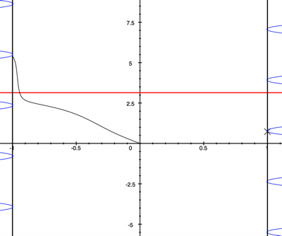
(a) $m=1,\quad\Psi(\eta),\eta\geq 0$

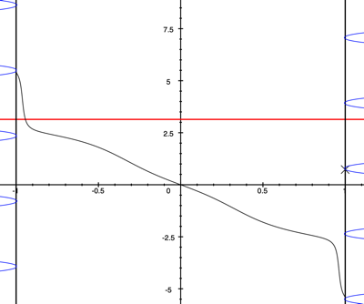
(b) $m=1,\quad\Psi(\eta),\eta\in\mathbb{R}$

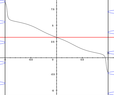
(c) $m=1,\quad\Psi(\eta)+(0,\pi),\eta\in\mathbb{R}$

(d) $m=5,\quad\Psi(\eta),\eta\geq 0$

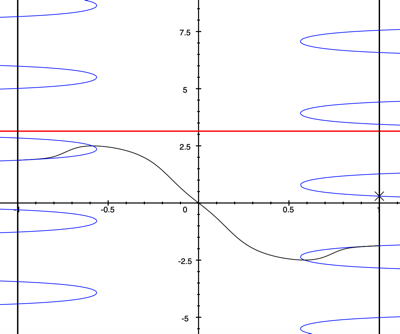
(e) $m=5,\quad\Psi(\eta),\eta\in\mathbb{R}$

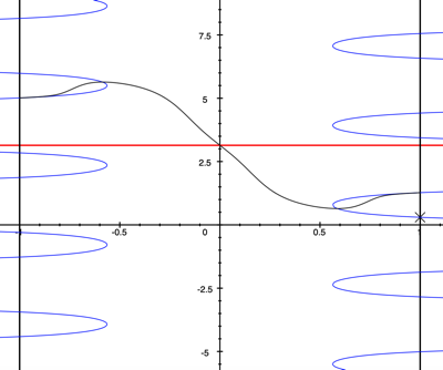
(f) $m=5,\quad\Psi(\eta)+(0,\pi),\eta\in\mathbb{R}$

Figure 4: In each figure above, the red horizontal line is $\theta=\pi$ and the blue curve is the level curve $2\sqrt{(2m+2)(2m+3)}z_{0}-\frac{n-1}{n}H\sin(\theta)\cos(\theta)=0$. The cross at $\{H=1\}$ is $A_{0}^{+}$. Plots above show that for $m=1$, the graph of $\Pi$ must be above $\Psi+(0,\pi)$ and hence $\theta_{*}>\pi$. On the other hand for $m=5$, the graph of $\Pi$ is below $\Psi+(0,\pi)$ and hence $\theta_{*}<\pi$.

Note that if $\Psi$ converges to $A_{1}^{-}$, then $\Pi=\Psi+(0,\pi)$ and we have $\theta_{*}=\pi$. In such a situation, a more delicate analysis is needed to obtain $\lim\limits_{s_{1}\to\infty}\sharp C(\gamma_{s_{1}})$ and $\lim\limits_{s_{2}\to\infty}\sharp C(\zeta_{s_{2}})$. In fact, Lemma 5.9 implies that as long as $\Psi$ does not converge to $A_{1}^{-}$ for a fixed $m$, we either have a second Einstein metric on $\mathbb{HP}^{m+1}\sharp\overline{\mathbb{HP}}^{m+1}$ or a new Einstein metric on $\mathbb{S}^{4m+4}$.

Fortunately, the 4th order Runge–Kutta algorithm shows that for $m\in[2,100]$, the integral curve $\Psi$ converges to $B_{1}^{-}$. Hence $\Pi$ must pass $(0,\theta_{*})$ for some $\theta_{*}<\pi$. Therefore, by Lemma 5.9, the second Einstein metric exists on $\mathbb{HP}^{m+1}\sharp\overline{\mathbb{HP}}^{m+1}$ for $m\in[2,100]$. The function $H$ in (5.7) can be solved explicitly. By Remark 2.4, it is clear that $H=-\tanh\left(\frac{2\eta}{n}\right).$ Hence the above discussion can be summarized into a more compact statement as in Theorem 1.2. Since $\Psi$ converges to one of the $O_{i}^{-}$’s, from (5.9) the inequality $\Omega<\frac{3\pi}{4}$ in Theorem 1.2 essentially means that $\Psi$ converges to $B_{1}^{-}$. As shown by the algorithm, for $m=1$ the integral curve $\Psi$ converges to $B_{2}^{-}$, meaning that $\Pi$ must pass $(0,\theta_{*})$ for some $\theta_{*}>\pi$. We show some plots of $\Psi$ for different $m$ on the $H\theta$-plane in Figure 5, generated by the 4th order Runge–Kutta algorithm with step size 0.01 in Grapher.

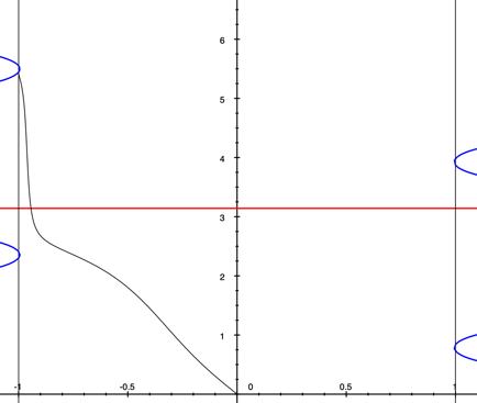
(a) $m=1$

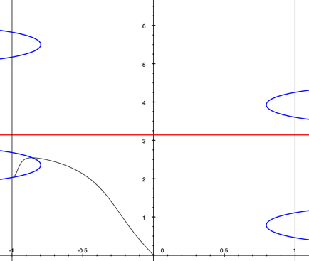
(b) $m=2$

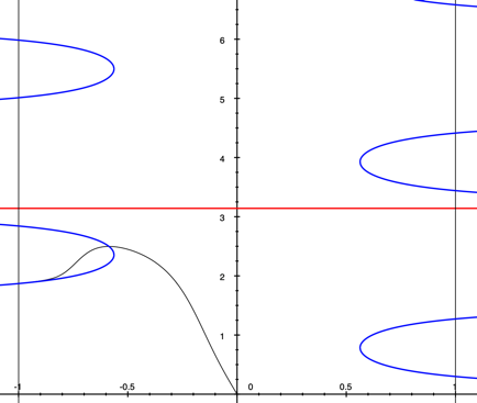
(c) $m=5$

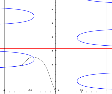
(d) $m=10$

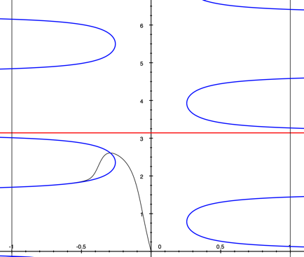
(e) $m=29$

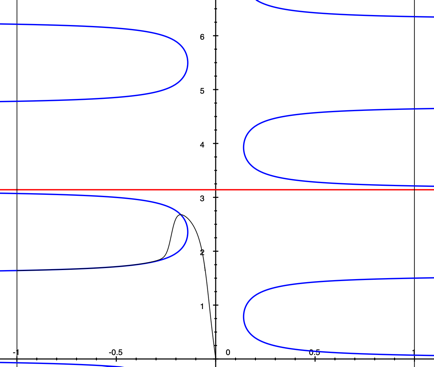
(f) $m=100$

Figure 5:

In the following lemma, we prove that $\Omega>\pi$ for $m=1$. Therefore, the inequality $\theta_{*}>\pi$ is indeed valid for $m=1$.

Lemma 5.10.

Let $\Psi$ be an integral curve to the following dynamical system

$$\begin{bmatrix}H\\ \theta\end{bmatrix}^{\prime}=\tilde{V}(H,\theta):=\begin{bmatrix}(H^{2}-1)\frac{1}{7}\\ \frac{4\sqrt{5}}{21}-\frac{3}{7}H\sin(2\theta)\end{bmatrix}$$ (5.11)

with $\Psi(0)=(0,0)$. Then $\lim\limits_{\eta\to\infty}\theta(\Psi)>\pi$.

Proof.

Let $H_{1}=\frac{2}{e^{\frac{\sqrt{5}\pi}{6}}+1}-1\approx-0.527$ and $H_{2}=\frac{2}{\pi-2-2a_{1}^{-}}\approx-0.543$. Define the following function.

$$\Theta(H)=\left\{\begin{array}[]{ll}\frac{1}{H}+1+a_{1}^{-}&-1\leq H\leq H_{2}\\ \frac{\pi}{2}&H_{2}<H<H_{1}\\ \frac{3\sqrt{5}}{5}\ln\left(\frac{1-H}{1+H}\right)&H_{1}\leq H\leq 0\end{array}\right..$$

Recall in (5.8) we have $a_{1}^{-}=\pi-\arctan\left(\frac{2\sqrt{5}}{5}\right)$. Then we have

$$\sin(a_{1}^{-})=\frac{2}{3},\quad\cos(a_{1}^{-})=-\frac{\sqrt{5}}{3},\quad\sin(2a_{1}^{-})=-\frac{4\sqrt{5}}{9},\quad\cos(2a_{1}^{-})=\frac{1}{9}.$$

The function $\Theta$ is non-increasing. The numbers $H_{1}$ and $H_{2}$ are chosen so that $\{\theta-\Theta(H)=0\}$ is a continuous curve that joins the origin and $A_{1}^{-}$.

We show that $\tilde{V}$ restricted to $\{\theta-\Theta(H)=0\}$ points upward. For $(H,\theta)\in(H_{1},0)\times\left(0,\frac{\pi}{2}\right)$, we have

$$\begin{split}\left\langle\nabla\left(\theta-\frac{3\sqrt{5}}{5}\ln\left(\frac{1-H}{1+H}\right)\right),\tilde{V}\right\rangle&=\frac{4\sqrt{5}}{21}-\frac{3}{7}H\sin(2\theta)+\frac{6\sqrt{5}}{5}\frac{1}{1-H^{2}}\frac{H^{2}-1}{7}\\ &=\frac{2\sqrt{5}}{105}-\frac{3}{7}H\sin(2\theta)\\ &>0.\end{split}$$ (5.12)

Therefore, the function $\theta-\Theta(H)$ remains positive along $\Psi$ as $H$ decreases from $0$ to $H_{1}$. The computation above also shows that the function $\theta-\Theta(H)$ is positive along $\Psi(\eta)$ once the integral curve leaves the origin. If $\theta=\frac{\pi}{2}$, then $\left\langle\nabla\theta,\tilde{V}\right\rangle=\frac{4\sqrt{5}}{21}>0.$ Hence $\theta>\frac{\pi}{2}$ along $\Psi$ as $H$ decreases from $H_{1}$ to $H_{2}$.

Finally, as $H$ decreases from $H_{2}$ to $-1$, the function $\Theta(H)$ increases from $\frac{\pi}{2}$ to $a_{1}^{-}$. We first claim that for $\theta\in\left[\frac{\pi}{2},a_{1}^{-}\right]$, the inequality

$$D(\theta):=\sin(2\theta)-\left(\theta-\frac{\pi}{2}\right)\left(\frac{7}{4}(\theta-a_{1}^{-})+\frac{\sin(2a_{1}^{-})}{a_{1}^{-}-\frac{\pi}{2}}\right)\geq 0$$ (5.13)

is valid. It is obvious that $D(a_{1}^{-})=D\left(\frac{\pi}{2}\right)=0$. Hence there exists some $\theta_{1}\in\left(\frac{\pi}{2},a_{1}^{-}\right)$ that $D^{\prime}(\theta_{1})=0$ by the mean value theorem. On the other hand, we have

$$D^{\prime}(\theta)=2\cos(2\theta)-\left(\frac{7}{4}(\theta-a_{1}^{-})+\frac{\sin(2a_{1}^{-})}{a_{1}^{-}-\frac{\pi}{2}}\right)-\frac{7}{4}\left(\theta-\frac{\pi}{2}\right),\quad D^{\prime\prime}(\theta)=-4\sin(2\theta)-\frac{7}{2}.$$

Hence $D^{\prime\prime}>0$ on $\left(\frac{\pi}{2}+\frac{1}{2}\arcsin\left(\frac{7}{8}\right),\pi-\frac{1}{2}\arcsin\left(\frac{7}{8}\right)\right)$. Since $\pi-\frac{1}{2}\arcsin\left(\frac{7}{8}\right)\approx 2.609>2.412\approx a_{1}^{-}$, it is clear that $D^{\prime}$ decreases in $\left(\frac{\pi}{2},\frac{\pi}{2}+\frac{1}{2}\arcsin\left(\frac{7}{8}\right)\right)$ and increases in $\left(\frac{\pi}{2}+\frac{1}{2}\arcsin\left(\frac{7}{8}\right),a_{1}^{-}\right)$. Since

$$\begin{split}&D^{\prime}\left(\frac{\pi}{2}\right)=-2-\left(\frac{7}{4}\left(\frac{\pi}{2}-a_{1}^{-}\right)+\frac{\sin(2a_{1}^{-})}{a_{1}^{-}-\frac{\pi}{2}}\right)\approx 0.654>0,\\ &D^{\prime}\left(a_{1}^{-}\right)=2\cos(2a_{1}^{-})-\frac{\sin(2a_{1}^{-})}{a_{1}^{-}-\frac{\pi}{2}}-\frac{7}{4}\left(a_{1}^{-}-\frac{\pi}{2}\right)\approx-0.068<0,\end{split}$$ (5.14)

we know that $D^{\prime}$ only vanishes once in $\left[\frac{\pi}{2},a_{1}^{-}\right]$. Therefore, the function $D$ is indeed positive for $\theta\in\left(\frac{\pi}{2},a_{1}^{-}\right)$.

Then from (5.13) we have

$$\begin{split}&\left.\left\langle\nabla\left(\theta-\frac{1}{H}-1-a_{1}^{-}\right),\tilde{V}\right\rangle\right|_{\theta-\frac{1}{H}-1-a_{1}^{-}=0}\\ &=\frac{4\sqrt{5}}{21}-\frac{3}{7}H\sin(2\theta)+\frac{1}{7H^{2}}(H^{2}-1)\\ &\geq\frac{4\sqrt{5}}{21}-\frac{3}{7}H\left(\theta-\frac{\pi}{2}\right)\left(\frac{7}{4}(\theta-a_{1}^{-})+\frac{\sin(2a_{1}^{-})}{a_{1}^{-}-\frac{\pi}{2}}\right)+\frac{1}{7H^{2}}(H^{2}-1)\\ &=\frac{4\sqrt{5}}{21}-\frac{3}{7}H\left(\frac{1+H}{H}+a_{1}^{-}-\frac{\pi}{2}\right)\left(\frac{7}{4}\left(\frac{1+H}{H}\right)+\frac{\sin(2a_{1}^{-})}{a_{1}^{-}-\frac{\pi}{2}}\right)+\frac{1}{7H^{2}}(H^{2}-1)\\ &\quad\text{since $\theta-\frac{1}{H}-1-a_{1}^{-}=0$}\\ &=\frac{4\sqrt{5}}{21}(1+H)-\left(\frac{3}{4}\left(a_{1}^{-}-\frac{\pi}{2}\right)+\frac{3}{7}\frac{\sin(2a_{1}^{-})}{a_{1}^{-}-\frac{\pi}{2}}\right)(1+H)-\frac{3}{4}\frac{(1+H)^{2}}{H}+\frac{1}{7H^{2}}(H^{2}-1).\end{split}$$ (5.15)

Since $\frac{4\sqrt{5}}{21}-\left(\frac{3}{4}\left(a_{1}^{-}-\frac{\pi}{2}\right)+\frac{3}{7}\frac{\sin(2a_{1}^{-})}{a_{1}^{-}-\frac{\pi}{2}}\right)\approx 0.3015>0.3$, the computation above continues as

$$\begin{split}\left.\left\langle\nabla\left(\theta-\frac{1}{H}-1-a_{1}^{-}\right),\tilde{V}\right\rangle\right|_{\theta-\frac{1}{H}-1-a_{1}^{-}=0}&\geq\frac{3}{10}(1+H)-\frac{3}{4}\frac{(1+H)^{2}}{H}+\frac{1}{7H^{2}}(H^{2}-1)\\ &=\frac{1+H}{H^{2}}\left(-\frac{9}{20}H^{2}-\frac{17}{28}H-\frac{1}{7}\right).\end{split}$$ (5.16)

A straightforward computation shows that the factor $-\frac{9}{20}H^{2}-\frac{17}{28}H-\frac{1}{7}$ is positive on $\left[-1,-\frac{1}{2}\right]$. As $H_{2}<-\frac{1}{2}$, it is proved that $\Psi$ does not pass the barrier $\theta-\Theta(H)=0$ where $H\in(-1,H_{2})$. Therefore, we must have $\lim\limits_{\eta\to\infty}\theta(\Psi)\geq a_{1}^{-}$.

We claim that $\Psi$ does not converge to $A_{1}^{-}$. The linearization of (5.11) at $A_{1}^{-}$ is $\begin{bmatrix}-\frac{2}{7}&0\\ \frac{4\sqrt{5}}{21}&\frac{2}{21}\end{bmatrix}$, whose only stable eigenvalue and eigenvector are respectively $-\frac{2}{7}$ and $\begin{bmatrix}2\\ -\sqrt{5}\\ \end{bmatrix}$. Hence the linearized solution in $\{H>-1\}$ takes the form of $A_{1}^{-}+\begin{bmatrix}2\\ -\sqrt{5}\\ \end{bmatrix}e^{-\frac{2}{7}\eta}$. Suppose $\Psi$ is the integral curve that tends to $A_{1}^{-}$. We must have

$$(\theta-\Theta(H))(\Psi(\eta))\sim(\theta-\Theta(H))\left(A_{1}^{-}+\begin{bmatrix}2\\ -\sqrt{5}\\ \end{bmatrix}e^{-\frac{2}{7}\eta}\right)=-e^{-\frac{2}{7}\eta}\left(\sqrt{5}-\frac{2}{1-2e^{-\frac{2}{7}\eta}}\right)<0$$

as $\eta\to\infty$, which is a contradiction. Therefore, the integral curve $\Psi$ converges to some $O_{i}^{-}$ with $i\geq 2$. As $A_{2}^{-}>B_{2}^{-}>\pi$, we conclude that $\lim\limits_{\eta\to\infty}\theta(\Psi)>\pi$. ∎

Theorem 1.3 is proved with Lemma 5.10 established.

6 Appendix

6.1 Detailed computation of (4.18) and (4.20)

We first give detailed computation for $\left\langle\nabla A,V\right\rangle$ in the following.

$$\begin{split}&\left\langle\nabla A,V\right\rangle\\ &=Y\left(X_{2}H\left(G+\frac{1}{n}(1-H^{2})-1\right)+R_{2}-\frac{1}{n}(1-H^{2})\right)+YX_{2}\left(H\left(G+\frac{1}{n}(1-H^{2})\right)-X_{1}\right)\\ &\quad-\frac{3}{m}Z\left(\left(X_{1}+\frac{2m}{3}X_{2}\right)H\left(G+\frac{1}{n}(1-H^{2})-1\right)+R_{1}+\frac{2m}{3}R_{2}-\left(1+\frac{2m}{3}\right)\frac{1}{n}(1-H^{2})\right)\\ &\quad-\frac{3}{m}Z\left(X_{1}+\frac{2m}{3}X_{2}\right)\left(H\left(G+\frac{1}{n}(1-H^{2})\right)+X_{1}-2X_{2}\right)\\ &=Y\left(2X_{2}H\left(G+\frac{1}{n}(1-H^{2})\right)-X_{2}H+R_{2}-\frac{1}{n}(1-H^{2})\right)+YX_{2}\left(-X_{1}\right)\\ &\quad-\frac{3}{m}Z\left(2\left(X_{1}+\frac{2m}{3}X_{2}\right)H\left(G+\frac{1}{n}(1-H^{2})\right)-\left(X_{1}+\frac{2m}{3}X_{2}\right)H+R_{1}+\frac{2m}{3}R_{2}-\left(1+\frac{2m}{3}\right)\frac{1}{n}(1-H^{2})\right)\\ &\quad-\frac{3}{m}Z\left(X_{1}+\frac{2m}{3}X_{2}\right)(X_{1}-2X_{2})\\ &=2YX_{2}H\left(G+\frac{1}{n}(1-H^{2})\right)+Y\left(-X_{2}H+R_{2}-\frac{1}{n}(1-H^{2})\right)+YX_{2}\left(-X_{1}\right)\\ &\quad-2\frac{3}{m}Z\left(X_{1}+\frac{2m}{3}X_{2}\right)H\left(G+\frac{1}{n}(1-H^{2})\right)\\ &\quad-\frac{3}{m}Z\left(-\left(X_{1}+\frac{2m}{3}X_{2}\right)H+R_{1}+\frac{2m}{3}R_{2}-\left(1+\frac{2m}{3}\right)\frac{1}{n}(1-H^{2})\right)\\ &\quad-\frac{3}{m}Z\left(X_{1}+\frac{2m}{3}X_{2}\right)(X_{1}-2X_{2})\\ &=2AH\left(G+\frac{1}{n}(1-H^{2})\right)+Y\left(-X_{2}H+R_{2}-\frac{1}{n}(1-H^{2})\right)+YX_{2}\left(-X_{1}\right)\\ &\quad-\frac{3}{m}Z\left(-\left(X_{1}+\frac{2m}{3}X_{2}\right)H+R_{1}+\frac{2m}{3}R_{2}-\left(1+\frac{2m}{3}\right)\frac{1}{n}(1-H^{2})\right)\\ &\quad-\frac{3}{m}Z\left(X_{1}+\frac{2m}{3}X_{2}\right)(X_{1}-2X_{2})\\ &=2AH\left(G+\frac{1}{n}(1-H^{2})\right)+Y\left(-X_{2}(2X_{1}+(4m+2)X_{2})-X_{2}(2X_{1}-2X_{2})+R_{2}-\frac{1}{n}(1-H^{2})\right)\\ &\quad-\frac{3}{m}Z\left(-\left(X_{1}+\frac{2m}{3}X_{2}\right)(2X_{1}+(4m+2)X_{2})+R_{1}+\frac{2m}{3}R_{2}-\left(1+\frac{2m}{3}\right)\frac{1}{n}(1-H^{2})\right)\\ &=2AH\left(G+\frac{1}{n}(1-H^{2})\right)-YX_{2}(2X_{1}+(4m+2)X_{2})+Y\left(-X_{2}(2X_{1}-2X_{2})+R_{2}-\frac{1}{n}(1-H^{2})\right)\\ &\quad+\frac{3}{m}Z\left(X_{1}+\frac{2m}{3}X_{2}\right)(2X_{1}+(4m+2)X_{2})-\frac{3}{m}Z\left(R_{1}+\frac{2m}{3}R_{2}-\left(1+\frac{2m}{3}\right)\frac{1}{n}(1-H^{2})\right)\\ &=A\left(2H\left(G+\frac{1}{n}(1-H^{2})\right)-(2X_{1}+(4m+2)X_{2})\right)\\ &\quad+Y\left(-X_{2}(2X_{1}-2X_{2})+R_{2}-\frac{1}{n}(1-H^{2})\right)-\frac{3}{m}Z\left(R_{1}+\frac{2m}{3}R_{2}-\left(1+\frac{2m}{3}\right)\frac{1}{n}(1-H^{2})\right).\end{split}$$ (6.1)

The last two terms in the computation above continue as the following.

$$\begin{split}&Y\left(-X_{2}(2X_{1}-2X_{2})+R_{2}-\frac{1}{n}(1-H^{2})\right)-\frac{3}{m}Z\left(R_{1}+\frac{2m}{3}R_{2}-\left(1+\frac{2m}{3}\right)\frac{1}{n}(1-H^{2})\right)\\ &=Y\left(R_{2}-\frac{1}{n}(1-H^{2})\right)-2YX_{2}(X_{1}-X_{2})-\frac{3}{m}Z\left(R_{1}+\frac{2m}{3}R_{2}-\left(1+\frac{2m}{3}\right)\frac{1}{n}(1-H^{2})\right)\\ &=\frac{1}{X_{2}(X_{1}+\frac{2m}{3}X_{2})}\left(YX_{2}(X_{1}+\frac{2m}{3}X_{2})\left(R_{2}-\frac{1}{n}(1-H^{2})\right)\right)\\ &\quad-\frac{1}{X_{2}(X_{1}+\frac{2m}{3}X_{2})}\left(2YX_{2}^{2}(X_{1}-X_{2})\left(X_{1}+\frac{2m}{3}X_{2}\right)\right)\\ &\quad+\frac{1}{X_{2}(X_{1}+\frac{2m}{3}X_{2})}\left(-\frac{3}{m}ZX_{2}(X_{1}+\frac{2m}{3}X_{2})\left(R_{1}+\frac{2m}{3}R_{2}-\left(1+\frac{2m}{3}\right)\frac{1}{n}(1-H^{2})\right)\right)\\ &=\frac{1}{X_{2}(X_{1}+\frac{2m}{3}X_{2})}\left(YX_{2}(X_{1}+\frac{2m}{3}X_{2})\left(R_{2}-\frac{1}{n}(1-H^{2})\right)\right)\\ &\quad-\frac{1}{X_{2}(X_{1}+\frac{2m}{3}X_{2})}\left(2YX_{2}^{2}(X_{1}-X_{2})\left(X_{1}+\frac{2m}{3}X_{2}\right)\right)\\ &\quad+\frac{1}{X_{2}(X_{1}+\frac{2m}{3}X_{2})}\left((A-YX_{2})X_{2}\left(R_{1}+\frac{2m}{3}R_{2}-\left(1+\frac{2m}{3}\right)\frac{1}{n}(1-H^{2})\right)\right)\\ &=\frac{1}{X_{2}(X_{1}+\frac{2m}{3}X_{2})}\left(YX_{2}(X_{1}+\frac{2m}{3}X_{2})\left(R_{2}-\frac{1}{n}(1-H^{2})\right)\right)\\ &\quad-\frac{1}{X_{2}(X_{1}+\frac{2m}{3}X_{2})}\left(2YX_{2}^{2}(X_{1}-X_{2})\left(X_{1}+\frac{2m}{3}X_{2}\right)\right)\\ &\quad+\frac{1}{X_{2}(X_{1}+\frac{2m}{3}X_{2})}\left(-YX_{2}^{2}\left(R_{1}+\frac{2m}{3}R_{2}-\left(1+\frac{2m}{3}\right)\frac{1}{n}(1-H^{2})\right)\right)\\ &\quad+\frac{1}{X_{2}(X_{1}+\frac{2m}{3}X_{2})}\left(AX_{2}\left(R_{1}+\frac{2m}{3}R_{2}-\left(1+\frac{2m}{3}\right)\frac{1}{n}(1-H^{2})\right)\right)\\ &=\frac{Y}{X_{1}+\frac{2m}{3}X_{2}}(X_{1}+\frac{2m}{3}X_{2})\left(R_{2}-\frac{1}{n}(1-H^{2})\right)\\ &\quad-\frac{Y}{X_{1}+\frac{2m}{3}X_{2}}\left(2X_{2}(X_{1}-X_{2})\left(X_{1}+\frac{2m}{3}X_{2}\right)\right)\\ &\quad+\frac{Y}{X_{1}+\frac{2m}{3}X_{2}}\left(-X_{2}\left(R_{1}+\frac{2m}{3}R_{2}-\left(1+\frac{2m}{3}\right)\frac{1}{n}(1-H^{2})\right)\right)\\ &\quad+\frac{A}{X_{1}+\frac{2m}{3}X_{2}}\left(R_{1}+\frac{2m}{3}R_{2}-\left(1+\frac{2m}{3}\right)\frac{1}{n}(1-H^{2})\right)\\ &=\frac{Y}{X_{1}+\frac{2m}{3}X_{2}}\left((X_{1}+\frac{2m}{3}X_{2})\left(R_{2}-\frac{1}{n}(1-H^{2})\right)-X_{2}\left(R_{1}+\frac{2m}{3}R_{2}-\left(1+\frac{2m}{3}\right)\frac{1}{n}(1-H^{2})\right)\right)\\ &\quad-\frac{Y}{X_{1}+\frac{2m}{3}X_{2}}\left(2X_{2}(X_{1}-X_{2})\left(X_{1}+\frac{2m}{3}X_{2}\right)\right)\\ &\quad+\frac{A}{X_{1}+\frac{2m}{3}X_{2}}\left(R_{1}+\frac{2m}{3}R_{2}-\left(1+\frac{2m}{3}\right)\frac{1}{n}(1-H^{2})\right)\\ &=\frac{Y}{X_{1}+\frac{2m}{3}X_{2}}\left(X_{1}\left(R_{2}-\frac{1}{n}(1-H^{2})\right)-X_{2}\left(R_{1}-\frac{1}{n}(1-H^{2})\right)-2X_{2}(X_{1}-X_{2})\left(X_{1}+\frac{2m}{3}X_{2}\right)\right)\\ &\quad+\frac{A}{X_{1}+\frac{2m}{3}X_{2}}\left(R_{1}+\frac{2m}{3}R_{2}-\left(1+\frac{2m}{3}\right)\frac{1}{n}(1-H^{2})\right)\\ &=\frac{Y}{X_{1}+\frac{2m}{3}X_{2}}P+\frac{A}{X_{1}+\frac{2m}{3}X_{2}}\left(R_{1}+\frac{2m}{3}R_{2}-\left(1+\frac{2m}{3}\right)\frac{1}{n}(1-H^{2})\right).\end{split}$$ (6.2)

Hence computation (4.18) indeed holds.

We give detailed computation for $\langle\nabla P,V\rangle$ in the following. First of all, we have

$$\begin{split}&\left\langle\nabla\left(R_{1}-\frac{1}{n}(1-H^{2})\right),V\right\rangle\\ &=\left\langle\nabla\left(2Y^{2}+4mZ^{2}-\frac{1}{n}(1-H^{2})\right),V\right\rangle\\ &=4Y^{2}\left(H\left(G+\frac{1}{n}(1-H^{2})\right)-X_{1}\right)+8mZ^{2}\left(H\left(G+\frac{1}{n}(1-H^{2})\right)+X_{1}-2X_{2}\right)\\ &\quad+\frac{2H}{n}(H^{2}-1)\left(G+\frac{1}{n}(1-H^{2})\right)\\ &=2\left(R_{1}-\frac{1}{n}(1-H^{2})\right)H\left(G+\frac{1}{n}(1-H^{2})\right)-4Y^{2}X_{1}+8mZ^{2}(X_{1}-2X_{2})\\ &=2\left(R_{1}-\frac{1}{n}(1-H^{2})\right)H\left(G+\frac{1}{n}(1-H^{2})\right)-(4Y^{2}-8mZ^{2})(X_{1}-X_{2})-2R_{1}X_{2},\end{split}$$ (6.3)

and

$$\begin{split}&\left\langle\nabla\left(R_{2}-\frac{1}{n}(1-H^{2})\right),V\right\rangle\\ &=\left\langle\nabla\left((4m+8)YZ-6Z^{2}-\frac{1}{n}(1-H^{2})\right),V\right\rangle\\ &=2(4m+8)YZ\left(H\left(G+\frac{1}{n}(1-H^{2})\right)-X_{2}\right)-12Z^{2}\left(H\left(G+\frac{1}{n}(1-H^{2})\right)+X_{1}-2X_{2}\right)\\ &\quad+\frac{2H}{n}(H^{2}-1)\left(G+\frac{1}{n}(1-H^{2})\right)\\ &=2\left(R_{2}-\frac{1}{n}(1-H^{2})\right)H\left(G+\frac{1}{n}(1-H^{2})\right)-2(4m+8)YZX_{2}-12Z^{2}(X_{1}-2X_{2})\\ &=2\left(R_{2}-\frac{1}{n}(1-H^{2})\right)H\left(G+\frac{1}{n}(1-H^{2})\right)-((4m+8)YZ+6Z^{2})(X_{1}-X_{2})-R_{2}(3X_{2}-X_{1}).\end{split}$$ (6.4)

Then it follows that

$$\begin{split}&X_{1}\left\langle\nabla\left(R_{2}-\frac{1}{n}(1-H^{2})\right),V\right\rangle-X_{2}\left\langle\nabla\left(R_{1}-\frac{1}{n}(1-H^{2})\right),V\right\rangle\\ &=2X_{1}\left(R_{2}-\frac{1}{n}(1-H^{2})\right)H\left(G+\frac{1}{n}(1-H^{2})\right)-((4m+8)YZ+6Z^{2})X_{1}(X_{1}-X_{2})-R_{2}X_{1}(3X_{2}-X_{1})\\ &\quad-2X_{2}\left(R_{1}-\frac{1}{n}(1-H^{2})\right)H\left(G+\frac{1}{n}(1-H^{2})\right)+(4Y^{2}-8mZ^{2})X_{2}(X_{1}-X_{2})+2R_{1}X_{2}^{2}\\ &=2X_{1}\left(R_{2}-\frac{1}{n}(1-H^{2})\right)H\left(G+\frac{1}{n}(1-H^{2})\right)-((4m+8)YZ+6Z^{2})X_{1}(X_{1}-X_{2})-R_{2}X_{1}(3X_{2}-X_{1})\\ &\quad-2X_{2}\left(R_{1}-\frac{1}{n}(1-H^{2})\right)H\left(G+\frac{1}{n}(1-H^{2})\right)+(4Y^{2}-8mZ^{2})X_{2}(X_{1}-X_{2})+2R_{1}X_{2}^{2}\\ &\quad-4X_{2}\left(X_{1}+\frac{2m}{3}X_{2}\right)(X_{1}-X_{2})H\left(G+\frac{1}{n}(1-H^{2})\right)\\ &\quad+4X_{2}\left(X_{1}+\frac{2m}{3}X_{2}\right)(X_{1}-X_{2})H\left(G+\frac{1}{n}(1-H^{2})\right)\\ &=2PH\left(G+\frac{1}{n}(1-H^{2})\right)\\ &\quad-((4m+8)YZ+6Z^{2})X_{1}(X_{1}-X_{2})-R_{2}X_{1}(3X_{2}-X_{1})+(4Y^{2}-8mZ^{2})X_{2}(X_{1}-X_{2})+2R_{1}X_{2}^{2}\\ &\quad+4X_{2}\left(X_{1}+\frac{2m}{3}X_{2}\right)(X_{1}-X_{2})H\left(G+\frac{1}{n}(1-H^{2})\right)\\ &=2PH\left(G+\frac{1}{n}(1-H^{2})\right)\\ &\quad+(X_{1}-X_{2})\left((4Y^{2}-8mZ^{2})X_{2}-((4m+8)YZ+6Z^{2})X_{1}\right)-R_{2}X_{1}(3X_{2}-X_{1})+2R_{1}X_{2}^{2}\\ &\quad+4X_{2}\left(X_{1}+\frac{2m}{3}X_{2}\right)(X_{1}-X_{2})H\left(G+\frac{1}{n}(1-H^{2})\right).\end{split}$$ (6.5)

Then we have

$$\begin{split}&\langle\nabla P,V\rangle\\ &=\left\langle\nabla\left(X_{1}\left(R_{2}-\frac{1}{n}(1-H^{2})\right)-X_{2}\left(R_{1}-\frac{1}{n}(1-H^{2})\right)-2X_{2}\left(X_{1}+\frac{2m}{3}X_{2}\right)(X_{1}-X_{2})\right),V\right\rangle\\ &=\left(X_{1}H\left(G+\frac{1}{n}(1-H^{2})-1\right)+R_{1}-\frac{1}{n}(1-H^{2})\right)\left(R_{2}-\frac{1}{n}(1-H^{2})\right)+X_{1}\left\langle\nabla\left(R_{2}-\frac{1}{n}(1-H^{2})\right),V\right\rangle\\ &\quad-\left(X_{2}H\left(G+\frac{1}{n}(1-H^{2})-1\right)+R_{2}-\frac{1}{n}(1-H^{2})\right)\left(R_{1}-\frac{1}{n}(1-H^{2})\right)-X_{2}\left\langle\nabla\left(R_{1}-\frac{1}{n}(1-H^{2})\right),V\right\rangle\\ &\quad-2\left(X_{1}+\frac{2m}{3}X_{2}\right)(X_{1}-X_{2})\left(X_{2}H\left(G+\frac{1}{n}(1-H^{2})-1\right)+R_{2}-\frac{1}{n}(1-H^{2})\right)\\ &\quad-2X_{2}(X_{1}-X_{2})\left(\left(X_{1}+\frac{2m}{3}X_{2}\right)H\left(G+\frac{1}{n}(1-H^{2})-1\right)+R_{1}+\frac{2m}{3}R_{2}-\left(1+\frac{2m}{3}\right)\frac{1}{n}(1-H^{2})\right)\\ &\quad-2X_{2}\left(X_{1}+\frac{2m}{3}X_{2}\right)\left((X_{1}-X_{2})H\left(G+\frac{1}{n}(1-H^{2})-1\right)+R_{1}-R_{2}\right)\\ &=X_{1}\left(R_{2}-\frac{1}{n}(1-H^{2})\right)H\left(G+\frac{1}{n}(1-H^{2})-1\right)+X_{1}\left\langle\nabla\left(R_{2}-\frac{1}{n}(1-H^{2})\right),V\right\rangle\\ &\quad-X_{2}\left(R_{1}-\frac{1}{n}(1-H^{2})\right)H\left(G+\frac{1}{n}(1-H^{2})-1\right)-X_{2}\left\langle\nabla\left(R_{1}-\frac{1}{n}(1-H^{2})\right),V\right\rangle\\ &\quad-2\left(X_{1}+\frac{2m}{3}X_{2}\right)(X_{1}-X_{2})X_{2}H\left(G+\frac{1}{n}(1-H^{2})-1\right)-2\left(X_{1}+\frac{2m}{3}X_{2}\right)(X_{1}-X_{2})\left(R_{2}-\frac{1}{n}(1-H^{2})\right)\\ &\quad-2X_{2}(X_{1}-X_{2})\left(\left(X_{1}+\frac{2m}{3}X_{2}\right)H\left(G+\frac{1}{n}(1-H^{2})-1\right)+R_{1}+\frac{2m}{3}R_{2}-\left(1+\frac{2m}{3}\right)\frac{1}{n}(1-H^{2})\right)\\ &\quad-2X_{2}\left(X_{1}+\frac{2m}{3}X_{2}\right)\left((X_{1}-X_{2})H\left(G+\frac{1}{n}(1-H^{2})-1\right)+R_{1}-R_{2}\right)\\ &=PH\left(G+\frac{1}{n}(1-H^{2})-1\right)\\ &\quad+X_{1}\left\langle\nabla\left(R_{2}-\frac{1}{n}(1-H^{2})\right),V\right\rangle-X_{2}\left\langle\nabla\left(R_{1}-\frac{1}{n}(1-H^{2})\right),V\right\rangle\\ &\quad-2\left(X_{1}+\frac{2m}{3}X_{2}\right)(X_{1}-X_{2})\left(R_{2}-\frac{1}{n}(1-H^{2})\right)\\ &\quad-4X_{2}(X_{1}-X_{2})\left(X_{1}+\frac{2m}{3}X_{2}\right)H\left(G+\frac{1}{n}(1-H^{2})-1\right)\\ &\quad-2X_{2}(X_{1}-X_{2})\left(R_{1}+\frac{2m}{3}R_{2}-\left(1+\frac{2m}{3}\right)\frac{1}{n}(1-H^{2})\right)-2X_{2}\left(X_{1}+\frac{2m}{3}X_{2}\right)(R_{1}-R_{2}).\end{split}$$ (6.6)

The first term in the last line of the computation above is obtained by gathering the first, the third, and the fifth term from the second last line. From (6.5), the computation above continues as the following.

$$\begin{split}&=PH\left(G+\frac{1}{n}(1-H^{2})-1\right)\\ &\quad+2PH\left(G+\frac{1}{n}(1-H^{2})\right)\\ &\quad+(X_{1}-X_{2})\left((4Y^{2}-8mZ^{2})X_{2}-((4m+8)YZ+6Z^{2})X_{1}\right)-R_{2}X_{1}(3X_{2}-X_{1})+2R_{1}X_{2}^{2}\\ &\quad+4X_{2}\left(X_{1}+\frac{2m}{3}X_{2}\right)(X_{1}-X_{2})H\left(G+\frac{1}{n}(1-H^{2})\right)\\ &\quad-2\left(X_{1}+\frac{2m}{3}X_{2}\right)(X_{1}-X_{2})\left(R_{2}-\frac{1}{n}(1-H^{2})\right)\\ &\quad-4X_{2}(X_{1}-X_{2})\left(X_{1}+\frac{2m}{3}X_{2}\right)H\left(G+\frac{1}{n}(1-H^{2})-1\right)\\ &\quad-2X_{2}(X_{1}-X_{2})\left(R_{1}+\frac{2m}{3}R_{2}-\left(1+\frac{2m}{3}\right)\frac{1}{n}(1-H^{2})\right)-2X_{2}\left(X_{1}+\frac{2m}{3}X_{2}\right)(R_{1}-R_{2})\\ &=PH\left(3G+\frac{3}{n}(1-H^{2})-1\right)\\ &\quad+(X_{1}-X_{2})\left((4Y^{2}-8mZ^{2})X_{2}-((4m+8)YZ+6Z^{2})X_{1}\right)-R_{2}X_{1}(3X_{2}-X_{1})+2R_{1}X_{2}^{2}\\ &\quad-2(X_{1}-X_{2})\left(X_{1}+\frac{2m}{3}X_{2}\right)\left(R_{2}-\frac{1}{n}(1-H^{2})\right)\\ &\quad+4X_{2}(X_{1}-X_{2})\left(X_{1}+\frac{2m}{3}X_{2}\right)H\\ &\quad-2X_{2}(X_{1}-X_{2})\left(R_{1}+\frac{2m}{3}R_{2}-\left(1+\frac{2m}{3}\right)\frac{1}{n}(1-H^{2})\right)-2X_{2}\left(X_{1}+\frac{2m}{3}X_{2}\right)(R_{1}-R_{2})\\ &=PH\left(3G+\frac{3}{n}(1-H^{2})-1\right)\\ &\quad+(X_{1}-X_{2})\left((4Y^{2}-8mZ^{2})X_{2}-((4m+8)YZ+6Z^{2})X_{1}\right)\\ &\quad-2(X_{1}-X_{2})\left(X_{1}+\frac{2m}{3}X_{2}\right)\left(R_{2}-\frac{1}{n}(1-H^{2})\right)\\ &\quad+4X_{2}(X_{1}-X_{2})\left(X_{1}+\frac{2m}{3}X_{2}\right)H\\ &\quad-2X_{2}(X_{1}-X_{2})\left(R_{1}+\frac{2m}{3}R_{2}-\left(1+\frac{2m}{3}\right)\frac{1}{n}(1-H^{2})\right)\\ &\quad+R_{2}X_{1}(X_{1}-X_{2})+2R_{1}X_{2}(X_{2}-X_{1})+\frac{4m}{3}X_{2}(X_{2}R_{2}-X_{2}R_{1})\\ &=PH\left(3G+\frac{3}{n}(1-H^{2})-1\right)\\ &\quad+(X_{1}-X_{2})\left((4Y^{2}-8mZ^{2})X_{2}-((4m+8)YZ+6Z^{2})X_{1}\right)\\ &\quad-2(X_{1}-X_{2})\left(X_{1}+\frac{2m}{3}X_{2}\right)\left(R_{2}-\frac{1}{n}(1-H^{2})\right)\\ &\quad+4X_{2}(X_{1}-X_{2})\left(X_{1}+\frac{2m}{3}X_{2}\right)H\\ &\quad-2X_{2}(X_{1}-X_{2})\left(R_{1}+\frac{2m}{3}R_{2}-\left(1+\frac{2m}{3}\right)\frac{1}{n}(1-H^{2})\right)\\ &\quad+R_{2}X_{1}(X_{1}-X_{2})+2R_{1}X_{2}(X_{2}-X_{1})+\frac{4m}{3}X_{2}R_{2}(X_{2}-X_{1})+\frac{4m}{3}X_{2}(X_{1}R_{2}-X_{2}R_{1}).\end{split}$$ (6.7)

Write the last term as

$$\begin{split}&\frac{4m}{3}X_{2}(X_{1}R_{2}-X_{2}R_{1})\\ &=\frac{4m}{3}X_{2}\left(X_{1}\left(R_{2}-\frac{1}{n}(1-H^{2})\right)-X_{2}\left(R_{1}-\frac{1}{n}(1-H^{2})\right)-2X_{2}\left(X_{1}+\frac{2m}{3}X_{2}\right)(X_{1}-X_{2})\right)\\ &\quad+\frac{4m}{3}X_{2}\left((X_{1}-X_{2})\frac{1}{n}(1-H^{2})+2X_{2}\left(X_{1}+\frac{2m}{3}X_{2}\right)(X_{1}-X_{2})\right)\\ &=\frac{4m}{3}PX_{2}+\frac{4m}{3}(X_{1}-X_{2})X_{2}\left(\frac{1}{n}(1-H^{2})+2X_{2}\left(X_{1}+\frac{2m}{3}X_{2}\right)\right).\end{split}$$ (6.8)

Then (6.7) continues as

$$\begin{split}&=PH\left(3G+\frac{3}{n}(1-H^{2})-1\right)\\ &\quad+(X_{1}-X_{2})\left((4Y^{2}-8mZ^{2})X_{2}-((4m+8)YZ+6Z^{2})X_{1}\right)\\ &\quad-2(X_{1}-X_{2})\left(X_{1}+\frac{2m}{3}X_{2}\right)\left(R_{2}-\frac{1}{n}(1-H^{2})\right)\\ &\quad+4X_{2}(X_{1}-X_{2})\left(X_{1}+\frac{2m}{3}X_{2}\right)H\\ &\quad-2X_{2}(X_{1}-X_{2})\left(R_{1}+\frac{2m}{3}R_{2}-\left(1+\frac{2m}{3}\right)\frac{1}{n}(1-H^{2})\right)\\ &\quad+R_{2}X_{1}(X_{1}-X_{2})+2R_{1}X_{2}(X_{2}-X_{1})+\frac{4m}{3}X_{2}R_{2}(X_{2}-X_{1})\\ &\quad+\frac{4m}{3}PX_{2}+\frac{4m}{3}(X_{1}-X_{2})X_{2}\left(\frac{1}{n}(1-H^{2})+2X_{2}\left(X_{1}+\frac{2m}{3}X_{2}\right)\right)\\ &=P\left(H\left(3G+\frac{3}{n}(1-H^{2})-1\right)+\frac{4m}{3}X_{2}\right)+(X_{1}-X_{2})Q.\end{split}$$ (6.9)

6.2 Coefficients for $\tilde{B}_{m,\kappa}$ and $\tilde{Q}_{m,\kappa}$

We list coefficients for $\tilde{B}_{m,\kappa}$ and $\tilde{Q}_{m,\kappa}$ in the following.

• $\tilde{B}_{m,\kappa}(x)=b_{2}x^{2}+b_{1}x+b_{0}$
  

  $$\begin{split}b_{2}&=-\frac{(96\kappa^{3}m^{3}+264\kappa^{2}m^{2}+216\kappa m+54)}{(1-\kappa)(2\kappa^{2}m(8m-5)+6\kappa(4m-1)+9)}<0,\\ b_{1}&=\frac{4(m+2)(4\kappa m+3)(2\kappa^{2}m+4\kappa m+3)}{(1-\kappa)(2\kappa^{2}m(8m-5)+6\kappa(4m-1)+9)}-\frac{2(4m+3)^{2}(2m+3)(m-1)}{m(2m+1)(8m+3)},\\ b_{0}&=-\frac{3(4+(4m-2)\kappa)(4\kappa m+3)\kappa}{(1-\kappa)(2\kappa^{2}m(8m-5)+6\kappa(4m-1)+9)}<0.\end{split}$$ (6.10)

• $\tilde{Q}_{m,\kappa}(x)=q_{2}x^{2}+q_{1}x+q_{0}$
  

  $$\begin{split}q_{2}&=-\frac{4(2\kappa m+3)(32\kappa^{3}m^{3}+\kappa^{2}m^{2}(96-68\kappa)+\kappa m(90-84\kappa)+27(1-\kappa))}{3(1-\kappa)(2\kappa^{2}m(8m-5)+6\kappa(4m-1)+9)}<0,\\ q_{1}&=\frac{16\kappa(m+2)(16\kappa^{3}m^{3}-18\kappa^{3}m^{2}+32\kappa^{2}m^{2}-24\kappa^{2}m+27\kappa m-9\kappa+9)}{3(1-\kappa)(2\kappa^{2}m(8m-5)+6\kappa(4m-1)+9)}>0,\\ q_{0}&=-\frac{4\kappa^{2}(32\kappa^{2}m^{3}-20\kappa^{2}m^{2}-6\kappa^{2}m+48\kappa m^{2}-6\kappa m-9\kappa+18m+9)}{3(1-\kappa)(2\kappa^{2}m(8m-5)+6\kappa(4m-1)+9)}<0.\end{split}$$ (6.11)

Proposition 6.1.

For any $(m,\kappa)\in[1,\infty)\times(0,1)$, the function $\tilde{B}_{m,\kappa}$ has a real root $\sigma(m,\kappa)$ in the interval $\left(0,\frac{m\kappa}{3+2m\kappa}\right)$. For $m=1$, polynomials $\tilde{B}_{1,\kappa}$ and $\tilde{Q}_{1,\kappa}$ share a common real root $\sigma(1,\kappa)=\frac{\kappa}{3+2\kappa}$.

Proof.

From (6.10), computations show that

$$\begin{split}\tilde{B}_{m,\kappa}(0)&=b_{0}<0,\\ \tilde{B}_{m,\kappa}\left(\frac{m\kappa}{3+2m\kappa}\right)&=\frac{768(m-1)\kappa B_{*}}{(8m+3)(2\kappa m+3)(2m+1)(1-\kappa)(2\kappa^{2}m(8m-5)+6\kappa(4m-1)+9)}\end{split}$$ (6.12)

where

$$\begin{split}B_{*}&=\left(m^{4}+\frac{15}{8}m^{3}+\frac{5}{16}m^{2}-\frac{45}{32}m-\frac{45}{64}\right)m\kappa^{3}\\ &\quad+\left(\frac{13}{4}m^{4}+\frac{163}{32}m^{3}+\frac{255}{64}m^{2}+\frac{9}{16}m-\frac{27}{64}\right)\kappa^{2}\\ &\quad+\left(\frac{21}{8}m^{3}+\frac{147}{64}m^{2}+\frac{243}{128}m+\frac{27}{32}\right)\kappa\\ &\quad+\frac{21}{32}m^{2}-\frac{27}{128}\\ &>0\end{split}$$ (6.13)

for any $(m,\kappa)\in[1,\infty)\times(0,1)$. Hence such a $\sigma(m,\kappa)$ exists. Furthermore, we have

$$\begin{split}\tilde{B}_{1,\kappa}(x)&=\frac{2(3+4\kappa)((2\kappa+1)x-\kappa-2)((2\kappa+3)x-\kappa)}{(2\kappa^{2}+6\kappa+3)(\kappa-1)},\\ \tilde{Q}_{1,\kappa}(x)&=-\frac{4((12\kappa^{3}-4\kappa^{2}-21\kappa-9)x+2\kappa^{3}+11\kappa^{2}+9\kappa)((2\kappa+3)x-\kappa)}{3(2\kappa^{2}+6\kappa+3)(\kappa-1)}.\end{split}$$ (6.14)

The proof is complete. ∎

6.3 Non-positivity of $r(\tilde{Q}_{m,\kappa},\tilde{B}_{m,\kappa})$

Proposition 6.2.

The resultant $r(\tilde{Q}_{m,\kappa},\tilde{B}_{m,\kappa})$ in (6.15) is non-positive for any $(m,\kappa)\in[1,\infty)\times(0,1)$ and vanishes if and only if $m=1$.

Proof.

Recall that

$$\begin{split}r(\tilde{Q}_{m,\kappa},\tilde{B}_{m,\kappa})&=-\frac{64\kappa^{2}(m-1)(2\kappa m+3)}{(8m+3)^{2}(2m+1)^{2}m^{2}(1-\kappa)(2\kappa^{2}m(8m-5)+6\kappa(4m-1)+9)^{2}}\tilde{r},\\ \tilde{r}&=262144\kappa^{4}m^{10}+(516096\kappa^{4}+679936\kappa^{3})m^{9}+(373760\kappa^{4}+1233920\kappa^{3}+675840\kappa^{2})m^{8}\\ &\quad+(-275904\kappa^{4}+1151040\kappa^{3}+1143744\kappa^{2}+308160\kappa)m^{7}\\ &\quad+(-926496\kappa^{4}+248832\kappa^{3}+1432512\kappa^{2}+507456\kappa+54432)m^{6}\\ &\quad+(-800496\kappa^{4}-1256256\kappa^{3}+1472688\kappa^{2}+857520\kappa+92016)m^{5}\\ &\quad+(-281880\kappa^{4}-1525392\kappa^{3}+266328\kappa^{2}+1353024\kappa+199584)m^{4}\\ &\quad+(-33048\kappa^{4}-644436\kappa^{3}-672624\kappa^{2}+957420\kappa+375192)m^{3}\\ &\quad+(-90396\kappa^{3}-433026\kappa^{2}+186624\kappa+333882)m^{2}\\ &\quad+(-74358\kappa^{2}-59049\kappa+133407)m+19683(1-\kappa).\end{split}$$ (6.15)

It is clear that the coefficient for $\tilde{r}$ is non-positive on $[1,\infty)\times(0,1)$ and vanishes if and only if $m=1$.

Consider the polynomial $\tilde{r}$. Since coefficients for $m^{i}$ is obviously positive for $k\in(0,1)$ if $i\geq 5$, we must have

$$\begin{split}\tilde{r}&>262144\kappa^{4}m^{4}+(516096\kappa^{4}+679936\kappa^{3})m^{4}+(373760\kappa^{4}+1233920\kappa^{3}+675840\kappa^{2})m^{4}\\ &\quad+(-275904\kappa^{4}+1151040\kappa^{3}+1143744\kappa^{2}+308160\kappa)m^{4}\\ &\quad+(-926496\kappa^{4}+248832\kappa^{3}+1432512\kappa^{2}+507456\kappa+54432)m^{4}\\ &\quad+(-800496\kappa^{4}-1256256\kappa^{3}+1472688\kappa^{2}+857520\kappa+92016)m^{4}\\ &\quad+(-281880\kappa^{4}-1525392\kappa^{3}+266328\kappa^{2}+1353024\kappa+199584)m^{4}\\ &\quad+(-33048\kappa^{4}-644436\kappa^{3}-672624\kappa^{2}+957420\kappa+375192)m^{3}\\ &\quad+(-90396\kappa^{3}-433026\kappa^{2}+186624\kappa+333882)m^{2}\\ &\quad+(-74358\kappa^{2}-59049\kappa+133407)m+19683(1-\kappa)\\ &=(-1132776\kappa^{4}+532080\kappa^{3}+4991112\kappa^{2}+3026160\kappa+346032)m^{4}\\ &\quad+(-33048\kappa^{4}-644436\kappa^{3}-672624\kappa^{2}+957420\kappa+375192)m^{3}\\ &\quad+(-90396\kappa^{3}-433026\kappa^{2}+186624\kappa+333882)m^{2}\\ &\quad+(-74358\kappa^{2}-59049\kappa+133407)m+19683(1-\kappa)\\ &\geq(-1132776\kappa^{4}+532080\kappa^{3}+4991112\kappa^{2}+3026160\kappa+346032)m^{3}\\ &\quad+(-33048\kappa^{4}-644436\kappa^{3}-672624\kappa^{2}+957420\kappa+375192)m^{3}\\ &\quad+(-90396\kappa^{3}-433026\kappa^{2}+186624\kappa+333882)m^{2}\\ &\quad+(-74358\kappa^{2}-59049\kappa+133407)m+19683(1-\kappa)\\ &=(-1165824\kappa^{4}-112356\kappa^{3}+4318488\kappa^{2}+3983580\kappa+721224)m^{3}\\ &\quad+(-90396\kappa^{3}-433026\kappa^{2}+186624\kappa+333882)m^{2}\\ &\quad+(-74358\kappa^{2}-59049\kappa+133407)m+19683(1-\kappa)\\ &\geq(-1165824\kappa^{4}-112356\kappa^{3}+4318488\kappa^{2}+3983580\kappa+721224)m^{2}\\ &\quad+(-90396\kappa^{3}-433026\kappa^{2}+186624\kappa+333882)m^{2}\\ &\quad+(-74358\kappa^{2}-59049\kappa+133407)m+19683(1-\kappa)\\ &=(-1165824\kappa^{4}-202752\kappa^{3}+3885462\kappa^{2}+4170204\kappa+1055106)m^{2}\\ &\quad+(-74358\kappa^{2}-59049\kappa+133407)m+19683(1-\kappa)\\ &>0.\end{split}$$ (6.16)

Since $\tilde{r}$ is positive on $[1,\infty)\times(0,1)$, the proof is complete. ∎

6.4 Visual Summaries

We summarize Theorem 1.1-1.3 with the following four sets of figures generated by Grapher, where integral curves presented are generated by the 4th order Runge–Kutta algorithm with step size 0.01 and the initial step is set in a neighborhood around $p_{0}^{+}$ or $p_{1}^{+}$. All figures are in the $X_{1}X_{2}Z$-space and the variable $Y$ is eliminated by (2.8).

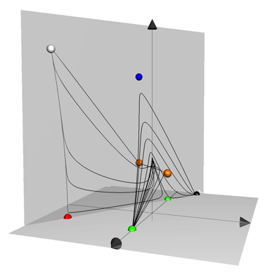
(a) $\gamma_{s_{1}}$ for $m=1$

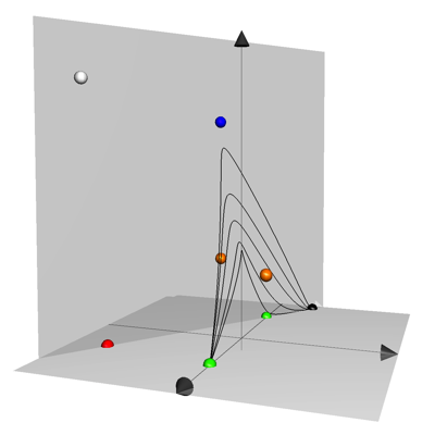
(b) $s_{1}\in\left(0,s_{\star}\right)$

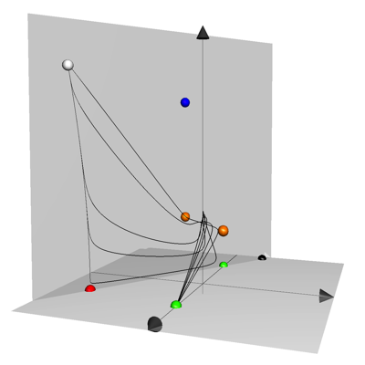
(c) $s_{2}\in\left(s_{\star},\infty\right)$

Figure 6: The set $\mathcal{S}$ is degenerate as shown in Proposition 4.2. Hence only one integral curve $\gamma_{s_{\star}}$ is known to join $p_{0}^{\pm}$ (green) and it represents the Bohm’s metric. Figures above indicate that $\gamma_{s_{1}}$ converges to $q_{1}^{-}$ (black) for $s_{1}\in(0,s_{\star})$ and converges to $q_{3}^{-}$ (white) for $s_{1}\in(s_{\star},\infty)$.

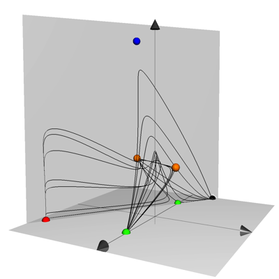
(a) $\gamma_{s_{1}}$ for $m=2$

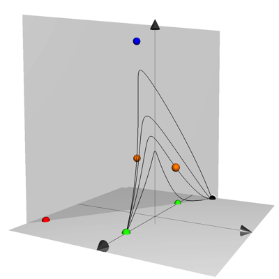
(b) $s_{1}\in\left(0,s_{\star}\right)$

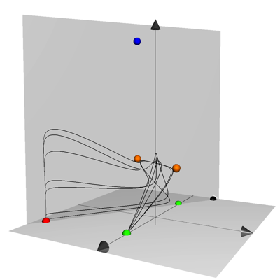
(c) $s_{2}\in\left(s_{\star},s_{\star\star}\right)$

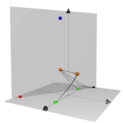
(d) $s_{2}\in(s_{\star\star},\infty)$

Figure 7: Theorem 1.1 and Theorem 1.2 claim that for $m\geq 2$ there are at least two integral curves $\gamma_{s_{\star}}$ and $\gamma_{s_{\star\star}}$ that join $p_{0}^{\pm}$ (green). Figures above indicate that $\gamma_{s_{1}}$ converges to $q_{1}^{-}$ (black) for $s_{1}\in(0,s_{\star})\cup(s_{\star\star},\infty)$ and converges to $q_{2}^{-}$ (red) for $s_{1}\in(s_{\star},s_{\star\star})$.

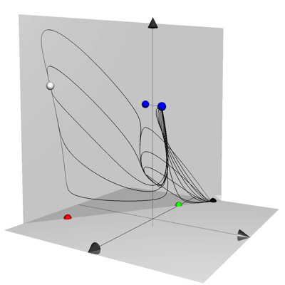
(a) $\zeta_{s_{2}}$ for $m=1$

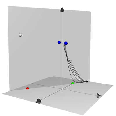
(b) $s_{2}\in\left(0,\frac{1}{2m+6}\right)$

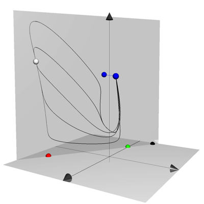
(c) $s_{2}\in\left(\frac{1}{2m+6},s_{\bullet}\right)$

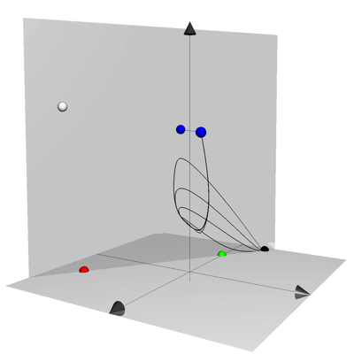
(d) $s_{2}\in(s_{\bullet},\infty)$

Figure 8: Theorem 1.3 is realized in the plots above. For $m=1$, the graph of $\zeta_{0}$ is the straight line that joins $p_{0}^{\pm}$ (blue). As $s_{2}$ increases from $0$, the integral curve $\zeta_{s_{2}}$ converges to $q_{1}^{-}$ (black), until $\zeta_{\frac{1}{2m+6}}$ converges to $p_{0}^{-}$ (green). For $s_{2}>\frac{1}{2m+6}$, the integral curve $\zeta_{s_{2}}$ converges to $q_{3}^{-}$ (white), until $s_{2}=s_{\bullet}$ once again joins $p_{0}^{\pm}$. For the $s_{2}>s_{\bullet}$, the integral curve $\zeta_{s_{2}}$ converges again to $q_{1}^{-}$.

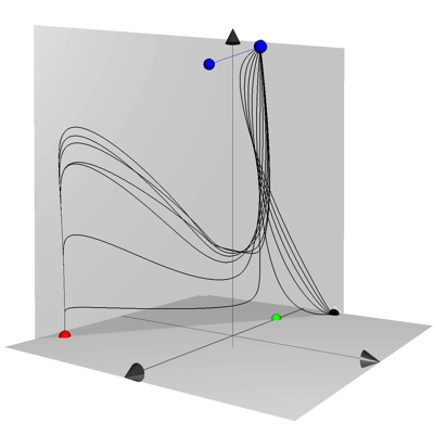
(a) $\zeta_{s_{2}}$ for $m=1$

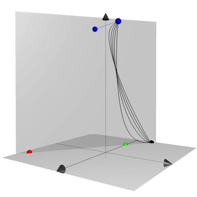
(b) $s_{2}\in\left(0,\frac{1}{2m+6}\right)$

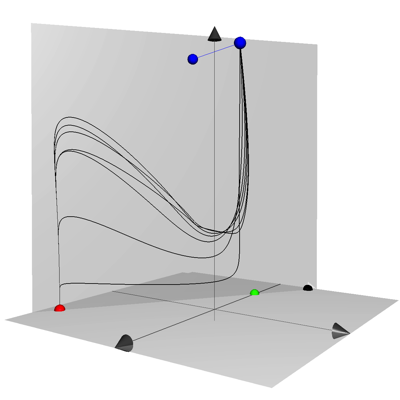
(c) $s_{2}\in\left(\frac{1}{2m+6},\infty\right)$

Figure 9: For $m\geq 2$, the behavior of $\zeta_{s_{2}}$ is relatively simpler. For $s_{2}\in\left(0,\frac{1}{2m+6}\right)$, the integral curve $\zeta_{s_{2}}$ converges to $q_{1}^{-}$ (black). For $s_{2}>\frac{1}{2m+6}$, the integral curve $\zeta_{s_{2}}$ converges to $q_{2}^{-}$ (red).

References

- [BB82] L. Bérard-Bergery. Sur de nouvelles variétés riemanniennes d’Einstein. In Institut Élie Cartan, 6, volume 6 of Inst. Élie Cartan, pages 1–60. Univ. Nancy, Nancy, 1982.
- [Böh98] C. Böhm. Inhomogeneous Einstein metrics on low-dimensional spheres and other low-dimensional spaces. Inventiones Mathematicae, 134(1):145–176, 1998.
- [BS89] R. L. Bryant and S. M. Salamon. On the construction of some complete metrics with exceptional holonomy. Duke Mathematical Journal, 58(3):829–850, 1989.
- [Chi19] H. Chi. Cohomogeneity one Einstein metrics on vector bundles. PhD Thesis, McMaster University, 2019.
- [Chi21] H. Chi. Einstein metrics of cohomogeneity one with as principal orbit. Communications in Mathematical Physics, 386:1011–1049, 2021.
- [CL55] E. A. Coddington and N. Levinson. Theory of Ordinary Differential Equations. McGraw-Hill Book Company, Inc., New York-Toronto-London, 1955.
- [DHW13] A. S. Dancer, S. J. Hall, and M. Y. Wang. Cohomogeneity one shrinking Ricci solitons: An analytic and numerical study. Asian Journal of Mathematics, 17(1):33–62, 2013.
- [EW00] J.-H. Eschenburg and M. Y. Wang. The initial value problem for cohomogeneity one Einstein metrics. The Journal of Geometric Analysis, 10(1):109–137, 2000.
- [FH17] L. Foscolo and M. Haskins. New G2-holonomy cones and exotic nearly Kähler structures on and . Annals of Mathematics, 185(1):59–130, 2017.
- [GPP90] G. W. Gibbons, D. N. Page, and C. N. Pope. Einstein metrics on and bundles. Communications in Mathematical Physics, 127(3):529–553, 1990.
- [HYI03] M. Hiragane, Y. Yasui, and H. Ishihara. Compact einstein spaces based on quaternionic k hler manifolds. Classical and Quantum Gravity, 20(18):3933–3950, 2003.
- [Jen73] G. R. Jensen. Einstein metrics on principal fibre bundles. Journal of Differential Geometry, 8(4):599–614, 1973.
- [Koi81] N. Koiso. Hypersurfaces of Einstein manifolds. Annales scientifiques de l’École normale supérieure, 14(4):433–443, 1981.
- [KS86] N. Koiso and Y. Sakane. Non-homogeneous Kähler–Einstein metrics on compact complex manifolds. In Curvature and Topology of Riemannian Manifolds, volume 1201 of Lecture Notes in Mathematics, pages 165–179, Berlin, Heidelberg, 1986. Springer.
- [KS88] N. Koiso and Y. Sakane. Non-homogeneous Kähler-Einstein metrics on compact complex manifolds. II. Osaka Journal of Mathematics, 25(4):933–959, 1988.
- [Mye41] S. B. Myers. Riemannian manifolds with positive mean curvature. Duke Mathematical Journal, 8(2):401–404, 1941.
- [Pag78] D. N. Page. A compact rotating gravitational instanton. Physics Letters B, 79(3):235–238, 1978.
- [PP86] D. N. Page and C. N. Pope. Einstein metrics on quaternionic line bundles. Classical and Quantum Gravity, 3(2):249–259, 1986.
- [PP87] D. N. Page and C. N. Pope. Inhomogeneous Einstein metrics on complex line bundles. Classical and Quantum Gravity, 4(2):213–225, 1987.
- [Sak86] Y. Sakane. Examples of compact Einstein Kähler manifolds with positive Ricci tensor. Osaka Journal of Mathematics, 23(3):585–616, 1986.
- [Win17] M. Wink. Cohomogeneity one Ricci solitons from Hopf fibrations. arXiv:1706.09712, 2017.
- [WW98] J. Wang and M.Y. Wang. Einstein metrics on -bundles. Mathematische Annalen, 310(3):497–526, 1998.
- [Zil82] W. Ziller. Homogeneous einstein metrics on spheres and projective spaces. Mathematische Annalen, 259(3):351–358, 1982.