Fractional Dynamics and Modulational Instability in Long-Range Heisenberg Chains

Abstract

We study the effective dynamics of ferromagnetic spin chains in presence of long-range interactions. We consider the Heisenberg Hamiltonian in one dimension for which the spins are coupled through power-law long-range exchange interactions with exponent $\alpha$. We add to the Hamiltonian an anisotropy in the $z$-direction. In the framework of a semiclassical approach, we use the Holstein-Primakoff transformation to derive an effective long-range discrete nonlinear Schrödinger equation. We then perform the continuum limit and we obtain a fractional nonlinear Schrödinger-like equation. Finally, we study the modulational instability of plane-waves in the continuum limit and we prove that, at variance with the short-range case, plane waves are modulationally unstable for $\alpha<3$. We also study the dependence of the modulation instability growth rate and critical wave-number on the parameters of the Hamiltonian and on the exponent $\alpha$.

Keywords: Heisenberg spin chains, long-range interactions, fractional equations, modulational instability.

I Introduction

Simplified models of magnetic systems, like the Ising model, have allowed the understanding of complex magnetic phenomena and the theoretical interpretation of phase transitions parisi1986 . Specifically, the study of low dimensional spin systems has been at the center of a constant attention in the field of magnetic materials mattis1986 ; majlis2007 ; lacroix2011 . Applications of models of magnetism cover a very wide range of phenomena, from classical and quantum transport to nuclear magnetic resonance a1 . An important role in the study of magnetic systems is played by the description of strong correlations and of the nonlinearities induced by inter-spin interactions a2 ; a3 . On the other hand, the effects of long-range interactions, where each unit is coupled to all others, motivated a remarkable activity in the last decades a16 ; campa2014 ; defenu2020 . First studies of models of classical spins with long-range interactions date back to Refs. dyson1 ; dyson2 . A typical interaction which is relevant for a number of systems, ranging from gravitational ones to dipolar magnets and gases, is provided by the power-law decay ${1}/{r^{\alpha}}$, where $r$ is the distance among constituents. It is well known that a first criterion to determine the long-range nature of a system with power-law decaying interactions is based on the comparison of $\alpha$ with the space dimension $d$. If $\alpha<d$ and if the system is homogeneous, then it displays a diverging energy density. Thus, in order to obtain a well defined thermodynamic limit, the so-called Kac rescaling of the energy is required. In the following, we will refer to this region as the non-additive or strong long-range region. If $\alpha>d$, the energy of the system is additive and it is useful to introduce a value of $\alpha$, which we denote by $\alpha^{*}$, such that for $\alpha>\alpha^{*}$ the system behaves at criticality as a short-range system sak1973 . Since $\alpha^{*}>d$, there is a region of values of $\alpha$, given by $d<\alpha<\alpha^{*}$, in which the behavior of the system significantly differs from the one of the same system with short-range interactions, although the energy is additive: such a region is the weak long-range region. The actual value of $\alpha^{*}$ depends on the specific model and the dimension $d$. As an example, for classical $O(n)$ models in $d=1$, it is known that $\alpha^{*}=2$, see e.g. thouless1969 ; a17 ; a18 . These studies have been also performed for quantum spin systems with long-range couplings dutta2001 ; defenu2017 .

A common feature for systems with long-range interactions is the behaviour of the dispersion relation as $\propto k^{\sigma}$ where $\sigma=\alpha-d$. This behaviour implies, in many cases, that the low-energy effective dynamics can be described by a fractional differential equation a15 , which involves derivatives and/or integrals of non-integer order. Such equations are used to describe anomalous kinetics, anomalous transport phenomena, etc. a19 . Fractional dynamics is a field of study which investigates the behavior of microscopic and macroscopic systems that are either characterized by power-law non locality, or by power-law long term memory. Recently, models of coupled nonlinear oscillators with long-range couplings have been introduced with the aim of understanding the role played by nonlocal interactions in several phenomena: relaxation to equilibrium Kevrekidi20 , anomalous transport Benenti21 , localized solutions Korabel20 . Among various possible examples, we can mention the Fermi-Pasta-Ulam-Tsingou model Bountis20 with long-range couplings a6 ; a7 , for which one can derive explicitly an effective fractional equation, the fractional Boussinesq equation, whose solutions depend on the long-range exponent $\alpha$.

A natural extension of these studies is to consider other models, in particular those relevant for the study of magnetism. In this paper, we investigate the Heisenberg model with long-range couplings Frohlich ; Joyce and we derive for the first time in the large-$S$ limit, $S$ being the value of the spin, a fractional nonlinear Schrödinger (FNLS) equation for the effective dynamics. To this aim, we proceed by mapping the Heisenberg spin chain with long-range interactions into a continuum equation with the Riesz fractional derivatives using the Holstein-Primakoff transformation. The final equations of motion describe the dynamics of the Heisenberg model with long-range couplings in the continuum limit. In order to show an application of the equations that we obtain, we study modulational instabilities and we discuss how the modulationally unstable and stable regions depend on the range of the power-law exponent $\alpha$. Modulational instabilities were introduced and studied in lattice models kivshar1992 ; daumont1997 ; trombettoni2001 to study the localization of energy and the stability of dynamical regimes dauxois2006 . In particular, the modulational instabilities of the discrete nonlinear Schrödinger equations with long-range couplings were considered in Ref. a20 . Here, the derivation of the effective fractional equation allows for a qualitative determination of modulationally stable regions in the space of parameters.

The paper is organized as follows. In Section II, we derive the effective Hamiltonian using bosonic operators. In Section III, we derive the FNLS equation and the corresponding integro-differential equation valid in the continuum limit. In Section IV, we study the modulational instability of plane-waves excitations. In Section V, we discuss the results and provide an outlook on future directions of investigation. In the Appendices, we present some details of the analytical computations leading to the results discussed in the main text.

II The model and the Holstein-Primakoff transformation

In order to study the dynamics of the one-dimensional (1D) Heisenberg spin chain for spins $\vec{S}=(S_{x},S_{y},S_{z})$ located on the sites of a chain, let us start by considering the Hamiltonian

$$H=-A\sum_{n=-N}^{N}{\left({S_{n}^{z}}\right)^{2}}-\sum_{-N\leq n<m\leq N}{J_{m,n}\vec{S}_{n}\cdot\vec{S}_{m}}$$ (1)

where the indices $n$ and $m$ denote the sites of the lattice and $N$ is the total number of spins. $S$ is the value of the spin. In the first term of the Hamiltonian, $A$ represents the anisotropy parameter and in the second term, the exchange interaction $J_{m,n}$ is supposed to decay algebraically with distance as a power-law

$$J_{m,n}=\frac{J}{\left|{m-n}\right|^{\alpha}}.$$ (2)

We consider a ferromagnetic chain ($J>0)$ and choose $\alpha$ in the range $1<\alpha<3$, because for smaller values, $0<\alpha\leq 1$, the Hamiltonian diverges. This latter is the non additive strong long-range region, we therefore limit in this paper to analyze the weak long-range region. For larger values, $\alpha>3$, the system in the low-energy limit is expected to display a short-range behavior, which is exactly reached only when $\alpha\to\infty$.

The cross product of the spins at two different sites can be rewritten in terms of annihilation and creation operators as follows

$$\vec{S}_{n}\,\cdot\vec{S}_{m}=\frac{1}{2}\left({S_{n}^{+}S_{m}^{-}+S_{n}^{-}S_{m}^{+}}\right)+S_{n}^{z}S_{m}^{z}.$$ (3)

We then use the Holstein-Primakoff transformation for spins operators in terms of bosonic operators in the framework of the low temperature approximation a21 ; a22 ; a23 as

$$S_{n}^{+} = \sqrt{2}\varepsilon\left({1-\frac{{\varepsilon^{2}}}{4}a_{n}^{+}a_{n}+o\left({\varepsilon^{4}}\right)}\right)a_{n}$$ (4)

$$S_{n}^{-} = \sqrt{2}\varepsilon\,a_{n}^{+}\left({1-\frac{{\varepsilon^{2}}}{4}a_{n}^{+}a_{n}+o\left({\varepsilon^{4}}\right)}\right)$$ (5)

$$S_{n}^{z} = 1-\varepsilon^{2}a_{n}^{+}a_{n},$$ (6)

where $\varepsilon=1/\sqrt{S}$. Therefore, in the limit of large $S$, substituting Eqs. (4-6) into Eq. (3), we get

$$\vec{S}_{n}\cdot\,\vec{S}_{m} = 1+\varepsilon^{2}\left(a_{n}a_{m}^{+}+a_{n}^{+}a_{m}-a_{n}^{+}a_{n}-a_{m}^{+}a_{m}\right)$$ (7)

$$-\frac{\varepsilon^{4}}{4}\left(a_{n}^{+}a_{n}a_{n}a_{m}^{+}+a_{n}a_{m}^{+}a_{m}^{+}a_{m}+a_{n}^{+}a_{n}^{+}a_{n}a_{m}+a_{n}^{+}a_{m}^{+}a_{m}a_{m}-4a_{n}^{+}a_{n}a_{m}^{+}a_{m}\right)+o\left(\varepsilon^{6}\right),$$

while

$$\left({S_{n}^{z}}\right)^{2}=1-2\varepsilon^{2}a_{n}^{+}a_{n}+\varepsilon^{4}a_{n}^{+}a_{n}a_{n}^{+}a_{n}+o\left(\varepsilon^{6}\right).$$ (8)

Hamiltonian (1) can thus be rewritten in terms of bosonic creation and annihilation operators as

$$H_{1} = -\sum_{-N\leq n<m\leq N}J_{m,n}\biggl{\{}F\left(a_{n}a_{m}^{+}+a_{n}^{+}a_{m}-a_{n}^{+}a_{n}-a_{m}^{+}a_{m}\right)-G\biggl{(}a_{n}^{+}a_{n}a_{n}a_{m}^{+}+a_{n}a_{m}^{+}a_{m}^{+}a_{m}+a_{n}^{+}a_{n}^{+}a_{n}a_{m}$$ (9)

$$\hskip 113.81102pt+a_{n}^{+}a_{m}^{+}a_{m}a_{m}-4a_{n}^{+}a_{n}a_{m}^{+}a_{m}\biggr{)}\biggr{\}}-\sum\limits_{n={\color[rgb]{0,0,0}{-N}}}^{{\color[rgb]{0,0,0}{N}}}\left(-Ta_{n}^{+}a_{n}+Ia_{n}^{+}a_{n}a_{n}^{+}a_{n}\right)+o\left(\varepsilon^{6}\right),$$

where $H_{1}=H+NA+\sum_{-N\leq n<m\leq N}J_{m,n}$ and the coupling constants are $F=\varepsilon^{2}$, $G={{F^{2}}}/{4}$, $T=2FA$, and $I=AF^{2}$. Equation (9) is a bosonic, Bose-Hubbard-like, Hamiltonian which will be used in the next Section.

III Equations of motion

The equations of motion are obtained from the Heisenberg evolution equation for a given bosonic operator $a_{n}$ as follows

$$i\hbar\dot{a}_{n}=\left[{a_{n},H}\right]\,\,,\,\,-N\leq n\leq N$$ (10)

One has to compute the different commutators arising from the previous equations to get the following nonlinear discrete equation for the bosonic operators

$$i\hbar\dot{a}_{n} = -\sum\limits_{m\neq n}{J_{mn}\left[{-F(a_{n}-a_{m})-G\left({a_{n}a_{n}a_{m}^{+}+a_{m}^{+}a_{m}a_{m}+4a_{n}^{+}a_{n}a_{m}-4a_{n}a_{m}^{+}a_{m}}\right)}\right]}$$ (11)

$$\hskip 199.16928pt+Ta_{n}-I\left({a_{n}a_{n}^{+}a_{n}+a_{n}^{+}a_{n}a_{n}}\right).$$

One can write mean-field, classical equations for the dynamics of the expectation values of the bosonic operators. One way to do it is to use the Glauber coherent states representation which are defined as $a_{n}^{+}\left|f\right\rangle=f_{n}^{*}\left|f\right\rangle$ and $a_{n}\left|f\right\rangle=f_{n}\left|f\right\rangle$ and apply it for the full equation of motion through $\left\langle f\right|i\hbar\mathop{a_{n}}\limits^{.}\left|f\right\rangle=\left\langle f\right|\left[{a_{n},H}\right]\left|f\right\rangle$. We then get the following nonlinear equations of motion for the amplitude $f_{n}$ of the spin chain excitation’s

$$i\hbar\mathop{f_{n}}\limits^{.}=\sum\limits_{m\neq n}\textsterling J_{mn}\left[{F(f_{n}-f_{m})+G\left({f_{m}^{*}f_{n}^{2}+\left|{f_{m}}\right|^{2}f_{m}+4\left|{f_{n}}\right|^{2}f_{m}-4\left|{f_{m}}\right|^{2}f_{n}}\right)}\right]+Tf_{n}-2I\left|{f_{n}}\right|^{2}f_{n}.$$ (12)

Equation (12) is a discrete cubic nonlinear Schrödinger-like equation which is the subject of our analysis in the following.

III.1 The continuum limit

Following the different steps proposed by Tarasov a13 ; Korabel20 , let us define the operation which transforms the above equation for $f_{n}(t)$ into a continuum medium equation for $f(x,t)$. We assume that $f_{n}(t)$ are Fourier coefficients of some function $\hat{f}(k,t)$. Then, we define the field $\hat{f}(k,t)$ on the interval $[-K/2,K/2]$ as

$$\hat{f}(k,t)=\sum_{n=-\infty}^{+\infty}f_{n}(t)e^{-ikx_{n}}={\cal F}_{\Delta}\{f_{n}(t)\},$$ (13)

where $x_{n}=n\Delta x$ and $\Delta x=2\pi/K$ is a distance between oscillators, and conversely

$$f_{n}(t)=\frac{1}{K}\int_{-K/2}^{+K/2}dk\ \hat{f}(k,t)e^{ikx_{n}}={\cal F}_{\Delta}^{-1}\{\hat{f}(k,t)\}.$$ (14)

These equations define a Fourier transform, which is obtained in the limit $\Delta x\rightarrow 0$ $(K\rightarrow\infty$). In order to perform this limit, let us replace the discrete set of functions $f_{n}(t)=(2\pi/K)f(x_{n},t)$ with continuous function of two variables $f(x,t)$, while letting $x_{n}=n\Delta x=2\pi n/K\rightarrow x$. Then, change the sum into an integral, and Eqs. (13) and (14) become

$$\tilde{f}(k,t) = \int_{-\infty}^{+\infty}dx\ e^{-ikx}f(x,t)={\cal F}\{f(x,t)\}$$ (15)

$$f(x,t) = \frac{1}{2\pi}\int_{-\infty}^{+\infty}dk\ e^{ikx}\tilde{f}(k,t)={\cal F}^{-1}\{\tilde{f}(k,t)\}.$$ (16)

Note that $\tilde{f}(k,t)$ is the Fourier transform of the field $f(x,t)$, and that $\hat{f}(k,t)$ is the Fourier series of $f_{n}(t)$, defined by $f_{n}(t)=(2\pi/K)f(n\Delta x,t)$.

The map of the discrete model into the continuum one can be defined by the chain of transformations $\hat{T}={\cal F}^{-1}{\cal L}\ {\cal F}_{\Delta}$, where ${\cal F}_{\Delta}$ is the Fourier series transform ${\cal F}_{\Delta}\{f_{n}(t)\}=\hat{f}(k,t)$, the passage to the limit $\Delta x\rightarrow 0$ is represented by the operator ${\cal L}\{\hat{f}(k,t)\}=\tilde{f}(k,t)$ and the inverse Fourier transform is ${\cal F}^{-1}\{\tilde{f}(k,t)\}=f(x,t)$. One has therefore

$$f_{n}(t)\xrightarrow{{\cal F}_{\Delta}}\hat{f}(k,t)\xrightarrow{{\cal L}}\tilde{f}(k,t)\xrightarrow{{\cal F}^{-1}}f(x,t)=\hat{T}\{f_{n}(t)\}.$$ (17)

After introducing the general formalism needed to perform the continuum limit, let us analyze, using these methods, the discrete description displayed in Eq. (12) and derive the corresponding continuum one. Let us begin by analytically evaluating each of the terms in this Equation. Since most of the analytic computations will be performed in the framework of the continuum limit, we will consider the limit $N\rightarrow\infty$.

To this end, let consider the first term

$$A_{1}={\sum\limits_{{\color[rgb]{0,0,0}{-N}}\leq n<m\leq{\color[rgb]{0,0,0}{N}}}{J_{m,n}.\left({f_{n}{\color[rgb]{0,0,0}(t)}-f_{m}{\color[rgb]{0,0,0}(t)}}\right)}}.$$ (18)

The computations are performed in Appendix B in the similar spirit of those in which fractional equations are derived in Refs. a12 ; a13 ; Korabel20 ; a15 ; a24 ; a25 ; a26 . We obtain

$$A_{1}=a_{\alpha}\frac{{\partial^{\alpha-1}f(x,t)}}{{\partial\left|x\right|^{\alpha-1}}}.$$ (19)

where

$$a_{\alpha}=2J\Gamma(1-\alpha)\sin\left(\pi\alpha/2\right)$$ (20)

where $\Gamma$ is the Euler gamma function and the partial Riesz derivative is defined as

$$-\frac{{\partial^{\alpha}u\left({x,t}\right)}}{{\partial\left|x\right|^{\alpha}}}=\frac{1}{{2\pi}}\int\limits_{-\infty}^{+\infty}{dp\left|p\right|^{\alpha}\hat{u}\left({p,t}\right)}e^{ipx}.$$ (21)

The following term reads

$$B = \sum\limits_{{\color[rgb]{0,0,0}{-N}}\leq n<m\leq{\color[rgb]{0,0,0}{N}}}{J_{m,n}f_{m}^{*}f_{n}^{2}}$$ (22)

$$= \left({\frac{1}{{2\pi}}}\right)^{3}\int\limits_{-\infty}^{+\infty}{\sum\limits_{{\color[rgb]{0,0,0}{-N}}\leq n<m\leq{\color[rgb]{0,0,0}{N}}}{\frac{J}{{\left|{m-n}\right|^{\alpha}}}\tilde{f}^{*}(k,t)e^{-ikm}}dk\int\limits_{-\infty}^{+\infty}{\tilde{f}(k^{{}^{\prime}},t)e^{ik^{{}^{\prime}}n}dk^{{}^{\prime}}\int\limits_{-\infty}^{+\infty}{\tilde{f}(k^{{{}^{\prime\prime}}},t)e^{ik^{{{}^{\prime\prime}}}n}dk^{{{}^{\prime\prime}}}}}}.$$ (23)

In the continuum limit $N\rightarrow{\infty}$ and setting $m-n=m^{{}^{\prime}}$, we get

$$B = \left({\frac{1}{{2\pi}}}\right)^{3}\int\limits_{-\infty}^{+\infty}{\sum\limits_{m^{{}^{\prime}}=-\infty,m^{{}^{\prime}}\neq 0}^{+\infty}{\frac{{Je^{-ikm^{{}^{\prime}}}}}{{\left|{m^{{}^{\prime}}}\right|^{\alpha}}}\tilde{f}^{*}(k,t)e^{-ikn}}dk\int\limits_{-\infty}^{+\infty}{\tilde{f}(k^{{}^{\prime}},t)e^{ik^{{}^{\prime}}n}dk^{{}^{\prime}}\int\limits_{-\infty}^{+\infty}{\tilde{f}(k^{{{}^{\prime\prime}}},t)e^{ik^{{{}^{\prime\prime}}}n}dk^{{{}^{\prime\prime}}}}}}$$ (24)

$$= \left({\frac{1}{{2\pi}}}\right)^{3}\int\limits_{-\infty}^{+\infty}{\hat{J}_{\alpha}(-k)\tilde{f}^{*}(k,t)e^{-ikn}dk\int\limits_{-\infty}^{+\infty}{\tilde{f}(k^{{}^{\prime}},t)e^{ik^{{}^{\prime}}n}dk^{{}^{\prime}}\int\limits_{-\infty}^{+\infty}{\tilde{f}(k^{{}^{\prime\prime}},t)e^{ik^{{}^{\prime\prime}}n}dk^{{}^{\prime\prime}}}}}.$$ (25)

It is useful to introduce the following function

$$\hat{J}_{\alpha}(x)=\sum\limits_{m^{{}^{\prime}}=-\infty,m^{{}^{\prime}}\neq 0}^{+\infty}J{\frac{{\displaystyle e^{im^{{}^{\prime}}x}}}{{\displaystyle\left|{m^{{}^{\prime}}}\right|^{\alpha}}}}.$$ (26)

Next, we use the so-called infrared limit approximation, which is helpful to derive the main relation that allows us to pass from the discrete medium to the continuum Korabel20 ; a12 ; a13 . For $1<\alpha<3$, $\alpha\neq 2$ and $k\longrightarrow 0$, the fractional power of $\left|{k}\right|$ is a leading asymptotic term and

$$\hat{J}_{\alpha}(-k)=\hat{J}_{\alpha}(k)\simeq a_{\alpha}\left|k\right|^{\alpha-1}+\hat{J}_{\alpha}(0).$$ (27)

This allows us to transform the nonlinear discrete equation into a fractional differential equation. In the range $1<\alpha<3$, provided $\alpha\neq 2$, we get

$$B=\left({\frac{1}{{2\pi}}}\right)^{3}a_{\alpha}\int\limits_{-\infty}^{+\infty}{\left|k\right|^{\alpha-1}\tilde{f}^{*}(k,t)e^{-ikn}dk\int\limits_{-\infty}^{+\infty}{\tilde{f}(k^{{}^{\prime}},t)e^{ik^{{}^{\prime}}n}dk^{{}^{\prime}}\int\limits_{-\infty}^{+\infty}{\tilde{f}(k^{{}^{\prime\prime}},t)e^{ik^{{}^{\prime\prime}}n}dk^{{}^{\prime\prime}}}}}+\hat{J}_{\alpha}(0)\left|{f(x,t)}\right|^{2}f(x,t).$$ (28)

Therefore, the fractional derivative allows us to write

$$B=\left({\frac{1}{{2\pi}}}\right)^{3}a_{\alpha}\int\limits_{-\infty}^{+\infty}{\left|k\right|^{\alpha-1}\tilde{f}^{*}(k,t)e^{-ikn}dk\int\limits_{-\infty}^{+\infty}{\tilde{f}(k^{{}^{\prime}},t)e^{ik^{{}^{\prime}}n}dk^{{}^{\prime}}\int\limits_{-\infty}^{+\infty}{\tilde{f}(k^{{}^{\prime\prime}},t)e^{ik^{{}^{\prime\prime}}n}dk^{{}^{\prime\prime}}}}}+\hat{J}_{\alpha}(0)\left|{f(x,t)}\right|^{2}f(x,t).$$ (29)

Thereafter, we get

$$B=-a_{\alpha}f^{2}(x,t)\frac{{\partial^{\alpha-1}f^{*}(x,t)}}{{\partial\left|x\right|^{\alpha-1}}}+\hat{J}_{\alpha}(0)\left|{f(x,t)}\right|^{2}f(x,t).$$ (30)

Following similar analytical steps, after the computations given in Appendix B, the three following terms are derived

$$C={\sum\limits_{-N\leq n<m\leq N}}{J_{mn}f_{m}\left|{f_{m}}\right|^{2}}=-a_{\alpha}\left|{f(x,t)}\right|^{2}\frac{{\partial^{\alpha-1}f(x,t)}}{{\partial\left|x\right|^{\alpha-1}}}+\hat{J}_{\alpha}(0)\left|{f(x,t)}\right|^{2}f(x,t),$$ (31)

$$D={\sum\limits_{-N\leq n<m\leq N}}{J_{mn}f_{m}\left|{f_{n}}\right|^{2}}=-a_{\alpha}\left|{f(x,t)}\right|^{2}\frac{{\partial^{\alpha-1}f(x,t)}}{{\partial\left|x\right|^{\alpha-1}}}+\hat{J}_{\alpha}(0)\left|{f(x,t)}\right|^{2}f(x,t),$$ (32)

$$E={\sum\limits_{-N\leq n<m\leq N}}{J_{mn}\left|{f_{m}}\right|^{2}f_{n}}=-a_{\alpha}\left|{f(x,t)}\right|^{2}\frac{{\partial^{\alpha-1}f(x,t)}}{{\partial\left|x\right|^{\alpha-1}}}+\hat{J}_{\alpha}(0)\left|{f(x,t)}\right|^{2}f(x,t).$$ (33)

Next, introducing the following ansatz

$$f(x,t)=\psi(x,t)\,e^{-i{{2\varepsilon^{2}At}}/{\hbar}}$$ (34)

and the parameters $U_{\alpha}=-Fa_{\alpha}$, $B_{\alpha}=Ga_{\alpha}$, $D_{\alpha}={2I-2G\hat{J}_{\alpha}(0)}$, equation (12) now reads

$$i\hbar\frac{{\partial\psi}}{{\partial t}}+U_{\alpha}\frac{{\partial^{\alpha-1}\psi}}{{\partial\left|x\right|^{\alpha-1}}}+B_{\alpha}\psi^{2}\frac{{\partial^{\alpha-1}\psi^{*}}}{{\partial\left|x\right|^{\alpha-1}}}\ +B_{\alpha}\left|\psi\right|^{2}\frac{{\partial^{\alpha-1}\psi}}{{\partial\left|x\right|^{\alpha-1}}}+D_{\alpha}\left|\psi\right|^{2}\psi=0.$$ (35)

This is a fractional cubic nonlinear Schrödinger-like equation that turns out to be the one governing the dynamics of a ferromagnetic Heisenberg spins chain involving long-range interactions in the framework of the approximation described in Appendix B, i.e. the fields $f$ are slowly varying in space.

However, if the latter approximation is avoided, then new formulas of the terms $C$ and $E$ are retrieved by the computations done in Appendix C. It follows from this analysis that we get a fractional integro-differential cubic nonlinear Schrödinger equation given by

$$i\hbar\frac{{\partial\psi}}{{\partial t}} + U_{\alpha}\frac{{\partial^{\alpha-1}\psi(x,t)}}{{\partial\left|x\right|^{\alpha-1}}}+{B_{\alpha}\psi^{2}\frac{{\partial^{\alpha-1}\psi^{*}}}{{\partial\left|x\right|^{\alpha-1}}}}+{B_{\alpha}\left|{\psi(x,t)}\right|^{2}\frac{{\partial^{\alpha-1}\psi(x,t)}}{{\partial\left|x\right|^{\alpha-1}}}}+{V_{\alpha}\left|\psi\right|^{2}\psi}$$ (36)

$$-Gb^{\alpha}\int\limits_{b}^{+\infty}dy\frac{\left|\psi(x-y,t)\right|^{2}\psi(x-y,t)+\left|\psi(x+y,t)\right|^{2}\psi(x+y,t)}{{\left|y\right|^{\alpha}}}$$

$$-4b^{\alpha}\int\limits_{b}^{+\infty}dy\frac{\left|\psi(x-y,t)\right|^{2}\psi(x,t)+\left|\psi(x+y,t)\right|^{2}\psi(x,t)}{{\left|y\right|^{\alpha}}}=0,$$

with $V_{\alpha}=-5G\hat{J}_{\alpha}(0)-2I$. Equations (35) and (36) are the main results of the present paper. The approximation done to get the differential Eq. (35) corresponds to the excitations with small amplitudes, while Eq. (36) can also describe large amplitude excitations. It would be very interesting, but nontrivial, to get their analytical solutions. This task appears not to be straightforward and in the following we focus on the modulational instability of the extended linear solutions of Eq. (35).

IV Modulational instability for the continuum medium

The modulational instability of Eq. (35) can be studied using the standard method described for example in Refs. a40 ; a41 . Here we are interested in the stability of the homogeneous solution $\psi(t)=\psi_{0}\,e^{iD_{\alpha}\psi_{0}^{2}t/\hbar}$ for which the amplitude $\psi_{0}$ is a real quantity without loss of generality. We remind that we are in the region of parameters $1<\alpha<3$, with $\alpha\neq 2$.

In the presence of a small perturbation $a(x,t)$ in the system, one can write

$$\psi(x,t)=(\psi_{0}+a)e^{iD_{\alpha}\psi_{0}^{2}t/\hbar},$$ (37)

in which $a(x,t)\ll\psi_{0}$. Substituting the ansatz (37) in Eq. (35), we obtain

$$i\hbar\frac{{\partial a}}{{\partial t}} = -U_{\alpha}\frac{{\partial^{\alpha-1}a}}{{\partial\left|x\right|^{\alpha-1}}}-{B_{\alpha}\psi_{0}(\psi_{0}+{2a})\frac{{\partial^{\alpha-1}a^{*}}}{{\partial\left|x\right|^{\alpha-1}}}}-{B_{\alpha}\psi_{0}(\psi_{0}+{a+a^{*}})\frac{{\partial^{\alpha-1}a}}{{\partial\left|x\right|^{\alpha-1}}}}-{D_{\alpha}\psi_{0}^{2}(a+a^{*})}.$$ (38)

Next, splitting the perturbation term into real and imaginary parts, $a(x,t)=u(x,t)+iv(x,t)$, and linearizing Eq. (38) with respect to $u$ and $v$, it turns out that we get the following system of equations

$$\hbar\frac{{\partial u}}{{\partial t}} = -U_{\alpha}\frac{{\partial^{\alpha-1}v}}{{\partial\left|x\right|^{\alpha-1}}},$$ (39)

$$\hbar\frac{{\partial v}}{{\partial t}} = U_{\alpha}\frac{{\partial^{\alpha-1}u}}{{\partial\left|x\right|^{\alpha-1}}}+2{B_{\alpha}\psi_{0}^{2}\frac{{\partial^{\alpha-1}u}}{{\partial\left|x\right|^{\alpha-1}}}}+2{D_{\alpha}\psi_{0}^{2}u}.$$ (40)

By introducing the following Fourier transforms

$$\hat{u}(k,t) = \int\limits_{-\infty}^{+\infty}u(x,t)\exp(ixk)dx,$$ (41)

$$\hat{v}(k,t) = \int\limits_{-\infty}^{+\infty}v(x,t)\exp(ixk)dx,$$ (42)

Equarion (39) is converted into a set of ordinary differential equations in the wavevector $k$ domain,

$$\hbar\frac{{\partial\hat{u}}}{{\partial t}} = U_{\alpha}\left|k\right|^{\alpha-1}\hat{v},$$ (43)

$$\hbar\frac{{\partial\hat{v}}}{{\partial t}} = (-U_{\alpha}-2B_{\alpha}\psi_{0}^{2})\left|k\right|^{\alpha-1}\hat{u}+2{D_{\alpha}\psi_{0}^{2}\hat{u}},$$ (44)

that can be combined into

$$\hbar\frac{{\partial^{2}\hat{v}}}{{\partial t^{2}}} = \left[2D_{\alpha}\psi_{0}^{2}-(U_{\alpha}+2B_{\alpha}\psi_{0}^{2})\left|k\right|^{\alpha-1}\right]U_{\alpha}\left|k\right|^{\alpha-1}\hat{v},$$ (45)

and the same equation for $\hat{u}$. Consequently, perturbations can grow if and only if the prefactor of the right-hand-side is positive. In such a case, one can thus define the growth rate of the modulational instability as

$$G(k,\alpha)={\sqrt{U_{\alpha}\left|k\right|^{\alpha-1}\left[2D_{\alpha}\psi_{0}^{2}-(U_{\alpha}+2B_{\alpha}\psi_{0}^{2})\left|k\right|^{\alpha-1}\right]}},$$ (46)

which shows that perturbations with wavevectors in the range of $-k_{0}<k<k_{0}$ with $k_{c}=\pm k_{0}=\pm(2D_{\alpha}\psi_{0}^{2}/(U_{\alpha}+2B_{\alpha}\psi_{0}^{2}))^{1/(\alpha-1)}$, are exponentially amplified. The growth rate, which depends on the parameters $A$ and $J$, the wavevectors $k$ and also the long-range interacting parameter $\alpha$, is definitely the quantity allowing to characterize the regions of stability/instability of the system. In this specific case, the growth rate can be zero, an imaginary number or either a positive real number. If the growth rate is zero or an imaginary number, then, the system displays stability. However if the growth rate is a real and positive number, then, the system may display a modulational instability phenomenon. Therefore, as the modulational instability phenomenon is the main focus of this study, it does occur in specific regions of the values of the parameters. Henceforth, Fig. 1 presents in green the region in the $(A,J)$ plane where the system displays the modulational instability phenomenon.

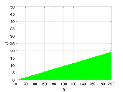
Figure 1: Here the green region corresponds the region in the $(A,J$) diagram where the modulational instability could occur.

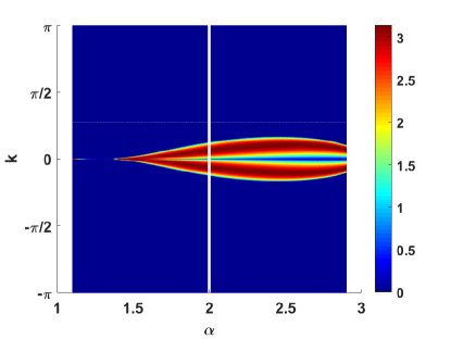
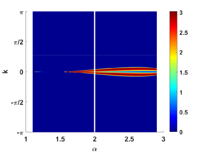
(a) (b)

Figure 2: The growth rate of the modulational instability as a function of the long-range interacting exponent $\alpha$ for different values of $J=5$ (panel a) and $J=15$ (b). Both panels are obtained for $A$=160 and $\psi_{0}=0.1$. The blue region corresponds to the stable domain while the multicolor region corresponds to the unstable one.

Figure 2 shows the dependence of the modulational instability growth rate on the wavevector $k$ and the fractional index $\alpha$ for particular values of the parameter $J$. Here, we realize that the larger is the exchange parameter $J$, the larger is the stable region.

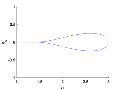
(a) (b)

Figure 3: The critical frequency $k_{c}$ as a function of the exponent $\alpha$ with $J=5$ (panel a), $J=15$ (b) and $\psi_{0}=0.1$. Both panels are obtained for $A$=160.

Our study is suitable only for non integer values of $\alpha$ between $1$ and $3$. While looking at different panels of Fig. 2 obtained for the same value of the anisotropy parameter $A$, it is realised that as the parameter $J$ increases,the range of values of $\alpha$ for which the modulational instability occurs, reduces. Figure 3 presents the evolution of the critical wave-vector as a function of the exponent $\alpha$ for the three cases presented in the previous figure. Similarly, when the parameter $J$ increases as seen in the panels of Fig. 3, the range of values of the critical wavevactor $k_{c}$ reduces.

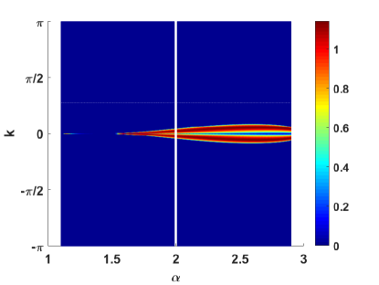
(a) (b)

Figure 4: The growth rate of the modulational instability as a function of $\alpha$ for differents values of $A=60$ (panel a) and $A=160$ (b) while the exchange parameter is fixed to $J=5$ and $\psi_{0}=0.1$. The blue region corresponds to the stable domain while the multicolor region corresponds to the unstable one.

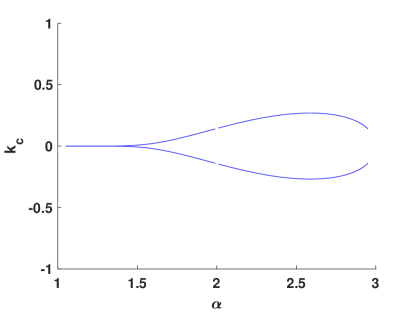
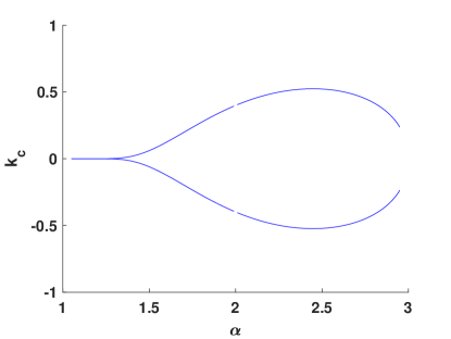
(a) (b)

Figure 5: The critical frequency $k_{c}$ as a function of the exponent $\alpha$ with $A=60$ (panel a), $A=160$ (b) and $\psi_{0}=0.1$. Both panels are obtained for $J$=5.

Figures 4 and 5 show that when the parameter $J$ is fixed and the parameter $A$ varies, the phenomenon is reversed as compared to what is observed in Fig. 2 and Fig. 3. This means, as seen in the corresponding panels, that as the anisotropy parameter increases, the instability region increases. From this, one sees that if the parameter $J$ tends to favor the stability of the system, the anisotropy parameter at variance induces the instability in such a system. Needless to mention is the fact that while looking at Fig. 2 to Fig. 5, it is realised that the power-law long-range exponent displays a minimal value below which the instability does not occur. This minimal value depends also on both the exchange parameter $J$ and the anisotropy parameter $A$. For instance, if the anisotropy parameter $A$ is fixed, the minimal value of $\alpha$ increases with increasing values of the exchange parameter $J$, as seen in panels a) and b) of Fig. 2 and Fig. 3. The dependence of the minimal value of $\alpha$ on the $A$ and $J$ is also observed when $J$ is fixed and the parameter $A$ varies as seen in panels a) and b) of Fig. 4 and Fig. 5 with a reversed effect.

V Conclusion

We have investigated the effective dynamics of a Heisenberg ferromagnetic spin chain with algebraic long-range couplings using a semiclassical approximation. We considered a spin chain with long-range power-law interactions having a strength proportional to $1/(n-m)^{\alpha}$ in the regime $1<\alpha<3$ and $\alpha\neq 2$. We have used the Holstein-Primakoff representation of the spins to derive a discrete nonlinear cubic Schrödinger equation. We have also shown how one can get, in the continuum limit, on the one hand, a fractional cubic nonlinear Schrödinger-like equation and, on the other hand, an integro-differential fractional cubic nonlinear Schrödinger-like equation, corresponding to excitations with small amplitudes and excitations with large amplitudes, respectively. This has been achieved after performing the analytical derivatives by firstly using the Riesz derivative of fractional calculus and using, secondly, a direct analysis of the Fourier spectrum in the $k\rightarrow 0$ limit. A remarkable feature of this interaction is the existence of a transformation that replaces the set of coupled individual bosonic spin equations with a continuum medium equation with a fractional spatial derivative of order $\alpha$. Such a transformation is an approximation and it appears in the infrared limit for $k\rightarrow 0$. We also studied the appearance of modulational instability using the obtained fractional equation. The modulational stability has been studied for the fractional equation and the stable and unstable regions have been determined. We showed the shifting of the onset of the modulational instability region for $\alpha>1$ and we studied the dependence of the regions of instability on the parameters of the system. It clearly appears that the modulational instability is present only for $\alpha<3$ and that above $\alpha=3$ only stable regions are present, thus indicating that the system behaves as a short range system. It is also realized that the parameter $J$ tends to favorise the stability of the system while the anisotropy parameter $A$ tends to induce the instability in the system. As a future work, it would be interesting to compare the results obtained using the effective continuum equation with those of the original lattice model. In particular it would be rewarding to compare the modulational instability regions obtained with the lattice equation found for large-$S$ with the findings presented here, since in general the lattice model is expected to have a larger region of instabilities. To what extent some unstable phases are missed by the study of the continuum fractional equation is a subject deserving future analytical and numerical studies. Finally, we observe that the approach presented here does not apply to $\alpha=2$ and it would be useful to study in detail the $\alpha\to 2$ limit.

Generalizing this one-dimensional study to 2D and 3D lattices would be very interesting and important. However, increasing the dimension of the lattice very seriously complicates the derivation of effective equations in the continuum and the search of the solutions. Problems solved in 1D have waited many years, if not decades, to be treated successfully in higher dimensions. However, this would be very helpful and important to check using numerical simulations whether modulational instability thresholds qualitatively depends on the dimension of the lattice.

Appendix A Properties of the function $J$

One thus has to compute the function

$$\hat{J}_{\alpha}(k)=\sum\limits_{m^{{}^{\prime}}=-\infty,m^{{}^{\prime}}\neq 0}^{+\infty}{\frac{{Je^{ikm^{{}^{\prime}}}}}{{\left|{m^{{}^{\prime}}}\right|^{\alpha}}}} = \sum\limits_{m^{{}^{\prime}}=-\infty}^{-1}{\frac{{Je^{ikm^{{}^{\prime}}}}}{{\left|{m^{{}^{\prime}}}\right|^{\alpha}}}}+\sum\limits_{m=1}^{+\infty}{\frac{{Je^{ikm^{{}^{\prime}}}}}{{\left|{m^{{}^{\prime}}}\right|^{\alpha}}}}$$ (47)

$$= \sum\limits_{m^{{}^{\prime}}=1}^{+\infty}{\frac{{Je^{-ikm^{{}^{\prime}}}}}{{\left|{m^{{}^{\prime}}}\right|^{\alpha}}}}+\sum\limits_{m=1}^{+\infty}{\frac{{Je^{ikm^{{}^{\prime}}}}}{{\left|{m^{{}^{\prime}}}\right|^{\alpha}}}}.$$ (48)

Introducing the poly-logarithm function defined as

$$\sum\limits_{m^{{}^{\prime}}=-\infty,m^{{}^{\prime}}\neq 0}^{+\infty}{\frac{{e^{ikm^{{}^{\prime}}}}}{{\left|{m^{{}^{\prime}}}\right|^{\alpha}}}} = {Li_{\alpha}(e^{-ik})+Li_{\alpha}\left({e^{ik}}\right)}$$ (49)

$$Li_{\alpha}\left({e^{z}}\right) = \Gamma(1-\alpha)(-z)^{\alpha-1}+\sum\limits_{n=0}^{+\infty}{\frac{{{\zeta}\left({\alpha-n}\right)}}{{n!}}z^{n}};\qquad\left|z\right|\prec 2\pi$$ (50)

in which ${\zeta}$ stands for the zeta function defined as ${\zeta}\left({\alpha}\right)=\sum\limits_{n=1}^{+\infty}{{1}/{n^{\alpha}}}$ and $z=ik\Delta x$, it turns out that we get

$$\hat{J}_{\alpha}(k) = J\left[{\Gamma(1-\alpha)\left({(-ik)^{\alpha-1}+\left({ik}\right)^{\alpha-1}}\right)+\sum\limits_{n=0}^{+\infty}{\frac{{{\zeta}\left({\alpha-n}\right)}}{{n!}}\left({\left({ik}\right)^{n}+\left({-ik}\right)^{n}}\right)}}\right]$$ (51)

$$= J\left[{\Gamma(1-\alpha)\left|k\right|^{\alpha-1}\left({(-i)^{\alpha-1}+(i)^{\alpha-1}}\right)+2\sum\limits_{n=0}^{+\infty}{\frac{{{\zeta}\left({\alpha-n}\right)}}{{(2n)!}}\left({-k^{2}}\right)^{n}}}\right]$$ (52)

$$= J\left[{\Gamma(1-\alpha)\left|k\right|^{\alpha-1}(e^{i\frac{\pi}{2}({\alpha-1})}+e^{-i\frac{\pi}{2}({\alpha-1})})+2\sum\limits_{n=0}^{+\infty}{\frac{{{\zeta}\left({\alpha-n}\right)}}{{(2n)!}}\left({-k^{2}}\right)^{n}}}\right]$$ (53)

$$= 2J\left[{\Gamma(1-\alpha)\left|k\right|^{\alpha-1}\sin(\frac{\pi}{2}\alpha)+{\zeta}\left({\alpha}\right)+\sum\limits_{n=1}^{+\infty}{\frac{{{\zeta}\left({\alpha-n}\right)}}{{(2n)!}}\left({-k^{2}}\right)^{n}}}\right].$$ (54)

Denoting $\hat{J}_{\alpha}(0)=2J{\zeta}\left({\alpha}\right)$ and $a_{\alpha}=2J\Gamma(1-\alpha)\sin\left(\pi\alpha/2\right)$, we thus get

$$\hat{J}_{\alpha}(k) = \left[{a_{\alpha}\left|k\right|^{\alpha-1}+\hat{J}_{\alpha}(0)+2J\sum\limits_{n=1}^{+\infty}{\frac{{{\zeta}\left({\alpha-n}\right)}}{{(2n)!}}\left({-k^{2}}\right)^{n}}}\right]$$ (55)

$$\hat{J}_{\alpha}(0)-\hat{J}_{\alpha}(k) = -\left[{a_{\alpha}\left|k\right|^{\alpha-1}+2J\sum\limits_{n=1}^{+\infty}{\frac{{{\zeta}\left({\alpha-n}\right)}}{{(2n)!}}\left({-k^{2}}\right)^{n}}}\right].$$ (56)

In the framework of the continuum approximation a25 , we get the expression

$$\hat{J}_{\alpha}(0)-\hat{J}_{\alpha}(k)\simeq-a_{\alpha}\left|k\right|^{\alpha-1}.$$ (57)

For non-integer $\alpha>3$ a15 , we have

$$\hat{J}_{\alpha}(k)\simeq-\left|k\right|^{2}{{\zeta}\left({\alpha-2}\right)}+\hat{J}_{\alpha}(0)$$ (58)

Appendix B Discussion of the different terms of the discrete nonlinear equation

We use the notation

$$f(x,t) =\displaystyle\frac{1}{{2\pi}}\int\limits_{-\infty}^{+\infty}\ \tilde{f}(k,t){e^{ik{\color[rgb]{0,0,0}x}}}dk\equiv\mathcal{F}^{-1}\{\tilde{f}(k,t)\}$$ (59)

$$\tilde{f}(k,t) =\displaystyle\int\limits_{-\infty}^{+\infty}\ f(x,t){e^{-ik{\color[rgb]{0,0,0}x}}}dk\equiv\mathcal{F}\{f(x,t)\},$$ (60)

where $\mathcal{F}\{f(x,t)\}$ is the Fourier transform of $f(x,t)$ with respect to $x$.

In that case, the term $A_{1}$ defined in Eq. (18) reads

$$A_{1} =\displaystyle\frac{1}{{2\pi}}\int\limits_{-\infty}^{+\infty}{\sum\limits_{m=-\infty,m\neq n}^{+\infty}{J_{m,n}}}\ \tilde{f}\left({e^{ikn}-e^{ikm}}\right)dk$$ (61)

$$\displaystyle=\frac{1}{{2\pi}}\int\limits_{-\infty}^{+\infty}{\sum\limits_{m=-\infty,m\neq n}^{+\infty}{\frac{J}{{\left|{m-n}\right|^{\alpha}}}\tilde{f}\left({k,t}\right)\left({e^{ikn}-e^{ikm}}\right)}dk}.$$ (62)

Setting then $m^{{}^{\prime}}=m-n$, we get the following expression

$$A_{1} = \frac{1}{{2\pi}}\int\limits_{-\infty}^{+\infty}{\sum\limits_{m^{{}^{\prime}}=-\infty,m^{{}^{\prime}}\neq 0}^{+\infty}{\frac{J}{{\left|{m^{{}^{\prime}}}\right|^{\alpha}}}\tilde{f}\left({k,t}\right)\left({e^{ikn}-e^{ik(m^{{}^{\prime}}+n)}}\right)}dk}$$ (63)

$$= \frac{1}{{2\pi}}\left(\int\limits_{-\infty}^{+\infty}{\sum\limits_{m^{{}^{\prime}}=-\infty,m^{{}^{\prime}}\neq 0}^{+\infty}{\frac{J}{{\left|{m^{{}^{\prime}}}\right|^{\alpha}}}\tilde{f}(k,t)e^{ikn}}dk}-\int\limits_{-\infty}^{+\infty}{\sum\limits_{m^{{}^{\prime}}=-\infty}^{+\infty}{\frac{{Je^{ikm^{{}^{\prime}}}}}{{\left|{m^{{}^{\prime}}}\right|^{\alpha}}}\tilde{f}(k,t)e^{ikn}}dk}\right)$$ (64)

$$= \frac{1}{{2\pi}}\left[{\int\limits_{-\infty}^{+\infty}{\hat{J}_{\alpha}\left(0\right)\tilde{f}(k,t)e^{ikn}dk}-\int\limits_{-\infty}^{+\infty}{\hat{J}_{\alpha}\left({k}\right)\tilde{f}(k,t)e^{ikn}}dk)}\right]$$ (65)

$$= \frac{1}{{2\pi}}\int\limits_{-\infty}^{+\infty}{(\hat{J}_{\alpha}(0)-\hat{J}_{\alpha}(k))\tilde{f}(k,t)e^{ikn}dk},$$ (66)

where we set $x=k\Delta x$ and $\hat{J}_{\alpha}(x)=\sum\limits_{m^{{}^{\prime}}=-\infty,m^{{}^{\prime}}\neq 0}^{+\infty}J{{{e^{im^{{}^{\prime}}x}}}/{{\left|{m^{{}^{\prime}}}\right|^{\alpha}}}}$. It turns out that we get

$$A_{1}=-\frac{{a_{\alpha}}}{{2\pi}}\int\limits_{-\infty}^{+\infty}{k^{\alpha-1}\hat{f}(k,t)e^{ikn}dk}.$$ (67)

Since the Fourier transform involving the absolute value of momentum $\left|k\right|^{\alpha}$ is expressed by Riesz derivative in the real space as

$$\frac{1}{{2\pi}}\int\limits_{-\infty}^{+\infty}{\left|k\right|^{\alpha}\tilde{f}(k,t)e^{ikn}dk}\simeq-\frac{{\partial^{\alpha}f(x,t)}}{{\partial\left|x\right|^{\alpha}}}$$ (68)

with $x=n\Delta x$, the term $A_{1}$ finally reads

$$A_{1}=a_{\alpha}\frac{{\partial^{\alpha-1}f(x,t)}}{{\partial\left|x\right|^{\alpha-1}}}.$$ (69)

The term $C$ can be split as

$$C=\underbrace{\sum\limits_{m=-\infty,m\neq n}^{n-1}{\frac{J}{{\left|{m-n}\right|^{\alpha}}}\left|{f_{m}}\right|^{2}f_{m}}}_{C_{1}}+\underbrace{\sum\limits_{m=n+1,m\neq n}^{+\infty}{\frac{J}{{\left|{m-n}\right|^{\alpha}}}\left|{f_{m}}\right|^{2}f_{m}}}_{C_{2}}$$ (70)

that can be analytically computed separately. Then, we get

$$C_{1}=\left({\frac{1}{{2\pi}}}\right)^{3}\int\limits_{-\infty}^{+\infty}{\sum\limits_{m=-\infty,m\neq n}^{n-1}{\frac{{Je^{ikm}}}{{\left|{m-n}\right|^{\alpha}}}}\tilde{f}(k,t)dk\int\limits_{-\infty}^{+\infty}{\tilde{f}^{*}(k^{{}^{\prime}},t)e^{-ik^{{}^{\prime}}(m)}dk^{{}^{\prime}}\int\limits_{-\infty}^{+\infty}{\tilde{f}(k^{{}^{\prime\prime}},t)e^{ik^{{}^{\prime\prime}}(m)}dk^{{}^{\prime\prime}}}}}$$ (71)

and next setting $m-n=m^{{}^{\prime}}$, it turns out that

$$C_{1} = \left({\frac{1}{{2\pi}}}\right)^{3}\int\limits_{-\infty}^{+\infty}\!\!{\sum\limits_{m^{{}^{\prime}}=-\infty,m^{{}^{\prime}}\neq 0}^{-1}\!\!\!\!\!\!{\frac{{Je^{ikm^{{}^{\prime}}}}}{{\left|{m^{{}^{\prime}}}\right|^{\alpha}}}}\tilde{f}(k,t)e^{ikn}dk\!\!\int\limits_{-\infty}^{+\infty}{\tilde{f}^{*}(k^{{}^{\prime}},t)e^{-ik^{{}^{\prime}}(m^{{}^{\prime}}+n)}dk^{{}^{\prime}}\!\!\int\limits_{-\infty}^{+\infty}{\tilde{f}(k^{{}^{\prime\prime}},t)e^{ik^{{}^{\prime\prime}}(m^{{}^{\prime}}+n)}dk^{{}^{\prime\prime}}}}}$$ (72)

$$= \left({\frac{1}{{2\pi}}}\right)^{3}\int{\int{\int_{-\infty}^{+\infty}{\sum\limits_{m^{{}^{\prime}}=1,m^{{}^{\prime}}\neq 0}^{+\infty}\!\!\!\!{\frac{{Je^{-i(k-k^{{}^{\prime}}+k^{{}^{\prime\prime}})m^{{}^{\prime}}}}}{{\left|{m^{{}^{\prime}}}\right|^{\alpha}}}}\tilde{f}(k,t)e^{ikn}\tilde{f}^{*}(k^{{}^{\prime}},t)e^{-ik^{{}^{\prime}}n}\tilde{f}(k^{{}^{\prime\prime}},t)e^{ik^{{}^{\prime\prime}}n}dkdk^{{}^{\prime}}dk^{{}^{\prime\prime}}}}}$$ (73)

$$= \left({\frac{1}{{2\pi}}}\right)^{3}\int\limits_{-\infty}^{+\infty}\!\!{\sum\limits_{m^{{}^{\prime}}=1,m^{{}^{\prime}}\neq 0}^{+\infty}\!\!\!\!\!\!{\frac{{Je^{-ikm^{{}^{\prime}}\Delta x}}}{{\left|{m^{{}^{\prime}}}\right|^{\alpha}}}}\tilde{f}(k,t)e^{ikn}dk\!\!\!\!\int\limits_{-\infty}^{+\infty}{\tilde{f}^{*}(k^{{}^{\prime}},t)e^{-ik^{{}^{\prime}}(-m^{{}^{\prime}}+n)}dk^{{}^{\prime}}\!\!\!\!\int\limits_{-\infty}^{+\infty}{\tilde{f}(k^{{}^{\prime\prime}},t)e^{ik^{{}^{\prime\prime}}(-m^{{}^{\prime}}+}dk^{{}^{\prime\prime}}}}}$$ (74)

$$C_{1} = \left({\frac{1}{{2\pi}}}\right)\int\limits_{-\infty}^{+\infty}{\sum\limits_{m^{{}^{\prime}}=1,m^{{}^{\prime}}\neq 0}^{+\infty}{\frac{{Je^{-ikm^{{}^{\prime}}}}}{{\left|{m^{{}^{\prime}}}\right|^{\alpha}}}}\tilde{f}(k,t)e^{ikn}dk}f_{n-m^{{}^{\prime}}}^{*}f_{n-m^{{}^{\prime}}}.$$ (75)

Before moving to the continuum limit, we should remind that there are terms with sums of type $\sum\limits_{m^{{}^{\prime}}}{f_{n\pm m^{{}^{\prime}}}}$. In this respect, we can proceed to the approximation based on the assumption that in these sums, the fields ${f_{n\pm m^{{}^{\prime}}}}$’s are slowly varying in space. Therefore, such terms as ${f_{n\pm m^{{}^{\prime}}}}$ can be brought outside the sums over $m^{{}^{\prime}}$ a7 . In this case, we can now write

$$C_{1}=f_{n-m^{{}^{\prime}}}^{*}f_{n-m^{{}^{\prime}}}\left({\frac{1}{{2\pi}}}\right)\int\limits_{-\infty}^{+\infty}{\sum\limits_{m^{{}^{\prime}}=1,m^{{}^{\prime}}\neq 0}^{+\infty}{\frac{{Je^{-ikm^{{}^{\prime}}}}}{{\left|{m^{{}^{\prime}}}\right|^{\alpha}}}}\tilde{f}(k,t)e^{ikn}dk}.$$ (76)

Following the same later steps, we get

$$C_{2} = \left({\frac{1}{{2\pi}}}\right)^{3}\int\limits_{-\infty}^{+\infty}{\sum\limits_{m=n+1,m^{\neq}n}^{+\infty}{\frac{{Je^{ikm}}}{{\left|{m-n}\right|^{\alpha}}}}\tilde{f}(k,t)dk\int\limits_{-\infty}^{+\infty}{\tilde{f}^{*}(k^{{}^{\prime}},t)e^{-ik^{{}^{\prime}}(m)}dk^{{}^{\prime}}\int\limits_{-\infty}^{+\infty}{\tilde{f}(k^{{}^{\prime\prime}},t)e^{ik^{{}^{\prime\prime}}(m)}dk^{{}^{\prime\prime}}}}}$$ (77)

$$= \left({\frac{1}{{2\pi}}}\right)^{3}\int\limits_{-\infty}^{+\infty}{\sum\limits_{m^{{}^{\prime}}=1,m^{{}^{\prime}}\neq 0}^{+\infty}{\frac{{Je^{ikm^{{}^{\prime}}}}}{{\left|{m^{{}^{\prime}}}\right|^{\alpha}}}}\tilde{f}(k,t)e^{ikn}dk\int\limits_{-\infty}^{+\infty}{\tilde{f}^{*}(k^{{}^{\prime}},t)e^{-ik^{{}^{\prime}}(m^{{}^{\prime}}+n)}dk^{{}^{\prime}}\int\limits_{-\infty}^{+\infty}{\tilde{f}(k^{{}^{\prime\prime}},t)e^{ik^{{}^{\prime\prime}}(m^{{}^{\prime}}+n)}dk^{{}^{\prime\prime}}}}},$$ (78)

that can be rewritten as

$$C_{2}=\left({\frac{1}{{2\pi}}}\right)\int\limits_{-\infty}^{+\infty}{\sum\limits_{m^{{}^{\prime}}=1,m^{{}^{\prime}}\neq 0}^{+\infty}{\frac{{Je^{ikm^{{}^{\prime}}}}}{{\left|{m^{{}^{\prime}}}\right|^{\alpha}}}}\tilde{f}(k,t)e^{ikn}dk}f_{n+m^{{}^{\prime}}}^{*}f_{n+m^{{}^{\prime}}}.$$ (79)

Then, if we consider here also the same approximation used above to move from Eq. (75) to Eq. (76), we get

$$C_{2}=f_{n+m^{{}^{\prime}}}^{*}f_{n+m^{{}^{\prime}}}\left({\frac{1}{{2\pi}}}\right)\int\limits_{-\infty}^{+\infty}{\sum\limits_{m^{{}^{\prime}}=1,m^{{}^{\prime}}\neq 0}^{+\infty}{\frac{{Je^{-ikm^{{}^{\prime}}}}}{{\left|{m^{{}^{\prime}}}\right|^{\alpha}}}}\tilde{f}(k,t)e^{ikn}dk}.$$ (80)

It then follows that $C$ is given by

$$C=f_{n-m^{{}^{\prime}}}^{*}f_{n-m^{{}^{\prime}}}\left({\frac{1}{{2\pi}}}\right)\int\limits_{-\infty}^{+\infty}{\sum\limits_{m^{{}^{\prime}}=1,m^{{}^{\prime}}\neq 0}^{+\infty}{\frac{{Je^{-ikm^{{}^{\prime}}}}}{{\left|{m^{{}^{\prime}}}\right|^{\alpha}}}}\tilde{f}(k,t)e^{ikn}dk}+\\ f_{n+m^{{}^{\prime}}}^{*}f_{n+m^{{}^{\prime}}}\left({\frac{1}{{2\pi}}}\right)\int\limits_{-\infty}^{+\infty}{\sum\limits_{m^{{}^{\prime}}=1,m^{{}^{\prime}}\neq 0}^{+\infty}{\frac{{Je^{ikm^{{}^{\prime}}}}}{{\left|{m^{{}^{\prime}}}\right|^{\alpha}}}}\tilde{f}(k,t)e^{ikn}dk}$$ (81)

As $n\pm m^{{}^{\prime}}\simeq n$, we get

$$C=f_{n}^{*}f_{n}\left({\frac{1}{{2\pi}}}\right)\int\limits_{-\infty}^{+\infty}{\sum\limits_{m^{{}^{\prime}}=1,m^{{}^{\prime}}\neq 0}^{+\infty}{\frac{{Je^{-ikm^{{}^{\prime}}}}}{{\left|{m^{{}^{\prime}}}\right|^{\alpha}}}}\tilde{f}(k,t)e^{ikn}dk}+f_{n}^{*}f_{n}\left({\frac{1}{{2\pi}}}\right)\int\limits_{-\infty}^{+\infty}{\sum\limits_{m^{{}^{\prime}}=1,m^{{}^{\prime}}\neq 0}^{+\infty}{\frac{{Je^{ikm^{{}^{\prime}}}}}{{\left|{m^{{}^{\prime}}}\right|^{\alpha}}}}\tilde{f}(k,t)e^{ikn}dk}$$ (82)

which leads us to

$$C = f_{n}^{*}f_{n}\left({\frac{1}{{2\pi}}}\right)\int\limits_{-\infty}^{+\infty}{\sum\limits_{m^{{}^{\prime}}=1,m^{{}^{\prime}}\neq 0}^{+\infty}{\frac{{Je^{-ikm^{{}^{\prime}}}}+{Je^{ikm^{{}^{\prime}}\Delta x}}}{{\left|{m^{{}^{\prime}}}\right|^{\alpha}}}}\tilde{f}(k,t)e^{ikn}dk}$$ (83)

$$= f_{n}^{*}f_{n}\left({\frac{1}{{2\pi}}}\right)\int\limits_{-\infty}^{+\infty}{\hat{J}_{\alpha}({k})\tilde{f}(k,t)e^{ikn}dk},$$ (84)

as

$$\hat{J}_{\alpha}\left({k}\right)={\sum\limits_{m^{{}^{\prime}}=1,m^{{}^{\prime}}\neq 0}^{+\infty}{\frac{{Je^{-ikm^{{}^{\prime}}}}+{Je^{ikm^{{}^{\prime}}}}}{{\left|{m^{{}^{\prime}}}\right|^{\alpha}}}}}.$$ (85)

Here we consider the continuum approximation done in Eq. (24) to get

$$C \simeq f_{n}^{*}f_{n}\left({\frac{1}{{2\pi}}}\right)\int\limits_{-\infty}^{+\infty}{\left(a_{\alpha}\left|k\right|^{\alpha-1}+\hat{J}_{\alpha}(0)\right)\hat{f}(k,t)e^{ikn\Delta x}dk}$$ (86)

$$= f_{n}^{*}f_{n}\left({\frac{1}{{2\pi}}}\right)\int\limits_{-\infty}^{+\infty}{a_{\alpha}\left|k\right|^{\alpha-1}}\tilde{f}(k,t)e^{ikn}dk+f_{n}^{*}f_{n}\left({\frac{1}{{2\pi}}}\right)\int\limits_{-\infty}^{+\infty}{{\hat{J}_{\alpha}(0)}\tilde{f}(k,t)e^{ikn}dk}.$$ (87)

Considering that $f_{n}=f(x=n\Delta x,t)$, the continuum approximation using the Riesz derivative gives by Eq. (21) leads us to

$$C=-a_{\alpha}\frac{{\partial^{\alpha-1}f(x,t)}}{{\partial\left|x\right|^{\alpha-1}}}\left|{f(x,t)}\right|^{2}+\hat{J}_{\alpha}(0)\left|{f(x,t)}\right|^{2}f(x,t).$$ (88)

Then splitting $E$ as follows,

$$E=\sum\limits_{m=-\infty,m\neq n}^{+\infty}{J_{mn}\left|{f_{m}}\right|^{2}f_{n}}=\underbrace{\sum\limits_{m=-\infty,m\neq n}^{n-1}{J_{mn}\left|{f_{m}}\right|^{2}f_{n}}}_{E_{1}}+\underbrace{\sum\limits_{m=n+1,m\neq n}^{+\infty}{J_{mn}\left|{f_{m}}\right|^{2}f_{n}}}_{E_{2}},$$ (89)

one has to calculate each term.

$$E_{1} = \sum\limits_{m=-\infty,m\neq n}^{n-1}{J_{mn}\left|{f_{m}}\right|^{2}f_{n}}$$ (90)

$$= \left({\frac{1}{{2\pi}}}\right)^{3}\int\limits_{-\infty}^{+\infty}{\sum\limits_{m=-\infty,m\neq n}^{n-1}{\frac{J}{{\left|{m-n}\right|^{\alpha}}}}\tilde{f}(k,t)e^{ikm}dk\int\limits_{-\infty}^{+\infty}{\tilde{f}^{*}(k^{{}^{\prime}},t)e^{-ik^{{}^{\prime}}m}dk^{{}^{\prime}}\int\limits_{-\infty}^{+\infty}{\tilde{f}(k^{{}^{\prime\prime}},t)e^{ik^{{}^{\prime\prime}}n}dk^{{}^{\prime\prime}}}}}.$$ (91)

now, setting $m-n=m^{{}^{\prime}}$, we get

$$E_{1} = \left({\frac{1}{{2\pi}}}\right)^{3}\int\limits_{-\infty}^{+\infty}{\sum\limits_{m^{{}^{\prime}}=-\infty,m^{{}^{\prime}}\neq 0}^{-1}{\frac{{Je^{ikm^{{}^{\prime}}}}}{{\left|{m^{{}^{\prime}}}\right|^{\alpha}}}}\tilde{f}(k,t)e^{ikn}dk\int\limits_{-\infty}^{+\infty}{\tilde{f}(k^{{}^{\prime}},t)e^{-ik^{{}^{\prime}}(m^{{}^{\prime}}+n)}dk^{{}^{\prime}}\int\limits_{-\infty}^{+\infty}{\tilde{f}(k^{{}^{\prime\prime}},t)e^{ik^{{}^{\prime\prime}}n}dk^{{}^{\prime\prime}}}}}$$ (92)

$$= \left({\frac{1}{{2\pi}}}\right)^{3}\int\limits_{-\infty}^{+\infty}{\sum\limits_{m^{{}^{\prime}}=-\infty,m^{{}^{\prime}}\neq 0}^{-1}{\frac{{Je^{i(k-k^{{}^{\prime}})m^{{}^{\prime}}}}}{{\left|{m^{{}^{\prime}}}\right|^{\alpha}}}}\tilde{f}(k,t)e^{ikn}dk\int\limits_{-\infty}^{+\infty}{\tilde{f}(k^{{}^{\prime}},t)e^{-ik^{{}^{\prime}}n\Delta x}dk^{{}^{\prime}}\int\limits_{-\infty}^{+\infty}{\tilde{f}(k^{{}^{\prime\prime}},t)e^{ik^{{}^{\prime\prime}}n}dk^{{}^{\prime\prime}}}}}$$ (93)

$$= \left({\frac{1}{{2\pi}}}\right)^{3}\int\limits_{-\infty}^{+\infty}{\sum\limits_{m^{{}^{\prime}}=1,m^{{}^{\prime}}\neq 0}^{+\infty}{\frac{{Je^{-i(k-k^{{}^{\prime}})m^{{}^{\prime}}}}}{{\left|{m^{{}^{\prime}}}\right|^{\alpha}}}}\tilde{f}(k,t)e^{ikn}dk\int\limits_{-\infty}^{+\infty}{\tilde{f}(k^{{}^{\prime}},t)e^{-ik^{{}^{\prime}}n\Delta x}dk^{{}^{\prime}}\int\limits_{-\infty}^{+\infty}{\tilde{f}(k^{{}^{\prime\prime}},t)e^{ik^{{}^{\prime\prime}}n}dk^{{}^{\prime\prime}}}}}$$ (94)

$$= \left({\frac{1}{{2\pi}}}\right)^{3}\int\limits_{-\infty}^{+\infty}{\sum\limits_{m^{{}^{\prime}}=1,m^{{}^{\prime}}\neq 0}^{+\infty}{\frac{{Je^{-ikm^{{}^{\prime}}}}}{{\left|{m^{{}^{\prime}}}\right|^{\alpha}}}}\tilde{f}(k,t)e^{ikn}dk\int\limits_{-\infty}^{+\infty}{\tilde{f}(k^{{}^{\prime}},t)e^{-ik^{{}^{\prime}}(n-m^{{}^{\prime}})}dk^{{}^{\prime}}\int\limits_{-\infty}^{+\infty}{\tilde{f}(k^{{}^{\prime\prime}},t)e^{ik^{{}^{\prime\prime}}n}dk^{{}^{\prime\prime}}}}}$$ (95)

$$= \left({\frac{1}{{2\pi}}}\right)\int\limits_{-\infty}^{+\infty}{\sum\limits_{m^{{}^{\prime}}=1,m^{{}^{\prime}}\neq 0}^{+\infty}{\frac{{Je^{-ikm^{{}^{\prime}}}}}{{\left|{m^{{}^{\prime}}}\right|^{\alpha}}}}\tilde{f}(k,t)e^{ikn}dk}f_{n-m^{{}^{\prime}}}^{*}f_{n}.$$ (96)

Then, proceeding to the same approximation used to move from Eq. (75) to Eq. (76), we get

$$E_{1}=\left({\frac{1}{{2\pi}}}\right)f_{n-m^{{}^{\prime}}}^{*}f_{n}\int\limits_{-\infty}^{+\infty}{\sum\limits_{m^{{}^{\prime}}=1,m^{{}^{\prime}}\neq 0}^{+\infty}{\frac{{Je^{-ikm^{{}^{\prime}}}}}{{\left|{m^{{}^{\prime}}}\right|^{\alpha}}}}\tilde{f}(k,t)e^{ikn}dk}.$$ (97)

Through the same approximation and very similar steps, one derives

$$E_{2}=\left({\frac{1}{{2\pi}}}\right)f_{n+m^{{}^{\prime}}}^{*}f_{n}\int\limits_{-\infty}^{+\infty}{\sum\limits_{m^{{}^{\prime}}=1,m^{{}^{\prime}}\neq 0}^{+\infty}{\frac{{Je^{ikm^{{}^{\prime}}}}}{{\left|{m^{{}^{\prime}}}\right|^{\alpha}}}}\tilde{f}(k,t)e^{ikn}dk}$$ (98)

that leads to

$$E = \left({\frac{1}{{2\pi}}}\right)f_{n-m^{{}^{\prime}}}^{*}f_{n}\int\limits_{-\infty}^{+\infty}{\sum\limits_{m^{{}^{\prime}}=1,m^{{}^{\prime}}\neq 0}^{+\infty}{\frac{{Je^{-ikm^{{}^{\prime}}}}}{{\left|{m^{{}^{\prime}}}\right|^{\alpha}}}}\tilde{f}(k,t)e^{ikn\Delta x}dk}$$ (99)

$$+\left({\frac{1}{{2\pi}}}\right)f_{n+m^{{}^{\prime}}}^{*}f_{n}\int\limits_{-\infty}^{+\infty}{\sum\limits_{m^{{}^{\prime}}=1,m^{{}^{\prime}}\neq 0}^{+\infty}{\frac{{Je^{ikm^{{}^{\prime}}}}}{{\left|{m^{{}^{\prime}}}\right|^{\alpha}}}}\tilde{f}(k,t)e^{ikn}dk}$$

$$= \left({\frac{1}{{2\pi}}}\right)f_{n}^{*}f_{n}\int\limits_{-\infty}^{+\infty}{\sum\limits_{m^{{}^{\prime}}=1,m^{{}^{\prime}}\neq 0}^{+\infty}{\frac{{Je^{-ikm^{{}^{\prime}}}}+{Je^{ikm^{{}^{\prime}}\Delta x}}}{{\left|{m^{{}^{\prime}}}\right|^{\alpha}}}}\tilde{f}(k,t)e^{ikn}dk}$$ (100)

$$= \left({\frac{1}{{2\pi}}}\right)f_{n}^{*}f_{n}\int\limits_{-\infty}^{+\infty}{\hat{J}_{\alpha}({k})\tilde{f}(k,t)e^{ikn\Delta x}dk}$$ (101)

$$= f_{n}^{*}f_{n}\left({\frac{1}{{2\pi}}}\right)\int\limits_{-\infty}^{+\infty}{a_{\alpha}(k)^{\alpha-1}}\tilde{f}(k,t)e^{ikn}dk+f_{n}^{*}f_{n}\left({\frac{1}{{2\pi}}}\right)\int\limits_{-\infty}^{+\infty}{{\hat{J}_{\alpha}(0)}\tilde{f}(k,t)e^{ikn}dk}.$$ (102)

When we replace all these terms in the equation of motion (12), we get

$$i\hbar\dot{f} = Fa_{\alpha}\frac{{\partial^{\alpha-1}f(x,t)}}{{\partial\left|x\right|^{\alpha-1}}}-Tf+2I\left|f\right|^{2}f$$ (103)

$$+G\left[{-a_{\alpha}\frac{{\partial^{\alpha-1}f^{*}}}{{\partial\left|x\right|^{\alpha-1}}}\ +\hat{J}_{\alpha}(0)\left|f\right|^{2}f-a_{\alpha}\left|f\right|^{2}\frac{{\partial^{\alpha-1}f}}{{\partial\left|x\right|^{\alpha-1}}}+\hat{J}_{\alpha}(0)\left|f\right|^{2}f+4\hat{J}_{\alpha}(0)\left|f\right|^{2}f-4\hat{J}_{\alpha}(0)\left|f\right|^{2}f}\right].$$

Appendix C The fractional integro-differential nonlinear equation

One has

$$C = \left({\frac{1}{{2\pi}}}\right)\int\limits_{-\infty}^{+\infty}{\sum\limits_{m^{{}^{\prime}}=1,m^{{}^{\prime}}\neq 0}^{+\infty}{\frac{{Je^{-ikm^{{}^{\prime}}}}}{{\left|{m^{{}^{\prime}}}\right|^{\alpha}}}}\tilde{f}(k,t)e^{ikn}dk}f_{n-m^{{}^{\prime}}}^{*}f_{n-m^{{}^{\prime}}}+\left({\frac{1}{{2\pi}}}\right)\int\limits_{-\infty}^{+\infty}{\sum\limits_{m^{{}^{\prime}}=1,m^{{}^{\prime}}\neq 0}^{+\infty}{\frac{{Je^{ikm^{{}^{\prime}}}}}{{\left|{m^{{}^{\prime}}}\right|^{\alpha}}}}\tilde{f}(k,t)e^{ikn}dk}f_{n+m^{{}^{\prime}}}^{*}f_{n+m^{{}^{\prime}}}$$ (104)

$$= \left({\frac{1}{{2\pi}}}\right)\sum\limits_{m^{{}^{\prime}}=1,m^{{}^{\prime}}\neq 0}^{+\infty}f_{n-m^{{}^{\prime}}}^{*}f_{n-m^{{}^{\prime}}}\int\limits_{-\infty}^{+\infty}{{\frac{{Je^{ik(n-m^{{}^{\prime}})}}}{{\left|{m^{{}^{\prime}}}\right|^{\alpha}}}}\tilde{f}(k,t)dk}+\left({\frac{1}{{2\pi}}}\right)\sum\limits_{m^{{}^{\prime}}=1,m^{{}^{\prime}}\neq 0}^{+\infty}f_{n+m^{{}^{\prime}}}^{*}f_{n+m^{{}^{\prime}}}\int\limits_{-\infty}^{+\infty}{{\frac{{Je^{ik(m^{{}^{\prime}}+n)}}}{{\left|{m^{{}^{\prime}}}\right|^{\alpha}}}}\tilde{f}(k,t)dk}.$$

In the continuum limit $\Delta x\rightarrow 0$, by replacing $n$ and $m$ respectively by ${x}/{\Delta x}$ and ${y}/{\Delta x}$, we get

$$C = \left({\frac{1}{{2\pi}}}\right)\int\limits_{b}^{+\infty}dy\left|f(x-y,t)\right|^{2}\int\limits_{-\infty}^{+\infty}{{\frac{{Je^{i\frac{k}{b}(x-y)}}}{{\left|{\frac{y}{b}}\right|^{\alpha}}}}\tilde{f}(k,t)dk}+\left({\frac{1}{{2\pi}}}\right)\int\limits_{b}^{+\infty}dy\left|f(x+y,t)\right|^{2}\int\limits_{-\infty}^{+\infty}{{\frac{{Je^{i\frac{k}{b}(x+y)}}}{{\left|{\frac{y}{b}}\right|^{\alpha}}}}\tilde{f}(k,t)dk}$$ (105)

$$= \left({\frac{1}{{2\pi}}}\right)\int\limits_{b}^{+\infty}dy\left|f(x-y,t)\right|^{2}b^{\alpha}\int\limits_{-\infty}^{+\infty}{{\frac{{Je^{ip(x-y)}}}{{\left|y\right|^{\alpha}}}}\tilde{f}(k,t)dk}+\left({\frac{1}{{2\pi}}}\right)\int\limits_{b}^{+\infty}dy\left|f(x+y,t)\right|^{2}b^{\alpha}\int\limits_{-\infty}^{+\infty}{{\frac{{Je^{ip(x+y)}}}{{\left|y\right|^{\alpha}}}}\tilde{f}(k,t)dk}$$

$$= b^{\alpha}\int\limits_{b}^{+\infty}dy\frac{\left|f(x-y,t)\right|^{2}f(x-y,t)+\left|f(x+y,t)\right|^{2}f(x+y,t)}{{\left|y\right|^{\alpha}}}.$$

where $b=\Delta x$ and $p={k}/{b}$. In the same spirit of analytical computations, the term $E$ will be given by

$$E = \left({\frac{1}{{2\pi}}}\right)\sum\limits_{m^{{}^{\prime}}=1,m^{{}^{\prime}}\neq 0}^{+\infty}f_{n-m^{{}^{\prime}}}^{*}f_{n}\int\limits_{-\infty}^{+\infty}{{\frac{{Je^{ik(n-m^{{}^{\prime}})}}}{{\left|{m^{{}^{\prime}}}\right|^{\alpha}}}}\tilde{f}(k,t)dk}+\left({\frac{1}{{2\pi}}}\right)\sum\limits_{m^{{}^{\prime}}=1,m^{{}^{\prime}}\neq 0}^{+\infty}f_{n+m^{{}^{\prime}}}^{*}f_{n}\int\limits_{-\infty}^{+\infty}{{\frac{{Je^{ik(m^{{}^{\prime}}+n)}}}{{\left|{m^{{}^{\prime}}}\right|^{\alpha}}}}\tilde{f}(k,t)dk}$$ (106)

$$= b^{\alpha}\int\limits_{b}^{+\infty}dy\frac{\left|f(x-y,t)\right|^{2}f(x,t)+\left|f(x+y,t)\right|^{2}f(x,t)}{{\left|y\right|^{\alpha}}}.$$

We get the following fractional integro-differential cubic nonlinear equation given by

$$i\hbar\dot{f} = Fa_{\alpha}\frac{{\partial^{\alpha-1}f(x,t)}}{{\partial\left|x\right|^{\alpha-1}}}-Ga_{\alpha}f^{2}\frac{{\partial^{\alpha-1}f^{*}}}{{\partial\left|x\right|^{\alpha-1}}}-Ga_{\alpha}\left|{f(x,t)}\right|^{2}\frac{{\partial^{\alpha-1}f(x,t)}}{{\partial\left|x\right|^{\alpha-1}}}+5\hat{J}_{\alpha}(0)f\left|f\right|^{2}-Tf+2I\left|f\right|^{2}f$$

$$+G\left[{b^{\alpha}\int\limits_{b}^{+\infty}dy\frac{\left|f(x-y,t)\right|^{2}f(x-y,t)+\left|f(x+y,t)\right|^{2}f(x+y,t)}{{\left|y\right|^{\alpha}}}}\right]$$

$$+G\left[{4b^{\alpha}\int\limits_{b}^{+\infty}dy\frac{\left|f(x-y,t)\right|^{2}f(x,t)+\left|f(x+y,t)\right|^{2}f(x,t)}{{\left|y\right|^{\alpha}}}}\right].$$

Next, while introducing the following Ansatz:

$$f(x,t)=\psi(x,t)\,e^{-i{{2\varepsilon^{2}At}}/{\hbar}}$$ (108)

We get the integro-fractional differential nonlinear Schrödinger equation given by Eq. (36).