Nonparametric drift estimation from diffusions with correlated brownian motions

Abstract

In the present paper, we consider that $N$ diffusion processes $X^{1},\dots,X^{N}$ are observed on $[0,T]$, where $T$ is fixed and $N$ grows to infinity. Contrary to most of the recent works, we no longer assume that the processes are independent. The dependency is modeled through correlations between the Brownian motions driving the diffusion processes. A nonparametric estimator of the drift function, which does not use the knowledge of the correlation matrix, is proposed and studied. Its integrated mean squared risk is bounded and an adaptive procedure is proposed. Few theoretical tools to handle this kind of dependency are available, and this makes our results new. Numerical experiments show that the procedure works in practice.

1 Introduction

We start by describing our model. Consider the diffusion process $X=(X_{t})_{t\in[0,T]}$, defined by

$$X_{t}=x_{0}+\int_{0}^{t}b(X_{s})ds+\int_{0}^{t}\sigma(X_{s})dB_{s}\textrm{ $;$ }t\in[0,T],$$ (1)

where $x_{0}\in\mathbb{R}$, $B=(B_{t})_{t\in[0,T]}$ is a Brownian motion, $b:\mathbb{R}\rightarrow\mathbb{R}$ is a Lipschitz continuous function, and $\sigma:\mathbb{R}\rightarrow\mathbb{R}$ is a bounded Lipschitz continuous function. Now, let $B^{1},\dots,B^{N}$ be $N\in\mathbb{N}/\{0\}$ copies of $B$ such that

$$\mathbb{E}(B_{s}^{i}B_{t}^{k})=R_{i,k}(s\wedge t)\textrm{ $;$ }\forall i,k\in\{1,\dots,N\}\textrm{, }\forall s,t\in[0,T],$$ (2)

where $R=(R_{i,k})_{i,k}$ is a correlation matrix. Note that, thanks to the (stochastic) integration by parts formula, the dependence condition (2) on $B^{1},\dots,B^{N}$ implies that, for every $i,k\in\{1,\dots,N\}$, $d\langle B^{i},B^{k}\rangle_{t}=R_{i,k}dt$, with $R_{i,i}=1$. Finally, consider $X^{i}:=\mathcal{I}(x_{0},B^{i})$ for every $i\in\{1,\dots,N\}$, where $\mathcal{I}(.)$ is the Itô map associated to Equation (1). In the present paper, we consider that these $N$ diffusion processes $X^{1},\dots,X^{N}$ are observed on $[0,T]$, where $T$ is fixed and $N$ grows to infinity, and our aim is to estimate nonparametrically the drift function $b(.)$.

In the case of independent Brownian motions, that is $R=\mathbf{I}_{N}$ (the $N\times N$ identity matrix), projection least squares estimator have been studied in Comte and Genon-Catalot [7] for continuous time observations, in Denis el al. [14] for discrete time (with small step) observations with a classification purpose in the parametric setting, and in Denis et al. [15] in the nonparametric context, for instance. Marie and Rosier [20] propose a kernel based Nadaraya-Watson estimator of the drift function $b$, with bandwidth selection relying on the Penalization Comparison to Overfitting (PCO) criterion recently introduced by Lacour et al. [18]. Still in the case $R=\mathbf{I}_{N}$, Comte and Marie [12] investigate the properties of the projection least squares estimator of the drift when $B$ is a fractional Brownian motion.
Dependency is often encountered in recent works in the context of stochastic systems of $N$ interacting particles, with recent nonparametric drift estimators proposals in Della Maestra and Hoffmann [13], Belomestny et al. [3] or Comte and Genon-Catalot [9]. These kinds of models are related to physics. We rather have in mind economic or financial models. For instance, in Duellmann et al. [16], the authors consider a portfolio of $N$ homogenous firms such that the asset value $X_{t}^{i}$ at time $t$ of the $i$-th firm is modeled by Merton’s model (see [21]) $dX_{t}^{i}=\mu X_{t}^{i}dt+\sigma X_{t}^{i}dB_{t}^{i}$ with $X_{0}^{i}=X_{0}$, which corresponds to (1) with $b(x)=\mu x$ and $\sigma(x)=\sigma x$. Intending to capture the dependency between the firms, they also assume that $dB_{t}^{i}=\sqrt{\rho}dW_{t}+\sqrt{1-\rho}dW_{t}^{i}$, where $W$ is a common systematic risk factor, $W^{i}$ is a firm-specific risk factor and $\rho\in[0,1]$. This corresponds to a particular matrix $R$, precisely $R_{i,k}=\rho$ for $i\neq k$ (and $R_{i,i}=1$), so that one single parameter $\rho$ represents the so-called asset correlation. This model has been considered in e.g. Bush et al. [4], for the more mathematical purpose of studying the limit of the empirical distribution of the $X_{t}^{i}$’s (see also references therein). Our extension from specific geometric Brownian motion to general nonparametric diffusion (1), and from one single correlation parameter to a general matrix representation, is therefore standard in both respects. This context has nevertheless never been considered before up to our knowledge. Let us emphasize that our aim is not to estimate $R$, but to exhibit conditions on it such that $b(.)$ can be estimated with performance near of the independent setting.

In our framework, $T$ is fixed, and $N$ is large. Our results are nonasymptotic, but the idea is that $N$ grows to infinity. We fix a subset $I$ of $\mathbb{R}$ and build a collection of projection least squares estimators of $b_{I}=b\mathbf{1}_{I}$ where $I$ is compact or not. The estimators are defined by their coefficients on an orthonormal basis of $\mathbb{L}^{2}(I)$, $\varphi_{1},\dots,\varphi_{m}$, resulting from a standard least squares computation. Precisely, we consider the estimator of the drift function $b$ minimizing the objective function $\gamma_{N}(\tau)$

$$\tau\longmapsto\gamma_{N}(\tau):=\frac{1}{NT}\sum_{i=1}^{N}\left(\int_{0}^{T}\tau(X_{s}^{i})^{2}ds-2\int_{0}^{T}\tau(X_{s}^{i})dX_{s}^{i}\right)$$ (3)

on the $m$-dimensional function space $\mathcal{S}_{m}={\rm span}\{\varphi_{1},\dots,\varphi_{m}\}$. The first part of $\gamma_{N}(\tau)$ involves a quantity

$$\|\tau\|_{N}^{2}:=\frac{1}{NT}\sum_{i=1}^{N}\int_{0}^{T}\tau(X_{s}^{i})^{2}ds,$$

which is considered as the squared empirical norm of the function $\tau$. These estimators are the same as in Comte and Genon-Catalot [7], but their study is made significantly more difficult by the dependency context. We do not have at our disposal any coupling method nor any transformation leading to a simpler system; in particular, applying $R^{-1/2}$ to the system does not bring any simplification because of a ”widespreading” of the components of the process. Tropp’s deviation inequalities used in the independent context (see Tropp [24], Matrix Chernov Inequality, Theorem 1.1 and Matrix Bernstein Inequality, Theorem 1.4), which allow to consider the empirical norm and its expectation (an integral norm, thus) as equivalent with high probability, no longer apply. Martingale properties still are useful, and we turn to Azuma’s matrix deviation inequality (see Tropp [24], Theorem 7.1), which however requires to set sparsity conditions on $R$ (see Assumption 3). This equivalence property between empirical and weighted integral norms is the key of the rigorous study of the risk of the drift estimator, and the correlation matrix is therefore at the heart of the proofs.

The plan of the paper is the following. A first parametric example motivates the model and the way of estimating a drift parameter in Section 2. The general nonparametric drift estimator is defined in Section 3 and a risk bound on a fixed projection space is proved. Adaptive estimation is studied in Section 4 and the whole procedure is illustrated through simulations in Section 5. Lastly, proofs are gathered in Section 6.

2 Preliminary motivation and example in the parametric framework

This preliminary section deals with the geometric model described in the introduction, in the parametric framework, in order to motivate our investigations. Similarly to Duellmann et al. [16], consider $N$ risky assets of same nature and of prices processes $X^{1},\dots,X^{N}$ observed on the time interval $[0,T]$. Since these assets are of same nature, to model their prices by $dX_{t}^{i}=\mu X_{t}^{i}dt+\sigma X_{t}^{i}dB_{t}^{i}$ with $\mu\in\mathbb{R}$ and $\sigma>0$ not depending on $i\in\{1,\dots,N\}$ is realistic, but it is also very realistic to consider that $B^{1},\dots,B^{N}$ may be dependent, through the correlation matrix described above. Let us compute the quadratic risk of the least squares estimator $\widehat{\theta}_{N}$ of $\theta=\mu-\sigma^{2}/2$ in this special case. Since we can write that $X_{t}^{i}=x_{0}\exp(Y_{t}^{i})$ with $Y_{t}^{i}=\theta t+\sigma B_{t}^{i}$ for every $i\in\{1,\dots,N\}$ and $t\in[0,T]$, we set

$$\widehat{\theta}_{N}=\frac{1}{NT}\sum_{i=1}^{N}Y_{T}^{i}=\theta+\frac{\sigma}{NT}\sum_{i=1}^{N}B_{T}^{i}.$$

Then,

$$\mathbb{E}(|\widehat{\theta}_{N}-\theta|^{2}) = \frac{\sigma^{2}}{N^{2}T^{2}}\left[\sum_{i=1}^{N}\mathbb{E}(|B_{T}^{i}|^{2})+\sum_{i\neq k}\mathbb{E}(B_{T}^{i}B_{T}^{k})\right]$$

$$= \frac{\sigma^{2}}{NT}+\frac{\sigma^{2}}{N^{2}T}\sum_{i\neq k}R_{i,k}=\frac{\sigma^{2}}{NT}\left(1+\frac{1}{N}\sum_{i\neq k}R_{i,k}\right).$$

This means that the rate of convergence of $\widehat{\theta}_{N}$ is of order

$$\mathbf{V}:=\frac{1}{N}+\frac{1}{N^{2}}\sum_{i\neq k}R_{i,k}.$$

We note that if $R_{i,k}=\rho$ for all $i\neq k$, then the estimator is not consistent. This would be the same if all the coefficients of $R$ were positive and only bounded by a constant $\rho>0$. However, if we set a sparsity condition by saying that $R$ is block-diagonal with blocks of size (less than) $k_{0}$, and if we assume that all nonzero coefficients are equal to (or bounded by) $\rho$, then $\sum_{i\neq k}R_{i,k}\leqslant k_{0}\rho N$. So, $k_{0}\rho$ is the loss in risk due to dependency, while the rate remains $O(1/N)$. Referring to the firms model of Duellmann et al. [16] and Bush et al.[4], this means for instance that for a large $N$, dependent firms have to be grouped as several independent sets aggregated in the global model.

Another way to model the dependency with few parameters is to assume that

$$dB_{t}^{i}=\sqrt{\tt a}dW_{t}^{i}+\sqrt{1-\texttt{a}}dW_{t}^{i+1},$$

where $W^{1},\dots,W^{N+1}$ are independent Brownian motions and $\texttt{a}\in[0,1]$. This is a way of saying that each firm is correlated to the following one in the list. In that case,

$$R_{i,i+1}=R_{i,i-1}=\sqrt{{\tt a}(1-{\tt a})},\quad R_{i,i}=1,\quad R_{i,k}=0\textrm{ for }|k-i|>1;$$

and then

$${\bf V}=\frac{1}{N}\left(1+2\left(1-\frac{1}{N}\right)\sqrt{{\tt a}(1-{\tt a})}\right)$$

has order $O(1/N)$. Note that this matrix is sparse in the sense of Assumption 3 below.

Our purpose is to show that, at least for some special dependence schemes on $B^{1},\dots,B^{N}$, the variance term of the projection (nonparametric) least squares estimator of $b(.)$ introduced in the following section is at most of order

$$\frac{1}{N}\left(1+\frac{1}{N}\sum_{i\neq k}|R_{i,k}|\right).$$

It is noteworthy that the estimator $\widehat{\theta}_{N}$ is the maximum likelihood estimator (MLE) when $X^{1},\dots,X^{N}$ are independent, while the MLE in our dependent setting would involve – and thus require the complete knowledge of – the matrix $R$ (more specifically, its inverse). In the present strategy, the knowledge of $R$ is not required, which is interesting and may justify a loss of efficiency.

3 A projection least squares estimator of the drift function

3.1 The objective function

Set $N_{T}:=[NT]+1$ and let $f_{T}$ be the density function defined by

$$f_{T}(x):=\frac{1}{T}\int_{0}^{T}p_{s}(x_{0},x)ds\textrm{ $;$ }\forall x\in\mathbb{R},$$

where $p_{s}(x_{0},.)$ is the density with respect to Lebesgue’s measure of the probability distribution of $X_{s}$ for every $s\in(0,T]$. Let us consider the projection space $\mathcal{S}_{m}:={\rm span}\{\varphi_{1},\dots,\varphi_{m}\}$, where $\varphi_{1},\dots,\varphi_{N_{T}}$ are continuous functions from $I$ into $\mathbb{R}$ such that $(\varphi_{1},\dots,\varphi_{N_{T}})$ is an orthonormal family in $\mathbb{L}^{2}(I,dx)$, and $I\subset\mathbb{R}$ is a non-empty interval. We recall now that the objective function $\tau\in\mathcal{S}_{m}\mapsto\gamma_{N}(\tau)$ is defined by (3), where $m\in\{1,\dots,N_{T}\}$. We choose a contrast which is the same as in the independent case. Note that for the nonparametric estimation of the drift function from $N$ observed paths, even in the independent case, least squares and maximum likelihood strategies do not match. Indeed, the likelihood would involve weights $\sigma(X_{s}^{i})^{-2}$ inside all integrals. In the dependent case, there would also be the matrix $R^{-1}$ to take into account. Even if both $\sigma(.)$ and $R$ can be considered as known, it is interesting not to need them to compute the drift estimator. In particular, the step to discrete time high frequency data is then much simpler. Since the strategy works in the independent case, we can hope that if the correlations are not too strong, then the strategy remains relevant.

Remark. For any $\tau\in\mathcal{S}_{m}$,

$$\mathbb{E}(\gamma_{N}(\tau)) = \frac{1}{T}\int_{0}^{T}\mathbb{E}(|\tau(X_{s})-b(X_{s})|^{2})ds-\frac{1}{T}\int_{0}^{T}\mathbb{E}(b(X_{s})^{2})ds$$

$$= \int_{-\infty}^{\infty}(\tau(x)-b(x))^{2}f_{T}(x)dx-\int_{-\infty}^{\infty}b(x)^{2}f_{T}(x)dx.$$

Then, the more $\tau$ is close to $b$, the smaller $\mathbb{E}(\gamma_{N}(\tau))$. For this reason, the estimator of $b$ minimizing $\gamma_{N}(.)$ is studied in this paper.

3.2 The projection least squares estimator and some related matrices

In this section, $m$ is a fixed integer in $\{1,\dots,N_{T}\}$. We consider the estimator

$$\widehat{b}_{m}:=\arg\min_{\tau\in\mathcal{S}_{m}}\gamma_{N}(\tau)$$ (4)

of $b$, if it exists and is unique. Since $\mathcal{S}_{m}={\rm span}\{\varphi_{1},\dots,\varphi_{m}\}$, there exist $m$ square integrable random variables $\widehat{\theta}_{1},\dots,\widehat{\theta}_{m}$ such that

$$\widehat{b}_{m}=\sum_{j=1}^{m}\widehat{\theta}_{j}\varphi_{j}.$$

Then,

$$\nabla\gamma_{N}(\widehat{b}_{m})=\left(\frac{1}{NT}\sum_{i=1}^{N}\left(2\sum_{\ell=1}^{m}\widehat{\theta}_{\ell}\int_{0}^{T}\varphi_{j}(X_{s}^{i})\varphi_{\ell}(X_{s}^{i})ds-2\int_{0}^{T}\varphi_{j}(X_{s}^{i})dX_{s}^{i}\right)\right)_{j\in\{1,\dots,m\}}.$$

Let

$$\widehat{\bf\Psi}_{m}:=\left(\frac{1}{NT}\sum_{i=1}^{N}\int_{0}^{T}\varphi_{j}(X_{s}^{i})\varphi_{\ell}(X_{s}^{i})ds\right)_{j,\ell\in\{1,\dots,m\}}$$

and

$$\widehat{\bf X}_{m}:=\left(\frac{1}{NT}\sum_{i=1}^{N}\int_{0}^{T}\varphi_{j}(X_{s}^{i})dX_{s}^{i}\right)_{j\in\{1,\dots,m\}}.$$

Therefore, by (4) and if $\widehat{\bf\Psi}_{m}$ is invertible, necessarily

$$\widehat{\bf\Theta}_{m}:=(\widehat{\theta}_{1},\dots,\widehat{\theta}_{m})^{*}=\widehat{\bf\Psi}_{m}^{-1}\widehat{\bf X}_{m},$$

where $\mathbf{M}^{*}$ denotes the transpose of the matrix $\mathbf{M}$.

Remarks:

1. We can write $\widehat{\bf\Psi}_{m}=(\langle\varphi_{j},\varphi_{\ell}\rangle_{N})_{j,\ell}$, where

   $$\langle\varphi,\psi\rangle_{N}:=\frac{1}{NT}\sum_{i=1}^{N}\int_{0}^{T}\varphi(X_{s}^{i})\psi(X_{s}^{i})ds$$

   for every measurable functions $\varphi$ and $\psi$ from $\mathbb{R}$ into itself.

2. The following useful decomposition holds: $\widehat{\bf X}_{m}=(\langle b,\varphi_{j}\rangle_{N})_{j}^{*}+\widehat{\bf E}_{m}$, where

   $$\widehat{\bf E}_{m}:=\left(\frac{1}{NT}\sum_{i=1}^{N}\int_{0}^{T}\sigma(X_{s}^{i})\varphi_{j}(X_{s}^{i})dB_{s}^{i}\right)_{j\in\{1,\dots,m\}}^{*}.$$

Let us introduce the two following deterministic matrices related to the previous random ones:

• ${\bf\Psi}_{m}:=\mathbb{E}(\widehat{\bf\Psi}_{m})=(\langle\varphi_{j},\varphi_{\ell}\rangle_{f_{T}})_{j,\ell}$, where $\langle.,.\rangle_{f_{T}}$ is the scalar product in $\mathbb{L}^{2}(I,f_{T}(x)dx)$.

• ${\bf\Psi}_{m,\sigma}:=NT\mathbb{E}(\widehat{\bf E}_{m}\widehat{\bf E}_{m}^{*})$.

Note that under the following assumption, Comte and Genon-Catalot established in [7] (see Lemma 1) that $\mathbf{\Psi}_{m}$ is invertible.

Assumption 1.

The $\varphi_{j}$’s satisfy the three following conditions:

1. $(\varphi_{1},\dots,\varphi_{m})$ is an orthonormal family of $\mathbb{L}^{2}(I,dx)$.

2. The $\varphi_{j}$’s are bounded, continuously derivable, and have bounded derivatives.

3. There exist $x_{1},\dots,x_{m}\in I$ such that $\det[(\varphi_{j}(x_{\ell}))_{j,\ell}]\not=0$.

Let us conclude this section with the following suitable bound on the trace of $\mathbf{\Psi}_{m}^{-1/2}\mathbf{\Psi}_{m,\sigma}\mathbf{\Psi}_{m}^{-1/2}$. To that aim, we define the following quantity associated with the basis:

$$L(m):=1\vee\left(\sup_{x\in I}\sum_{j=1}^{m}\varphi_{j}(x)^{2}\right).$$

Lemma 1.

Under Assumption 1, for $\sigma$ belonging to $\mathbb{L}^{2}(\mathbb{R},f_{T}(x)dx)$ but possibly unbounded,

$${\rm trace}(\mathbf{\Psi}_{m}^{-1/2}\mathbf{\Psi}_{m,\sigma}\mathbf{\Psi}_{m}^{-1/2})\leqslant\mathfrak{c}_{\ref{preliminary_lemma_variance}}L(m)\|\mathbf{\Psi}_{m}^{-1}\|_{\rm op}\left(1+\frac{1}{N}\sum_{i\neq k}|R_{i,k}|\right)$$ (5)

with

$$\mathfrak{c}_{\ref{preliminary_lemma_variance}}=\int_{-\infty}^{\infty}\sigma(x)^{2}f_{T}(x)dx.$$

If in addition $\sigma$ is bounded, then

$${\rm trace}(\mathbf{\Psi}_{m}^{-1/2}\mathbf{\Psi}_{m,\sigma}\mathbf{\Psi}_{m}^{-1/2})\leqslant m\|\sigma\|_{\infty}^{2}\left(1+\frac{1}{N}\sum_{i\neq k}|R_{i,k}|\right).$$ (6)

The two previous bounds on the trace compete. In some contexts, they can have the same order $m$. This occurs if both following conditions hold (this setting is referred to as ”compact setting” below):

• $I$ is a compact set and $L(m)=m$, as in the case of a trigonometric basis.

• $f_{T}$ is lower bounded on $I$ by $f_{0}>0$. Indeed, then $\|\mathbf{\Psi}_{m}^{-1}\|_{\rm op}\leqslant 1/f_{0}$ (see [7]).

However, the bound (5) is not relevant for a non compactly supported basis. For instance, for the Hermite basis described below, $L(m)$ is of order $\sqrt{m}$, but $\|\mathbf{\Psi}_{m}^{-1}\|_{\rm op}$ is increasing with $m$ and can be checked to be numerically very large. So, for the Hermite basis, the second bound (6) must be preferred if $\sigma$ is bounded, and is used in the sequel.
Finally, note that $N^{-1}\sum_{i,k}|R_{i,k}|$ can be replaced by $\|R\|_{\rm op}$ in the bounds (5) and (6), and it holds that

$$\frac{1}{N}\left|\sum_{i,k=1}^{N}R_{i,k}\right|\leqslant\|R\|_{\rm op}.$$

Therefore, if the coefficients of the matrix $R$ are nonnegative, as in the examples of Section 2 or in the simulation Section 5, then $N^{-1}\sum_{i,k}|R_{i,k}|$ is better than $\|R\|_{\rm op}$.

3.3 Risk bound on the projection least squares estimator

This section deals, for a given model $m$, with a risk bound on the truncated estimator

$$\widetilde{b}_{m}:=\widehat{b}_{m}\mathbf{1}_{\widehat{\Lambda}_{m}},$$

where

$$\widehat{\Lambda}_{m}:=\left\{L(m)(\|\widehat{\bf\Psi}_{m}^{-1}\|_{\rm op}\vee 1)\leqslant\mathfrak{c}_{T}(p)\frac{NT}{\log(NT)}\right\}$$

with

$$\mathfrak{c}_{T}(p)=\frac{1}{256T(1+p/2)}\textrm{, }p\geqslant 12.$$

On the event $\widehat{\Lambda}_{m}$, $\widehat{\bf\Psi}_{m}$ is invertible because

$$\inf\{{\rm sp}(\widehat{\bf\Psi}_{m})\}\geqslant\frac{L(m)}{\mathfrak{c}_{T}(p)}\cdot\frac{\log(NT)}{NT}\,>0,$$

and then $\widetilde{b}_{m}$ is well-defined. Consider

$$\mathcal{I}_{N}:=\{i\in\{2,\dots,N\}:\exists k\in\{1,\dots,i-1\}\textrm{ such that }R_{i,k}\neq 0\}.$$

In the sequel, $m$ fulfills the following assumption, related to the stability condition introduced in Cohen et al. [5] and also used in Comte and Genon-Catalot [7]. Due to dependency, it has to be reinforced by undesirable squares.

Assumption 2.

$\displaystyle{[L(m)(\|\mathbf{\Psi}_{m}^{-1}\|_{\rm op}\vee 1)]^{2}\leqslant\frac{\mathfrak{c}_{T}(p)}{2}\cdot\frac{NT}{\log(NT)}}$.

Note that in the so-called compact setting defined above, this condition reduces to

$$m\lesssim\sqrt{\frac{NT}{\log(NT)}},$$

which is similar to the constraint obtained in Baraud [1] (see the condition $N_{n}\leqslant K^{-1}\sqrt{n/\log(n)^{3}}$ in his Theorem 1.1). However, this last condition can be improved in the independent case.

Moreover, a sparsity condition has to be set on $|\mathcal{I}_{N}|$, and this is again in order to handle dependency.

Assumption 3.

There exists a deterministic constant $\mathfrak{c}_{\ref{sparsity_condition}}>0$, not depending on $m$ and $N$, such that

$$|\mathcal{I}_{N}|\leqslant\mathfrak{c}_{\ref{sparsity_condition}}N^{\frac{1}{2}-\frac{6}{p}}.$$

Remarks:

1. The dependence condition (2) on $B^{1},\dots,B^{N}$ ensures that

   $$\mathcal{I}_{N}=\{i\in\{1,\dots,N\}:B^{i}\textrm{ is not independent of }\mathcal{F}_{i-1}\},$$

   where $\mathcal{F}_{0}:=\mathcal{F}$ and $\mathcal{F}_{i}:=\sigma(B^{1},\dots,B^{i})$ for every $i\in\{1,\dots,N\}$. This is crucial in the proof of Theorem 1.

2. The condition on $|\mathcal{I}_{N}|$ in Assumption 3 can be understood as a sparsity type condition on the correlation matrix $R$. Clearly under Assumption 3, for $N$ large enough,

   $$\frac{|\mathcal{I}_{N}|^{p}}{N^{p/2}\log(NT)^{p/2}}\leqslant\frac{\mathfrak{c}_{\ref{sparsity_condition}}(p)}{N^{6}}\quad{\rm with}\quad\mathfrak{c}_{\ref{sparsity_condition}}(p)=\mathfrak{c}_{\ref{sparsity_condition}}^{p}.$$ (7)

   Note that, $p$ is also involved in Assumption 2 through $\mathfrak{c}_{T}(p)$. Assumption 3 suggests to take $p$ as large as possible. So, the larger $p$, the larger $\mathcal{I}_{N}$, but the smaller the authorized choices of $m$. In other words, $p$ needs to be chosen large, but not that much.
   
   Note also that for Theorem 1, the constraint $p\geqslant 12$ may be lightened into $p\geqslant 4$ and Assumption 3 into

   $$|\mathcal{I}_{N}|\leqslant\mathfrak{c}_{\ref{sparsity_condition}}N^{\frac{1}{2}-\frac{2}{p}}.$$

   However, Theorem 2 is more demanding.

Examples:

1. Assume that $N\in q\mathbb{N}^{*}$ with $q\in\mathbb{N}^{*}$, and that $R$ is the block matrix defined by

   $$R:=\begin{pmatrix}R_{1}&&(0)\\ &\ddots&\\ (0)&&R_{\frac{N}{q}}\end{pmatrix},$$

   where $R_{1},\dots,R_{N/q}$ are $N/q$ correlation matrices of size $q\times q$. For instance, if the number of $R_{i}$’s not equal to $\mathbf{I}$ is of order lower than $N^{1/2-6/p}$, then the matrix $R$ fulfills Assumption 3. For $q=2$,

   $$R_{i}=\begin{pmatrix}1&\rho_{i}\\ \rho_{i}&1\end{pmatrix}\quad{\rm with}\quad\rho_{i}\in[-1,1]$$

   for every $i\in\{1,\dots,N/2\}$. In this special case, $R$ fulfills Assumption 3 if and only if the number of non-zero $\rho_{i}$’s is of order lower than $N^{1/2-6/p}$.

2. Assume that $N\in 2\mathbb{N}^{*}$ and that $R=\mathbf{I}+\mathbf{Q}$, where

   $$\mathbf{Q}:=\begin{pmatrix}(0)&(0)&Q^{*}\\ (0)&(0)&(0)\\ Q&(0)&(0)\end{pmatrix},$$

   $Q$ is a correlation matrix of size $r\times r$, and $r\in\{1,\dots,N/2\}$. If $r=r(N)$ is of order lower than $N^{1/2-6/p}$, then the matrix $R$ fulfills Assumption 3.
   
   Note that $R$ is a Toeplitz matrix when

   $$Q=\begin{pmatrix}0&0&0&\cdots&\cdots&0\\ q_{1}&0&0&\ddots&&\vdots\\ q_{2}&q_{1}&\ddots&\ddots&\ddots&\vdots\\ \vdots&\ddots&\ddots&\ddots&0&0\\ \vdots&&\ddots&q_{1}&0&0\\ q_{r}&\cdots&\cdots&q_{2}&q_{1}&0\end{pmatrix}\quad{\rm with}\quad q_{1},\dots,q_{r}\in[-1,1].$$

Theorem 1.

Under Assumptions 1, 2 and 3, there exists a deterministic constant $\mathfrak{c}_{\ref{risk_bound}}>0$, not depending on $m$ and $N$, such that

$$\mathbb{E}(\|\widetilde{b}_{m}-b_{I}\|_{N}^{2})\leqslant\min_{\tau\in\mathcal{S}_{m}}\|\tau-b_{I}\|_{f_{T}}^{2}+\frac{\mathfrak{c}_{\ref{risk_bound}}m}{NT}\left(1+\frac{1}{N}\sum_{i\not=k}|R_{i,k}|\right)+\frac{\mathfrak{c}_{\ref{risk_bound}}}{N}.$$

As usual for a nonparametric estimator, the risk bound involves a bias term

$$\min_{\tau\in\mathcal{S}_{m}}\|\tau-b_{I}\|_{f_{T}}^{2},$$

and a variance term of order $m/(NT)$ if

$$\frac{1}{N}\sum_{i,k=1}^{N}|R_{i,k}|$$

is bounded by a constant which does not depend on $N$. The last term is of order $1/N$ and gathers all negligible quantities. The larger $m$, the better the approximation of $b_{I}$ in $\mathcal{S}_{m}$ and the smaller the bias. On the opposite, the variance increases with $m$. This is why a compromise must be done, either theoretically as in Section 2.4 of Comte and Genon-Catalot [7] from which consistency follows, or by a model selection procedure, as described hereafter.

4 Model selection

Throughout this section, $(\varphi_{1},\dots,\varphi_{N_{T}})$ and the $R_{i,k}$’s fulfill the following additional assumptions.

Assumption 4.

The $\varphi_{j}^{\prime}s$ satisfy the two following (additional) conditions:

1. There exists a deterministic constant $\mathfrak{c}_{\varphi}\geqslant 1$, not depending on $N$, such that for every $m\in\{1,\dots,N_{T}\}$,

   $$L(m)=1\vee\left(\sup_{x\in I}\sum_{j=1}^{m}\varphi_{j}(x)^{2}\right)\leqslant\mathfrak{c}_{\varphi}^{2}m.$$

2. For every $m,m^{\prime}\in\{1,\dots,N_{T}\}$, if $m>m^{\prime}$, then $\mathcal{S}_{m^{\prime}}\subset\mathcal{S}_{m}$.

Remark. Note that Assumption 4.(2) is fulfilled when

$$\mathcal{S}_{m+1}=\mathcal{S}_{m}+{\rm span}\{\varphi_{m+1}\}\textrm{ $;$ }\forall m\in\{1,\dots,N_{T}\}.$$ (8)

For instance, the spaces generated by the trigonometric basis or by the Hermite basis, both defined in Section 5, satisfy (8).

Assumption 5.

There exists a deterministic constant $\mathfrak{m}_{\ref{additional_assumption_Brownians}}>0$, not depending on $N$, such that

$$\|R\|_{\rm op}\leqslant\mathfrak{m}_{\ref{additional_assumption_Brownians}}.$$

Examples (continued). Since $R$ is a symmetric matrix, there exist an orthogonal matrix $P$ and a diagonal matrix $D$ such that $R=PDP^{*}$. Then,

$$\|R\|_{\rm op}=\|D\|_{\rm op}=\sup_{\lambda\in{\rm sp}(R)}|\lambda|.$$

So, the matrix $R$ fulfills Assumption 5 if and only if there exists a constant $\mathfrak{m}>0$, not depending on $N$, such that $|\lambda|\leqslant\mathfrak{m}$ for every $\lambda\in{\rm sp}(R)$. Moreover, note that since $R=PDP^{*}$,

$$\mathcal{I}_{N}=\left\{i\in\{2,\dots,N\}:\exists k\in\{1,\dots,i-1\}\textrm{ such that }\sum_{r=1}^{N}D_{r,r}P_{i,r}P_{k,r}\neq 0\right\}.$$

1. (continued) Assume that $q=2$. For every $\lambda\in\mathbb{R}$,

   $$\det(R-\lambda\mathbf{I})=\prod_{i=1}^{\frac{N}{2}}\det(R_{i}-\lambda\mathbf{I})=\prod_{i=1}^{\frac{N}{2}}(1-\lambda-\rho_{i})(1-\lambda+\rho_{i}),$$

   and then

   $${\rm sp}(R)=\left\{1\pm\rho_{i}\textrm{ $;$ }i=1,\dots,\frac{N}{2}\right\}.$$

   So, the matrix $R$ fulfills Assumption 5:

   $$\|R\|_{\rm op}=\max_{i\in\{1,\dots,N/2\}}|1\pm\rho_{i}|\leqslant 2.$$

   More generally, assume that $q\geqslant 2$. Since

   $$\det(R-\lambda\mathbf{I})=\prod_{i=1}^{\frac{N}{q}}\det(R_{i}-\lambda\mathbf{I})\textrm{ $;$ }\forall\lambda\in\mathbb{R},$$

   then

   $${\rm sp}(R)=\bigcup_{i=1}^{\frac{N}{q}}{\rm sp}(R_{i}).$$

   So, the matrix $R$ fulfills Assumption 5:

   $$\|R\|_{\rm op} = \sup_{\lambda\in{\rm sp}(R)}|\lambda|=\max_{i\in\{1,\dots,N/q\}}\left\{\sup_{\lambda\in{\rm sp}(R_{i})}|\lambda|\right\}=\max_{i\in\{1,\dots,N/q\}}\|R_{i}\|_{\rm op}$$

   $$\leqslant \max_{i\in\{1,\dots,N/q\}}\left(\sum_{k,\ell=1}^{q}[R_{i}]_{k,\ell}^{2}\right)^{\frac{1}{2}}\leqslant q.$$

2. (continued) Let us show that $R$ fulfills Assumption 5 if and only if

   $$\sup\{|\lambda|\textrm{ $;$ }\lambda\in\mathbb{R}\textrm{ such that }\det((1-\lambda)^{2}\mathbf{I}_{r}-Q^{*}Q)=0\}\textrm{ is bounded by a constant which doesn't depend on $N$.}$$ (9)

   For any $\lambda\in\mathbb{R}$,

   $$\det(R-\lambda\mathbf{I}_{N}) = \left|\begin{array}[]{ccc}(1-\lambda)\mathbf{I}_{\frac{N}{2}}&\overline{Q}^{*}\\ \overline{Q}&(1-\lambda)\mathbf{I}_{\frac{N}{2}}\end{array}\right|\quad{\rm with}\quad\overline{Q}=\begin{pmatrix}(0)&(0)\\ Q&(0)\end{pmatrix}\in\mathcal{M}_{\frac{N}{2}}(\mathbb{R})$$

   $$= \det((1-\lambda)^{2}\mathbf{I}_{\frac{N}{2}}-\overline{Q}^{*}\times\overline{Q}).$$

   Moreover,

   $$\overline{Q}^{*}\times\overline{Q}=\begin{pmatrix}Q^{*}Q&(0)\\ (0)&(0)\end{pmatrix},$$

   leading to

   $$\det((1-\lambda)^{2}\mathbf{I}_{\frac{N}{2}}-\overline{Q}^{*}\times\overline{Q}) = \left|\begin{array}[]{ccc}(1-\lambda)^{2}\mathbf{I}_{r}-Q^{*}Q&(0)\\ (0)&(1-\lambda)^{2}\mathbf{I}_{\frac{N}{2}-r}\end{array}\right|$$

   $$= (1-\lambda)^{N-2r}\det((1-\lambda)^{2}\mathbf{I}_{r}-Q^{*}Q).$$

   So,

   $$\det(R-\lambda\mathbf{I}_{N})=(1-\lambda)^{N-2r}\det((1-\lambda)^{2}\mathbf{I}_{r}-Q^{*}Q),$$

   and then $R$ fulfills Assumption 5 if and only if $Q$ fulfills (9). Finally, for instance, assume that

   $$Q=\begin{pmatrix}q_{1}&&(0)\\ &\ddots&\\ (0)&&q_{r}\end{pmatrix}\quad{\rm with}\quad q_{1},\dots,q_{r}\in[-1,1].$$

   So,

   $$\det((1-\lambda)^{2}\mathbf{I}_{r}-Q^{*}Q) = \det((1-\lambda)^{2}\mathbf{I}_{r}-Q^{2})$$

   $$= \prod_{i=1}^{r}(1-\lambda-q_{i})(1-\lambda+q_{i}),$$

   and then $Q$ fulfills (9) because $q_{1},\dots,q_{r}\in[-1,1]$.

Let us consider

$$\widehat{m}=\arg\min_{m\in\widehat{\mathcal{M}}_{N}}\{-\|\widehat{b}_{m}\|_{N}^{2}+{\rm pen}(m)\},$$

where

$${\rm pen}(m):=\mathfrak{c}_{\rm cal}\frac{m}{NT}\left(1+\frac{1}{N}\sum_{i\neq k}|R_{i,k}|\right)\textrm{ $;$ }\forall m\in\{1,\dots,N_{T}\},$$

$\mathfrak{c}_{\rm cal}>0$ is a deterministic constant to calibrate,

$$\widehat{\mathcal{M}}_{N}:=\left\{m\in\{1,\dots,N_{T}\}:[\mathfrak{c}_{\varphi}^{2}m(\|\widehat{\bf\Psi}_{m}^{-1}\|_{\rm op}\vee 1)]^{2}\leqslant\mathfrak{d}_{T}(p)\frac{NT}{\log(NT)}\right\}$$

and

$$\mathfrak{d}_{T}(p):=\frac{1}{512\mathfrak{c}_{\varphi}^{4}T(1+p/2)}.$$

Consider also the theoretical counterpart

$$\mathcal{M}_{N}:=\left\{m\in\{1,\dots,N_{T}\}:[\mathfrak{c}_{\varphi}^{2}m(\|\mathbf{\Psi}_{m}^{-1}\|_{\rm op}\vee 1)]^{2}\leqslant\frac{\mathfrak{d}_{T}(p)}{4}\cdot\frac{NT}{\log(NT)}\right\}\textrm{ of }\widehat{\mathcal{M}}_{N}.$$

Theorem 2.

Under Assumptions 1, 3, 4 and 5, there exist deterministic constants $\kappa_{0},\mathfrak{c}_{\ref{bound_adaptive_estimator}}>0$, not depending on $N$, such that $\mathfrak{c}_{\rm cal}\geqslant\kappa_{0}$ and

$$\mathbb{E}(\|\widehat{b}_{\widehat{m}}-b_{I}\|_{N}^{2})\leqslant\mathfrak{c}_{\ref{bound_adaptive_estimator}}\min_{m\in\mathcal{M}_{N}}\left\{\min_{\tau\in\mathcal{S}_{m}}\|\tau-b_{I}\|_{f_{T}}^{2}+\frac{m}{NT}\left(1+\frac{1}{N}\sum_{i\neq k}|R_{i,k}|\right)\right\}+\frac{\mathfrak{c}_{\ref{bound_adaptive_estimator}}}{N}.$$

It follows from Theorem 2 that the adaptive estimator $\widehat{b}_{\widehat{m}}$ automatically reaches a squared bias-variance compromise on the collection $\mathcal{M}_{N}$.

Remark. Note that the constant $\kappa_{0}$ is given at the end of the proof of Lemma 5.

5 Numerical experiments

In this section, we study the influence of dependency on the performance of the adaptive estimator. We consider two bases:

• The cosine basis on $I=[a,b]$, defined by $\varphi_{1}(x):=(b-a)^{-1/2}\mathbf{1}_{[a,b]}(x)$, $\varphi_{j}(x):=(2/(b-a))^{1/2}\cos(\pi j(x-a)/(b-a))\mathbf{1}_{[a,b]}(x)$ for $j\geqslant 2$. The interval $[a,b]$ is chosen different for each model. The basis is orthonormal and fulfills $\sum_{j=1}^{m}\varphi_{j}^{2}(x)\leqslant 2m$.

• The Hermite basis on $I=\mathbb{R}$, defined from the Hermite polynomials $H_{j}$ and given by

  $$H_{j}(x):=(-1)^{j}e^{x^{2}}\frac{d^{j}}{dx^{j}}(e^{-x^{2}}),\quad\varphi_{j}(x):=c_{j-1}H_{j-1}(x)e^{-x^{2}/2},\quad c_{j}=\left(2^{j}j!\sqrt{\pi}\right)^{-1/2}.$$

  The sequence $(\varphi_{j})_{j\geqslant 0}$ is an orthonormal bounded basis of $\mathbb{L}^{2}(\mathbb{R},dx)$ with $|\varphi_{j}(x)|\leqslant 1/\pi^{1/4}$ (see Indritz [17]). It is proved in Comte and Lacour [11] (see Lemma 1) that $L(m)\leqslant K\sqrt{m}$ for some constant $K$.

We experiment five models, where $I$ is the chosen domain of representation for the Hermite basis, and the basis support for the cosine basis:

1. Hyperbolic diffusion, $b_{1}(x)=-\theta x$ and $\sigma_{1}(x)=\gamma\sqrt{1+x^{2}}$, with $\theta=2$ and $\gamma=\sqrt{1/2}$, $I_{1}=[-0.9,0.8]$.

2. Hyperbolic tangent of an Ornstein-Uhlenbeck process,

   $$b_{2}(x)=(1-x^{2})\left(-\frac{r}{2}{\rm atanh}(x)-\frac{\gamma^{2}}{4}x\right),\quad\sigma_{2}(x)=\frac{\gamma}{2}(1-x^{2}),\quad r=2,\quad\gamma=2,\quad I_{2}=[-0.9,0.9].$$

3. Exponential of an Ornstein-Ulhenbeck process,

   $$b_{3}(x)=x\left(-\frac{r}{2}\log(x^{+})+\frac{\gamma^{2}}{8}\right),\quad\sigma_{3}(x)=\frac{\gamma}{2}x^{+},\quad r=1,\quad\gamma=2,\quad I_{3}=[0.44,2].$$

4. $X_{t}=G_{1}(\xi_{t})$ with $d\xi_{t}=\alpha(\xi_{t})dt+dW_{t}$, $\alpha(x)=-\theta x/\sqrt{1+c^{2}x^{2}}$, $G_{1}(x)={\rm asinh}(c\xi_{t})$, $\theta=3$, $c=2$, $I_{4}=[-1.15,1.15]$, leading to

   $$b_{4}(x)=-\left(\theta+\frac{c^{2}}{2\cosh(x)}\right)\frac{\sinh(x)}{\cosh^{2}(x)},\quad\sigma_{4}(x)=\frac{c}{\cosh(x)}.$$

5. $X_{t}=G_{2}(\xi_{t})$ with $\xi$ as previously and $G_{2}(x)={\rm asinh}(x-5)+{\rm asinh}(x+5)$, leading to

   $$b_{5}(x)=G_{2}^{\prime}(H(x))\alpha(H(x))+\frac{1}{2}G_{2}^{\prime\prime}(H(x)),\quad\sigma_{5}(x)=\frac{1}{\sqrt{1+(H(x)-5)^{2}}}+\frac{1}{\sqrt{1+(H(x)+5)^{2}}},$$

   where $\theta=1$, $c=10$ (in the definition of $\alpha$), $I_{5}=[-4,4]$ and

   $$H(x)=G_{2}^{-1}(x)=\frac{1}{\sqrt{2}\sinh(x)}\left[(49+\cosh(x))\sinh(x)^{2}+100(1-\cosh(x)\right]^{1/2}.$$

Models 1, 4, 5 are simulated by Euler scheme with step $\Delta$, directly for $X$ in example 1 or for $\xi$ in examples 4 and 5, with transformations $G_{1}$ and $G_{2}$ in a second stage. The underlying Ornstein-Uhlenbeck processes in models 2 and 3 are generated by exact autoregressive scheme with step $\Delta$. Details can be found in Comte and Genon-Catalot [8] for examples 1, 2, 3 and in Comte al al. [10] for examples 4 and 5.

Fig. 1: Example 3. True functions in bold red and beam of 25 estimated drift $b_{3}$ with Hermite (left) and cosine (right) bases, $\rho=0.5$. The MISE$\times 100$ are $0.12$, $0.33$ and the mean of selected dimensions are $8.4$, $4.3$.

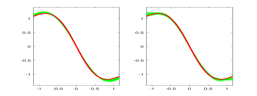
Fig. 2: Example 4. True functions in bold red and beam of 25 estimated drift $b_{4}$ with Hermite (left) and cosine (right) bases, $\rho=0.5$. The MISE$\times 100$ are $0.36$, $0.26$ and the mean of selected dimensions are $4.4$, $6.0$.

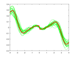
Fig. 3: Example 5. True functions in bold red and beam of 25 estimated drift $b_{5}$ with Hermite basis for $\rho=0$ (left) and $\rho=0.9$ (right). The MISE$\times 100$ are $0.87$, $1.67$ and the mean of selected dimensions are $12.5$ in both cases.

The dependency is contained in the Toeplitz variance matrix $R(\rho):=(\rho^{|i-j|})_{1\leqslant i,j\leqslant N}$ for different values of $\rho$. The choice $\rho=0$ corresponds to the independent case, and we also experiment $\rho=0.5$ (mild dependency) and $\rho=0.9$ (strong correlations). Assumption 3 is not fulfilled but we can consider that the coefficients are in fact null when $|i-j|$ is large enough. The orders of some quantities related to $R(\rho)$ are given in Table 1, and clearly, $\sum_{i,k}R(\rho)_{i,k}/N$ and $\|R(\rho)\|_{\rm op}$ are very close.

	$\rho=0$	$\rho=0.5$	$\rho=0.9$
$N^{-1}\sum_{i,j}R_{i,j}(\rho)$	1	2.96	17.2
$\|R(\rho)\|_{\rm op}$	1	2.99	17.9

Table 1: Order of different quantities associated to the matrix $R(\rho)$.

The penalty term is computed as in Comte and Genon-Catalot [7], by an empirical version which directly takes dependence into account without requiring any information on $R$:

$$\widehat{\rm pen}(m):=\kappa\frac{m}{NT}\|\widehat{\bf\Psi}_{m}^{-1}\widehat{\bf\Psi}_{m,\sigma}\|_{\rm op}\quad{\rm with}\quad\widehat{\bf\Psi}_{m,\sigma}=(\langle\sigma\varphi_{j},\sigma\varphi_{\ell}\rangle_{N})_{j,\ell}$$

and $\kappa=2$ for both bases. Then, the model $\widehat{m}$ is chosen as the minimizer of $-\|\widehat{b}_{m}\|_{N}^{2}+\widehat{\rm pen}(m)$ for $m\leqslant 10$ (resp. $m\leqslant 20$) for the Hermite basis, except in example 5, where we set $m\leqslant 15$ because otherwise the selected dimension was systematically the maximal one (resp. for the cosine basis), such that

$$m\|\widehat{\bf\Psi}_{m}^{-1}\|_{\rm op}^{1/4}\leqslant NT\textrm{ (empirical collection of models)}.$$

We present illustrations of the estimation procedure obtained from simulated paths in Figures 1, 2, 3 for examples 3, 4 and 5. Figures 1 and 2 allow the comparison of the results obtained for Hermite (left pictures) and cosine (right pictures) bases, for $\rho=0.5$. Figure 3 shows the difference of estimation in the Hermite basis when $\rho=0$ (left picture) and when $\rho=0.9$ (right picture). The scenario is the same in the three figures: $N=200$ and $T=100$ (with $1000$ observations with step $\Delta=0.1$ for each path). The MISE over the 25 repetitions are given, together with the mean of the selected dimensions. We can see that the examples are quite different, and that the estimation method works in a convincing way, even for strong dependency ($\rho=0.9$).
We also illustrate on the scenario $N=100$ and $T=100$ (with $1000$ observations with step $\Delta=0.1$) for each path, which was a middle scenario in Comte and Genon-Catalot [7], the influence of the value of $\rho$ on the MISE computed over 200 repetitions: the results are given in Table 2. We see that the MISE increases when $\rho$ increases, slightly from $\rho=0$ to $\rho=0.5$ and much more importantly from $\rho=0.5$ to $\rho=0.9$. On the contrary, the selected dimensions for each basis are rather unchanged in these different cases. This suggests that bias and variance increase simultaneously and proportionally. The Hermite basis gives lower MISEs for examples 1 to 3, and the cosine basis wins for examples 4 and 5.

		$\rho=0$		$\rho=0.5$		$\rho=0.9$
Ex.		Hermite	Cosine	Hermite	Cosine	Hermite	Cosine
Ex.1	MISE	$0.11_{(0.08)}$	$0.80_{(0.24)}$	$0.13_{(0.10)}$	$0.83_{(0.29)}$	$0.63_{(0.54)}$	$1.38_{(6.29)}$
	Dim	$6.2_{(0.8)}$	$6.2_{(1.5)}$	$6.1_{(0.5)}$	$6.2_{(1.5)}$	$6.3_{(1.1)}$	$6.3_{(1.2)}$
Ex.2	MISE	$0.78_{(0.18)}$	$0.95_{(0.19)}$	$0.78_{(0.18)}$	$0.94_{(0.18)}$	$1.02_{(0.47)}$	$1.18_{(0.49)}$
	Dim	$6.1_{(0.5)}$	$10.3_{(1.9)}$	$6.1_{(0.5)}$	$10.4_{(2.0)}$	$6.1_{(0.5)}$	$10.3_{(2.0)}$
Ex.3	MISE	$0.22_{(0.16)}$	$0.34_{(0.11)}$	$0.21_{(0.16)}$	$0.37_{(0.14)}$	$0.44_{(0.41)}$	$0.55_{(0.43)}$
	Dim	$7.8_{(0.7)}$	$4.1_{(0.4)}$	$7.7_{(0.7)}$	$4.1_{(0.4)}$	$7.8_{(0.8)}$	$4.2_{(0.6)}$
Ex.4	MISE	$0.41_{(0.18)}$	$0.35_{(0.15)}$	$0.46_{(0.21)}$	$0.39_{(0.18)}$	$1.06_{(0.66)}$	$1.02_{(0.60)}$
	Dim	$4.4_{(0.8)}$	$5.1_{(1.4)}$	$4.4_{(0.8)}$	$5.2_{(1.3)}$	$4.9_{(1.3)}$	$5.6_{(1.5)}$
Ex. 5	MISE	$1.55_{(0.85)}$	$1.49_{(0.61)}$	$1.81_{(0.97)}$	$1.58_{(0.62)}$	$4.14_{(4.22)}$	$3.15_{(3.55)}$
	Dim	$11.2_{(1.3)}$	$6.3_{(0.8)}$	$11.4_{(1.4)}$	$6.2_{(0.6)}$	$11.5_{(1.5)}$	$6.3_{(0.8)}$

Table 2: 100 MISE (with 100 Std in parenthesis) and mean selected dimensions (with StD in parenthesis) for the examples 1 to 5, $N=100$ and $T=100$, for Hermite and cosine bases and 3 values of $\rho$ (0 for independence, $\rho=0.9$ for strong dependency).

6 Proofs

6.1 Proof of Lemma 1

First of all, let us show that the symmetric matrix $\mathbf{\Psi}_{m,\sigma}$ is nonnegative. Indeed, for every $y\in\mathbb{R}^{m}$,

$$y^{*}\mathbf{\Psi}_{m,\sigma}y = \frac{1}{NT}\sum_{j,\ell=1}^{m}y_{j}y_{\ell}\sum_{i,k=1}^{N}\mathbb{E}\left(\left(\int_{0}^{T}\sigma(X_{s}^{i})\varphi_{j}(X_{s}^{i})dB_{s}^{i}\right)\left(\int_{0}^{T}\sigma(X_{s}^{k})\varphi_{\ell}(X_{s}^{k})dB_{s}^{k}\right)\right)$$

$$= \frac{1}{NT}\mathbb{E}\left[\left(\sum_{i=1}^{N}\int_{0}^{T}\sigma(X_{s}^{i})\tau_{y}(X_{s}^{i})dB_{s}^{i}\right)^{2}\right]\geqslant 0\quad{\rm with}\quad\tau_{y}(.):=\sum_{j=1}^{m}y_{j}\varphi_{j}(.).$$

On the one hand, since $\mathbf{\Psi}_{m,\sigma}$ is a nonnegative matrix, since $d\langle B^{i},B^{k}\rangle_{t}=R_{i,k}dt$ for every $i,k\in\{1,\dots,N\}$, and by the stochastic integration by parts formula,

$${\rm trace}(\mathbf{\Psi}_{m}^{-1}\mathbf{\Psi}_{m,\sigma}) \leqslant \|\mathbf{\Psi}_{m}^{-1}\|_{\rm op}{\rm trace}(\mathbf{\Psi}_{m,\sigma})=\frac{1}{NT}\|\mathbf{\Psi}_{m}^{-1}\|_{\rm op}\sum_{j=1}^{m}\mathbb{E}\left[\left(\sum_{i=1}^{N}\int_{0}^{T}\sigma(X_{s}^{i})\varphi_{j}(X_{s}^{i})dB_{s}^{i}\right)^{2}\right]$$

$$= \frac{1}{NT}\|\mathbf{\Psi}_{m}^{-1}\|_{\rm op}\sum_{j=1}^{m}\sum_{i,k=1}^{N}\int_{0}^{T}R_{i,k}\mathbb{E}(\sigma(X_{s}^{i})\varphi_{j}(X_{s}^{i})\sigma(X_{s}^{k})\varphi_{j}(X_{s}^{k}))ds$$

$$\leqslant \frac{1}{N}\|\mathbf{\Psi}_{m}^{-1}\|_{\rm op}\left(N+\sum_{i\neq k}|R_{i,k}|\right)\sum_{j=1}^{m}\int_{-\infty}^{\infty}\sigma(x)^{2}\varphi_{j}(x)^{2}f_{T}(x)dx$$

$$\leqslant \mathfrak{c}_{1}\|\mathbf{\Psi}_{m}^{-1}\|_{\rm op}L(m)\left(1+\frac{1}{N}\sum_{i\neq k}|R_{i,k}|\right)\quad{\rm with}\quad\mathfrak{c}_{1}=\int_{-\infty}^{\infty}\sigma(x)^{2}f_{T}(x)dx.$$

On the other hand, assume now that $\sigma$ is bounded. Again, since $d\langle B^{i},B^{k}\rangle_{t}=R_{i,k}dt$ for every $i,k\in\{1,\dots,N\}$, and by the stochastic integration by parts formula, for every $y\in\mathbb{R}^{m}$,

$$y^{*}\mathbf{\Psi}_{m,\sigma}y = \frac{1}{NT}\mathbb{E}\left[\left(\sum_{i=1}^{N}\int_{0}^{T}\sigma(X_{s}^{i})\tau_{y}(X_{s}^{i})dB_{s}^{i}\right)^{2}\right]$$ (12)

$$\leqslant \frac{1}{T}\left(1+\frac{1}{N}\sum_{i\neq k}|R_{i,k}|\right)\int_{0}^{T}\mathbb{E}(\sigma(X_{s})^{2}\tau_{y}(X_{s})^{2})ds$$

$$\leqslant \left(1+\frac{1}{N}\sum_{i\neq k}|R_{i,k}|\right)\int_{-\infty}^{\infty}\sigma(x)^{2}\left(\sum_{j=1}^{m}y_{j}\varphi_{j}(x)\right)^{2}f_{T}(x)dx$$

$$\leqslant \|\sigma\|_{\infty}^{2}\left(1+\frac{1}{N}\sum_{i\neq k}|R_{i,k}|\right)\|\mathbf{\Psi}_{m}^{1/2}y\|_{2,m}^{2}.$$

Thus, since $\mathbf{\Psi}_{m,\sigma}$ is nonnegative, and by Inequality (12),

$${\rm trace}(\mathbf{\Psi}_{m}^{-1/2}\mathbf{\Psi}_{m,\sigma}\mathbf{\Psi}_{m}^{-1/2}) \leqslant m\|\mathbf{\Psi}_{m}^{-1/2}\mathbf{\Psi}_{m,\sigma}\mathbf{\Psi}_{m}^{-1/2}\|_{\rm op}$$

$$\hskip 56.9055pt=m\cdot\sup\{y^{*}\mathbf{\Psi}_{m,\sigma}y\textrm{ $;$ }y\in\mathbb{R}^{m}\textrm{ and }\|\mathbf{\Psi}_{m}^{1/2}y\|_{2,m}=1\}$$

$$\leqslant m\|\sigma\|_{\infty}^{2}\left(1+\frac{1}{N}\sum_{i\neq k}|R_{i,k}|\right).$$

6.2 Proof of Theorem 1

The proof of Theorem 1 relies on the two following lemmas.

Lemma 2.

There exists a deterministic constant $\mathfrak{c}_{\ref{bound_variance_remainder}}>0$, not depending on $m$ and $N$, such that

$$\mathbb{E}(|\widehat{\bf E}_{m}^{*}\widehat{\bf E}_{m}|^{2})\leqslant\mathfrak{c}_{\ref{bound_variance_remainder}}\frac{mL(m)^{2}}{N^{2}}\left[1+\left(\frac{1}{N}\sum_{i\not=k}|R_{i,k}|\right)^{2}\right].$$

Lemma 3.

Consider the event

$$\Omega_{m}:=\left\{\sup_{\tau\in\mathcal{S}_{m}}\left|\frac{\|\tau\|_{N}^{2}}{\|\tau\|_{f_{T}}^{2}}-1\right|\leqslant\frac{1}{2}\right\}.$$

Under Assumptions 1, 2 and 3, there exists a deterministic constant $\mathfrak{c}_{\ref{deviation_probabilities}}>0$, not depending on $m$ and $N$, such that

$$\mathbb{P}(\Omega_{m}^{c})\leqslant\frac{\mathfrak{c}_{\ref{deviation_probabilities}}}{N^{6}}\quad\textrm{and}\quad\mathbb{P}(\widehat{\Lambda}_{m}^{c})\leqslant\frac{\mathfrak{c}_{\ref{deviation_probabilities}}}{N^{6}}.$$

6.2.1 Steps of the proof

First of all,

$$\|\widetilde{b}_{m}-b_{I}\|_{N}^{2} = \|b_{I}\|_{N}^{2}\mathbf{1}_{\widehat{\Lambda}_{m}^{c}}+\|\widehat{b}_{m}-b_{I}\|_{N}^{2}\mathbf{1}_{\widehat{\Lambda}_{m}}$$ (13)

$$= U_{1}+U_{2}+U_{3}$$

where $U_{1}:=\|b_{I}\|_{N}^{2}\mathbf{1}_{\widehat{\Lambda}_{m}^{c}}$,

$$U_{2}:=\|\widehat{b}_{m}-b_{I}\|_{N}^{2}\mathbf{1}_{\widehat{\Lambda}_{m}\cap\Omega_{m}}\quad{\rm and}\quad U_{3}:=\|\widehat{b}_{m}-b_{I}\|_{N}^{2}\mathbf{1}_{\widehat{\Lambda}_{m}\cap\Omega_{m}^{c}}.$$

Let us find suitable bounds on $\mathbb{E}(U_{1})$, $\mathbb{E}(U_{2})$ and $\mathbb{E}(U_{3})$.

• Bound on $\mathbb{E}(U_{1})$. By Cauchy-Schwarz’s inequality,

  $$\mathbb{E}(U_{1}) \leqslant \mathbb{E}(\|b_{I}\|_{N}^{4})^{1/2}\mathbb{P}(\widehat{\Lambda}_{m}^{c})^{1/2}\leqslant\mathbb{E}\left(\frac{1}{T}\int_{0}^{T}b_{I}(X_{t})^{4}dt\right)^{1/2}\mathbb{P}(\widehat{\Lambda}_{m}^{c})^{1/2}$$

  $$\leqslant \mathfrak{c}_{1}\mathbb{P}(\widehat{\Lambda}_{m}^{c})^{1/2}<\infty\quad{\rm with}\quad\mathfrak{c}_{1}=\left(\int_{-\infty}^{\infty}b_{I}(x)^{4}f_{T}(x)dx\right)^{1/2}<\infty.$$

• Bound on $\mathbb{E}(U_{2})$. Let $\Pi_{N,m}(.)$ be the orthogonal projection from $\mathbb{L}^{2}(I,f_{T}(x)dx)$ onto $\mathcal{S}_{m}$ with respect to the empirical scalar product $\langle.,.\rangle_{N}$. Then,

  $$\|\widehat{b}_{m}-b_{I}\|_{N}^{2}=\|\widehat{b}_{m}-\Pi_{N,m}(b_{I})\|_{N}^{2}+\min_{\tau\in\mathcal{S}_{m}}\|b_{I}-\tau\|_{N}^{2}.$$ (14)

  As in the proof of Comte and Genon-Catalot [7], Proposition 2.1, on $\Omega_{m}$,

  $$\|\widehat{b}_{m}-\Pi_{N,m}(b_{I})\|_{N}^{2}=\widehat{\bf E}_{m}^{*}\widehat{\bf\Psi}_{m}^{-1}\widehat{\bf E}_{m}\leqslant 2\widehat{\bf E}_{m}^{*}\mathbf{\Psi}_{m}^{-1}\widehat{\bf E}_{m}.$$

  So,

  $$\mathbb{E}(\|\widehat{b}_{m}-\Pi_{N,m}(b_{I})\|_{N}^{2}\mathbf{1}_{\widehat{\Lambda}_{m}\cap\Omega_{m}}) \leqslant 2\mathbb{E}\left(\sum_{j,\ell=1}^{m}[\widehat{\bf E}_{m}]_{j}[\widehat{\bf E}_{m}]_{\ell}\mathbf{\Psi}_{m}^{-1}(j,\ell)\right)$$

  $$= \frac{2}{NT}\sum_{j,\ell=1}^{m}\mathbf{\Psi}_{m,\sigma}(j,\ell)\mathbf{\Psi}_{m}^{-1}(j,\ell)=\frac{2}{NT}{\rm trace}(\mathbf{\Psi}_{m}^{-1}\mathbf{\Psi}_{m,\sigma})$$

  $$= \frac{2}{NT}{\rm trace}(\mathbf{\Psi}_{m}^{-1/2}\mathbf{\Psi}_{m,\sigma}\mathbf{\Psi}_{m}^{-1/2}).$$

  Then, by Equality (14) and Lemma 1,

  $$\mathbb{E}(U_{2}) \leqslant \mathbb{E}\left(\min_{\tau\in\mathcal{S}_{m}}\|b_{I}-\tau\|_{N}^{2}\right)+\frac{2}{NT}{\rm trace}(\mathbf{\Psi}_{m}^{-1/2}\mathbf{\Psi}_{m,\sigma}\mathbf{\Psi}_{m}^{-1/2})$$

  $$\leqslant \min_{\tau\in\mathcal{S}_{m}}\|b_{I}-\tau\|_{f_{T}}^{2}+\frac{2m}{NT}\|\sigma\|_{\infty}^{2}\left(1+\frac{1}{N}\sum_{i\neq k}|R_{i,k}|\right).$$

• Bound on $\mathbb{E}(U_{3})$. By the definition of the event $\widehat{\Lambda}_{m}$ and by Lemma 2,

  $$\mathbb{E}(\|\widehat{b}_{m}-\Pi_{N,m}(b_{I})\|_{N}^{2}\mathbf{1}_{\widehat{\Lambda}_{m}\cap\Omega_{m}^{c}}) = \mathbb{E}[(\widehat{\bf E}_{m}^{*}\widehat{\bf\Psi}_{m}^{-1}\widehat{\bf E}_{m})\mathbf{1}_{\widehat{\Lambda}_{m}\cap\Omega_{m}^{c}}]$$

  $$\hskip 56.9055pt\leqslant\mathbb{E}(\|\widehat{\bf\Psi}_{m}^{-1}\|_{\rm op}|\widehat{\bf E}_{m}^{*}\widehat{\bf E}_{m}|\mathbf{1}_{\widehat{\Lambda}_{m}\cap\Omega_{m}^{c}})$$

  $$\leqslant \frac{\mathfrak{c}_{T}(p)}{L(m)}\cdot\frac{NT}{\log(NT)}\mathbb{E}(|\widehat{\bf E}_{m}^{*}\widehat{\bf E}_{m}|^{2})^{1/2}\mathbb{P}(\Omega_{m}^{c})^{1/2}$$

  $$\leqslant \frac{\mathfrak{c}_{2}m^{1/2}}{\log(NT)}\left(1+\frac{1}{N}\sum_{i\neq k}|R_{i,k}|\right)\mathbb{P}(\Omega_{m}^{c})^{1/2}$$

  where $\mathfrak{c}_{2}>0$ is a deterministic constant not depending on $m$ and $N$. Then,

  $$\mathbb{E}(U_{3}) \leqslant \mathbb{E}(\|\widehat{b}_{m}-\Pi_{N,m}(b_{I})\|_{N}^{2}\mathbf{1}_{\widehat{\Lambda}_{m}\cap\Omega_{m}^{c}})+\mathbb{E}(\|b_{I}\|_{N}^{2}\mathbf{1}_{\widehat{\Lambda}_{m}\cap\Omega_{m}^{c}})$$

  $$\leqslant \frac{\mathfrak{c}_{2}m^{1/2}}{\log(NT)}\left(1+\frac{1}{N}\sum_{i\neq k}|R_{i,k}|\right)\mathbb{P}(\Omega_{m}^{c})^{1/2}+\mathfrak{c}_{1}\mathbb{P}(\Omega_{m}^{c})^{1/2}.$$

So,

$$\mathbb{E}(\|\widetilde{b}_{m}-b_{I}\|_{N}^{2}) \leqslant \min_{\tau\in\mathcal{S}_{m}}\|b_{I}-\tau\|_{f_{T}}^{2}$$

$$\hskip 14.22636pt+\left[\frac{2m}{NT}\|\sigma\|_{\infty}^{2}+\mathfrak{c}_{2}\frac{\sqrt{m\mathbb{P}(\Omega_{m}^{c})}}{\log(NT)}\right]\left(1+\frac{1}{N}\sum_{i\not=k}|R_{i,k}|\right)+\mathfrak{c}_{1}(\mathbb{P}(\widehat{\Lambda}_{m}^{c})^{1/2}+\mathbb{P}(\Omega_{m}^{c})^{1/2}).$$

Therefore, by Lemma 3, there exists a deterministic constant $\mathfrak{c}_{3}>0$, not depending on $m$ and $N$, such that

$$\mathbb{E}(\|\widetilde{b}_{m}-b_{I}\|_{N}^{2})\leqslant\min_{\tau\in\mathcal{S}_{m}}\|b_{I}-\tau\|_{f_{T}}^{2}+\frac{\mathfrak{c}_{3}m}{NT}\left(1+\frac{1}{N}\sum_{i\not=k}|R_{i,k}|\right)+\frac{\mathfrak{c}_{3}}{N}.$$

6.2.2 Proof of Lemma 2

By Jensen’s inequality, by Burkholder-Davis-Gundy’s inequality, and since $d\langle B^{i},B^{k}\rangle_{t}=R_{i,k}dt$ for every $i,k\in\{1,\dots,N\}$, there exists a deterministic constant $\mathfrak{c}_{1}>0$, not depending on $m$ and $N$, such that

$$\mathbb{E}(|\widehat{\bf E}_{m}^{*}\widehat{\bf E}_{m}|^{2}) \leqslant m\sum_{j=1}^{m}\mathbb{E}(\widehat{\bf E}_{m}(j)^{4})\leqslant\frac{\mathfrak{c}_{1}m}{N^{4}T^{4}}\sum_{j=1}^{m}\mathbb{E}\left(\left\langle\sum_{i=1}^{N}\int_{0}^{T}\sigma(X_{s}^{i})\varphi_{j}(X_{s}^{i})dB_{s}^{i}\right\rangle_{T}^{2}\right)$$

$$\leqslant \frac{2\mathfrak{c}_{1}m}{N^{4}T^{4}}\sum_{j=1}^{m}(\mathbb{E}(D_{j}^{2})+\mathbb{E}(A_{j}^{2})),$$

where

$$D_{j}:=\sum_{i=1}^{N}\int_{0}^{T}\sigma(X_{s}^{i})^{2}\varphi_{j}(X_{s}^{i})^{2}ds\quad{\rm and}\quad A_{j}:=\sum_{i\neq k}R_{i,k}\int_{0}^{T}\sigma(X_{s}^{i})\varphi_{j}(X_{s}^{i})\sigma(X_{s}^{k})\varphi_{j}(X_{s}^{k})ds$$

for every $j\in\{1,\dots,m\}$. On the one hand, by Jensen’s inequality,

$$\sum_{j=1}^{m}\mathbb{E}(D_{j}^{2}) \leqslant NT\sum_{j=1}^{m}\sum_{i=1}^{N}\int_{0}^{T}\mathbb{E}(\sigma(X_{s}^{i})^{4}\varphi_{j}(X_{s}^{i})^{4})ds$$

$$\leqslant N^{2}TL(m)^{2}\int_{0}^{T}\mathbb{E}(\sigma(X_{s})^{4})ds=N^{2}T^{2}L(m)^{2}\int_{-\infty}^{\infty}\sigma(x)^{4}f_{T}(x)dx.$$

On the other hand, by Jensen’s inequality and Cauchy-Schwarz’s inequality,

$$\sum_{j=1}^{m}\mathbb{E}(A_{j}^{2}) \leqslant T\left(\sum_{i\not=k}|R_{i,k}|\right)\sum_{j=1}^{m}\sum_{i\neq k}|R_{i,k}|\int_{0}^{T}\mathbb{E}(\sigma(X_{s}^{i})^{2}\varphi_{j}(X_{s}^{i})^{2}\sigma(X_{s}^{k})^{2}\varphi_{j}(X_{s}^{k})^{2})ds$$

$$\leqslant T\left(\sum_{i\not=k}|R_{i,k}|\right)^{2}\sum_{j=1}^{m}\int_{0}^{T}\mathbb{E}(\sigma(X_{s})^{4}\varphi_{j}(X_{s})^{4})ds$$

$$\leqslant T^{2}\left(\sum_{i\not=k}|R_{i,k}|\right)^{2}L(m)^{2}\int_{-\infty}^{\infty}\sigma(x)^{4}f_{T}(x)dx.$$

Therefore,

$$\mathbb{E}(|\widehat{\bf E}_{m}^{*}\widehat{\bf E}_{m}|^{2})\leqslant\frac{\mathfrak{c}_{2}}{N^{2}T^{2}}mL(m)^{2}\left[1+\left(\frac{1}{N}\sum_{i\not=k}|R_{i,k}|\right)^{2}\right]$$

with

$$\mathfrak{c}_{2}=2\mathfrak{c}_{1}\int_{-\infty}^{\infty}\sigma(x)^{4}f_{T}(x)dx.$$

6.2.3 Proof of Lemma 3

Let $(\overline{\varphi}_{1},\dots,\overline{\varphi}_{N_{T}})$ be the orthonormal family of $\mathbb{L}^{2}(I,f_{T}(x)dx)$ derived from $(\varphi_{1},\dots,\varphi_{N_{T}})$ via Gram-Schmidt’s method. Consider also the matrix

$$\widehat{\bf G}_{m}:=\sum_{i=1}^{N}\widehat{\bf G}_{m}(X^{i}),$$

where

$$\widehat{\bf G}_{m}(\psi):=\frac{1}{NT}\left(\int_{0}^{T}\overline{\varphi}_{j}(\psi(t))\overline{\varphi}_{\ell}(\psi(t))dt\right)_{j,\ell\in\{1,\dots,m\}}\textrm{$;$ }\forall\psi\in\Omega.$$

The random matrix $\widehat{\bf G}_{m}(X^{i})$ has the same eigenvalues as $N^{-1}\mathbf{\Psi}_{m}^{-1/2}\widehat{\bf\Psi}_{m}(X^{i})\mathbf{\Psi}_{m}^{-1/2}$, where

$$\widehat{\bf\Psi}_{m}(\psi):=\left(\frac{1}{T}\int_{0}^{T}\varphi_{j}(\psi(t))\varphi_{\ell}(\psi(t))dt\right)_{j,\ell\in\{1,\dots,m\}}\textrm{$;$ }\forall\psi\in\Omega.$$

Moreover, for every $\psi\in\Omega$, by Jensen’s and Cauchy-Schwarz’s inequalities,

$$\|\widehat{\bf\Psi}_{m}(\psi)\|_{\rm op}^{2} = \sup_{\|x\|_{2,m}=1}\sum_{\ell=1}^{m}\left[\frac{1}{T}\int_{0}^{T}\left(\sum_{j=1}^{m}\varphi_{j}(\psi(t))\varphi_{\ell}(\psi(t))x_{j}\right)dt\right]^{2}$$ (15)

$$\leqslant \frac{1}{T}\sup_{\|x\|_{2,m}=1}\sum_{\ell=1}^{m}\int_{0}^{T}\varphi_{\ell}(\psi(t))^{2}\left(\sum_{j=1}^{m}\varphi_{j}(\psi(t))x_{j}\right)^{2}dt$$

$$\leqslant \frac{L(m)}{T}\sup_{\|x\|_{2,m}=1}\int_{0}^{T}\left(\sum_{j=1}^{m}\varphi_{j}(\psi(t))x_{j}\right)^{2}dt\leqslant L(m)^{2}.$$

Notations:

• The semidefinite order on symmetric matrices is denoted by $\preccurlyeq$.

• $\mathbb{E}_{0}(.):=\mathbb{E}(.)$ and $\mathbb{E}_{i}(.):=\mathbb{E}(.|\mathcal{F}_{i})$ for every $i\in\{1,\dots,N\}$.

First of all, note that

$$\|\widehat{\bf G}_{m}-\mathbf{I}\|_{\rm op}\leqslant M_{N}+R_{N},$$

where

$$M_{N}:=\left\|\sum_{i=1}^{N}(\widehat{\bf G}_{m}(X^{i})-\mathbb{E}_{i-1}(\widehat{\bf G}_{m}(X^{i})))\right\|_{\rm op}\quad{\rm and}\quad R_{N}:=\left\|\sum_{i=1}^{N}(\mathbb{E}_{i-1}(\widehat{\bf G}_{m}(X^{i}))-N^{-1}\mathbf{I})\right\|_{\rm op}.$$

The proof of Lemma 3 is dissected in four steps. Step 1 deals with a suitable bound on $\mathbb{P}(M_{N}>\delta/2)$, $\delta>0$, step 2 with a suitable bound on $\mathbb{P}(R_{N}>\delta/2)$,

$$\{\|\mathbf{\Psi}_{m}^{-1}\|_{\rm op}<\|\widehat{\mathbf{\Psi}}_{m}^{-1}-\mathbf{\Psi}_{m}^{-1}\|_{\rm op}\}\subset\Omega_{m}^{c}$$

is established in step 3, and the conclusion comes in step 4.

Step 1. For any $\delta>0$, let us establish a suitable bound on $\mathbb{P}(M_{N}>\delta)$. For every $i\in\{1,\dots,N\}$, since

$$\widetilde{\bf G}_{m}(X^{i}):=\widehat{\bf G}_{m}(X^{i})-\mathbb{E}_{i-1}(\widehat{\bf G}_{m}(X^{i}))$$

is a symmetric matrix, by Jensen’s inequality and by Inequality (15),

$$(-\widetilde{\bf G}_{m}(X^{i}))^{2}=\widetilde{\bf G}_{m}(X^{i})^{2} \preccurlyeq \lambda_{\max}[\widetilde{\bf G}_{m}(X^{i})^{2}]\mathbf{I}$$

$$\hskip 42.67912pt=\|\widehat{\bf G}_{m}(X^{i})-\mathbb{E}_{i-1}(\widehat{\bf G}_{m}(X^{i}))\|_{\rm op}^{2}\mathbf{I}$$

$$\preccurlyeq \frac{2}{N^{2}}(\|\mathbf{\Psi}_{m}^{-1/2}\widehat{\bf\Psi}_{m}(X^{i})\mathbf{\Psi}_{m}^{-1/2}\|_{\rm op}^{2}+\mathbb{E}_{i-1}(\|\mathbf{\Psi}_{m}^{-1/2}\widehat{\bf\Psi}_{m}(X^{i})\mathbf{\Psi}_{m}^{-1/2}\|_{\rm op}^{2}))\mathbf{I}$$

$$\preccurlyeq \frac{2}{N^{2}}(\|\widehat{\bf\Psi}_{m}(X^{i})\|_{\rm op}^{2}+\mathbb{E}_{i-1}(\|\widehat{\bf\Psi}_{m}(X^{i})\|_{\rm op}^{2}))\|{\bf\Psi}_{m}^{-1}\|_{\rm op}^{2}\mathbf{I}\preccurlyeq\mathbf{A}_{i}^{2}$$

with

$$\mathbf{A}_{i}^{2}=\frac{4}{N^{2}}[L(m)(\|{\bf\Psi}_{m}^{-1}\|_{\rm op}\vee 1)]^{2}\mathbf{I}.$$

So, by Azuma’s inequality for matrix martingales (see Tropp [24], Theorem 7.1),

$$\mathbb{P}\left(\lambda_{\max}\left(\sum_{i=1}^{N}\widetilde{\bf G}_{m}(X^{i})\right)>\delta\right)\leqslant m\exp\left(-\frac{\delta^{2}}{8\sigma^{2}}\right)$$

and

$$\mathbb{P}\left(-\lambda_{\min}\left(\sum_{i=1}^{N}\widetilde{\bf G}_{m}(X^{i})\right)>\delta\right)=\mathbb{P}\left(\lambda_{\max}\left(\sum_{i=1}^{N}(-\widetilde{\bf G}_{m}(X^{i}))\right)>\delta\right)\leqslant m\exp\left(-\frac{\delta^{2}}{8\sigma^{2}}\right),$$

where

$$\sigma^{2}=\left\|\sum_{i=1}^{N}\mathbf{A}_{i}^{2}\right\|_{\rm op}=\frac{4}{N}[L(m)(\|{\bf\Psi}_{m}^{-1}\|_{\rm op}\vee 1)]^{2}.$$

This leads to

$$\mathbb{P}(M_{N}>\delta) = \mathbb{P}\left(\left\|\sum_{i=1}^{N}\widetilde{\bf G}_{m}(X^{i})\right\|_{\rm op}>\delta\right)$$

$$\hskip 56.9055pt=\mathbb{P}\left(\max\left\{\lambda_{\max}\left(\sum_{i=1}^{N}\widetilde{\bf G}_{m}(X^{i})\right);-\lambda_{\min}\left(\sum_{i=1}^{N}\widetilde{\bf G}_{m}(X^{i})\right)\right\}>\delta\right)$$

$$\leqslant 2m\exp\left(-\frac{\delta^{2}}{8\sigma^{2}}\right)=2m\exp\left[-\frac{\delta^{2}N}{32[L(m)(\|{\bf\Psi}_{m}^{-1}\|_{\rm op}\vee 1)]^{2}}\right].$$

Step 2. For any $\delta>0$, let us establish a suitable bound on $\mathbb{P}(R_{N}>\delta)$. First of all, let us recall that

$$\mathcal{I}_{N}=\{i\in\{1,\dots,N\}:B^{i}\textrm{ is not independent of }\mathcal{F}_{i-1}\}.$$

For every $i\in\{1,\dots,N\}\backslash\mathcal{I}_{N}$, since $(\overline{\varphi}_{1},\dots,\overline{\varphi}_{N_{T}})$ is an orthonormal family of $\mathbb{L}^{2}(I,f_{T}(x)dx)$,

$$\mathbb{E}_{i-1}(\widehat{\bf G}_{m}(X^{i})) = \mathbb{E}(\widehat{\bf G}_{m}(X))=\left(\frac{1}{NT}\int_{0}^{T}\mathbb{E}(\overline{\varphi}_{j}(X_{t})\overline{\varphi}_{\ell}(X_{t}))dt\right)_{j,\ell}$$

$$= \frac{1}{N}(\langle\overline{\varphi}_{j},\overline{\varphi}_{\ell}\rangle_{f_{T}})_{j,\ell}=\frac{1}{N}\mathbf{I}.$$

Then,

$$R_{N}=\left\|\sum_{i\in\mathcal{I}_{N}}(\mathbb{E}_{i-1}(\widehat{\bf G}_{m}(X^{i}))-N^{-1}\mathbf{I})\right\|_{\rm op}.$$

By Markov’s inequality and Jensen’s inequality (usual and conditional),

$$\mathbb{P}(R_{N}>\delta) \leqslant \frac{\mathbb{E}(R_{N}^{p})}{\delta^{p}}\leqslant\frac{|\mathcal{I}_{N}|^{p-1}}{\delta^{p}}\sum_{i\in\mathcal{I}_{N}}\mathbb{E}(\|\mathbb{E}_{i-1}(\widehat{\bf G}_{m}(X^{i})-N^{-1}\mathbf{I})\|_{\rm op}^{p})$$

$$\leqslant \frac{|\mathcal{I}_{N}|^{p}}{\delta^{p}}\mathbb{E}(\|\widehat{\bf G}_{m}(X)-N^{-1}\mathbf{I}\|_{\rm op}^{p})$$

$$\hskip 85.35826pt=\frac{|\mathcal{I}_{N}|^{p}}{\delta^{p}N^{p}}\mathbb{E}(\|\mathbf{\Psi}_{m}^{-1/2}\widehat{\bf\Psi}_{m}(X)\mathbf{\Psi}_{m}^{-1/2}-\mathbf{I}\|_{\rm op}^{p})$$

$$\leqslant \frac{2^{p-1}|\mathcal{I}_{N}|^{p}}{\delta^{p}N^{p}}[\mathbb{E}(\|\widehat{\bf\Psi}_{m}(X)\|_{\rm op}^{p})\|\mathbf{\Psi}_{m}^{-1}\|_{\rm op}^{p}+1]\leqslant\frac{2^{p}|\mathcal{I}_{N}|^{p}}{\delta^{p}N^{p}}[L(m)(\|\mathbf{\Psi}_{m}^{-1}\|_{\rm op}\vee 1)]^{p}.$$

Step 3. Now, consider

$$\Theta_{m}:=\{\|\mathbf{\Psi}_{m}^{-1}\|_{\rm op}<\|\widehat{\mathbf{\Psi}}_{m}^{-1}-\mathbf{\Psi}_{m}^{-1}\|_{\rm op}\}.$$

Note that

$$\|\widehat{\bf\Psi}_{m}^{-1}-\mathbf{\Psi}_{m}^{-1}\|_{\rm op}=\|\mathbf{\Psi}_{m}^{-\frac{1}{2}}(\widehat{\bf G}_{m}^{-1}-\mathbf{I})\mathbf{\Psi}_{m}^{-\frac{1}{2}}\|_{\rm op}\leqslant\|\widehat{\bf G}_{m}^{-1}-\mathbf{I}\|_{\rm op}\|\mathbf{\Psi}_{m}^{-1}\|_{\rm op}.$$

Moreover, as established in Stewart and Sun [23], for every $\mathbf{A},\mathbf{B}\in\mathcal{M}_{d}(\mathbb{R})$, if $\mathbf{A}$ is invertible and $\|\mathbf{A}^{-1}\mathbf{B}\|_{\rm op}<1$, then $\mathbf{M}:=\mathbf{A}+\mathbf{B}$ is invertible, and

$$\|\mathbf{M}^{-1}-\mathbf{A}^{-1}\|_{\rm op}\leqslant\frac{\|\mathbf{B}\|_{\rm op}\|\mathbf{A}^{-1}\|_{\rm op}^{2}}{1-\|\mathbf{A}^{-1}\mathbf{B}\|_{\rm op}}.$$

On $\Omega_{m}$, by applying this result to $\mathbf{A}=\mathbf{I}$ and $\mathbf{B}=\widehat{\bf G}_{m}-\mathbf{I}$, $\mathbf{A}+\mathbf{B}=\widehat{\bf G}_{m}$ is invertible and

$$\|\widehat{\bf G}_{m}^{-1}-\mathbf{I}\|_{\rm op}\leqslant\frac{\|\widehat{\bf G}_{m}-\mathbf{I}\|_{\rm op}}{1-\|\widehat{\bf G}_{m}-\mathbf{I}\|_{\rm op}}.$$

Therefore,

$$\Theta_{m} \subset \{\|\widehat{\bf G}_{m}^{-1}-\mathbf{I}\|_{\rm op}>1\}\subset\Omega_{m}^{c}\cup(\Omega_{m}\cap\{\|\widehat{\bf G}_{m}^{-1}-\mathbf{I}\|_{\rm op}>1\})$$

$$\subset \Omega_{m}^{c}\cup\left\{\|\widehat{\bf G}_{m}-\mathbf{I}\|_{\rm op}\leqslant\frac{1}{2}\textrm{ and }\frac{\|\widehat{\bf G}_{m}-\mathbf{I}\|_{\rm op}}{1-\|\widehat{\bf G}_{m}-\mathbf{I}\|_{\rm op}}>1\right\}=\Omega_{m}^{c}.$$

Step 4 (conclusion). For any $\delta>0$, the two previous steps leads to

$$\mathbb{P}(\|\widehat{\bf G}_{m}-\mathbf{I}\|_{\rm op}>\delta) \leqslant \mathbb{P}\left(\left\{M_{N}>\frac{\delta}{2}\right\}\cup\left\{R_{N}>\frac{\delta}{2}\right\}\right)$$ (16)

$$\leqslant 2m\exp\left[-\frac{\delta^{2}N}{128[L(m)(\|{\bf\Psi}_{m}^{-1}\|_{\rm op}\vee 1)]^{2}}\right]$$

$$\hskip 113.81102pt+\frac{2^{2p}|\mathcal{I}_{N}|^{p}}{\delta^{p}N^{p}}[L(m)(\|\mathbf{\Psi}_{m}^{-1}\|_{\rm op}\vee 1)]^{p}.$$

As established in the beginning of the proof of Comte and Genon-Catalot [7], Proposition 2.1,

$$\Omega_{m}=\left\{\sup_{\tau\in\mathcal{S}_{m}}\left|\frac{\|\tau\|_{N}^{2}}{\|\tau\|_{f_{T}}^{2}}-1\right|\leqslant\frac{1}{2}\right\}=\left\{\|\widehat{\bf G}_{m}-\mathbf{I}\|_{\rm op}\leqslant\frac{1}{2}\right\}.$$

Then, by Inequality (16), by Assumptions 2 and 3 (leading to (7)), and since $p\geqslant 12$,

$$\mathbb{P}(\Omega_{m}^{c}) \leqslant 2m\exp\left(-\frac{\log(NT)}{256\mathfrak{c}_{T}(p)T}\right)+\frac{2^{3p}(\mathfrak{c}_{T}(p)T)^{p/2}}{2^{p/2}}\cdot\frac{|\mathcal{I}_{N}|^{p}}{N^{p/2}\log(NT)^{p/2}}$$

$$\leqslant \mathfrak{c}_{1}\left(\frac{m}{N^{1+p/2}}+\frac{|\mathcal{I}_{N}|^{p}}{N^{p/2}\log(NT)^{p/2}}\right)\leqslant\frac{\mathfrak{c}_{1}(1+\mathfrak{c}_{\ref{sparsity_condition}}(p))}{N^{6}}$$

where $\mathfrak{c}_{1}>0$ is a deterministic constant not depending on $m$ and $N$. Moreover, on $\widehat{\Lambda}_{m}^{c}$ and by Assumption 2,

$$[L(m)(\|\mathbf{\Psi}_{m}^{-1}\|_{\rm op}\vee 1)]^{2}\leqslant\frac{\mathfrak{c}_{T}(p)}{2}\cdot\frac{NT}{\log(NT)}\quad{\rm and}\quad L(m)(\|\widehat{\bf\Psi}_{m}^{-1}\|_{\rm op}\vee 1)>\mathfrak{c}_{T}(p)\frac{NT}{\log(NT)}.$$

The first inequality implies that

$$L(m)\|\mathbf{\Psi}_{m}^{-1}\|_{\rm op}\leqslant\frac{\mathfrak{c}_{T}(p)}{2}\cdot\frac{NT}{\log(NT)}\quad{\rm and}\quad L(m)\leqslant\frac{\mathfrak{c}_{T}(p)}{2}\cdot\frac{NT}{\log(NT)},$$

and then the second one leads to

$$\mathfrak{c}_{T}(p)\frac{NT}{\log(NT)}<L(m)\|\widehat{\bf\Psi}_{m}^{-1}\|_{\rm op} \leqslant L(m)(\|\widehat{\bf\Psi}_{m}^{-1}-\mathbf{\Psi}_{m}^{-1}\|_{\rm op}+\|\mathbf{\Psi}_{m}^{-1}\|_{\rm op})$$

$$\leqslant L(m)\|\widehat{\bf\Psi}_{m}^{-1}-\mathbf{\Psi}_{m}^{-1}\|_{\rm op}+\frac{\mathfrak{c}_{T}(p)}{2}\cdot\frac{NT}{\log(NT)}.$$

Therefore, by step 3,

$$\mathbb{P}(\widehat{\Lambda}_{m}^{c}) \leqslant \mathbb{P}\left(\frac{\mathfrak{c}_{T}(p)}{2}\cdot\frac{NT}{\log(NT)}\leqslant L(m)\|\widehat{\bf\Psi}_{m}^{-1}-\mathbf{\Psi}_{m}^{-1}\|_{\rm op}\right)$$

$$\leqslant \mathbb{P}(\|\mathbf{\Psi}_{m}^{-1}\|_{\rm op}<\|\widehat{\bf\Psi}_{m}^{-1}-\mathbf{\Psi}_{m}^{-1}\|_{\rm op})\leqslant\mathbb{P}(\Omega_{m}^{c})\leqslant\frac{\mathfrak{c}_{1}(1+\mathfrak{c}_{\ref{sparsity_condition}}(p))}{N^{6}}.$$

6.3 Proof of Theorem 2

Let us consider the events

$$\Omega_{N}:=\bigcap_{m\in\mathcal{M}_{N}^{+}}\Omega_{m}\quad{\rm and}\quad\Xi_{N}:=\{\mathcal{M}_{N}\subset\widehat{\mathcal{M}}_{N}\subset\mathcal{M}_{N}^{+}\},$$

where

$$\mathcal{M}_{N}^{+}:=\left\{m\in\{1,\dots,N_{T}\}:[\mathfrak{c}_{\varphi}^{2}m(\|\mathbf{\Psi}_{m}^{-1}\|_{\rm op}\vee 1)]^{2}\leqslant 4\mathfrak{d}_{T}(p)\frac{NT}{\log(NT)}\right\}.$$

Moreover, recall that

$$\mathcal{M}_{N}=\left\{m\in\{1,\dots,N_{T}\}:[\mathfrak{c}_{\varphi}^{2}m(\|\mathbf{\Psi}_{m}^{-1}\|_{\rm op}\vee 1)]^{2}\leqslant\frac{\mathfrak{d}_{T}(p)}{4}\cdot\frac{NT}{\log(NT)}\right\}\subset\mathcal{M}_{N}^{+}$$

and

$$\widehat{\mathcal{M}}_{N}=\left\{m\in\{1,\dots,N_{T}\}:[\mathfrak{c}_{\varphi}^{2}m(\|\widehat{\bf\Psi}_{m}^{-1}\|_{\rm op}\vee 1)]^{2}\leqslant\mathfrak{d}_{T}(p)\frac{NT}{\log(NT)}\right\}.$$

The proof of Theorem 2 relies on the two following lemmas.

Lemma 4.

Under Assumptions 1, 3 and 4, there exists a deterministic constant $\mathfrak{c}_{\ref{bound_Xi_N}}>0$, not depending on $m$ and $N$, such that

$$\mathbb{P}(\Xi_{N}^{c})\leqslant\frac{\mathfrak{c}_{\ref{bound_Xi_N}}}{N^{5}}.$$

Lemma 5.

Consider the empirical process

$$\nu_{N}(\tau):=\frac{1}{NT}\sum_{i=1}^{N}\int_{0}^{T}\sigma(X_{s}^{i})\tau(X_{s}^{i})dB_{s}^{i}\textrm{ $;$ }\tau\in\mathcal{S}_{1}\cup\dots\cup\mathcal{S}_{N_{T}}.$$

Under Assumptions 1 and 5, there exist deterministic constants $\kappa_{0},\mathfrak{c}_{\ref{bound_empirical_process}}>0$, not depending on $N$, such that $\mathfrak{c}_{\rm cal}\geqslant\kappa_{0}$ and, for every $m\in\mathcal{M}_{N}$,

$$\mathbb{E}\left[\left(\left[\sup_{\tau\in\mathcal{B}_{\widehat{m},m}}|\nu_{N}(\tau)|\right]^{2}-p(\widehat{m},m)\right)_{+}\mathbf{1}_{\Xi_{N}\cap\Omega_{N}}\right]\leqslant\frac{\mathfrak{c}_{\ref{bound_empirical_process}}}{NT}$$

where, for every $m^{\prime}\in\mathcal{M}_{N}$,

$$\mathcal{B}_{m,m^{\prime}}:=\{\tau\in\mathcal{S}_{m\vee m^{\prime}}:\|\tau\|_{f_{T}}=1\}\quad{\rm and}\quad p(m,m^{\prime}):=\frac{\mathfrak{c}_{\rm cal}}{8}\cdot\frac{m\vee m^{\prime}}{NT}\left(1+\frac{1}{N}\sum_{i\neq k}|R_{i,k}|\right).$$

6.3.1 Steps of the proof

First of all,

$$\|\widehat{b}_{\widehat{m}}-b_{I}\|_{N}^{2} = \|\widehat{b}_{\widehat{m}}-b_{I}\|_{N}^{2}\mathbf{1}_{\Xi_{N}^{c}}+\|\widehat{b}_{\widehat{m}}-b_{I}\|_{N}^{2}\mathbf{1}_{\Xi_{N}}$$ (17)

$$=: U_{1}+U_{2}.$$

Let us find suitable bounds on $\mathbb{E}(U_{1})$ and $\mathbb{E}(U_{2})$.

• Bound on $\mathbb{E}(U_{1})$. By the definition of $\widehat{\mathcal{M}}_{N}$ and by Lemma 2,

  $$\mathbb{E}(\|\widehat{b}_{\widehat{m}}-\Pi_{N,\widehat{m}}(b_{I})\|_{N}^{2}\mathbf{1}_{\Xi_{N}^{c}}) = \mathbb{E}[(\widehat{\bf E}_{\widehat{m}}^{*}\widehat{\bf\Psi}_{\widehat{m}}^{-1}\widehat{\bf E}_{\widehat{m}})\mathbf{1}_{\Xi_{N}^{c}}]$$

  $$\hskip 56.9055pt\leqslant\mathbb{E}(\|\widehat{\bf\Psi}_{\widehat{m}}^{-1}\|_{\rm op}|\widehat{\bf E}_{N_{T}}^{*}\widehat{\bf E}_{N_{T}}|\mathbf{1}_{\Xi_{N}^{c}})$$

  $$\leqslant \sqrt{\mathfrak{d}_{T}(p)\frac{NT}{\log(NT)}}\mathbb{E}(|\widehat{\bf E}_{N_{T}}^{*}\widehat{\bf E}_{N_{T}}|^{2})^{1/2}\mathbb{P}(\Xi_{N}^{c})^{1/2}$$

  $$\leqslant \frac{\mathfrak{c}_{1}N}{\log(NT)}\left(1+\frac{1}{N}\sum_{i\neq k}|R_{i,k}|\right)\mathbb{P}(\Xi_{N}^{c})^{1/2}$$

  where $\mathfrak{c}_{1}>0$ is a deterministic constant not depending on $N$. Then,

  $$\mathbb{E}(U_{1}) \leqslant \mathbb{E}(\|\widehat{b}_{\widehat{m}}-\Pi_{N,\widehat{m}}(b_{I})\|_{N}^{2}\mathbf{1}_{\Xi_{N}^{c}})+\mathbb{E}(\|b_{I}\|_{N}^{2}\mathbf{1}_{\Xi_{N}^{c}})$$

  $$\leqslant \frac{\mathfrak{c}_{1}N}{\log(NT)}\left(1+\frac{1}{N}\sum_{i\neq k}|R_{i,k}|\right)\mathbb{P}(\Xi_{N}^{c})^{1/2}+\mathfrak{c}_{2}\mathbb{P}(\Xi_{N}^{c})^{1/2}$$

  with

  $$\mathfrak{c}_{2}=\left(\int_{-\infty}^{\infty}b_{I}(x)^{4}f_{T}(x)dx\right)^{1/2}.$$

  So, by Lemma 3, there exists a deterministic constant $\mathfrak{c}_{3}>0$, not depending on $N$, such that

  $$\mathbb{E}(U_{1})\leqslant\frac{\mathfrak{c}_{3}}{N}\left(1+\frac{1}{N}\sum_{i\neq k}|R_{i,k}|\right).$$

• Bound on $\mathbb{E}(U_{2})$. Note that

  $$U_{2} = \|\widehat{b}_{\widehat{m}}-b_{I}\|_{N}^{2}\mathbf{1}_{\Xi_{N}\cap\Omega_{N}^{c}}+\|\widehat{b}_{\widehat{m}}-b_{I}\|_{N}^{2}\mathbf{1}_{\Xi_{N}\cap\Omega_{N}}$$

  $$=: U_{2,1}+U_{2,2}.$$

  On the one hand, by Lemma 3, there exists a deterministic constant $\mathfrak{c}_{4}>0$, not depending on $N$, such that

  $$\mathbb{P}(\Xi_{N}\cap\Omega_{N}^{c})\leqslant\sum_{m\in\mathcal{M}_{N}^{+}}\mathbb{P}(\Omega_{m}^{c})\leqslant\frac{\mathfrak{c}_{4}}{N^{5}}.$$

  Then, as for $\mathbb{E}(U_{1})$, there exists a deterministic constant $\mathfrak{c}_{5}>0$, not depending on $N$, such that

  $$\mathbb{E}(U_{2,1})\leqslant\frac{\mathfrak{c}_{5}}{N}\left(1+\frac{1}{N}\sum_{i\neq k}|R_{i,k}|\right).$$

  On the other hand,

  $$\gamma_{N}(\tau^{\prime})-\gamma_{N}(\tau)=\|\tau^{\prime}-b\|_{N}^{2}-\|\tau-b\|_{N}^{2}-2\nu_{N}(\tau^{\prime}-\tau)$$

  for every $\tau,\tau^{\prime}\in\mathcal{S}_{1}\cup\dots\cup\mathcal{S}_{N_{T}}$. Moreover, since

  $$\widehat{m}=\arg\min_{m\in\widehat{\mathcal{M}}_{N}}\{-\|\widehat{b}_{m}\|_{N}^{2}+{\rm pen}(m)\}=\arg\min_{m\in\widehat{\mathcal{M}}_{N}}\{\gamma_{N}(\widehat{b}_{m})+{\rm pen}(m)\},$$

  for every $m\in\widehat{\mathcal{M}}_{N}$,

  $$\gamma_{N}(\widehat{b}_{\widehat{m}})+{\rm pen}(\widehat{m})\leqslant\gamma_{N}(\widehat{b}_{m})+{\rm pen}(m).$$ (18)

  On the event $\Xi_{N}=\{\mathcal{M}_{N}\subset\widehat{\mathcal{M}}_{N}\subset\mathcal{M}_{N}^{+}\}$, Inequality (18) remains true for every $m\in\mathcal{M}_{N}$. Then, on $\Xi_{N}$, for any $m\in\mathcal{M}_{N}$, since $\mathcal{S}_{m}+\mathcal{S}_{\widehat{m}}\subset\mathcal{S}_{m\vee\widehat{m}}$ under Assumption 4,

  $$\|\widehat{b}_{\widehat{m}}-b_{I}\|_{N}^{2} \leqslant \|\widehat{b}_{m}-b_{I}\|_{N}^{2}+2\nu_{N}(\widehat{b}_{\widehat{m}}-\widehat{b}_{m})+{\rm pen}(m)-{\rm pen}(\widehat{m})$$

  $$\leqslant \|\widehat{b}_{m}-b_{I}\|_{N}^{2}+\frac{1}{8}\|\widehat{b}_{\widehat{m}}-\widehat{b}_{m}\|_{f_{T}}^{2}$$

  $$\hskip 42.67912pt+8\left(\left[\sup_{\tau\in\mathcal{B}_{m,\widehat{m}}}|\nu_{N}(\tau)|\right]^{2}-p(m,\widehat{m})\right)_{+}+{\rm pen}(m)+8p(m,\widehat{m})-{\rm pen}(\widehat{m}).$$

  Since $\|.\|_{f_{T}}^{2}\mathbf{1}_{\Omega_{N}}\leqslant 2\|.\|_{N}^{2}\mathbf{1}_{\Omega_{N}}$ on $\mathcal{S}_{1}\cup\dots\cup\mathcal{S}_{\max(\mathcal{M}_{N}^{+})}$, and since $8p(m,\widehat{m})\leqslant{\rm pen}(m)+{\rm pen}(\widehat{m})$, on $\Xi_{N}\cap\Omega_{N}$,

  $$\|\widehat{b}_{\widehat{m}}-b_{I}\|_{N}^{2}\leqslant 3\|\widehat{b}_{m}-b_{I}\|_{N}^{2}+4{\rm pen}(m)+16\left(\left[\sup_{\tau\in\mathcal{B}_{m,\widehat{m}}}|\nu_{N}(\tau)|\right]^{2}-p(m,\widehat{m})\right)_{+}.$$

  So, by Lemma 5,

  $$\mathbb{E}(U_{2,2}) \leqslant \min_{m\in\mathcal{M}_{N}}\{\mathbb{E}(3\|\widehat{b}_{m}-b_{I}\|_{N}^{2}\mathbf{1}_{\Xi_{N}})+4{\rm pen}(m)\}+\frac{16\mathfrak{c}_{\ref{bound_empirical_process}}}{NT}$$

  $$\leqslant \mathfrak{c}_{6}\min_{m\in\mathcal{M}_{N}}\left\{\inf_{\tau\in\mathcal{S}_{m}}\|\tau-b_{I}\|_{f_{T}}^{2}+\frac{m}{NT}\left(1+\frac{1}{N}\sum_{i\neq k}|R_{i,k}|\right)\right\}+\frac{\mathfrak{c}_{6}}{N}$$

  where $\mathfrak{c}_{6}>0$ is a deterministic constant not depending on $N$.

6.3.2 Proof of Lemma 4

Note that

$$\Xi_{N}^{c}=\{\mathcal{M}_{N}\not\subset\widehat{\mathcal{M}}_{N}\}\cup\{\widehat{\mathcal{M}}_{N}\not\subset\mathcal{M}_{N}^{+}\}.$$

The proof of Lemma 4 is dissected in three steps. Step 1 deals with a bound on $\mathbb{P}(\mathcal{M}_{N}\not\subset\widehat{\mathcal{M}}_{N})$, step 2 with a bound on $\mathbb{P}(\|\widehat{\bf\Psi}_{m}-\mathbf{\Psi}_{m}\|_{\rm op}>\delta)$, $\delta>0$, and step 3 with a bound on $\mathbb{P}(\widehat{\mathcal{M}}_{N}\not\subset\mathcal{M}_{N}^{+})$.

Step 1. On $\{\mathcal{M}_{N}\not\subset\widehat{\mathcal{M}}_{N}\}$, there exists $m\in\{1,\dots,N_{T}\}$ such that

$$[\mathfrak{c}_{\varphi}^{2}m(\|\mathbf{\Psi}_{m}^{-1}\|_{\rm op}\vee 1)]^{2}\leqslant\frac{\mathfrak{d}_{T}(p)}{4}\cdot\frac{NT}{\log(NT)}\quad{\rm and}\quad[\mathfrak{c}_{\varphi}^{2}m(\|\widehat{\bf\Psi}_{m}^{-1}\|_{\rm op}\vee 1)]^{2}>\mathfrak{d}_{T}(p)\frac{NT}{\log(NT)}.$$

The first inequality is equivalent to

$$\mathfrak{c}_{\varphi}^{4}m^{2}\|\mathbf{\Psi}_{m}^{-1}\|_{\rm op}^{2}\leqslant\frac{\mathfrak{d}_{T}(p)}{4}\cdot\frac{NT}{\log(NT)}\quad{\rm and}\quad\mathfrak{c}_{\varphi}^{4}m^{2}\leqslant\frac{\mathfrak{d}_{T}(p)}{4}\cdot\frac{NT}{\log(NT)},$$

and then the second one leads to

$$\mathfrak{d}_{T}(p)\frac{NT}{\log(NT)}<\mathfrak{c}_{\varphi}^{4}m^{2}\|\widehat{\bf\Psi}_{m}^{-1}\|_{\rm op}^{2} \leqslant 2\mathfrak{c}_{\varphi}^{4}m^{2}(\|\widehat{\bf\Psi}_{m}^{-1}-\mathbf{\Psi}_{m}^{-1}\|_{\rm op}^{2}+\|\mathbf{\Psi}_{m}^{-1}\|_{\rm op}^{2})$$

$$\leqslant 2\mathfrak{c}_{\varphi}^{4}m^{2}\|\widehat{\bf\Psi}_{m}^{-1}-\mathbf{\Psi}_{m}^{-1}\|_{\rm op}^{2}+\frac{\mathfrak{d}_{T}(p)}{2}\cdot\frac{NT}{\log(NT)}.$$

So,

$$\{\mathcal{M}_{N}\not\subset\widehat{\mathcal{M}}_{N}\} \subset \bigcup_{m\in\mathcal{M}_{N}}\left\{\frac{\mathfrak{d}_{T}(p)}{4}\cdot\frac{NT}{\log(NT)}\leqslant\mathfrak{c}_{\varphi}^{4}m^{2}\|\widehat{\bf\Psi}_{m}^{-1}-\mathbf{\Psi}_{m}^{-1}\|_{\rm op}^{2}\right\}$$

$$\subset \bigcup_{m\in\mathcal{M}_{N}}\{\|\mathbf{\Psi}_{m}^{-1}\|_{\rm op}<\|\widehat{\bf\Psi}_{m}^{-1}-\mathbf{\Psi}_{m}^{-1}\|_{\rm op}\}\subset\bigcup_{m\in\mathcal{M}_{N}}\Omega_{m}^{c}$$

and, since $\mathfrak{d}_{T}(p)/4\leqslant\mathfrak{c}_{T}(p)/2$, by Lemma 3,

$$\mathbb{P}(\mathcal{M}_{N}\not\subset\widehat{\mathcal{M}}_{N})\leqslant\sum_{m\in\mathcal{M}_{N}}\mathbb{P}(\Omega_{m}^{c})\leqslant\frac{\mathfrak{c}_{1}}{N^{5}}$$

where $\mathfrak{c}_{1}>0$ is a deterministic constant not depending on $N$.

Step 2. First of all, note that

$$\|\widehat{\bf\Psi}_{m}-\mathbf{\Psi}_{m}\|_{\rm op}\leqslant M_{N}+R_{N},$$

where

$$M_{N}:=\frac{1}{N}\left\|\sum_{i=1}^{N}(\widehat{\bf\Psi}_{m}(X^{i})-\mathbb{E}_{i-1}(\widehat{\bf\Psi}_{m}(X^{i})))\right\|_{\rm op}\textrm{ and }R_{N}:=\frac{1}{N}\left\|\sum_{i=1}^{N}(\mathbb{E}_{i-1}(\widehat{\bf\Psi}_{m}(X^{i}))-\mathbb{E}(\widehat{\bf\Psi}_{m}(X^{i})))\right\|_{\rm op}.$$

On the one hand, for any $\delta>0$, let us establish a suitable bound on $\mathbb{P}(M_{N}>\delta)$. For every $i\in\{1,\dots,N\}$, since

$$\widetilde{\bf\Psi}_{m}(X^{i}):=\frac{1}{N}(\widehat{\bf\Psi}_{m}(X^{i})-\mathbb{E}_{i-1}(\widehat{\bf\Psi}_{m}(X^{i})))$$

is a symmetric matrix, by Jensen’s inequality and by Inequality (15),

$$(-\widetilde{\bf\Psi}_{m}(X^{i}))^{2}=\widetilde{\bf\Psi}_{m}(X^{i})^{2} \preccurlyeq \lambda_{\max}[\widetilde{\bf\Psi}_{m}(X^{i})^{2}]\mathbf{I}=\frac{1}{N^{2}}\|\widehat{\bf\Psi}_{m}(X^{i})-\mathbb{E}_{i-1}(\widehat{\bf\Psi}_{m}(X^{i}))\|_{\rm op}^{2}\mathbf{I}$$

$$\preccurlyeq \frac{2}{N^{2}}(\|\widehat{\bf\Psi}_{m}(X^{i})\|_{\rm op}^{2}+\mathbb{E}_{i-1}(\|\widehat{\bf\Psi}_{m}(X^{i})\|_{\rm op}^{2}))\mathbf{I}\preccurlyeq\mathbf{A}_{i}^{2}$$

with

$$\mathbf{A}_{i}^{2}:=\frac{4L(m)^{2}}{N^{2}}\mathbf{I}.$$

So, by Azuma’s inequality for matrix martingales (see Tropp [24], Theorem 7.1),

$$\mathbb{P}(M_{N}>\delta) = \mathbb{P}\left(\left\|\sum_{i=1}^{N}\widetilde{\bf\Psi}_{m}(X^{i})\right\|_{\rm op}>\delta\right)$$

$$\hskip 56.9055pt=\mathbb{P}\left(\max\left\{\lambda_{\max}\left(\sum_{i=1}^{N}\widetilde{\bf\Psi}_{m}(X^{i})\right);-\lambda_{\min}\left(\sum_{i=1}^{N}\widetilde{\bf\Psi}_{m}(X^{i})\right)\right\}>\delta\right)$$

$$\leqslant 2m\exp\left(-\frac{\delta^{2}N}{32L(m)^{2}}\right).$$

On the other hand, let us establish a suitable bound on $\mathbb{P}(R_{N}>\delta)$. By the definition of $\mathcal{I}_{N}$,

$$R_{N}=\frac{1}{N}\left\|\sum_{i\in\mathcal{I}_{N}}(\mathbb{E}_{i-1}(\widehat{\bf\Psi}_{m}(X^{i}))-\mathbb{E}(\widehat{\bf\Psi}_{m}(X^{i})))\right\|_{\rm op}.$$

Then, by Markov’s inequality and Jensen’s inequality (usual and conditional),

$$\mathbb{P}(R_{N}>\delta) \leqslant \frac{\mathbb{E}(R_{N}^{p})}{\delta^{p}}\leqslant\frac{|\mathcal{I}_{N}|^{p-1}}{\delta^{p}N^{p}}\sum_{i\in\mathcal{I}_{N}}\mathbb{E}[\|\mathbb{E}_{i-1}[\widehat{\bf\Psi}_{m}(X^{i})-\mathbb{E}(\widehat{\bf\Psi}_{m}(X^{i}))]\|_{\rm op}^{p}]$$

$$\leqslant \frac{|\mathcal{I}_{N}|^{p}}{\delta^{p}N^{p}}\mathbb{E}(\|\widehat{\bf\Psi}_{m}(X)-\mathbb{E}(\widehat{\bf\Psi}_{m}(X))\|_{\rm op}^{p})\leqslant\frac{2^{p}|\mathcal{I}_{N}|^{p}}{\delta^{p}N^{p}}L(m)^{p}.$$

Therefore,

$$\mathbb{P}(\|\widehat{\bf\Psi}_{m}-\mathbf{\Psi}_{m}\|_{\rm op}>\delta) \leqslant \mathbb{P}\left(\left\{M_{N}>\frac{\delta}{2}\right\}\cup\left\{R_{N}>\frac{\delta}{2}\right\}\right)$$

$$\leqslant 2m\exp\left(-\frac{\delta^{2}N}{128L(m)^{2}}\right)+\frac{2^{2p}|\mathcal{I}_{N}|^{p}}{\delta^{p}N^{p}}L(m)^{p}.$$

Step 3. On $\{\widehat{\mathcal{M}}_{N}\not\subset\mathcal{M}_{N}^{+}\}$, there exists $m\in\{1,\dots,N_{T}\}$ such that

$$[\mathfrak{c}_{\varphi}^{2}m(\|\widehat{\bf\Psi}_{m}^{-1}\|_{\rm op}\vee 1)]^{2}\leqslant\mathfrak{d}_{T}(p)\frac{NT}{\log(NT)}\quad{\rm and}\quad[\mathfrak{c}_{\varphi}^{2}m(\|\mathbf{\Psi}_{m}^{-1}\|_{\rm op}\vee 1)]^{2}>4\mathfrak{d}_{T}(p)\frac{NT}{\log(NT)}.$$

The first inequality is equivalent to

$$\mathfrak{c}_{\varphi}^{4}m^{2}\|\widehat{\bf\Psi}_{m}^{-1}\|_{\rm op}^{2}\leqslant\mathfrak{d}_{T}(p)\frac{NT}{\log(NT)}\quad{\rm and}\quad\mathfrak{c}_{\varphi}^{4}m^{2}\leqslant\mathfrak{d}_{T}(p)\frac{NT}{\log(NT)},$$

and then the second one leads to

$$4\mathfrak{d}_{T}(p)\frac{NT}{\log(NT)}<\mathfrak{c}_{\varphi}^{4}m^{2}\|\mathbf{\Psi}_{m}^{-1}\|_{\rm op}^{2} \leqslant 2\mathfrak{c}_{\varphi}^{4}m^{2}(\|\mathbf{\Psi}_{m}^{-1}-\widehat{\bf\Psi}_{m}^{-1}\|_{\rm op}^{2}+\|\widehat{\bf\Psi}_{m}^{-1}\|_{\rm op}^{2})$$

$$\leqslant 2\mathfrak{c}_{\varphi}^{4}m^{2}\|\mathbf{\Psi}_{m}^{-1}-\widehat{\bf\Psi}_{m}^{-1}\|_{\rm op}^{2}+2\mathfrak{d}_{T}(p)\frac{NT}{\log(NT)}.$$

Moreover, for every $m\in\{1,\dots,N_{T}\}$,

$$\{\|\mathbf{\Psi}_{m}^{-1}-\widehat{\bf\Psi}_{m}^{-1}\|_{\rm op}>\|\widehat{\bf\Psi}_{m}^{-1}\|_{\rm op}\}$$

$$\hskip 85.35826pt\subset\left\{\|\widehat{\bf\Psi}_{m}^{-1/2}\mathbf{\Psi}_{m}\widehat{\bf\Psi}_{m}^{-1/2}-\mathbf{I}\|_{\rm op}>\frac{1}{2}\right\}\subset\left\{\|\widehat{\bf\Psi}_{m}-\mathbf{\Psi}_{m}\|_{\rm op}>\frac{1}{2}\|\widehat{\bf\Psi}_{m}^{-1}\|_{\rm op}^{-1}\right\}$$

by interchanging $\widehat{\bf\Psi}_{m}$ and $\mathbf{\Psi}_{m}$ in the proof of Comte and Genon-Catalot [6], Proposition 4.(ii). So,

$$\{\widehat{\mathcal{M}}_{N}\not\subset\mathcal{M}_{N}^{+}\} \subset \bigcup_{\mathfrak{c}_{\varphi}^{4}m^{2}\leqslant\mathfrak{d}_{T}(p)NT/\log(NT)}\left\{2\mathfrak{c}_{\varphi}^{4}m^{2}\|\widehat{\bf\Psi}_{m}^{-1}\|_{\rm op}^{2}<2\mathfrak{d}_{T}(p)\frac{NT}{\log(NT)}\leqslant 2\mathfrak{c}_{\varphi}^{4}m^{2}\|\mathbf{\Psi}_{m}^{-1}-\widehat{\bf\Psi}_{m}^{-1}\|_{\rm op}^{2}\right\}$$

$$\subset \bigcup_{\mathfrak{c}_{\varphi}^{4}m^{2}\leqslant\mathfrak{d}_{T}(p)NT/\log(NT)}\left\{\|\widehat{\bf\Psi}_{m}-\mathbf{\Psi}_{m}\|_{\rm op}>\frac{m}{2}\sqrt{\frac{\log(NT)}{\mathfrak{d}_{T}(p)NT}}\right\}$$

and, by the previous step, Assumptions 3 and 4, and since $p\geqslant 12$,

$$\mathbb{P}(\widehat{\mathcal{M}}_{N}\not\subset\mathcal{M}_{N}^{+}) \leqslant \sum_{\mathfrak{c}_{\varphi}^{4}m^{2}\leqslant\mathfrak{d}_{T}(p)NT/\log(NT)}\left(2m\exp\left(-\frac{N}{512L(m)^{2}}\cdot\frac{m^{2}\log(NT)}{\mathfrak{d}_{T}(p)NT}\right)\right.$$

$$\hskip 142.26378pt\left.+\frac{2^{3p}|\mathcal{I}_{N}|^{p}}{N^{p}}\cdot\frac{\mathfrak{d}_{T}(p)^{p/2}(NT)^{p/2}}{m^{p}\log(NT)^{p/2}}L(m)^{p}\right)$$

$$\leqslant \sum_{\mathfrak{c}_{\varphi}^{4}m^{2}\leqslant\mathfrak{d}_{T}(p)NT/\log(NT)}\left(2m\exp\left(-\frac{1}{512\mathfrak{c}_{\varphi}^{4}}\cdot\frac{\log(NT)}{\mathfrak{d}_{T}(p)T}\right)\right.$$

$$\hskip 142.26378pt\left.+\frac{2^{3p}|\mathcal{I}_{N}|^{p}}{N^{p/2}}\cdot\frac{\mathfrak{d}_{T}(p)^{p/2}T^{p/2}}{\log(NT)^{p/2}}\mathfrak{c}_{\varphi}^{2p}\right)$$

$$\leqslant \sum_{\mathfrak{c}_{\varphi}^{4}m^{2}\leqslant\mathfrak{d}_{T}(p)NT/\log(NT)}\left(\frac{2m}{N^{1+p/2}}+\frac{2^{3p}\mathfrak{c}_{\varphi}^{2p}\mathfrak{c}_{\ref{sparsity_condition}}(p)}{N^{6}}\mathfrak{d}_{T}(p)^{p/2}T^{p/2}\right)\leqslant\frac{\mathfrak{c}_{2}}{N^{5}}$$

where $\mathfrak{c}_{2}>0$ is a deterministic constant not depending on $N$.

6.3.3 Proof of Lemma 5

The proof of Lemma 5 is dissected in two steps.

Step 1. Consider $\tau\in\mathcal{S}_{1}\cup\dots\cup\mathcal{S}_{N_{T}}$ and the martingale $(M_{N}(\tau)_{t})_{t\in[0,T]}$ defined by

$$M_{N}(\tau)_{t}:=\sum_{i=1}^{N}\int_{0}^{t}\sigma(X_{s}^{i})\tau(X_{s}^{i})dB_{s}^{i}\textrm{ $;$ }\forall t\in[0,T].$$

Note that $\nu_{N}(\tau)=M_{N}(\tau)_{T}/(NT)$. Since $d\langle B^{i},B^{k}\rangle_{t}=R_{i,k}dt$ for every $i,k\in\{1,\dots,N\}$,

$$\langle M_{N}(\tau)\rangle_{T} = \sum_{i,k=1}^{N}R_{i,k}\int_{0}^{T}\sigma(X_{t}^{i})\sigma(X_{t}^{k})\tau(X_{t}^{i})\tau(X_{t}^{k})dt$$

$$\hskip 85.35826pt=\int_{0}^{T}(\sigma(X_{t}^{i})\tau(X_{t}^{i}))_{i}^{*}\times R\times(\sigma(X_{t}^{i})\tau(X_{t}^{i}))_{i}dt$$

$$\leqslant \|R\|_{\rm op}\int_{0}^{T}\|(\sigma(X_{t}^{i})\tau(X_{t}^{i}))_{1\leqslant i\leqslant N}\|_{2,N}^{2}dt$$

$$\leqslant \|R\|_{\rm op}\|\sigma\|_{\infty}^{2}\int_{0}^{T}\left(\sum_{i=1}^{N}\tau(X_{t}^{i})^{2}\right)dt=NT\|R\|_{\rm op}\|\sigma\|_{\infty}^{2}\|\tau\|_{N}^{2}.$$

Then, by Assumption 5 and Bernstein’s inequality for local martingales (see Revuz and Yor [22], p. 153), for any $\varepsilon,\upsilon>0$,

$$\mathbb{P}(\nu_{N}(\tau)\geqslant\varepsilon,\|\tau\|_{N}^{2}\leqslant\upsilon^{2}) \leqslant \mathbb{P}(M_{N}(\tau)_{T}^{*}\geqslant NT\varepsilon,\langle M_{N}(\tau)\rangle_{T}\leqslant NT\upsilon^{2}\|R\|_{\rm op}\|\sigma\|_{\infty}^{2})$$

$$\leqslant \exp\left(-\frac{NT\varepsilon^{2}}{2\upsilon^{2}\|\sigma\|_{\infty}^{2}\mathfrak{r}}\right)\quad{\rm with}\quad\mathfrak{r}=1+\mathfrak{m}_{\ref{additional_assumption_Brownians}}.$$

Since this bound remains true by replacing $\tau$ by $-\tau$,

$$\mathbb{P}(|\nu_{N}(\tau)|\geqslant\varepsilon,\|\tau\|_{N}^{2}\leqslant\upsilon^{2}) = \mathbb{P}(\nu_{N}(\tau)\geqslant\varepsilon,\|\tau\|_{N}^{2}\leqslant\upsilon^{2})+\mathbb{P}(\nu_{N}(-\tau)\geqslant\varepsilon,\|\tau\|_{N}^{2}\leqslant\upsilon^{2})$$

$$\leqslant 2\exp\left(-\frac{NT\varepsilon^{2}}{2\upsilon^{2}\|\sigma\|_{\infty}^{2}\mathfrak{r}}\right).$$

Step 2. By using the bound of step 1 and by following the pattern of the proof of Baraud et al. [2], Proposition 6.1, the purpose of this step is to find a suitable bound on

$$\mathbb{E}\left[\left(\left[\sup_{\tau\in\mathcal{B}_{m,m^{\prime}}}|\nu_{N}(\tau)|\right]^{2}-p(m,m^{\prime})\right)_{+}\mathbf{1}_{\Xi_{N}\cap\Omega_{N}}\right]\textrm{ $;$ }m,m^{\prime}\in\mathcal{M}_{N}.$$

Consider $\delta_{0}\in(0,1)$ and let $(\delta_{n})_{n\in\mathbb{N}^{*}}$ be the real sequence defined by

$$\delta_{n}:=\delta_{0}2^{-n}\textrm{ $;$ }\forall n\in\mathbb{N}^{*}.$$

Since $\mathcal{S}_{m\vee m^{\prime}}$ is a vector subspace of $\mathbb{L}^{2}(I,f_{T}(x)dx)$ of dimension $m\vee m^{\prime}$, by Lorentz et al. [19], Chapter 15, Proposition 1.3, for any $n\in\mathbb{N}$, there exists $T_{n}\subset\mathcal{B}_{m,m^{\prime}}$ such that $|T_{n}|\leqslant(3/\delta_{n})^{m\vee m^{\prime}}$ and, for any $\tau\in\mathcal{B}_{m,m^{\prime}}$,

$$\exists f_{n}\in T_{n}:\|\tau-f_{n}\|_{f_{T}}\leqslant\delta_{n}.$$

In particular, note that

$$\tau=f_{0}+\sum_{n=1}^{\infty}(f_{n}-f_{n-1}).$$

Then, for any sequence $(\Delta_{n})_{n\in\mathbb{N}}$ of elements of $(0,\infty)$ such that $\Delta=\sum_{n\in\mathbb{N}}\Delta_{n}<\infty$,

$$\left\{\left[\sup_{\tau\in\mathcal{B}_{m,m^{\prime}}}|\nu_{N}(\tau)|\right]^{2}>\Delta^{2}\right\}$$

$$\hskip 56.9055pt=\left\{\exists(f_{n})_{n\in\mathbb{N}}\in\prod_{n=0}^{\infty}T_{n}:|\nu_{N}(f_{0})|+\sum_{n=1}^{\infty}|\nu_{N}(f_{n}-f_{n-1})|>\Delta\right\}$$

$$\hskip 56.9055pt\subset\left\{\exists(f_{n})_{n\in\mathbb{N}}\in\prod_{n=0}^{\infty}T_{n}:|\nu_{N}(f_{0})|>\Delta_{0}\textrm{ or }[\exists n\in\mathbb{N}^{*}:|\nu_{N}(f_{n}-f_{n-1})|>\Delta_{n}]\right\}$$

$$\hskip 56.9055pt\subset\bigcup_{f_{0}\in T_{0}}\{|\nu_{N}(f_{0})|>\Delta_{0}\}\cup\bigcup_{n=1}^{\infty}\bigcup_{(f_{n-1},f_{n})\in\mathbb{T}_{n}}\{|\nu_{N}(f_{n}-f_{n-1})|>\Delta_{n}\}$$

with $\mathbb{T}_{n}=T_{n-1}\times T_{n}$ for every $n\in\mathbb{N}^{*}$. Moreover, $\|f_{0}\|_{f_{T}}^{2}\leqslant 1$,

$$\|f_{n}-f_{n-1}\|_{f_{T}}^{2}\leqslant 2\delta_{n-1}^{2}+2\delta_{n}^{2}=\frac{5}{2}\delta_{n-1}^{2}\textrm{ $;$ }\forall n\in\mathbb{N}^{*},$$

and $\|.\|_{N}^{2}\mathbf{1}_{\Omega_{N}}\leqslant 3/2\|.\|_{f_{T}}^{2}\mathbf{1}_{\Omega_{N}}$ on $\mathcal{S}_{1}\cup\dots\cup\mathcal{S}_{\max(\mathcal{M}_{N}^{+})}$. So, by step 1,

$$\mathbb{P}\left(\left\{\left[\sup_{\tau\in\mathcal{B}_{m,m^{\prime}}}|\nu_{N}(\tau)|\right]^{2}>\Delta^{2}\right\}\cap\Xi_{N}\cap\Omega_{N}\right)$$

$$\hskip 85.35826pt\leqslant 2\sum_{f_{0}\in T_{0}}\exp\left(-\frac{NT\Delta_{0}^{2}}{3\|f_{0}\|_{f_{T}}^{2}\|\sigma\|_{\infty}^{2}\mathfrak{r}}\right)$$

$$\hskip 170.71652pt+2\sum_{n=1}^{\infty}\sum_{(f_{n-1},f_{n})\in\mathbb{T}_{n}}\exp\left(-\frac{NT\Delta_{n}^{2}}{3\|f_{n}-f_{n-1}\|_{f_{T}}^{2}\|\sigma\|_{\infty}^{2}\mathfrak{r}}\right)$$

$$\hskip 85.35826pt\leqslant 2\exp\left(h_{0}-\frac{NT\Delta_{0}^{2}}{3\|\sigma\|_{\infty}^{2}\mathfrak{r}}\right)+2\sum_{n=1}^{\infty}\exp\left(h_{n-1}+h_{n}-\frac{NT\Delta_{n}^{2}}{15/2\delta_{n-1}^{2}\|\sigma\|_{\infty}^{2}\mathfrak{r}}\right)$$ (19)

with $h_{n}=\log(|T_{n}|)$ for every $n\in\mathbb{N}$. Now, let us take $\Delta_{0}$ such that

$$h_{0}-\frac{NT\Delta_{0}^{2}}{3\|\sigma\|_{\infty}^{2}\mathfrak{r}}=-(m\vee m^{\prime}+x)\quad{\rm with}\quad x>0,$$

which leads to

$$\Delta_{0}=\left[\frac{3\|\sigma\|_{\infty}^{2}\mathfrak{r}}{NT}(m\vee m^{\prime}+x+h_{0})\right]^{1/2},$$

and for every $n\in\mathbb{N}^{*}$, let us take $\Delta_{n}$ such that

$$h_{n-1}+h_{n}-\frac{NT\Delta_{n}^{2}}{15/2\delta_{n-1}^{2}\|\sigma\|_{\infty}^{2}\mathfrak{r}}=-(m\vee m^{\prime}+x+n),$$

which leads to

$$\Delta_{n}=\left[\frac{15/2\delta_{n-1}^{2}\|\sigma\|_{\infty}^{2}\mathfrak{r}}{NT}(m\vee m^{\prime}+x+n+h_{n-1}+h_{n})\right]^{1/2}.$$

For this appropriate sequence $(\Delta_{n})_{n\in\mathbb{N}}$,

$$\mathbb{P}\left(\left\{\left[\sup_{\tau\in\mathcal{B}_{m,m^{\prime}}}|\nu_{N}(\tau)|\right]^{2}>\Delta^{2}\right\}\cap\Xi_{N}\cap\Omega_{N}\right)\leqslant 2e^{-x}e^{-(m\vee m^{\prime})}\left(1+\sum_{n=1}^{\infty}e^{-n}\right)\leqslant 3.2e^{-x}e^{-(m\vee m^{\prime})}$$

by Inequality (19), and

$$\Delta^{2} \leqslant \frac{3\|\sigma\|_{\infty}^{2}\mathfrak{r}}{NT}\left[(m\vee m^{\prime}+x)^{1/2}+h_{0}^{1/2}+\sqrt{\frac{5}{2}}\sum_{n=1}^{\infty}\delta_{n-1}[(m\vee m^{\prime}+x)^{1/2}+(n+h_{n-1}+h_{n})^{1/2}]\right]^{2}$$

$$\leqslant \frac{3\|\sigma\|_{\infty}^{2}\mathfrak{r}}{NT}\delta^{(1)}(m\vee m^{\prime}+x)+\frac{3\|\sigma\|_{\infty}^{2}\mathfrak{r}}{NT}\delta^{(2)}\leqslant\frac{3\|\sigma\|_{\infty}^{2}\mathfrak{r}}{NT}(\delta^{(1)}+\delta^{(2)})(m\vee m^{\prime}+x)$$

with

$$\delta^{(1)}=2\left(1+\sqrt{\frac{5}{2}}\sum_{n=1}^{\infty}\delta_{n-1}\right)^{2},$$

$$\hskip 42.67912pt{\rm and}\quad\delta^{(2)}=2\left[h_{0}^{1/2}+\sqrt{\frac{5}{2}}\sum_{n=1}^{\infty}\delta_{n-1}\left(n+N_{T}\left(2\log\left(\frac{3}{\delta_{0}}\right)+(2n-1)\log(2)\right)\right)^{1/2}\right]^{2}$$

because

$$h_{n-1}+h_{n} \leqslant (m\vee m^{\prime})\left(\log\left(\frac{3}{\delta_{n-1}}\right)+\log\left(\frac{3}{\delta_{n}}\right)\right)$$

$$\leqslant N_{T}\left(2\log\left(\frac{3}{\delta_{0}}\right)+(2n-1)\log(2)\right).$$

Then,

$$\mathbb{P}\left(\left[\sup_{\tau\in\mathcal{B}_{m,m^{\prime}}}|\nu_{N}(\tau)|\right]^{2}-\frac{\kappa_{0}}{\mathfrak{c}_{\rm cal}R_{N}}p(m,m^{\prime})>\frac{\kappa_{0}}{NT}x\right)\leqslant 3.2e^{-x}e^{-(m\vee m^{\prime})}$$

with

$$\kappa_{0}=3\|\sigma\|_{\infty}^{2}\mathfrak{r}(\delta^{(1)}+\delta^{(2)})\quad{\rm and}\quad R_{N}=1+\sum_{i\neq k}|R_{i,k}|.$$

So, by taking $\mathfrak{c}_{\rm cal}\geqslant\kappa_{0}>\kappa_{0}/R_{N}$ and $y=\kappa_{0}x/(NT)$,

$$\mathbb{P}\left(\left[\sup_{\tau\in\mathcal{B}_{m,m^{\prime}}}|\nu_{N}(\tau)|\right]^{2}-p(m,m^{\prime})>y\right)\leqslant 3.2e^{-NTy/\kappa_{0}}e^{-(m\vee m^{\prime})}.$$

Therefore,

$$\mathbb{E}\left[\left(\left[\sup_{\tau\in\mathcal{B}_{m,m^{\prime}}}|\nu_{N}(\tau)|\right]^{2}-p(m,m^{\prime})\right)_{+}\right] = \int_{0}^{\infty}\mathbb{P}\left(\left[\sup_{\tau\in\mathcal{B}_{m,m^{\prime}}}|\nu_{N}(\tau)|\right]^{2}-p(m,m^{\prime})>y\right)dy$$

$$\leqslant 3.2\kappa_{0}\frac{e^{-(m\vee m^{\prime})}}{NT}.$$

A union-bound allows to conclude.

References

• [1] Baraud, Y. Model Selection for Regression on a Random Design. ESAIM: Probab. Statist. 6, 127-146, 2002.
• [2] Baraud, Y., Comte, F. and Viennet, G. Model Selection for (Auto-)Regression with Dependent Data. ESAIM: Probab. Statist. 5, 33-49, 2001.
• [3] Belomestny, D., Pilipauskaité, V. and Podolskij, M. Semiparametric Estimation of McKean-Vlasov SDEs. Ann. Inst. H. Poincaré Probab. Statist. 59, 1, 79-96, 2023.
• [4] Bush, N., Hambly, B.M., Haworth, H., Jin, L. and Reisinger, C. Stochastic Evolution Equations in Portfolio Credit Modelling. SIAM J. Financial Math. 2, 627-664, 2011.
• [5] Cohen, A., Davenport, M.A. and Leviatan, D. On the Stability and Accuracy of Least Squares Approximations. Foundations of Computational Mathematics 13, 819-834, 2013.
• [6] Comte, F. and Genon-Catalot, V. Regression Function Estimation as a Partly Inverse Problem. The Annals of the Institute of Statistical Mathematics 72, 4, 1023-1054, 2020.
• [7] Comte, F. and Genon-Catalot, V. Nonparametric Drift Estimation for i.i.d. Paths of Stochastic Differential Equations. The Annals of Statistics 48, 6, 3336-3365, 2020.
• [8] Comte, F. and Genon-Catalot, V. Drift Estimation on Non Compact Support for Diffusion Models. Stochastic Processes and their Applications 134, 174-207, 2021.
• [9] Comte, F. and Genon-Catalot, V. Nonparametric Adaptive Estimation for Interacting Particle Systems. Scandinavian Journal of Statistics (accepted), 2023.
• [10] Comte, F., Genon-Catalot, V. and Rozenholc, Y. Penalized Nonparametric Mean Square Estimation of the Coefficients of Diffusion Processes. Bernoulli 13, 2, 514-543, 2007.
• [11] Comte, F. and Lacour, C. Noncompact Estimation of the Conditional Density from Direct or Noisy Data. Les Annales de l’I.H.P. Probab. Statist. (accepted), 2021.
• [12] Comte, F. and Marie, N. Nonparametric Estimation for I.I.D. Paths of Fractional SDE. Statistical Inference for Stochastic Processes 24, 3, 669-705, 2021.
• [13] Della Maestra, L. and Hoffmann, M. Nonparametric Estimation for Interacting Particle Systems: McKean-Vlasov Models. Probab. Theory Related Fields 182, 551-613, 2022.
• [14] Denis, C., Dion, C. and Martinez, M. A Ridge Estimator of the Drift from Discrete Repeated Observations of the Solutions of a Stochastic Differential Equation. Bernoulli 27, 2675-2713, 2021.
• [15] Denis, C., Dion, C. and Martinez, M. Consistent Procedures for Multiclass Classification of Discrete Diffusion Paths. Scand. J. Stat. 47, 2, 516-554, 2020.
• [16] Duellmann, K, Küll, J. and Kunisch, M. Estimating Asset Correlations from Stock Prices or Default Rates – Which Method is Superior? Journal of Economic Dynamics and Control 34, 2341-2357, 2010.
• [17] Indritz, J. An Inequality for Hermite Polynomials. Proc. Amer. Math. Soc. 12, 981-983, 1961.
• [18] Lacour, C., Massart, P. and Rivoirard, V. Estimator Selection: a New Method with Applications to Kernel Density Estimation. Sankhya 79, 298-335, 2017.
• [19] Lorentz, G., von Golitschek, M. and Makokov, Y. Constructive Approximation, Advanced Problems. Springer, 1996.
• [20] Marie, N. and Rosier, A. Nadaraya-Watson Estimator for I.I.D. Paths of Diffusion Processes. Scand. J. Stat. 50, 2, 589-637, 2023.
• [21] Merton, R. On the Pricing of Corporate Debt: the Risk Structure of Interest Rates. Journal of Finance 34, 449-470, 1974.
• [22] Revuz, D. and Yor, M. Continuous Martingales and Brownian Motion. Springer, Berlin, 1999.
• [23] Stewart, G.W. and Sun, J-G. Matrix Perturbation Theory. Academic Press, 1990.
• [24] Tropp, J.A. User-Friendly Tail Bounds for Sums of Random Matrices. Found. Comput. Math. 12, 389-434, 2012.