Exploring Self-Attention for Crop-type Classification Explainability

Abstract

Automated crop-type classification using Sentinel-2 satellite time series is essential to support agriculture monitoring. Recently, deep learning models based on transformer encoders became a promising approach for crop-type classification. Using explainable machine learning to reveal the inner workings of these models is an important step towards improving stakeholders’ trust and efficient agriculture monitoring.

In this paper, we introduce a novel explainability framework that aims to shed a light on the essential crop disambiguation patterns learned by a state-of-the-art transformer encoder model. More specifically, we process the attention weights of a trained transformer encoder to reveal the critical dates for crop disambiguation and use domain knowledge to uncover the phenological events that support the model performance. We also present a sensitivity analysis approach to understand better the attention capability for revealing crop-specific phenological events.

We report compelling results showing that attention patterns strongly relate to key dates, and consequently, to the critical phenological events for crop-type classification. These findings might be relevant for improving stakeholder trust and optimizing agriculture monitoring processes. Additionally, our sensitivity analysis demonstrates the limitation of attention weights for identifying the important events in the crop phenology as we empirically show that the unveiled phenological events depend on the other crops in the data considered during training.

I Introduction

Monitoring crop fields is a vital task for funding agriculture, and in the European Union (EU), it plays an essential role in the decision process for agricultural subsidization. The authorities verify whether the crop type grown on an agricultural parcel matches the farmer’s declaration and ensure that certain events, such as mowing and harvesting, occur accordingly in the season. In this context, the introduction of the Sentinel missions fostered the development of automated pipelines for efficient crop monitoring based on the freely available Sentinel satellite observations. According to the audit report for the usage of new imaging technologies for monitoring agricultural policies, in 2019 several EU members developed machine learning algorithms that utilize time series of Sentinel observations for crop-type classification and detection of various phenological events [1].

The last years observed a spread use of deep learning models applied to various applications with overwhelming success [2]. More recently, transformers became dominant deep learning architecture on machine learning tasks which involve sequence processing such as language understanding [3] or video action recognition [4]. Similarly, state-of-the-art approaches for crop-type classification using satellite image sequences were proposed using transformer encoder models [5], [6], [7]. Notwithstanding the accurate crop maps produced by these models, their outcomes do not specifically relate to common agricultural knowledge. Therefore, in order to increase expert trust and foster efficient agriculture monitoring, it is essential to unveil the following aspects of the inner workings of these models:

• Key dates for crop-type classification: Sentinel satellites provide observations with very high temporal resolution. However, their spatial resolution can sometimes be insufficient for the automated processing of small agricultural parcels. In order to avoid expensive field visits, the EU Joint Research Centre seeks to acquire time series for small parcels consisting of satellite data from very high spatial resolution [1]. Hence, understanding the relevant dates for crop disambiguation by the transformer encoder can lead to new insights about designing an optimal schedule and, consequently, cost reduction when acquiring very high-resolution satellite data. Moreover, it can also result in a reduced computational cost as the analysis would need to be performed over a smaller satellite time series sample.

• Crop disambiguation patterns: Transformer encoders use raw time series of Sentinel-2 spectral reflectances and perform automated feature engineering during training which disables straightforward understanding of the model decision process. However, for improving trust and enabling broad adoption of such models for agricultural policy making, it is desirable to connect model decisions to common agricultural knowledge [8]. Furthermore, these insights can enable comparison beyond accuracy of the transformer encoder with the previous machine learning approaches that rely on manual engineering of phenological features [9], [10].

We propose to tackle the above aspects by applying a novel explainability framework for analysis of the inner workings of a trained transformer encoder model for crop-type classification. At the core of the transformer encoder is the self-attention mechanism which models the temporal dependencies in the data through the attention weights [11]. The attention weights indicate the other sequence elements a sequence item should attend to create functional, high-level feature representations for the learning task. [5] demonstrated that the attention weights for crop-type classification are sparsely distributed, assigning high importance only to a few observations throughout the year. Hence, our proposed xAI framework is based on the assumption of sparse attention distribution and relates the sparse attention weights to agricultural domain knowledge in order to uncover and interpret the crop disambiguation patterns learned by the model.

In summary, we propose a methodology for improving transformer explainability for crop-type classification with the following main contributions:

• Identification of the revelant key dates throughout the year for crop-type classification based on summarization of the sparse attention weight patterns.

• Discovery of the phenological events relevant for crop disambiguation by relating the attention patterns with domain knowledge about crop phenology.

• Sensitivity analysis to better understand the capabilities of the attention weights for revealing important events in crop phenology.

Our results show that the attention mechanism can unveil the key dates for crop disambiguation where high attention values are assigned to crops showing distinct spectral reflectance features. We further report that those attention patterns point to specific and relevant events in the crop phenology (e.g. harvesting and growing) that are critical for crop disambiguation. Finally, from the sensitivity analysis, we conclude that the attention weights do not reveal all important events in crop phenology. Hence, the discovered phenological events are conditioned on the presence of the other crops in the dataset.

II Related Work

The rising popularity of deep neural networks came together with a negative stamp of black-box modelling, as they usually do not explicitly unveil the mechanisms to justify the predicted outcome. That led to the emergence of explainable machine learning [12], which aims to improve trust in these models by revealing the learned patterns for their inference. A significant class of explainable machine learning methods consists of approaches based on sensitivity analysis [13]. These methods attribute high importance to the input features whose small perturbations cause a significant change in the output score. One of the benchmark methods in this class discovers the salient features by computing the gradient of the output score w.r.t the input [14]. Another popular method is the computation of Occlusion Sensitivity Maps [15], which discover the salient parts of an image by finding patches whose occlusion leads to a decrease in the model performance. Lately, this method also became popular in applications of explainable machine learning in environmental sciences. Particularly, [16] uses occlusion sensitivity maps to discover image pixels to which a trained convolutional neural network assigns high importance for whale identification. [17] presents another method based on the occlusion of activations in the latent space for explaining wilderness characteristics in Sentinel-2 images.

When it comes to explainability of the attention-based architectures such as transformers, a common approach used in the literature is to attribute high relevance to the sequence elements that are highly attended [18, 19]. The interpretation of attention models as a tool for model explanations is questioned in [20]. This analysis builds on the weak correlation between the attention and gradient-based feature importance measures for a trained RNN model and the existence of adversarial attention distributions. [21] propose alternative techniques for evaluating attention explainability which demonstrates that the prior work does not disprove the usage of attention as an explainability tool. [22] shows that inducing sparsity in the attention distribution does not improve some of the benchmarks set in the prior works for attention explainability. The recent approaches presented in [23] and [24] go beyond interpretability solely based on attention weights and generate model explanations by utilizing all components in the transformer architecture.

The explainability of the deep learning architectures that utilize Sentinel time series for vegetation classification is explored in [8]. The authors propose a perturbation method which reveals the date and band importance in a trained BiLSTM model.
The transformer encoder models for crop-type classification are also mainly explained based on the attention weights. [6] illustrates that the different attention heads focus on different portions of the time series. [5] applies the gradient-based method in [14] on local examples to demonstrate that the transformer encoder suppresses the cloudy observations. This model behaviour derives from the sparse attention distribution, which assigns relevance only to a few time points and neglects the cloudy observations. Although these works shed a light on the inner workings of the transformer encoder model, they still do not reveal the key dates and the phenological events used for crop disambiguation nor evaluate the attention weights capability for modelling detailed crop phenology. These aspects are the focus of our explainability framework presented in this paper.

III Methods

III-A Self-Attention Mechanism

The self-attention mechanism [11] creates high-level feature representations for the sequence elements by modelling the temporal dependencies in the data. In the first step, the input sequence $X\in R^{T\times d_{in}}$ is linearly projected into query matrix $Q\in R^{T\times d_{k}}$, key matrix $K\in R^{T\times d_{k}}$ and value matrix $V\in R^{T\times d_{v}}$ with the following operations:

$$Q=X\theta_{Q},\>K=X\theta_{K}\>,\>V=X\theta_{V}$$ (1)

where $T$ is the length of the time series, $d_{in}$ is the input time series embedding dimension, $d_{k}$ is the query and key embedding dimension and $d_{v}$ is the value embedding dimension. The $\theta$ matrices are projection matrices that are optimized jointly with the usual model parameters during the training process. This allows the model to automatically learn task-specific feature representations from the input data.
In the next step, the ”Scaled Dot-Product Attention” operation [11] is utilized which combines keys and queries into attention weights with the following equation:

$$A=\operatorname{softmax}(\frac{QK^{T}}{\sqrt{d_{k}}})$$ (2)

$A\in R^{T\times T}$ is a square matrix containing the attention weights which model the pairwise alignments of the queries and keys in the projected space. The weights are linear coefficients which relate the different positions in the sequence. Concretely, an entry $a_{ij}$ of the matrix $A$ models the influence of the $j$-th sequence element in creating the high-level feature representation $h_{i}$ for the $i$-th sequence element with the following equation:

$$h_{i}=\sum_{j=1}^{T}a_{ij}{\mbox{\boldmath$v_{j}$}}$$ (3)

where $v_{j}$ is the $j$-th row in the value matrix $V$ representing the value embedding for the position $j$.

[11] also introduces the ”Multi-Head Attention” approach which on parallel projects non-overlapping subspaces of the input data into queries, keys and values and then performs the scaled dot-product attention on each projected version. Next, the results of the different attention operations are concatenated. The number of heads in a transformer encoder layer corresponds to the number of different projections on which the scaled dot-product attention operation is applied.

III-B Transformer Encoders

Transformer encoders [11] are deep learning architectures composed of encoder layers that rely on the self-attention mechanism for modelling the temporal dependencies relevant for inference over sequential data. These layers further process the output of the self-attention mechanism through a residual block and a dense layer. It is important to note that before the data is fed into the encoder layers, the transformer first adds positional encoding to the input in order to inform the model about the order of the sequence elements.

IV Explainability Framework

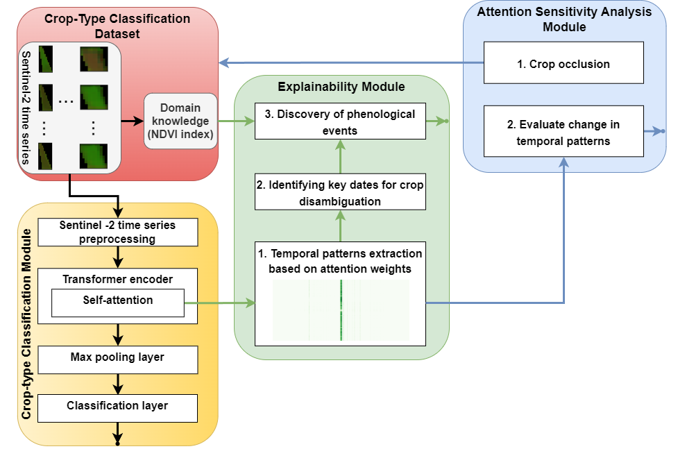
Figure 1: Diagram of the explainability framework presented in this paper. A central component in the proposed framework is the explainability module (depicted in green) that relies on the attention weights of a trained transformer encoder from the crop-type classification module (depicted in yellow). An example attention weights matrix for an agricultural parcel from the crop-type classification dataset is visualized at the bottom of the explainability module. This matrix is typically sparse and assigns high weights only to a few columns (indicated with a dark green colour) which correspond to observations acquired on specific dates in the year. The sparse attention weights are summarized to extract the model temporal patterns and reveal the key dates for crop disambiguation. Finally, these findings are related to NDVI index and raw Sentinel-2 spectral reflectances on the key dates to reveal the critical phenological events that support model predictions. We further introduce the attention sensitivity analysis module (depicted in blue) which tests the attention capability for describing detailed crop phenology by evaluating the sensitivity of the attention patterns to various crop setups in the dataset.

As discussed in Section II, investigating the attention weights learned using self-attention became a popular explainability approach. However, explaining transformer encoder models for crop-type classification based on image sequences remains virtually unexplored, notwithstanding the potential benefits of using attention to identify key dates and reveal the critical phenological events for disambiguation, as highlighted in Section I.

In this paper, we aim to tackle these questions with our proposed explainability framework, visualized in Figure 1, which consists of three core modules: (1) crop-type classification module depicted in the yellow rectangle, (2) explainability module depicted in the green rectangle and (3) attention sensitivity analysis module depicted in the blue rectangle. First, the crop-type classification module trains a transformer encoder model for classifying crop types based on time series of Sentinel-2 observations. Next, the explainability module receives the attention weights from the transformer encoder and derives the temporal patterns and the key dates for crop disambiguation used by the model. These findings are connected to domain knowledge about crop phenology and input time series from the crop-type classification dataset (depicted in the red rectangle) to link learned attention patterns to crop phenology events. Furthermore, we perform a sensitivity analysis of the attention weights based on a crop occlusion to investigate the capability of the attention weights to unambiguously reveal important events in the crop phenology for various crop setups.

IV-A Crop-Type Classification Module

The goal of crop-type classification is to learn a mapping from time series of satellite images acquired over a calendar year for an agricultural parcel to its crop type. For this purpose, we train the transformer encoder model for crop-type classification proposed in [5]. This model first preprocesses the input by adding positional encoding and linearly mapping the sequence embeddings to a higher dimension. Next, the sequence is processed through a series of encoder layers described in Section III-B. The last encoder layer is followed by a max-pooling layer which extracts the highest feature at each time point and a fully connected classification layer that predicts the crop type.

IV-B Domain Knowledge

We introduce agricultural domain knowledge with the NDVI index [25] variable as a proxy which describes crop phenology. It is a measure of the vegetation health and is computed by relating the near-infrared (NIR) band and the visible red (RED) band with the following equation:

$$\text{NDVI}=\frac{\text{NIR}-\text{RED}}{\text{NIR}+\text{RED}}$$ (4)

The NDVI index ranges from -1 to 1. NDVI values between 0.2 and 0.4 usually characterize sparse vegetation patterns. Moderate and dense vegetation are typically characterized by an NDVI index greater than 0.4 [26]. Following the NDVI index’s dynamics over time for an agricultural parcel can reveal important events in the crop lifecycle [27]. In this paper, we analyze the development of the NDVI index over time per crop type to explain the classification patterns and reveal the phenological events relevant to crop disambiguation.

IV-C Explainability Module

The explainability module uses the attention weights from the trained transformer encoder model to reveal the temporal patterns and the key dates for crop disambiguation. These findings are connected to domain knowledge and input time series to explain how attention relates to crop-type classification. Our framework proposes the following three steps to achieve this:

IV-C1 Temporal patterns extraction based on attention weights

As stated in Section III-B, the transformer encoder models the temporal dependencies in the data through the attention mechanism. A typical attention weights matrix for crop-type classification is illustrated at the bottom of this module in Figure 1. It shows sparsely distributed attention weights, with the entire attention being assigned only to a few columns in the matrix. Based on the definition of the self-attention mechanism given in Section III-A, this pattern implies that the new embeddings consist only of the observations acquired on the dates that are highly attended. Therefore, we propose to estimate the importance of date $d$ for classifying agricultural parcel $p$ with the following equation:

$$\alpha_{d_{p}}=\frac{1}{T}\sum_{i=1}^{T}A_{{id}_{p}}$$ (5)

where $T$ is the number of temporal observations for parcel $p$ and $A_{{id}_{p}}$is the attention weight from date $d$ to date $i$ for the parcel $p$. Hence, the importance of date $d$ for parcel $p$ corresponds to the average weight assigned by observation acquired at date $d$ for the high-level feature representations for parcel $p$.

Next, we reveal the importance that the model assigns to date $d$ for disambiguating crop type $c$ with the following equation:

$$\alpha_{d_{c}}=\frac{1}{N_{c}}\sum_{p=1}^{N_{c}}\alpha_{d_{p}}$$ (6)

where $N_{c}$ is the number of agricultural parcels with the crop type $c$ in the test dataset.

IV-C2 Identifying Key Dates for Crop Disambiguation

We further propose to compute the date importance for crop disambiguation with the following equation:

$$\alpha_{d}=\frac{1}{N}\sum_{p=1}^{N}\alpha_{d_{p}}$$ (7)

where $N$ is the total number of field parcels in the test dataset. Consequently, as key dates for crop-type classification, we consider the dates with the highest importance according to this equation.

IV-C3 Discovery of Phenological Events

To unveil the disambiguation patterns learned by the model, we project and visualize the raw spectral reflectances with the Principal Component Analysis (PCA) algorithm and relate the temporal patterns with the average NDVI index per crop type on the identified key dates. To further interpret the phenological events relevant for disambiguating crop types, we relate the temporal patterns over the key dates per agricultural parcel with the input Sentinel-2 observations acquired on the key dates.

IV-D Attention Sensitivity Analysis Module

While the explainability module can identify key dates for crop type classification using attention and connect them to relevant phenological events, we further aim to understand whether the attention patterns are pointing to every relevant phenological event regardless of the crops under consideration or if the transformer encoder model is actually considering only the phenological events relevant for crop disambiguation. The former would imply that the attention weights can be used to describe the crop phenology while the latter would imply that they are optimized only to specific dates relevant for disambiguating the considered crops.

To answer this question, we present an approach that reveals attention sensitivity to the presence of various crop type configurations in the dataset inspired by the occlusion principle described in Section II. First, with crop occlusion, we create new datasets in which one of the crop types from the original dataset is removed. Next, we train a transformer encoder model from scratch on each new dataset and evaluate its attention patterns against the attention patterns in the model trained with the complete set of crops. Concretely, we analyze the change in the importance of date $d$ for classifying crop type $c$ after the occlusion of the crop-type $o$, $\delta_{d_{c,-o}}$, computed with the following equation:

$$\delta_{d_{c,-o}}=\frac{1}{N_{c}}\sum_{p=1}^{N_{c}}(\alpha_{d_{p,-o}}-\alpha_{d_{p}})$$ (8)

where $N_{c}$ is the number of agricultural parcels with the crop type $c$ in the test dataset, $\alpha_{d_{p,-o}}$ is the importance of date $d$ for a parcel $p$ for the model trained on the dataset without crop-type $o$ and $\alpha_{d_{p}}$ is the importance of date $d$ for crop-type $c$ on the model trained with the complete set of crops. Both $\alpha_{d_{p,-o}}$ and $\alpha_{d_{p}}$ are computed with Eq. 5.
The presented sensitivity analysis approach is designed with the following intuition: If attention patterns reveal the important phenological events per crop type, then the temporal importance assigned with the attention mechanism should not change depending on the set of classes under consideration.

V Experimental Setup

V-A Dataset

We performed our experiments on the BavarianCrops dataset, introduced by [5]. The dataset contains agricultural parcels from Bavaria, Germany, represented with the pair $(x,y)$ where:

• $x$ is a time series sequence of observations acquired with Sentinel-2 satellites in the year 2018 for an agricultural parcel [28]. A Sentinel-2 observation is a 13-channel image of an agricultural parcel consisting of the ultra blue channel, the visible RGB channels, visible and near-infrared channels and shortwave infrared channels. The channels encode top-of-atmosphere spectral reflectances [29], and in the dataset, they are further averaged across the image pixels which produces the final input representation $x\in R^{T\times 13}$, where $T$ is the number of observations acquired for an agricultural parcel in 2018. It is worth noting that $T$ can differ across agricultural parcels, ranging from 70 to 144.

• $y$ is the crop-type class grown on an agricultural parcel. The version of the dataset that we are using in the experiments consists of 12 different crop types. The dataset comprises 75683 agricultural parcels and is heavily imbalanced with the grassland crop type being the majority class which is grown on 59% of them. Corn, winter wheat, winter barley and summer barley are grown on 13%, 6%, 6% and 5% of the agricultural parcels, respectively. The rest seven classes cover the remaining 11% of the agricultural parcels in the dataset.

V-B Sentinel-2 Time Series Preprocessing for Explainability Analysis

The input sequences in [5] are reduced to a standard length by randomly sampling 70 observations for every agricultural parcel and a fixed positional encoding is added based on the order in the sampled sequence. These steps hinder the analysis of the attention temporal patterns because one position in the sequence can correspond to observations acquired on different dates, depending on the sampling result. In order to enable explainability of the temporal patterns, we preprocess the input sequences using right padding which adds $\mathrm{𝟎}$ values at the end of the sequence until the maximum number of temporal observations per agricultural parcel is reached. Equally important, we force the model to take the seasonality of the observations into account by replacing the fixed positional encoding with a positional encoding based on the observation acquisition date.

In order to assess whether enabling temporal explainability analysis impacts the model performance, we perform simple hyperparameter tuning for the parameters of the transformer encoder model. We are using the same dataset split, and the training procedure implemented in [5], but employ the focal loss function [30] to tackle class imbalance. .

The classification results for the different sequence aggregation strategies are given on Table I. They are similar to the results reported in [5] and indicate that the proposed preprocessing steps which enable temporal explainability analysis do not negatively impact the model performance. Hence, we perform our next experiments with the model trained on sequences preprocessed with right padding and the configuration of the best model obtained with hyperparameter tuning: 1 encoder layer, 1 head and 128 embedding dimension . We also use a fixed seed for model training to isolate the effect of random initialization of the network parameters and attribute changes derived from class occlusion.

TABLE I: Results for models using positional encoding based on observation acquisition date

Sequence Preprocessing	Accuracy	Class accuracy	F1 score
Right padding	$0.91\pm 0$	$0.62\pm 0.02$	$0.63\pm 0.02$
Random sampling	$0.90\pm 0$	$0.61\pm 0.02$	$0.63\pm 0.02$

VI Attention Explainability Results

VI-A Identifying Attention Temporal Patterns and the Key Dates for Crop Disambiguation

As stated in Section IV-C, we uncover the temporal patterns assigned by the attention weights based on the assumption for sparse attention distribution. Figure 2 reveals the temporal patterns for the most frequent crops in the dataset and it shows that the different crops present distinct attention patterns with high importance being assigned to observations acquired at a few specific dates in a year per crop. Namely, the winter barley crop presents high attention only for the observations acquired at the beginning of July, the corn agricultural parcels are mostly attended based on the observations acquired in late spring and the attention for grassland spreads throughout the spring and summer months. Additionally, the attention for observations acquired outside the spring and summer months in 2018 is typically sparse.

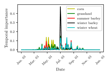
Figure 2: Attention-based temporal importance computed with Eq. 6 for the most frequent crops in the dataset. These attention temporal patterns show that the model assigns high importance to the first days in July for predicting winter barley, to several dates in the Spring for predicting corn and to multiple dates throughout spring and summer for predicting grassland.

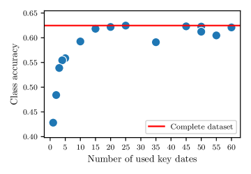
Figure 3: Average class accuracy for the number of key dates used for training the model. The horizontal red line indicates the average class accuracy of the model trained with the complete dataset. This graph shows that using the top few dates with the highest attention averages approximates the accuracy of the model trained on the complete dataset. Detailed confusion matrices for the models trained on top-1, top-3 and top-5 key dates can be seen in appendix Section -D. These results indicate that the approach proposed in Section IV-C2 can be used to identify the key dates in the year for accurate classification.

Further, in section IV-C2, we propose to select the dates with high attention averages as key dates for class disambiguation. To empirically verify this approach, we perform an ablation study that inspects drops in the performance of trained models using the same architecture but only the optimal subset of dates. Concretely:

1. The observation acquisition dates are ranked according to the importance for crop disambiguation computed with Eq. 7.

2. A new dataset is created where the agricultural parcels are represented only by the observations acquired at the top-$t$ dates with the highest importance, $t$ $\in$ $\{1,2,...,T\}$.

3. The transformer encoder model is trained and evaluated on the newly created datasets and the results are compared with the best model using the complete dataset.

The results from our ablation study are shown on Figure 3. As a reference, the accuracy of the model trained on the complete dataset is illustrated with the red horizontal line. This figure illustrates that using only the observations acquired on the top-3 dates with the highest average attention is sufficient for achieving 86% of the accuracy of the reference model which utilizes all available observations. Furthermore, it can be seen that the transformer encoder benefits from adding the observations acquired on the subsequent key dates until the observations acquired on the 15th key date are used, which reaches the accuracy of the original model. However, adding further observations does not improve the classification results. Hence, these results point to the conclusion that the attention weights can identify the key dates throughout the year for accurate crop-type classification.

VI-B Connecting Attention Temporal Patterns to Crop Phenology on the Key Dates for Crop Disambiguation

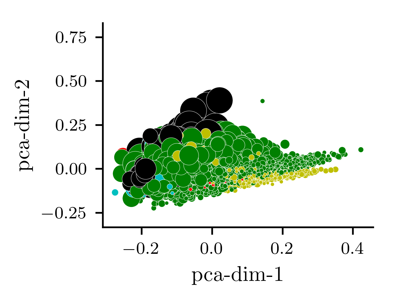
(a) Spectral reflectance on July 01

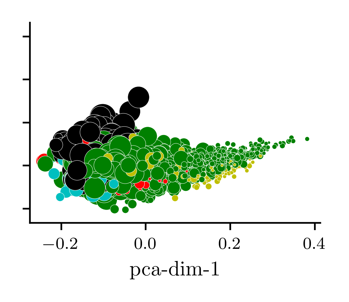
(b) Spectral reflectance on July 03

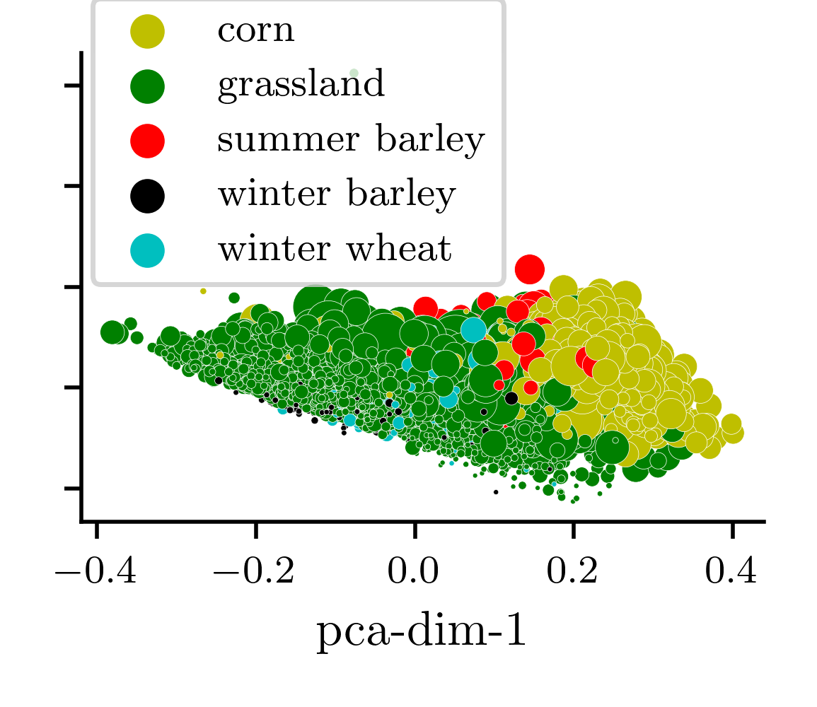
(c) Spectral reflectance on May 07

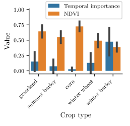
(d) Attention and NDVI on July 01

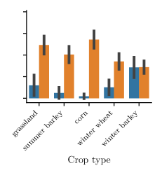
(e) Attention and NDVI on July 03

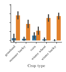
(f) Attention and NDVI on May 07

Figure 4: Overview of attention distribution and spectral characteristics for the top-3 key dates. The first row shows the raw spectral reflectances projected into 2 dimensions with PCA for each date. The size of a point corresponds to the attention importance of the parcel at the given date (Eq. 5). The second row shows the relation between the attention-based temporal importance per crop type (Eq. 7) and the average NDVI per class on these dates. The error bars indicate the standard deviation. These graphs illustrate that the attention mechanism selects the dates on which the crops are discriminative based on their vegetation features. High importance for discrimination is assigned to the crops having distinct phenology that corresponds to sparse vegetation on each key date.

The above results show that the attention weights focus on the key dates in the time series in which the crops can be disambiguated based on the Sentinel-2 reflectances. As stated in Section IV-C3, we further uncover the transformer encoder learned patterns and the critical phenological events for crop disambiguation by relating the attention temporal importance to the raw spectral reflectance and the NDVI index on the key dates for crop disambiguation.
Figure 4 shows the relation between the attention importance and the spectral characteristics on the top-3 dates key dates. The spectral reflectances for July 01 and July 03 visualized in Figures 4a and 4b illustrate that at these dates, attention assigns high importance to a particular subspace of the feature space in which the winter barley and part of the grassland field parcels are located. On the other hand, the parcels showing different spectral properties, such as the corn parcels, are typically located on the other side of the feature space and are not attended. The association between the attention patterns and the crop phenology, visualized in Figures 4d and 4e shows that on these dates, the winter barley parcels have a distinct NDVI index which on average is lower than the NDVI index of the other crops. That indicates that in contrast to the other crops which typically show healthy vegetation, the winter barley crop is characterized by sparse vegetation. Hence, the attention mechanism assigns high importance for efficient class disambiguation to dates where the crops have unique vegetation features. In another example, the spectral reflectances for May 07 (Figure 4c) reveals that attention focuses on an area in the feature space in which typically corn and a subset of grassland agricultural parcels are located. Furthermore, Figure 4f again demonstrates that attention highlights the crop having the most distinct phenology on May 07, as corn is the only crop whose average NDVI index indicates sparse vegetation.

VI-C Discriminative Features - Key Events in Crop Phenology

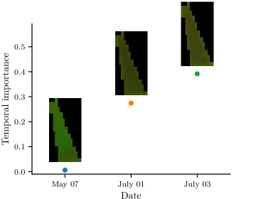
(a) Winter barley parcel

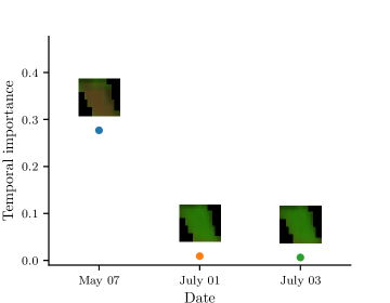
(b) Corn parcel

Figure 5: Sentinel-2 observations and the corresponding temporal importance assigned by the model for two example agricultural parcels during the top-3 dates key dates. The temporal attention importance is calculated with Eq. 5 and is indicated by a dot for each date in the plot. The parcels are visualized with the combination of short-wave infrared (B11), Near Infrared (B8) and the blue band (B2) which highlights healthy vegetation in green and the sparsely vegetated areas and soil in brown [31], [32]. The high importance for the observations acquired in July computed with Eq. 5 indicates that the harvesting event is crucial for winter barley prediction. On the other hand, the high importance of the observation acquired in May on the right plot highlights the importance of the growing event for corn prediction.

With the conclusion that the model discriminates the crops by specific vegetation features shown on certain dates, we propose to further understand the phenological events behind the vegetation features that the model uses for crop disambiguation. In Figure 5, we show examples from the evolvement of winter barley and corn agricultural parcels and the respective attention-based temporal importance on the top-3 key dates. The winter barley example (Figure 5a) presents green observation on May 07, indicating healthy vegetation, which has importance close to zero. On the other hand, the model assigns high importance to observations acquired at beginning of July consisting mostly of brown pixels. Hence, the evolution of this parcel from healthy vegetation in spring to sparse vegetation in July points to the harvesting event and suggests that features displayed around the harvesting time are crucial for winter barley discrimination. The other example for the corn agricultural parcel (Figure 5b) illustrates that the model assigns high attention values to the observation acquired on May 07 which also mostly consists of brown pixels. On the other hand, the observations acquired in July displaying healthy vegetation are not attended. This pattern suggests that the agricultural parcel is classified as corn based on the features shown around the growing time. The interpretation of the above phenological events as harvesting and growing is further strengthened in the appendix by analyzing the dynamics of the NDVI index over time for winter barley and corn shown in figure 11 as well as by the visualization of the highest attended agricultural parcels on the top-3 key dates in figure 12.

In summary, the explainability framework shows that attention weights focus on dates in which crops are separable in the raw spectral reflectance feature space that is used as model input. In addition, the attention highlights features that correspond to important phenological events such as growing or harvesting by which a crop differs from other crops on a given date.

VI-D Attention Sensitivity Analysis

Using our findings that the attention weights guide the transformer encoder model to discriminate the crops based on key phenological events that are unique for a subset of crops on a given date, we further investigate whether the temporal attention patterns per crop type depend on other crops in the dataset. In order to answer this question, we perform the attention sensitivity analysis approach presented in Section IV-D.

Figure 6 visualizes the change in the temporal importance per crop type for the models trained after removing grassland, winter barley and corn agricultural parcels. As shown in Figure 6a, occluding grassland leads to a drastic change in the resulting attention weights for the other crops. For example, the temporal importance for winter barley is shifted from the observations acquired in July (shown in Figure 2) to the observations acquired in late April and May. This implies that the features shown around the harvesting time are not anymore relevant for winter barley discrimination for the model trained on the dataset with the grassland crop removed. Although less symbolic when compared to the grassland occlusion, the attention weights also change after the occlusion of winter barley (Figure 6b) and corn (Figure 6c). Consequently, our analysis shows that the attention weights learn crop disambiguation patterns which do not independently model the behaviour of the individual classes or have a general link to every relevant phenological event. Conversely, the interpretation of the attention weights is always conditional to the classes in the dataset and focuses on events that help to disambiguate them.

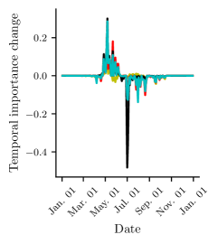
(a) Grassland occlusion

(b) Winter barley occlusion

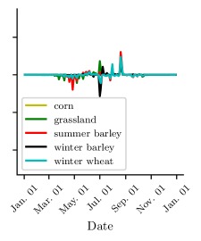
(c) Corn occlusion

Figure 6: Change in attention temporal patterns computed with Eq. 8 after the occlusion of grassland (Figure 6a), winter barley (Figure 6b) and corn (Figure 6c). These plots show that the temporal attention patterns for a crop change depending on the set of crops used in training the model which implies that the phenological events discovered in the explainability module are conditioned on the presence of the other crops in the dataset.

VII Conclusion

In this paper, we presented an explainability framework based on the self-attention mechanism which reveals the key time points and spectral reflectance characteristics for crop-type classification employed by a standard transformer encoder model. First, our framework demonstrates that attention weights reveal a significantly reduced set of key dates throughout the year, yet sufficient for accurate crop-type classification. Next, by relating the attention patterns with agricultural domain knowledge we show that the attention assigns high importance to distinct vegetation features that discriminate the classes at the key dates. Furthermore, by following the evolution of the agricultural parcels over the key dates, we discover that attended features guide the crop discrimination based on important phenological events, such as the harvesting event for winter barley and the growing event for corn. These findings suggest that acquiring observations on a few dates in which the classes show discriminative vegetation features is sufficient for accurate classification and can potentially guide the planning of an optimal schedule for acquiring high-resolution images targetting automated monitoring of small agricultural parcels, thus resulting in smaller costs and faster processing time.

Moreover, as stated in Section I, automated processing of farmer claims requires accurately predicting the crop type and precisely discovering phenological events (e.g. harvesting) for an agricultural parcel. Hence, by analysing the attention patterns learned by the transformer encoder model, our explainability framework enables uncovering the important phenological events for discriminating the classes under consideration. However, from the sensitivity analysis results, we have seen that the detected phenological events are specific for crop disambiguation and are conditioned on the other classes under consideration. Therefore, in future work, we plan to address this limitation by introducing generative modelling for crop-type classification, which will unambiguously reveal the important phenological events per crop type, irrespective of the other crops considered during model training.

[]

Crop-Type Classification Model Selection

-A Training Procedure

The Adam optimization algorithm [33] was used to optimize the transformer encoder models with the following parameters: $beta1=0.9$, $beta2=0.98$, $epsilon=1e-09$, $learning\_rate=0.003$ and $weight\_decay=0.000413$. The learning rate was adapted during the course of the training with the same procedure as described in [11]. In order to tackle the class imbalance problem, we minimized the focal loss function [30] during training. We used the dataset split into training, validation and test set provided in [5]. The models were trained for a maximum of 100 iterations on the training set with an early stopping criterion that evaluates the loss score on the validation set after every 5 training epochs. The classification results are reported on the test set which is not used during the training process. In order to take into account the class imbalance when analysing the classification results, the reported accuracy corresponds to the average of the accuracy of each crop in the dataset.

-B Hyperparameter Tuning Results

In addition to the random sampling and right padding approaches for sequence aggregation described in the experiments Section, we also evaluate the weekly average sequence aggregation approach. This approach averages the input observations for a field parcel acquired within a calendar week. As such, it enables explainability analysis on the attention weights temporal patterns because each position in the preprocessed sequence unambiguously maps to a single calendar week.

We perform simple hyperparameter tuning for the purpose of finding configuration of the transformer encoder which optimally aligns with the introduced sequence preprocessing approaches. Concretely, the following hyperparameters of the model were evaluated for every sequence aggregation approach:

• Positional encoding: observation acquisition date (obs. acq) and sequence order (seq. ord.).

• Number of encoder layers: $[1,2,3,4]$.

• Number of attention heads: $[1,2,4]$.

• Embedding dimension: $[64,128]$.

We used random seed for initialization of the transformer encoder parameters when training the model with every of the above hyperparameter configurations. Additionally, in order to account for the induced randomness in the aggregation by sampling, we train the model five different times for every hyperparameter configuration for the random sampling approach.

Figure 7 demonstrates the impact of the sequence preprocessing on the crop-type classification results. As can be seen from this figure, the right padding and random sampling approaches produce similar results with the right padding approach having higher classification scores on average. Also, it is interesting to note the higher variance of the models obtained with the random sampling approach which is likely caused by the randomness induced by the sampling procedure. These figure also shows that both, right padding and random sampling significantly outperform the weekly average approach.

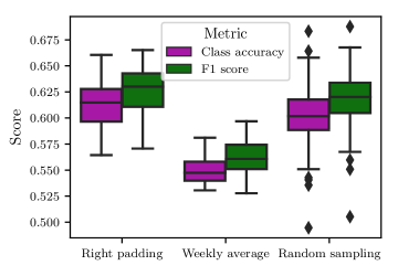
Figure 7: Impact of sequence aggregation approaches on crop-type classification results. The right padding and random sampling approaches lead to better classification results than the weekly average aggregation approach.

Tables II and III display the top-5 hyperparameter configurations for the right padding and random sampling sequence aggregation approaches, respectively. These results illustrate that the different hyperparameter configurations result in similar model performance. Furthermore, they demonstrate that forcing the model to take the seasonality of the observations into account through the positional encoding based on observation acquisition date does not decrease the classification performance.

TABLE II: Top 5 results sorted according to F1 score for the right padding sequence aggregation approach.

Pos. enc	Layers	Heads	Emb. dim	F1 score
obs. acq.	1	1	128	0.67
seq. ord.	1	1	128	0.67
obs. acq.	3	1	128	0.67
obs. acq.	2	1	128	0.66
obs. acq.	2	2	128	0.66

TABLE III: Top-5 results sorted according to F1 score for the random sampling sequence aggregation approach. The reported results are average of the 5 runs for each hyperparameter configuration.

Pos. enc	Layers	Heads	Emb. dim	F1 score
obs. acq.	2	2	64	0.64
obs. acq.	1	4	128	0.64
obs. acq.	2	4	128	0.63
obs. acq.	2	1	128	0.63
obs. acq.	3	1	128	0.63

Detailed Crop-Type Classification Results

The detailed classification results of the different models used in the attention explainability analysis are provided in Table IV.

TABLE IV: Summary of the classification results for the different models used in the proposed explainability framework. The results are reported on the respective test set for each dataset.

Dataset	F1 score	Class accuracy
Entire Dataset	0.64	0.62
Top-1 key date	0.43	0.44
Top-3 key dates	0.54	0.55
Top-5 key dates	0.56	0.57
Grassland occlusion	0.67	0.66
Winter Barley occlusion	0.59	0.58
Corn occlusion	0.62	0.60

-C Classification Results of the Model used for Explainability Analysis

The transformer encoder model used for understanding the utilization of the temporal observations as well as revealing the learned disambiguation patterns was trained with the best configuration found from the hyperparameter tuning (right padding, positional encoding based on the observation acquisition date, 1 layer, 1 head and 128 embedding dimension) and by setting a fixed seed of 0. This model on the test set produces class accuracy of 0.62 and F1 score of 0.64, as shown in the first row of Table IV. The resulting confusion matrix is displayed on Figure 8. Taking into account the crop frequency given in Section V-A, this matrix shows that the model learns to correctly predict the most frequent crops in the data and some of the less frequent crops such as rapeseed. Low accuracy results can be observed for the other less frequent crops in the data.

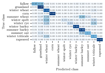
Figure 8: Confusion matrix of the transformer encoder model trained with the best hyperparameter combination and a fixed seed of 0. The model learns to predict with high accuracy the most frequent crops in the dataset as well as some of the less common crops like rapeseed. Low accuracy results occur for less frequent classes which are typically misclassified for some of the more frequent classes.

-D Key Dates Classification Results

The confusion matrices of the models trained on the datasets consisting of top-1, top-3 and top-5 key dates are given in Figure 9. The key dates are calculated according to the approach described in Section IV-C2. Figure 9a shows that the first key date allows the transformer encoder model to learn to discriminate grassland, corn and winter barley with high accuracy. On the other hand, the low frequent classes have typically poor accuracy results. Adding the next two key dates enables the transformer encoder to substantially increase the classification accuracy for summer barley, the winter crops as well as for some low frequent classes such as rapeseed (figure 9b). Using the top-5 key dates (figure 9c) further improves the classification accuracy for the majority of the crops in the dataset.

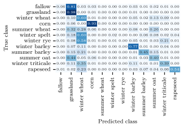
(a) Top-1 key date

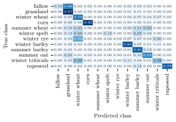
(b) Top-3 key dates

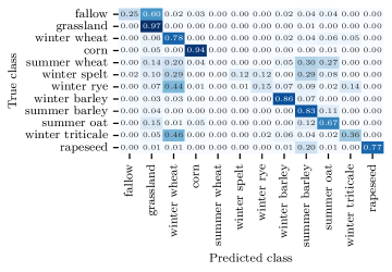
(c) Top-5 key dates

Figure 9: Confusion matrices of the models in the ablation study in section VI-A evaluating the approach for key date selection based on the attention weights. They demonstrate that the model can predict the most frequent crops with high accuracy by using only the top-3 key dates throughout the year. Adding the next two key dates helps to train a model having increased accuracy on the winter wheat crop and some of the less common crops such as fallow.

-E Classification Results after Class Occlusion

The last 3 rows in Table IV show the classification results on the remaining classes after the occlusion of grassland, corn and winter barley, respectively. In comparison with the overall accuracy of the model trained on the entire dataset that is used for discovering the crop-type classification patterns, the occlusion of the grassland parcels leads to better overall discrimination for the remaining crops. On the other hand, the occlusion of the corn and winter barley parcels leads to a decrease in the overall accuracy of the remaining crops.

In order to understand the influence of the crop occlusion on the accuracy of the remaining crops, in Figure 10 we visualize the change in the classification accuracy of the individual crops for the models trained on the datasets resulting after crop occlusion. Concretely, Figure 10a shows that occluding grassland leads to a drastic increase in the accuracy of some of the less frequent crops such as fallow (35%) or summer oat (28%). At the same time, it also leads to a 16% decrease in accuracy for summer barley which is one of the most frequent crops in the data. Hence, these results point out that the large magnitude of change in the attention weights patterns after the grassland occlusion (shown in Figure 6a) directly impacts the accuracy for some of the remaining crops. Furthermore, Figure 10b shows that occluding the winter barley most significantly impacts the classification results of the other winter crops whereas the corn occlusion has little impact in the classification results for the other crops (figure 10c).

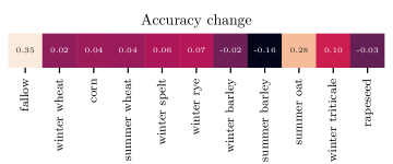
(a) Grassland occlusion

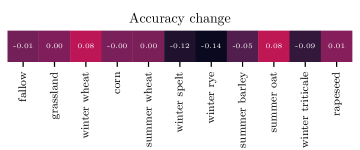
(b) Winter barley occlusion

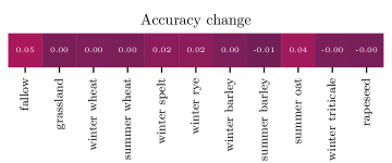
(c) Corn occlusion

Figure 10: Change in the accuracy of the models trained after crop occlusion with the procedure described in Section IV-D. The reported change is equal to the difference between the crop accuracy for the model trained on the occluded dataset and the crop accuracy for the model trained on the entire dataset. The removal of grassland leads to a high change in the accuracy of fallow, summer oat and summer barley. On the other hand, the removal of winter barley mostly impacts the accuracy of the winter crops whereas corn removal has only a slight impact on the accuracy of the other crops.

Agricultural Domain Knowledge

-F NDVI index for Understanding the Crop Phenology

As mentioned in Section IV-B, we use NDVI index as a proxy for understanding the crop phenology. The NDVI temporal dynamics visualized in Figure 11 illustrate the different crop phenologies. For example, the winter crops are characterized by an earlier peak in dense vegetation in Spring and afterwards by sparser vegetation at the beginning of July which indicates the harvesting event for these crops. This is in contrast to corn whose NDVI index points to growth in May and harvesting in September. Summer barley has similar phenology as corn with the distinction that grows earlier and is harvested earlier than corn. On the other hand, grassland phenology is characterized by dense vegetation throughout the entire year.

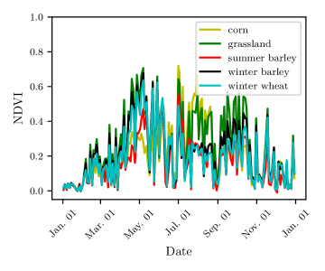
Figure 11: Average NDVI index over time for the 5 most frequent crops in the dataset. The NDVI index describes the phenology of the winter crops by an earlier growth and earlier harvest compared to corn and summer barley phenology which grow later and are harvested at later points in the year. The grassland crop displays distinct phenology from the other crops as it typically shows dense vegetation throughout the entire year.

Highest Attended Parcels on the Key Dates for Crop-Classification

Figure 12 shows that the four parcels with highest attention according to Eq. 5 on the top-3 key dates for crop-type classification are consisting mostly of brown pixels. Based on the observed crop phenology, the highest attended parcels shown in this figure further confirm the finding that the harvesting features displayed on July 01 and July 03 and the growing feature displayed on May 07 are critical for crop disambiguation.

(a) July 01

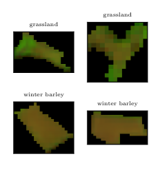
(b) July 03

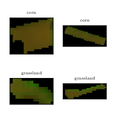
(c) May 07

Figure 12: The 4 highest attended parcels and their respective crop type on the top-3 key dates. As in Figure 5, the parcels are visualized with the combination of short-wave infrared (B11), Near Infrared (B8) and the blue band (B2). The highest attended parcels on these dates mostly consist of brown pixels which indicates the relevance of the harvesting event on July 01 and July 03 and the relevance of the growing event on May 07 for crop disambiguation.

References

- [1] “Using new imaging technologies to monitor the common agricultural policy: steady progress overall, but slower for climate and environment monitoring,” https://op.europa.eu/webpub/eca/special-reports/new-tech-in-agri-monitoring-4-2020/en/, accessed: 2022-08-17.
- [2] Y. LeCun, Y. Bengio, and G. Hinton, “Deep learning,” nature, vol. 521, no. 7553, pp. 436–444, 2015.
- [3] J. Devlin, M.-W. Chang, K. Lee, and K. Toutanova, “Bert: Pre-training of deep bidirectional transformers for language understanding,” arXiv preprint arXiv:1810.04805, 2018.
- [4] R. Girdhar, J. Carreira, C. Doersch, and A. Zisserman, “Video action transformer network,” in Proceedings of the IEEE/CVF Conference on Computer Vision and Pattern Recognition, 2019, pp. 244–253.
- [5] M. Rußwurm and M. Körner, “Self-attention for raw optical satellite time series classification,” ISPRS Journal of Photogrammetry and Remote Sensing, vol. 169, pp. 421–435, 2020. [Online]. Available: https://www.sciencedirect.com/science/article/pii/S0924271620301647
- [6] V. S. F. Garnot, L. Landrieu, S. Giordano, and N. Chehata, “Satellite image time series classification with pixel-set encoders and temporal self-attention,” in Proceedings of the IEEE/CVF Conference on Computer Vision and Pattern Recognition, 2020, pp. 12 325–12 334.
- [7] V. S. F. Garnot and L. Landrieu, “Lightweight temporal self-attention for classifying satellite images time series,” in International Workshop on Advanced Analytics and Learning on Temporal Data. Springer, 2020, pp. 171–181.
- [8] M. Campos-Taberner, F. J. García-Haro, B. Martínez, E. Izquierdo-Verdiguier, C. Atzberger, G. Camps-Valls, and M. A. Gilabert, “Understanding deep learning in land use classification based on sentinel-2 time series,” Scientific reports, vol. 10, no. 1, pp. 1–12, 2020.
- [9] B. D. Wardlow, S. L. Egbert, and J. H. Kastens, “Analysis of time-series modis 250 m vegetation index data for crop classification in the us central great plains,” Remote sensing of environment, vol. 108, no. 3, pp. 290–310, 2007.
- [10] M. Singha, B. Wu, and M. Zhang, “An object-based paddy rice classification using multi-spectral data and crop phenology in assam, northeast india,” Remote Sensing, vol. 8, no. 6, p. 479, 2016.
- [11] A. Vaswani, N. Shazeer, N. Parmar, J. Uszkoreit, L. Jones, A. N. Gomez, Ł. Kaiser, and I. Polosukhin, “Attention is all you need,” in Advances in neural information processing systems, 2017, pp. 5998–6008.
- [12] C. Molnar, Interpretable Machine Learning, 2019, https://christophm.github.io/interpretable-ml-book/.
- [13] N. Xie, G. Ras, M. van Gerven, and D. Doran, “Explainable deep learning: A field guide for the uninitiated,” arXiv preprint arXiv:2004.14545, 2020.
- [14] K. Simonyan, A. Vedaldi, and A. Zisserman, “Deep inside convolutional networks: Visualising image classification models and saliency maps,” in In Workshop at International Conference on Learning Representations. Citeseer, 2014.
- [15] M. D. Zeiler and R. Fergus, “Visualizing and understanding convolutional networks,” in European conference on computer vision. Springer, 2014, pp. 818–833.
- [16] J. Kierdorf, J. Garcke, J. Behley, T. Cheeseman, and R. Roscher, “What identifies a whale by its fluke? on the benefit of interpretable machine learning for whale identification.” ISPRS Annals of Photogrammetry, Remote Sensing & Spatial Information Sciences, vol. 5, no. 2, 2020.
- [17] T. T. Stomberg, T. Stone, J. Leonhardt, and R. Roscher, “Exploring wilderness using explainable machine learning in satellite imagery,” arXiv preprint arXiv:2203.00379, 2022.
- [18] L. Meng, B. Zhao, B. Chang, G. Huang, W. Sun, F. Tung, and L. Sigal, “Interpretable spatio-temporal attention for video action recognition,” in Proceedings of the IEEE/CVF International Conference on Computer Vision Workshops, 2019, pp. 0–0.
- [19] Y. Wang, M. Huang, X. Zhu, and L. Zhao, “Attention-based lstm for aspect-level sentiment classification,” in Proceedings of the 2016 conference on empirical methods in natural language processing, 2016, pp. 606–615.
- [20] S. Jain and B. C. Wallace, “Attention is not Explanation,” in Proceedings of the 2019 Conference of the North American Chapter of the Association for Computational Linguistics: Human Language Technologies, Volume 1 (Long and Short Papers). Minneapolis, Minnesota: Association for Computational Linguistics, Jun. 2019, pp. 3543–3556. [Online]. Available: https://aclanthology.org/N19-1357
- [21] S. Serrano and N. A. Smith, “Is attention interpretable?” in Proceedings of the 57th Annual Meeting of the Association for Computational Linguistics. Florence, Italy: Association for Computational Linguistics, Jul. 2019, pp. 2931–2951. [Online]. Available: https://aclanthology.org/P19-1282
- [22] C. Meister, S. Lazov, I. Augenstein, and R. Cotterell, “Is sparse attention more interpretable?” arXiv preprint arXiv:2106.01087, 2021.
- [23] H. Chefer, S. Gur, and L. Wolf, “Transformer interpretability beyond attention visualization,” in Proceedings of the IEEE/CVF Conference on Computer Vision and Pattern Recognition, 2021, pp. 782–791.
- [24] A. Ali, T. Schnake, O. Eberle, G. Montavon, K.-R. Müller, and L. Wolf, “Xai for transformers: better explanations through conservative propagation,” arXiv preprint arXiv:2202.07304, 2022.
- [25] J. Weier and D. Herring, “Measuring vegetation (ndvi & evi). nasa earth observatory,” Washington, DC, USA, 2000.
- [26] “Ndvi faq: All you need to know about index,” https://eos.com/blog/ndvi-faq-all-you-need-to-know-about-ndvi/, accessed: 2022-08-09.
- [27] Z. Pan, J. Huang, Q. Zhou, L. Wang, Y. Cheng, H. Zhang, G. A. Blackburn, J. Yan, and J. Liu, “Mapping crop phenology using ndvi time-series derived from hj-1 a/b data,” International Journal of Applied Earth Observation and Geoinformation, vol. 34, pp. 188–197, 2015.
- [28] “Sentinel-2,” https://sentinel.esa.int/web/sentinel/missions/sentinel-2, accessed: 2022-01-11.
- [29] “Sentinel-2 l1c,” https://docs.sentinel-hub.com/api/latest/data/sentinel-2-l1c/, accessed: 2022-01-11.
- [30] T.-Y. Lin, P. Goyal, R. Girshick, K. He, and P. Dollár, “Focal loss for dense object detection,” in Proceedings of the IEEE international conference on computer vision, 2017, pp. 2980–2988.
- [31] “Sentinel 2 bands and combinations,” https://gisgeography.com/sentinel-2-bands-combinations/, accessed: 2022-08-09.
- [32] “Landsat 8 (agriculture),” https://www.arcgis.com/home/item.html?id=4f9fb4c44401443b9b416ae7a2917032, accessed: 2022-08-09.
- [33] D. P. Kingma and J. Ba, “Adam: A method for stochastic optimization,” arXiv preprint arXiv:1412.6980, 2014.
[]