Algorithms for geometrical operations with NURBS surfaces.
Abstract
The aim of the paper is to show algorithms for geometrical manipulations on NURBS surfaces. These include generating NURBS surfaces that pass through given points, calculating the minimum distance to a point and include line to surface and surface to surface intersections.
keywords:
NURBS, Isogeometric analysis1 Introduction
Nonuniform rational B-splines or NURBS have been used by the Computer Aided Design (CAD) community for decades. The reason for this is that they are very suitable for defining geometrical shapes and for geometrical operations. A great number of publications on NURBS exist, here we quote the NURBS book [8] and a paper [5] that give a good summary. With the publication of the book Isogeometric Analysis [4] it was suggested that NURBS would also benefit numerical simulation methods such as the Finite Element (FEM)and Boundary Element method (BEM). This was followed by a number of papers discussing the implementation, for example ([6, 1, 3, 10, 7, 9]). A book on the implementation of isogeometric methods into BEM simulation programs was published [2].
A proper implementation of NURBS into FEM and BEM programs, however required revisiting of some geometrical operations. While the CAD community is mainly interested in the graphical display of geometry, the simulation community is interested in generating an ’analysis suitable’ geometry, i.e. one that allows a suitable volume or boundary discretisation. In this paper we concentrate of surfaces, as they are used in BEM, and present algorithms for some geometrical operations. It should be noted that CAD programs have very sophisticated algorithms for computing surface to surface intersections. However, these algorithms produce data that are not ’analysis suitable’.
2 B-splines and NURBS
B-splines are an attractive alternative to Lagrange polynomials and Serendipity functions predominantly used in simulation. The basis for creating the functions is the knot vector. This is a vector containing a series of non-decreasing values of the local coordinate :
| (1) |
A B-spline basis function of order (constant) is given by:
| (2) |
Higher order basis functions are defined by referencing lower order functions:
| (3) |
B-spines are associate with anchors. The location of the -th anchor in the parameter space can be computed by:
| (4) |
Nonuniform rational B-splines or NURBS are based on B-splines but have improved properties for the definition of geometry. NURBS of order are defined as:
| (5) |
where is the number of basis functions and are weights. This can be extended to two dimensions using a tensor product:
| (6) |
where is a NURBS of order in direction.
The coordinates of a point on a curve with the local coordinate can be computed by:
| (7) |
where are NURBS basis functions defined in equation 5 except that numbering starts at 1 instead of 0. are control point coordinates. The vector tangential in direction can be computed by:
| (8) |
The coordinates of a point on a surface with the local coordinate can be computed by:
| (9) |
where are NURBS basis functions defined in equation 6, except that numbering starts at 1 instead of 0. The basis functions are numbered consecutively with a single index instead of two indices and . For a surface the vector in direction can be additionally computed by:
| (10) |
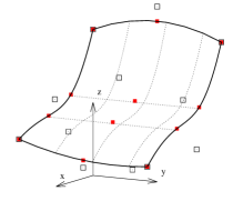
As an example we show in Figure 1 a surface created with the knot vectors:
| (12) | |||||
| (14) |
i.e. quadratic in -direction and linear in direction. The control point coordinates and weights are shown in table 1.
| x | y | z | w | ||
|---|---|---|---|---|---|
| 0 | 0 | 0 | 1 | 0 | 1 |
| 1 | 0 | 0 | 1 | 1 | 0.707 |
| 2 | 0 | 0 | 0 | 1 | 1 |
| 0 | 1 | 1 | 1 | 0 | 1 |
| 1 | 1 | 1 | 1 | 1 | 0.707 |
| 2 | 1 | 1 | 0 | 1 | 1 |
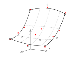
2.1 Trimming
We can cut off a portion of the surface by a process called trimming. We first define the limits of the trimmed space using basis functions and and control points . We then map from a space to a local space:
| (15) |
Finally we map form the coordinate system to the coordinate system using equation (9). In Figure 2 we show an example on how the surface shown in Figure 1 can be trimmed.
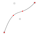
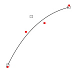
3 Generating NURBS curves and surfaces through a set of points
We can determine the NURBS parameters in such a way that the defined curve or surface either exactly goes through a number of points with the coordinates or is a least square approximation.
First we gather all coordinates of the given points in vector and of the unknown control point coordinates in vector :
| (16) |
For a curve the matrix is given for example by:
| (18) |
We can solve for the control point coordinates by:
| (19) |
where ’’ denotes either a solution by inverting or a least square approximation of depending on the number of points. If the number of points is equal to the number of control points then the curve/surface will go exactly through the specified points.
4 Calculating the closest distance between a point and a surface
To calculate the closest distance of a point to a surface we use an iterative technique. We start with a point on the surface and compute the vector to the specified point. Using dot products with vectors and we estimate increments in the local coordinates. We iterate until the distance from the specified point to the surface does not change. For surfaces which are very curved we need to limit the increments to a maximum value using a damping coefficient (about 0.5 to 0.75) otherwise the iteration may diverge.
5 Intersection between a line and a surface
To calculate the intersection of a line with a surface we also use an iterative process. We define the line with a one dimensional NURBS and compute a vector representing the line. We define as the local coordinate along the line. Starting with which corresponds to the end of (global coordinate ) we compute the closest point to the surface as . We then compute and increment of by projecting this point normal to the line, arriving at a new point on the line closer to the surface. We repeat this process until is very small, i.e. the point on the line corresponds to a point on the surface. We explain the procedure in Figure 6.
Algorithm 3 outlines the steps.
6 Intersection between a surface and a surface
As explained earlier CAD programs have sophisticated and fast intersection algorithms. However, they don’t lead to analysis suitable data. Here we present a simple algorithm that can be used to generate a suitable Boundary element mesh. We explain the determination of the intersection between 2 surfaces on an example involving the surface defined in section 1 and a vertical cylinder depicted in Figure 7.
We specify the cylinder (surface 1) as the intersecting surface and the other surface as the intersected surface (surface 2). Next we subdivide surface 1 in direction and generate vertical lines as shown in Figure 8 left. The number of lines will determine the quality of the intersection curve. We use algorithm 3 to compute the intersection points with surface 2. Next we use algorithm 1 to compute the parameters of a trimming curve that passes through the calculated points. We then trim surface 1 as shown in Figure 8 right.
Remark:
These trimming curve parameters can also be taken from data produced by CAD programs.
To produce analysis suitable data the next steps are more involved. We perform these steps in the local coordinate system of surface 2. First we divide surface 2 into 4 subsurfaces as shown in Figure 9 left. For each subsurface we determine trimming curves that go through the computed intersection points and then trim the subsurfaces (Figure 9 middle). We finally map to global coordinates(Figure 9 right).
Algorithm 4 summarises the steps
7 Summary
In this short paper some algorithms were presented that the author has used to implement isogeometric methods into a BEM simulation program. It is hoped that it will be of benefit to developers of simulation software.
References
- Bazilevs et al. [2010] Bazilevs, Y.; Calo, V.M.; Cottrell, J.A.; Evans, J.A.; Hughes, T.J.R.; Lipton, S.; Scott, M.A.; Sederberg, T.W., Isogeometric analysis using T-splines, Computer Methods in Applied Mechanics and Engineering, 199(5–8):229–263, 2010.
- Beer et al. [2019] Beer, G.; Marussig, B.; Duenser, C. The isogeometric Boundary Element method, volume 90 of Lecture Notes in Applied and Computational Mechanics. Springer Nature, 2019.
- Borden et al. [2011] Borden, M.J.; Scott, M.A.; Evans, J.A.; Hughes, T.J.R., Isogeometric finite element data structures based on Bézier extraction of NURBS, International Journal for Numerical Methods in Engineering, 87(1-5):15–47, 2011.
- Cottrell et al. [2009] Cottrell, J.A.; Hughes, T.J.R.; Bazilevs, Y. Isogeometric Analysis: Toward Integration of CAD and FEA. J. Wiley, 2009.
- Dimas and Briassoulis [1999] Dimas, E.; Briassoulis, D., 3d geometric modelling based on nurbs: a review, Advances in Engineering Software, 30(9):741–751, 1999.
- Hughes et al. [2005] Hughes, T.J.R.; Cottrell, J.A.; Bazilevs, Y., Isogeometric analysis: CAD, finite elements, NURBS, exact geometry and mesh refinement, Computer Methods in Applied Mechanics and Engineering, 194(39–41):4135–4195, October 2005.
- Peake et al. [2013] Peake, M.J.; Trevelyan, J.; Coates, G., Extended isogeometric boundary element method (XIBEM) for two-dimensional Helmholtz problems, Computer Methods in Applied Mechanics and Engineering, 259:93–102, 2013.
- Piegl and Tiller [1997] Piegl, L.; Tiller, W. The NURBS book. Springer-Verlag New York, Inc., New York, NY, USA, 2 edition, 1997.
- Scott et al. [2013] Scott, M.A.; Simpson, R.N.; Evans, J.A.; Lipton, S.; Bordas, S.P.A.; Hughes, T.J.R.; Sederberg, T.W., Isogeometric boundary element analysis using unstructured T-splines, Computer Methods in Applied Mechanics and Engineering, 254:197–221, 2013.
- Simpson et al. [2012] Simpson, R.N.; Bordas, S.P.; Trevelyan, J.; Rabczuk, T., A two-dimensional isogeometric boundary element method for elastostatic analysis, Computer Methods in Applied Mechanics and Engineering, 209:87–100, 2012.