Fractional Order Runge-Kutta Methods

Abstract

This paper investigates, a new class of fractional order Runge-Kutta (FORK) methods for numerical approximation to the solution of fractional differential equations (FDEs). By using the Caputo generalized Taylor formula for Caputo fractional derivative, we construct explicit and implicit FORK methods, as the well-known Runge-Kutta schemes for ordinary differential equations. In the proposed method, due to the dependence of fractional derivatives to a fixed base point $t_{0}$, we had to modify the right-hand side of the given equation in all steps of the FORK methods. Some coefficients for explicit and implicit FORK schemes are presented. The convergence analysis of the proposed method is also discussed. Numerical experiments clarify the effectiveness and robustness of the method..

$\bf{Keywords}$ Fractional differential equations; Caputo fractional derivative; Convergence analysis; Consistency; Stability analysis.

MSC2010: 26A33; 41A25; 65L03.

1 Introduction

In recent years, the numerical approximation for the solutions of FDEs has attracted increasing attention in many fields of applied sciences and engineering [1, 2, 3]. It is common for FDEs to be used in formulating many problems in applied mathematics. Developing numerical methods for fractional differential problems is necessary and important because analytic solutions are usually challenging to obtain. Moreover, it is necessary to develop numerical methods that are highly accurate and easy to use.

It is well known that fractional derivatives have different definitions; the most common and important ones in applications are the Riemann–Liouville and Caputo fractional derivatives. Models describing physical phenomena usually prefer the use of the Caputo derivative. One of the reasons is that the Riemann–Liouville derivative needs initial conditions containing the limit values of the Rieman–Liouville fractional derivative at the origin of time. In contrast, the initial conditions for Caputo derivatives are the same as for integer-order differential equations. Therefore, using the Caputo derivative, there is a clear physical interpretation of the prescribed data; see [1, 4, 5].

Numerous research papers have been published on numerical methods for FDEs. Many researchers considered the trapezoidal method, predictor-corrector method, extrapolation method, and spectral method [7, 8, 9, 10, 11, 12, 13, 6, 14, 15, 16]. Some of these methods discretize fractional derivatives directly. As an example, the L1 formula was created by a piecewise linear interpolation approximation for the integrand function on each small interval [17, 18]. In [19], the authors applied quadratic interpolation approximation using three points to approximate the Caputo fractional derivative, while in [20], a technique based on the block-by-block approach was presented. This technique became a common method for equations with integral operators. In [21], Caputo fractional differentiation was approximated by a weighted sum of the integer order derivatives of functions. In [22], several numerical algorithms were proposed to approximate the Caputo fractional derivatives by applying higher-order piecewise interpolation polynomials and the Simpson method to design a higher-order algorithm.

These methods are appropriate options if the resulting system of equations, generated from the numerical method, is linear and well-conditioned. However, they present a high computational cost when the problem we are solving is badly conditioned or nonlinear. In light of the above discussion and the analysis of other methods for FDEs, despite many papers on numerical methods for FDEs, there are still insufficient efficient numerical approaches for such equations. Therefore, further studies are still in demand. In this case, step-by-step methods such as the Runge–Kutta method are a good option. They are favored due to their simplicity in both calculation and analysis.

Several authors have used Runge–Kutta methods to solve ordinary, partial differential, and integral equations [23, 24, 25, 26, 27, 28, 29, 30]. Lubich and others have done some fundamental works regarding Runge–Kutta methods for Volterra integral equations [28, 29, 30]. They used the order conditions to derive various Runge–Kutta methods.

One of the efficient implicit Runge–Kutta methods for the numerical approximation of some linear partial differential equations is the Rosenbrock procedure. It is a class of semi-implicit Runge–Kutta methods for the numerical solution of some stiff systems of ODEs. In Osterman and Rochet’s papers [31, 32], the authors apply the Rosenbrock methods to solve linear partial differential equations, obtaining a sharp lower bound for the order of convergence. They show that the order of convergence is, in general, fractional. So, for the numerical solution of some fractional linear partial differential equations, we can construct fractional Rosenbrock-type methods, in which a special type of fractional semi-implicit Runge–Kutta method could be considered.

This paper introduces a new class of fractional order Runge–Kutta methods for numerical approximation to the solution of FDEs. Using the Caputo generalized Taylor series formula for the Caputo fractional derivative, we construct explicit and implicit FORK methods comparable to the well-known Runge–Kutta schemes for ordinary differential equations.

The remainder of the paper is organized as follows. In Section 2, we review some definitions and properties of fractional calculus. We propose new explicit and implicit FORK methods for solving FDEs in Sections 3 and 4. In Section 5, the theoretical analysis of the convergency, stability, and consistency of the proposed methods is presented. Finally, in Section 6, some numerical examples demonstrate the effectiveness of the methods proposed. Also, in Appendix A. two Mathematica computer programming codes are given.

2 Preliminaries

In this section, we briefly state definitions of fractional integral and Caputo fractional derivative and some of them properties. For further information about fractional calculus and some other definitions of fractional derivatives, we refer the interested readers to the [1, 4, 33].

Definition 2.1.

The Riemann Liouville fractional integral operator of order $\alpha>0$ for a function $f(x)\in L_{1}[a,b]$ with $a\geq 0$ is defined as

$$J^{\alpha}_{a}f(x)=\frac{1}{\Gamma(\alpha)}\int^{x}_{a}(x-t)^{\alpha-1}f(t)dt,\quad x\in[a,b],\qquad J^{0}_{a}f(x)=f(x).$$

where $L_{1}[a,b]=\{f~{}|~{}f~{}\text{is a measurable function on}~{}[a,b]~{}\text{and}~{}\int_{a}^{b}|f(x)|dx<\infty\},$ $\Gamma$ is Gamma function and $\Gamma(\alpha+1)=\alpha!$  .

Definition 2.2.

The Caputo fractional derivatives of order $\alpha>0$ of a function $f(x)\in L_{1}[a,b]$ with $a\geq 0$ is defined as

$${}_{a}^{c}D_{t}^{\alpha}f(x)=J_{a}^{n-\alpha}D^{n}f(x)=\left\{\begin{gathered}\frac{1}{{\Gamma(n-\alpha)}}\int_{a}^{x}{{(x-t)}^{n-\alpha-1}}D^{n}f(t)dt,~{}n-1<\alpha<n,~{}n\in\mathbb{N},\\ D^{n}f(x),\begin{array}[]{*{20}{c}}{}\hfil&{\alpha=n.}\end{array}\hfill\\ \end{gathered}\right.$$ (1)

Theorem 2.3.

(Generalized Taylor formula for Caputo fractional derivative [34]). Suppose that $({}_{a}^{c}D_{t}^{\alpha})^{k}f(x)\in C(a,b]$ for $k=0,1,...,n+1$, where $0<\alpha\leqslant 1$, then for $\forall x\in[a,b]$ there exist $\xi\in(a,x)$ such that

$$f(x)=\sum_{i=0}^{n}\frac{(x-a)^{i\alpha}}{\Gamma(i\alpha+1)}(({}_{a}^{c}D_{t}^{\alpha})^{i}f)(a)+\frac{(x-a)^{(n+1)\alpha}}{\Gamma((n+1)\alpha+1)}(({}_{a}^{c}D_{t}^{\alpha})^{(n+1)})f)(\xi),$$ (2)

where $({}_{a}^{c}D_{t}^{\alpha})^{n}={}_{a}^{c}D_{t}^{\alpha}\,{}_{a}^{c}D_{t}^{\alpha}...{}_{a}^{c}D_{t}^{\alpha}$(n times).

There are also two important functions in fractional calculus. They are direct generalization of the exponential series which play important roles in the solution of FDEs and stability analysis.

Definition 2.4.

The Mittag-Leffler function is defined as

$$E_{\alpha}(x)=\sum_{k=0}^{\infty}\frac{x^{k}}{\Gamma(\alpha k+1)},\quad\Re(\alpha)>0,x\in\mathbb{C}.$$

Also, the two-parameters Mittag-Leffler function is defined by

$$E_{\alpha,\beta}(x)=\sum_{k=0}^{\infty}\frac{x^{k}}{\Gamma(\alpha k+\beta)},\quad\Re(\alpha)>0,\beta\in\mathbb{C},x\in\mathbb{C},$$

We note that $E_{\alpha}(x)=E_{\alpha,1}(x)$ and

$$E_{1}(x)=\sum_{k=0}^{\infty}\frac{x^{k}}{\Gamma(k+1)}=\sum_{k=0}^{\infty}\frac{x^{k}}{k!}=exp(x).$$

3 Fractional order Runge-Kutta methods

In this section, a new class of FORK methods for numerical solution of FDE is investigated.

Consider the following FDE with $0<\alpha\leq 1$:

$${}_{t_{0}}^{c}D_{t}^{\alpha}y(t)=f(t,y(t)),\quad t\in[t_{0},T],$$

$$y(t_{0})=y_{0}.$$ (3)

where $y(t)\in C[t_{0},T]$ and $f(t,y(t))\in C[t_{0},T]\times\textsl{R}.$   $t_{0}$ is called base point of fractional derivative.
We set $t_{n}=t_{0}+nh$, $n=0,1,...,N^{m}$, where $h=\frac{T-t_{0}}{N^{m}}$ is the step size, $N$ is a positive integer and in section 5, we will prove that $m\geq\frac{1}{\alpha}$.

For the existence and uniqueness of solution of the FDE (3), consider the following theorem from [4].

Theorem 3.1.

Let $\alpha>0$, $y_{0}\in\mathbb{R}$, $K>0$ and $T>0$ and also let the function $f:G\rightarrow\mathbb{R}$ be continuous and fulfil a Lipschitz condition with respect to the second variable, i.e.

$$|f(t,y_{1})-f(t,y_{2})|\leq L|y_{1}-y_{2}|$$

with some constant $L>0$ independent of $t,y_{1}$ and $y_{2}$. Define
$G=\left\{(t,y):t\in[0,T],|y-y_{0}|\leq K\right\}$, $M=Sup_{(t,z)\in G}|f(t,z)|$ and

$$T^{*}=\left\{\begin{gathered}\begin{array}[]{*{20}{c}}{T,}&}{}{}{}{}{}{}{}{}{}{}{}{}{}{}{\hfil&}{}{}{}{}{}{}{}{}{}{}{}{}{}{}{}{\hfil&{M=0,}\end{array}\hfill\\ \begin{array}[]{*{20}{c}}{\min\{T,{{(K\Gamma(\alpha+1)/M)}^{1/\alpha}}\},}&{}\hfil&{else.}&{}\hfil\end{array}\hfill\\ \end{gathered}\right.$$

Then, there exists a uniquely function $y\in C[0,T^{*}]$solving the initial-value problem (3).

In the sequel, we assume that $f(t,y)$ has continuous partial derivatives with respect to $t$ and $y$ of as high an order as we desire.

Now, we introduce a s-stage explicit fractional order Runge-Kutta (EFORK) method for FDEs, which is discussed completely with 2 and 3 stages.

Definition 3.2.

A family of s-stage EFORK methods is defined as

$$K_{1}=h^{\alpha}f(t,y),$$

$$K_{2}=h^{\alpha}f(t+c_{2}h,y+a_{21}K_{1}),$$

$$K_{3}=h^{\alpha}f(t+c_{3}h,y+a_{31}K_{1}+a_{32}K_{2}),$$

$$\qquad\vdots$$

$$K_{s}=h^{\alpha}f(t+c_{s}h,y+a_{s1}K_{1}+a_{s2}K_{2}+\cdots+a_{s,s-1}K_{s-1}),$$ (4)

with

$$y_{n+1}=y_{n}+\sum_{i=1}^{s}w_{i}K_{i},$$ (5)

where the unknown coefficients $\left\{a_{ij}\right\}_{i=2,j=1}^{s,i-1}$ and the unknown weights $\left\{c_{i}\right\}_{i=2}^{s}$, $\left\{w_{i}\right\}_{i=1}^{s}$ have to be determined.

To specify a particular method, one needs to provide $\left\{a_{ij}\right\}_{i=2,j=1}^{s,i-1}$ and $\left\{c_{i}\right\}_{i=2}^{s}$, $\left\{w_{i}\right\}_{i=1}^{s}$ accordingly. Following Butcher [23], a method of this type is designated by the following scheme.

$c_{2}$	$a_{21}$
$c_{3}$	$a_{31}$	$a_{32}$
$\vdots$	$\vdots$		$\ddots$
$c_{s}$	$a_{s1}$	$a_{s2}$	$\cdots$	$a_{s,s-1}$
	$w_{1}$	$w_{2}$	$\cdots$	$w_{s-1}$	$w_{s}$

We expand $y_{n+1}$ in (5), in powers of $h^{\alpha}$, such that it agrees with the Taylor series expansion of the solution of the FDE (3) in a specified number of terms, (see [35]). To do this, we need some changes on Caputo Taylor series expansion of $y(t)$.
According to (2), generalized Taylor formula for $\alpha\in(0,1]$ with respect to Caputo fractional derivative of function $y(t)$ is defined as follows

$$y(t)=y(t_{0})+\frac{(t-t_{0})^{\alpha}}{\Gamma(\alpha+1)}{}_{t_{0}}^{c}D_{t}^{\alpha}y(t_{0})+\frac{(t-t_{0})^{2\alpha}}{\Gamma(2\alpha+1)}(({}_{t_{0}}^{c}D_{t}^{\alpha})^{2}y)(t_{0})+\frac{(t-t_{0})^{3\alpha}}{\Gamma(3\alpha+1)}(({}_{t_{0}}^{c}D_{t}^{\alpha})^{3}y)(t_{0})+\cdots$$ (6)

where

$${}_{t_{0}}^{c}D_{t}^{\alpha}y(t)=f(t,y),$$

$$({}_{t_{0}}^{c}D_{t}^{\alpha})^{2}y(t)={}_{t_{0}}^{c}D_{t}^{\alpha}f(t,y),$$

$$({}_{t_{0}}^{c}D_{t}^{\alpha})^{3}y(t)=({}_{t_{0}}^{c}D_{t}^{\alpha})^{2}f(t,y),$$

$$\qquad\vdots$$ (7)

For obtaining an explicit expression for (7), we propose total differential theorem for Caputo fractional derivative by using (1) and total differential theorem for derivatives of integer order.

Caputo fractional derivatives of composite function $f(t,y(t))$ can be computed by fractional Taylor series:

$$f(t,y(t))=f(t_{0},y(t_{0}))+\frac{(t-t_{0})^{\alpha}}{\Gamma(\alpha+1)}f^{\alpha}_{t}(t_{0},y(t_{0}))+\frac{(y-y_{0})}{1!}f_{y}(t_{0},y(t_{0}))$$

$$+\frac{(t-t_{0})^{2\alpha}}{\Gamma(2\alpha+1)}f^{\alpha,\alpha}_{t,t}(t_{0},y(t_{0}))+\frac{(y-y_{0})^{2}}{2!}f_{y,y}(t_{0},y(t_{0}))\hskip 56.9055pt$$

$$+\frac{(t-t_{0})^{\alpha}(y-y_{0})}{\Gamma(\alpha+1)}f^{\alpha,1}_{t,y}(t_{0},y(t_{0}))+\frac{(t-t_{0})^{3\alpha}}{\Gamma(3\alpha+1)}f^{\alpha,\alpha,\alpha}_{t,t,t}(t_{0},y(t_{0}))+\cdots$$ (8)

where $f^{\alpha}_{t}$ is Caputo fractional derivative of $f(t,y(t))$ with respect to $t$. After inserting $y(t)-y(t_{0})$ from (6) in (3) and by using fractional derivative of (3) for $\alpha\in(0,1]$, we have

$${}_{t_{0}}^{c}D^{\alpha}_{t}f(t,y(t))=f^{\alpha}_{t}(t_{0},y(t_{0}))+f(t,y(t))f_{y}(t_{0},y(t_{0}))+\frac{(t-t_{0})^{\alpha}}{\Gamma(\alpha+1)}f^{\alpha,\alpha}_{t,t}(t_{0},y(t_{0}))$$

$$+\frac{1}{2}\left(\frac{\Gamma(2\alpha+1)}{\Gamma(\alpha+1)^{3}}(t-t_{0})^{\alpha}f^{2}(t_{0},y(t_{0}))+\ldots\right)f_{y,y}(t_{0},y(t_{0}))$$

$$+\left(\frac{\Gamma(2\alpha+1)}{\Gamma(\alpha+1)^{3}}(t-t_{0})^{\alpha}f(t_{0},y(t_{0}))+\ldots\right)f^{\alpha,1}_{t,y}(t_{0},y(t_{0}))$$

$$+\frac{(t-t_{0})^{2\alpha}}{\Gamma(2\alpha+1)}f^{\alpha,\alpha,\alpha}_{t,t,t}(t_{0},y(t_{0}))+\cdots,\hskip 89.626pt$$

and so

$${}_{t_{0}}^{c}D^{\alpha}_{t}f(t_{0},y(t_{0}))=f^{\alpha}_{t}(t_{0},y(t_{0}))+f(t_{0},y(t_{0}))f_{y}(t_{0},y(t_{0})).$$ (9)

Also

$${}_{t_{0}}^{c}D^{2\alpha}_{t}f(t,y(t))={}_{t_{0}}^{c}D^{\alpha}_{t}f(t_{0},y(t_{0}))f_{y}(t_{0},y(t_{0}))+f^{\alpha,\alpha}_{t,t}(t_{0},y(t_{0}))$$

$$+\left(\frac{\Gamma(2\alpha+1)}{2\Gamma(\alpha+1)^{2}}f^{2}(t_{0},y(t_{0}))+\ldots\right)f_{y,y}(t_{0},y(t_{0}))$$

$$+\left(\frac{\Gamma(2\alpha+1)}{\Gamma(\alpha+1)^{2}}f(t_{0},y(t_{0}))+\ldots\right)f^{\alpha,1}_{t,y}(t_{0},y(t_{0}))\hskip 4.26773pt$$

$$+\frac{(t-t_{0})^{\alpha}}{\Gamma(\alpha+1)}f^{\alpha,\alpha,\alpha}_{t,t,t}(t_{0},y(t_{0}))+\cdots\hskip 62.59596pt,$$

which yields

$${}_{t_{0}}^{c}D^{2\alpha}_{t}f(t_{0},y(t_{0}))=f^{\alpha}_{t}(t_{0},y(t_{0}))f_{y}(t_{0},y(t_{0}))+f(t_{0},y(t_{0}))f^{2}_{y}(t_{0},y(t_{0}))+f^{\alpha,\alpha}_{t,t}(t_{0},y(t_{0}))$$

$$+\frac{1}{2}f^{2}(t_{0},y(t_{0}))f_{y,y}(t_{0},y(t_{0}))+f(t_{0},y(t_{0}))f^{\alpha,1}_{t,y}(t_{0},y(t_{0})).\hskip 54.06006pt$$ (10)

In a similar manner with (9-3), We can obtain the higher fractional derivatives of $f(t,y(t))$.

Now, by using (9-3), we have

$${}_{t_{0}}^{c}D_{t}^{\alpha}y(t_{0})=f(t_{0},y_{0}),\hskip 284.52756pt$$

$$({}_{t_{0}}^{c}D_{t}^{\alpha})^{2}y(t_{0})=f^{\alpha}_{t}(t_{0},y_{0})+f(t_{0},y_{0})f_{y}(t_{0},y_{0})\hskip 184.9429pt,$$

$$({}_{t_{0}}^{c}D_{t}^{\alpha})^{3}y(t_{0})=f^{\alpha}_{t}(t_{0},y(t_{0}))f_{y}(t_{0},y(t_{0}))+f(t_{0},y(t_{0}))f^{2}_{y}(t_{0},y(t_{0}))+f^{\alpha,\alpha}_{t,t}(t_{0},y(t_{0}))\hskip 28.45274pt$$

$$+\frac{1}{2}f^{2}(t_{0},y(t_{0}))f_{y,y}(t_{0},y(t_{0}))+f(t_{0},y(t_{0}))f^{\alpha,1}_{t,y}(t_{0},y(t_{0})).\hskip 85.35826pt$$ (11)

where $f^{\alpha,i}_{t,y}$, $i=1,2,...$ represents the $i$th integer derivative of the function $f_{t}^{\alpha}$ with respect to $y$. As we can see from (6), in Caputo fractional derivatives $(({}_{t_{0}}^{c}D_{t}^{\alpha})^{k}y)(t_{0})$, $k=0,1,2,...$, argument $t_{0}$ in $y(t_{0})$ and starting value in $({}_{t_{0}}^{c}D_{t}^{\alpha})^{k}$ are the same. To construct an efficient numerical scheme, we should obtain a similar series with the derivatives evaluated in any other point ($t_{n}>t_{0}$), such that the expansion can be constructed independently from the starting point $t_{0}$. In other words, we need

$$y(t_{n+1}) =y(t_{n})+\frac{h^{\alpha}}{\Gamma(\alpha+1)}{}_{t_{n}}^{c}D_{t}^{\alpha}y(t_{n})+\frac{h^{2\alpha}}{\Gamma(2\alpha+1)}(({}_{t_{n}}^{c}D_{t}^{\alpha})^{2}y)(t_{n})$$

$$~{}~{}~{}~{}~{}~{}~{}~{}~{}~{}~{}+\frac{h^{3\alpha}}{\Gamma(3\alpha+1)}(({}_{t_{n}}^{c}D_{t}^{\alpha})^{3}y)(t_{n})+\cdots,$$ (12)

and so $(({}_{t_{n}}^{c}D_{t}^{\alpha})^{i}y)(t_{n}),i=1,2,...$. To do so, by using ${}_{t_{0}}^{c}D_{t}^{\alpha}y(t)$, we obtain ${}_{t_{n}}^{c}D_{t}^{\alpha}y(t)$ for $n=1,2,...,N^{m}-1$, as

$${}_{t_{n}}^{c}D_{t}^{\alpha}y(t) ={}_{t_{0}}^{c}D_{t}^{\alpha}y(t)-\frac{1}{\Gamma(1-\alpha)}\int_{t_{0}}^{t_{n}}(t-s)^{-\alpha}Dy(s)ds$$

$$={}_{t_{0}}^{c}D_{t}^{\alpha}y(t)-\frac{1}{\Gamma(1-\alpha)}\sum_{i=0}^{n-1}\int_{t_{i}}^{t_{i+1}}(t-s)^{-\alpha}Dy(s)ds.$$ (13)

By using Lagrange interpolation formula for $y(s)$ in support points $\{t_{i},t_{i+1}\}$, we have

$$y(s) \simeq\frac{(s-t_{i})}{(t_{i+1}-t_{i})}y_{i+1}-\frac{(s-t_{i+1})}{(t_{i}-t_{i+1})}y_{i}$$

$$=\frac{(s-t_{i})}{h}y_{i+1}-\frac{(s-t_{i+1})}{h}y_{i},\quad s\in[t_{i},t_{i+1}],\quad i=0,1,...,n-1,$$

where for sufficiently small h we have

$$Dy(s)\simeq\frac{1}{h}(y_{i+1}-y_{i}),\quad s\in[t_{i},t_{i+1}],\quad i=0,1,...,n-1,$$

and

$$\int_{t_{i}}^{t_{i+1}}(t-s)^{-\alpha}Dy(s)ds\simeq\frac{(y_{i+1}-y_{i})}{h(1-\alpha)}\left[(t-t_{i})^{1-\alpha}-(t-t_{i+1})^{1-\alpha}\right],\quad i=0,1,...,n-1.$$

From (13) and ${}_{t_{0}}^{c}D_{t}^{\alpha}y(t)=f(t,y)$, we have

$${}_{t_{n}}^{c}D_{t}^{\alpha}y(t)=f(t,y)-\frac{1}{\Gamma(1-\alpha)}\sum_{i=0}^{n-1}\frac{(y_{i+1}-y_{i})}{h(1-\alpha)}\left[(t-t_{i})^{1-\alpha}-(t-t_{i+1})^{1-\alpha}\right].$$

So we may write

$${}_{t_{n}}^{c}D_{t}^{\alpha}y(t)=F_{n}(t,y),~{}~{}~{}~{}~{}~{}~{}n=0,1,2,....$$ (14)

where $F_{0}(t,y)=f(t,y)$ and for $n=1,2,3,...$ we have

$$F_{n}(t,y)=f(t,y)-\frac{1}{\Gamma(2-\alpha)}\sum_{i=0}^{n-1}\frac{y_{i+1}-y_{i}}{h}\left[(t-t_{i})^{1-\alpha}-(t-t_{i+1})^{1-\alpha}\right].$$

Clearly $F_{n}(t,y)$, is continuous and Lipschitz condition with respect to the second variable, due to such properties of $f(t,y).$ In what follows, for convenience of notation we rename $F_{n}(t,y)$ as $f(t,y)$, i.e., in any initial points $t_{n}>t_{0}$, $n=1,2,...,N^{m}-1$, we consider the right terms of (14) as $f(t_{n},y_{n})$ instead $F_{n}(t_{n},y_{n})$ in any stages.

Now, for constructing FORK methods, we can use the Taylor formula (6) and (3), where ${}_{t_{n}}^{c}D_{t}^{\alpha}y(t)$ is defined in (14).

3.1 EFORK method of order $2\alpha$

Let us introduce following EFORK method with 2-stage:

$$K_{1}=h^{\alpha}f(t_{n},y_{n}),$$

$$K_{2}=h^{\alpha}f(t_{n}+c_{2}h,y_{n}+a_{21}K_{1}),$$

$$y_{n+1}=y_{n}+w_{1}K_{1}+w_{2}K_{2}$$ (15)

where coefficients $c_{2},a_{21}$ and weights $w_{1},w_{2}$ are chosen to make approximate value $y_{n+1}$ as possible as closer to exact value $y(t_{n+1})$. We expand $K_{1}$ and $K_{2}$ about the point $(t_{n},y_{n})$, where we use Caputo Taylor formula (3) about point $t_{n}$ and standard integer order Taylor formula about $y_{n}$ as

$$K_{1}=h^{\alpha}f(t_{n},y_{n}),$$

$$K_{2}=h^{\alpha}f(t_{n}+c_{2}h,y_{n}+a_{21}K_{1})$$

$$\qquad=h^{\alpha}[f(t_{n},y_{n})+\frac{c_{2}^{\alpha}h^{\alpha}}{\Gamma(\alpha+1)}f_{t}^{\alpha}+a_{21}h^{\alpha}f_{n}f_{y}+\frac{c_{2}^{2\alpha}h^{2\alpha}}{\Gamma(2\alpha+1)}f_{t,t}^{\alpha,\alpha}+\frac{a_{21}^{2}h^{2\alpha}}{2}f_{n}^{2}f_{y,y}$$

$$\qquad+\frac{c_{2}^{\alpha}a_{21}h^{2\alpha}}{\Gamma(\alpha+1)}f_{n}f_{t,y}^{\alpha,1}+\cdots]=h^{\alpha}f_{n}+h^{2\alpha}\left(\frac{c_{2}^{\alpha}}{\Gamma(\alpha+1)}f_{t}^{\alpha}+a_{21}f_{n}f_{y}\right)$$

$$\qquad+h^{3\alpha}\left(\frac{c_{2}^{2\alpha}}{\Gamma(2\alpha+1)}f_{t,t}^{\alpha,\alpha}+\frac{a_{21}^{2}}{2}f_{n}^{2}f_{y,y}+\frac{c_{2}^{\alpha}a_{21}}{\Gamma(\alpha+1)}f_{n}f_{t,y}^{\alpha,1}\right)+\cdots$$

Substituting $K_{1}$ and $K_{2}$ in (15), we have

$$y_{n+1} =y_{n}+(w_{1}+w_{2})h^{\alpha}f_{n}+h^{2\alpha}w_{2}\left(\frac{c_{2}^{\alpha}}{\Gamma(\alpha+1)}f_{t}^{\alpha}+a_{21}f_{n}f_{y}\right)$$

$$\qquad+w_{2}h^{3\alpha}\left(\frac{c_{2}^{2\alpha}}{\Gamma(2\alpha+1)}f_{t,t}^{\alpha,\alpha}+\frac{a_{21}^{2}}{2}f_{n}^{2}f_{y,y}+\frac{c_{2}^{\alpha}a_{21}}{\Gamma(\alpha+1)}f_{n}f_{t,y}^{\alpha,1}\right)+\cdots$$ (16)

Comparing (3) with (16) and matching coefficients of powers of $h^{\alpha}$, we obtain three equations

$$w_{1}+w_{2}=\frac{1}{\Gamma(\alpha+1)},$$

$$w_{2}\frac{c_{2}^{\alpha}}{\Gamma(\alpha+1)}=\frac{1}{\Gamma(2\alpha+1)},$$

$$w_{2}a_{21}=\frac{1}{\Gamma(2\alpha+1)}.$$ (17)

From these equations, we see that, if $c_{2}^{\alpha}$ is chosen arbitrarily (nonzero), then

$$a_{21}=\frac{c_{2}^{\alpha}}{\Gamma(\alpha+1)},\quad w_{2}=\frac{\Gamma(\alpha+1)}{c_{2}^{\alpha}\,\Gamma(2\alpha+1)},\quad w_{1}=\frac{1}{\Gamma(\alpha+1)}-\frac{\Gamma(\alpha+1)}{c_{2}^{\alpha}\,\Gamma(2\alpha+1)}\,.$$ (18)

inserting (17) and (18) in (16) we get

$$y_{n+1} =y_{n}+\frac{h^{\alpha}}{\Gamma(\alpha+1)}f_{n}+\frac{h^{2\alpha}}{\Gamma(2\alpha+1)}\left(f_{t}^{\alpha}+f_{n}f_{y}\right)$$

$$\quad+\frac{c_{2}^{\alpha}h^{3\alpha}}{\Gamma(2\alpha+1)}\left[\frac{\Gamma(\alpha+1)}{\Gamma(2\alpha+1)}f_{t,t}^{\alpha,\alpha}+\frac{1}{2\Gamma(\alpha+1)}f_{n}^{2}f_{y,y}+\frac{1}{\Gamma(\alpha+1)}f_{n}f_{t,y}^{\alpha,1}\right]+\cdots$$ (19)

Subtracting (19) from (3), we obtain the local truncation error $T_{n}$

$$T_{n} =y(t_{n+1})-y_{n+1}=h^{3\alpha}\left(\frac{1}{\Gamma(3\alpha+1)}-\frac{c_{2}^{\alpha}\Gamma(\alpha+1)}{(\Gamma(2\alpha+1))^{2}}\right)f_{t,t}^{\alpha,\alpha}$$

$$\hskip 79.6678pt+h^{3\alpha}\left(\frac{2}{\Gamma(3\alpha+1)}-\frac{c_{2}^{\alpha}}{2\Gamma(\alpha+1)}\right)f_{n}^{2}f_{y,y}$$

$$\hskip 79.6678pt+h^{3\alpha}\left(\frac{1}{\Gamma(3\alpha+1)}-\frac{c_{2}^{\alpha}}{\Gamma(\alpha+1)}\right)f_{n}f_{t,y}^{\alpha,1}+\cdots$$ (20)

We conclude that no choice of the parameter $c_{2}^{\alpha}$ will make the leading term of $T_{n}$ vanish for all functions $f(t,y)$. Sometimes the free parameters are chosen to minimize the sum of the absolute values of the coefficients in $T_{n}$. Such a choice is called optimal choice. Obviously the minimum of $|T_{n}|$ occurs for $c_{2}^{\alpha}=\frac{(\Gamma(2\alpha+1))^{2}}{\Gamma(3\alpha+1)\Gamma(\alpha+1)}$, $c_{2}^{\alpha}=\frac{4\Gamma(\alpha+1)}{\Gamma(3\alpha+1)}$ or $c_{2}^{\alpha}=\frac{\Gamma(\alpha+1)}{\Gamma(3\alpha+1)}$.

From (20) we have $\frac{T_{n}}{h^{\alpha}}=(h^{\alpha})^{2}$. So, we deduce that the 2-stage EFORK method (15) is of order ${2\alpha}$.

Now, the 2-stage EFORK method by listing the coefficients is as follows:

$c_{2}$	$a_{21}$
	$w_{1}$	$w_{2}$

,

$\left(\frac{2\Gamma(\alpha+1)^{2}}{\Gamma(2\alpha+1)}\right)^{\frac{1}{\alpha}}$	$\frac{2\Gamma(\alpha+1)}{\Gamma(2\alpha+1)}$
	$\frac{1}{2\Gamma(\alpha+1)}$	$\frac{1}{2\Gamma(\alpha+1)}$

.

Also, the optimal cases of 2-stage EFORK method are:

$\left(\frac{(\Gamma(2\alpha+1))^{2}}{\Gamma(3\alpha+1)\Gamma(\alpha+1)}\right)^{\frac{1}{\alpha}}$	$\frac{(\Gamma(2\alpha+1))^{2}}{\Gamma(3\alpha+1)\Gamma(\alpha+1)^{2}}$
	$\frac{1}{\Gamma(\alpha+1)}-\frac{\Gamma(3\alpha+1)\Gamma(\alpha+1)^{2}}{\Gamma(2\alpha+1)^{3}}$	$\frac{\Gamma(3\alpha+1)\Gamma(\alpha+1)^{2}}{\Gamma(2\alpha+1)^{3}}$

,

$\left(\frac{4\Gamma(\alpha+1)}{\Gamma(3\alpha+1)}\right)^{\frac{1}{\alpha}}$	$\frac{4}{\Gamma(3\alpha+1)}$
	$\frac{1}{\Gamma(\alpha+1)}-\frac{\Gamma(3\alpha+1)}{4\Gamma(2\alpha+1)}$	$\frac{\Gamma(3\alpha+1)}{4\Gamma(2\alpha+1)}$

,

$\left(\frac{\Gamma(\alpha+1)}{\Gamma(3\alpha+1)}\right)^{\frac{1}{\alpha}}$	$\frac{1}{\Gamma(3\alpha+1)}$
	$\frac{1}{\Gamma(\alpha+1)}-\frac{\Gamma(3\alpha+1)}{\Gamma(2\alpha+1)}$	$\frac{\Gamma(3\alpha+1)}{\Gamma(2\alpha+1)}$

.

3.2 EFORK method of order $3\alpha$

Following (4)-(5), we define a 3-stage EFORK method as

$$K_{1}=h^{\alpha}f(t_{n},y_{n}),$$

$$K_{2}=h^{\alpha}f(t_{+}c_{2}h,y_{n}+a_{21}K_{1}),$$

$$K_{3}=h^{\alpha}f(t_{n}+c_{3}h,y_{n}+a_{31}K_{1}+a_{32}K_{2}),$$

$$y_{n+1}=y_{n}+w_{1}K_{1}+w_{2}K_{2}+w_{3}K_{3}\,.$$ (21)

where unknown parameters $\{c_{i}\}_{i=2}^{3},\{a_{ij}\}_{i=2,j=1}^{3,i-1}$, and $\left\{w_{i}\right\}_{i=1}^{3}$ have to be determined accordingly. By using the same procedure as we did for 2-stage EFORK method, expanding $K_{1}$, $K_{2}$ and $K_{3}$, comparing with (3) and matching coefficients of powers of $h^{\alpha}$, we obtain the following equations:

$$w_{1}+w_{2}+w_{3}=\frac{1}{\Gamma(\alpha+1)},\qquad a_{21}=\frac{c_{2}^{\alpha}}{\Gamma(\alpha+1)},$$

$$w_{2}c_{2}^{2\alpha}+w_{3}c_{3}^{2\alpha}=\frac{\Gamma(2\alpha+1)}{\Gamma(3\alpha+1)},\qquad a_{31}+a_{32}=\frac{c_{3}^{\alpha}}{\Gamma(\alpha+1)},$$

$$w_{2}c_{2}^{\alpha}+w_{3}c_{3}^{\alpha}=\frac{\Gamma(\alpha+1)}{\Gamma(2\alpha+1)},\qquad w_{3}a_{32}c_{2}^{\alpha}=\frac{\Gamma(\alpha+1)}{\Gamma(3\alpha+1)},$$

Now, we have six equations with eight unknown parameters. According to Butcher tableau for 3-stage EFORK method, we have:

$c_{2}$	$a_{21}$
$c_{3}$	$a_{31}$	$a_{32}$
	$w_{1}$	$w_{2}$	$w_{3}$

If $c_{2}$ and $c_{3}$ are arbitrarily chosen, we calculate weights $\left\{w_{i}\right\}_{i=1}^{3}$ and coefficients $\{a_{ij}\}_{i=2,j=1}^{3,i-1}$ from (3.2) as:

$\left(\frac{1}{2\alpha!}\right)^{\frac{1}{\alpha}}$	$\frac{1}{2(\alpha!)^{2}}$
$\left(\frac{1}{4\alpha!}\right)^{\frac{1}{\alpha}}$	$\frac{(\alpha!)^{2}(2\alpha)!+2(2\alpha)!^{2}-(3\alpha)!}{4(\alpha!)^{2}(2(2\alpha)!^{2}-(3\alpha)!)}$	$-\frac{(2\alpha)!}{4(2(2\alpha)!)-(3\alpha)!}$
	$\frac{8(\alpha!)^{2}(2\alpha)!}{(3\alpha)!}-\frac{6(\alpha!)^{2}}{(2\alpha)!}+\frac{1}{\alpha!}$	$\frac{2(\alpha!)^{2}(4(2\alpha)!^{2}-(3\alpha)!)}{(2\alpha)!(3\alpha)!}$	$-\frac{8(\alpha!)^{2}(2(2\alpha)!^{2}-(3\alpha)!)}{(2\alpha)!(3\alpha)!}$

As a result, we obtain $\frac{T_{n}}{h^{\alpha}}=(h^{\alpha})^{3}$. In a similar procedure with 2 and 3 stages EFORK methods we can construct s-stages EFORK methods for $s>3.$

As we can see, to obtain the higher fractional order Runge-Kutta methods, we must consider a method with additional stages. In next section, we express implicit fractional order Runge-Kutta (IFORK) methods with low stages and high orders.

4 IFORK methods

We define a s-stage IFORK method by the following equations:

$$K_{i}=\frac{1}{s}h^{\alpha}\sum_{k=1}^{s}f(t_{n}+c_{ik}h,y_{n}+\sum_{j=1}^{s}a_{ij}K_{j}),\quad i=1,2,...,s,$$ (23)

and

$$y_{n+1}=y_{n}+\sum_{i=1}^{s}w_{i}K_{i},$$ (24)

where

$$\frac{c_{i1}^{\alpha}+c_{i2}^{\alpha}+...+c_{is}^{\alpha}}{\alpha!}=s(a_{i1}+a_{i2}+...+a_{is}),\quad i=1,2,...,s$$ (25)

and the parameters $\left\{a_{ij}\right\}_{i,j=1}^{s,s}$, $\left\{w_{i}\right\}_{i=1}^{s}$ are arbitrary. We state the IFORK method by listing the coefficients as follows:

$c_{11}$	$c_{12}$	$\cdots$	$c_{1s}$	$a_{11}$	$a_{12}$	$\cdots$	$a_{1s}$
$c_{21}$	$c_{22}$	$\cdots$	$c_{2s}$	$a_{21}$	$a_{22}$	$\cdots$	$a_{2s}$
$\vdots$	$\vdots$	$\vdots$	$\vdots$	$\vdots$	$\vdots$	$\vdots$	$\vdots$
$c_{s1}$	$c_{s2}$	$\cdots$	$c_{ss}$	$a_{s1}$	$a_{s2}$	$\cdots$	$a_{ss}$
				$w_{1}$	$w_{2}$	$\cdots$	$w_{s}$

Since the functions $K_{i}$ are defined by a set of $s$ implicit equations, the derivation of the implicit methods is complicated. Therefore, without loss of generality, only the case $s=2$ is investigated.

Consider (23)-(25) with $s=2$ as

$$K_{i}=\frac{1}{2}h^{\alpha}\left[f(t_{n}+c_{i1}h,y_{n}+a_{i1}K_{1}+a_{i2}K_{2})+f(t_{n}+c_{i2}h,y_{n}+a_{i1}K_{1}+a_{i2}K_{2})\right],\quad i=1,2$$ (26)

$$y_{n+1}=y_{n}+w_{1}K_{1}+w_{2}K_{2}$$ (27)

where

$$\frac{c_{i1}^{\alpha}+c_{i2}^{\alpha}}{\alpha!}=2(a_{i1}+a_{i2}),\quad i=1,2$$ (28)

By using the similar procedure as we did for EFORK method, we expand $K_{i}$ about the point $(t_{n},y_{n})$, where we apply Caputo Taylor formula (3) about $t_{n}$ and standard integer order Taylor formula about $y_{n}$.

$$K_{i} =\frac{1}{2}h^{\alpha}[2f_{n}+\frac{(c_{i1}^{\alpha}+c_{i2}^{\alpha})h^{\alpha}}{\alpha!}f_{t}^{\alpha}+2(a_{i1}K_{1}+a_{i2}K_{2})f_{y}+\frac{(c_{i1}^{\alpha}+c_{i2}^{\alpha})h^{2\alpha}}{(2\alpha)!}f_{t,t}^{\alpha,\alpha}$$

$$\quad+{(a_{i1}K_{1}+a_{i2}K_{2})^{2}}f_{y,y}+\frac{(c_{i1}^{\alpha}+c_{i2}^{\alpha})h^{\alpha}}{\alpha!}(a_{i1}K_{1}+a_{i2}K_{2})f_{t,y}^{\alpha,1}$$

$$\quad+\frac{(c_{i1}^{3\alpha}+c_{i2}^{3\alpha})h^{3\alpha}}{(3\alpha)!}f_{t,t,t}^{\alpha,\alpha,\alpha}+\frac{(c_{i1}^{2\alpha}+c_{i2}^{2\alpha})h^{2\alpha}}{(2\alpha)!}(a_{i1}K_{1}+a_{i2}K_{2})f_{t,t,y}^{\alpha,\alpha,1}$$

$$\quad+\frac{(c_{i1}^{\alpha}+c_{i2}^{\alpha})h^{\alpha}}{\alpha!}\frac{(a_{i1}K_{1}+a_{i2}K_{2})^{2}}{2}f_{t,y,y}^{\alpha,1,1}+\frac{(a_{i1}K_{1}+a_{i2}K_{2})^{3}}{3}f_{y,y,y}+\cdots],$$ (29)

where $i=1,2$ .

Since equations (29) are implicit, we cannot obtain the explicit forms for $K_{1}$ and $K_{2}$. To determine the explicit form $K_{i}$, we consider

$$K_{i}=h^{\alpha}A_{i}+h^{2\alpha}B_{i}+h^{3\alpha}C_{i}+\cdots,\quad i=1,2$$ (30)

where $A_{i}$, $B_{i}$ and $C_{i}$ are unknowns. Substituting (30) into (29) and matching the coefficients of powers of $h^{\alpha}$, we get

$$A_{i} =f_{n},$$

$$B_{i} =\frac{c_{i1}^{\alpha}+c_{i2}^{\alpha}}{2(\alpha!)}f_{t}^{\alpha}+a_{i1}ff_{y}+a_{i2}ff_{y}=\frac{c_{i1}^{\alpha}+c_{i2}^{\alpha}}{2(\alpha!)}D^{\alpha}f,$$

$$C_{i} =\left(a_{i1}\frac{c_{11}^{\alpha}+c_{12}^{\alpha}}{2(\alpha!)}+a_{i2}\frac{c_{21}^{\alpha}+c_{22}^{\alpha}}{2(\alpha!)}\right)f_{y}D^{\alpha}f+\frac{c_{i1}^{2\alpha}+c_{i2}^{2\alpha}}{2(2\alpha)!}f_{t,t}^{\alpha,\alpha}$$

$$\quad+\frac{1}{4}\left(\frac{c_{i1}^{\alpha}+c_{i2}^{\alpha}}{\alpha!}\right)^{2}\left(\frac{1}{2}f^{2}f_{yy}+ff_{t,y}^{\alpha,1}\right),$$

$$\vdots$$ (31)

Inserting (30) and (31) into (27), we have

$$y_{n+1} =y_{n}+h^{\alpha}\left[w_{1}A_{1}+w_{2}A_{2}\right]+h^{2\alpha}\left[w_{1}B_{1}+w_{2}B_{2}\right]+h^{3\alpha}\left[w_{1}C_{1}+w_{2}C_{2}\right]+\cdots$$ (32)

Comparing (32) with (3) and equating the coefficient of powers of $h^{\alpha}$, we can get IFORK method of different orders.

4.1 IFORK method of order $2\alpha$

To obtain an IFORK method of order $2\alpha$, we equate the coefficients of $h^{\alpha}$ and $h^{2\alpha}$ in (3) and (32) correspondingly, to get

$$w_{1}+w_{2}=\frac{1}{\alpha!},$$

$$w_{1}\frac{c_{11}^{\alpha}+c_{12}^{\alpha}}{\alpha!}+w_{2}\frac{c_{21}^{\alpha}+c_{22}^{\alpha}}{\alpha!}=\frac{2}{(2\alpha)!},$$

where

$$2(a_{11}+a_{12})=\frac{c_{11}^{\alpha}+c_{12}^{\alpha}}{\alpha!},\quad 2(a_{21}+a_{22})=\frac{c_{21}^{\alpha}+c_{22}^{\alpha}}{\alpha!}.$$

There are now six arbitrary parameters to be prescribed. If we neglect $K_{2}$, i.e, if we choose $a_{21}=a_{22}=a_{12}=0$, $w_{2}=0$, from the above equations, we find

$$w_{1}=\frac{1}{\alpha!},\quad c_{11}^{\alpha}+c_{12}^{\alpha}=\frac{2(\alpha!)^{2}}{(2\alpha)!},\quad a_{11}=\frac{\alpha!}{(2\alpha)!}.$$

Therefor, a 1-stage IFORK method of order $2\alpha$ is obtained as follows:

$$K_{1}=\frac{1}{2}h^{\alpha}\left[f(t_{n}+c_{11}h,y_{n}+a_{11}K_{1})+f(t_{n}+c_{12}h,y_{n}+a_{11}K_{1})\right],$$

$$y_{n+1}=y_{n}+w_{1}K_{1}.$$ (33)

4.2 IFORK method of order $3\alpha$

Also, we can get IFORK method of order $3\alpha$ with 2-stage (26)-(28), when equating the coefficients of $h^{\alpha}$, $h^{2\alpha}$ and $h^{3\alpha}$ in (3) and (32) accordingly. In such case, we obtain the following system of equations

$$w_{1}+w_{2}=\frac{1}{\alpha!},$$

$$w_{1}\frac{c_{11}^{\alpha}+c_{12}^{\alpha}}{\alpha!}+w_{2}\frac{c_{21}^{\alpha}+c_{22}^{\alpha}}{\alpha!}=\frac{2}{(2\alpha)!},$$

$$w_{1}\left(a_{11}\frac{c_{11}^{\alpha}+c_{12}^{\alpha}}{\alpha!}+a_{12}\frac{c_{21}^{\alpha}+c_{22}^{\alpha}}{\alpha!}\right)+w_{2}\left(a_{21}\frac{c_{11}^{\alpha}+c_{12}^{\alpha}}{\alpha!}+a_{22}\frac{c_{21}^{\alpha}+c_{22}^{\alpha}}{\alpha!}\right)=\frac{2}{(3\alpha)!},$$

$$w_{1}\frac{c_{11}^{2\alpha}+c_{12}^{2\alpha}}{(2\alpha)!}+w_{2}\frac{c_{21}^{2\alpha}+c_{22}^{2\alpha}}{(2\alpha)!}=\frac{2}{(3\alpha)!},$$

$$w_{1}\left(\frac{c_{11}^{\alpha}+c_{12}^{\alpha}}{\alpha!}\right)^{2}+w_{2}\left(\frac{c_{21}^{\alpha}+c_{22}^{\alpha}}{\alpha!}\right)^{2}=\frac{8}{(3\alpha)!},$$

where

$$2(a_{11}+a_{12})=\frac{c_{11}^{\alpha}+c_{12}^{\alpha}}{\alpha!},\quad 2(a_{21}+a_{22})=\frac{c_{21}^{\alpha}+c_{22}^{\alpha}}{\alpha!}.$$

The three free parameters can be chosen in such a way that $K_{1}$ or $K_{2}$ be explicit. If we want $K_{1}$ to be explicit, we choose

$$c_{11}=a_{11}=a_{12}=0.$$

Thus, the IFORK method of order $3\alpha$ which is explicit in $K_{1}$ is given by

$$K_{1}=\frac{1}{2}h^{\alpha}\left[f(t_{n},y_{n})+f(t_{n}+c_{12}h,y_{n})\right],$$

$$K_{2}=\frac{1}{2}h^{\alpha}\left[f(t_{n}+c_{21}h,y_{n}+a_{21}K_{1}+a_{22}K_{2})+f(t_{n}+c_{22}h,y_{n}+a_{21}K_{1}+a_{22}K_{2})\right],$$

$$y_{n+1}=y_{n}+w_{1}K_{1}+w_{2}K_{2}\,.$$ (34)

Now, we can write the IFORK method of order $3\alpha$ as:

$c_{11}$	$c_{12}$	$a_{11}$	$a_{12}$
$c_{21}$	$c_{22}$	$a_{21}$	$a_{22}$
		$w_{1}$	$w_{2}$

,

$0$	$0$	$0$	$0$
$\left(\frac{(2\alpha)!(2(\alpha!)-\sqrt{2}\sqrt{(2\alpha)!-2(\alpha!)^{2}})}{(3\alpha)!}\right)^{\frac{1}{\alpha}}$	$\left(\frac{(2\alpha)!(2(\alpha!)+\sqrt{2}\sqrt{(2\alpha)!-2(\alpha!)^{2}})}{(3\alpha)!}\right)^{\frac{1}{\alpha}}$	$\frac{(2\alpha)!}{(3\alpha)!}$	$\frac{(2\alpha)!}{(3\alpha)!}$
		$\frac{1}{\alpha!}-\frac{(3\alpha)!}{2(2\alpha)!^{2}}$	$\frac{(3\alpha)!}{2(2\alpha)!^{2}}$

5 Theoretical analysis

The obtained difference approximation to the FDEs in FORK methods, does not guarantee that the solution of the difference equation can approximates the exact solution of the FDE correctly. Here the convergence analysis of the FORK methods which arises from some conditions for which the difference solutions converge to the exact solution is investigated.

In this section, firstly we consider a definition of consistency of the discussed methods in section 3 and 4.

5.1 Consistency

The EFORK and IFORK methods considered before belong to the class of methods which are characterized by the use of $y_{n}$ on the computation of $y_{n+1}$. These family of one-step methods admits the following representation

$$y_{n+1}=y_{n}+h^{\alpha}\Phi(t_{n},y_{n},y_{n+1},h),~{}~{}~{}~{}n=0,...,N^{m}-1,$$ (35)

$$y_{0}=y(t_{0}).$$

where $\Phi:[t_{0},T]\times\mathbb{R}^{2}\times[0,h_{0}]\to\mathbb{R}$ and for the particular case of the explicit methods we have the representation

$$y_{n+1}=y_{n}+h^{\alpha}\Phi(t_{n},y_{n},h),~{}~{}~{}~{}n=0,...,N^{m}-1,$$

$$y_{0}=y(t_{0}).$$

with $\Phi:[t_{0},T]\times\mathbb{R}\times[0,h_{0}]\rightarrow\mathbb{R}$.
We define the truncation error $\tau_{n}$ by

$$\tau_{n}=\frac{y_{n+1}-y_{n}}{h^{\alpha}}-\Phi(t_{n},y_{n},y_{n+1},h),~{}~{}~{}~{}\\$$ (37)

The one-step method (35) and (5.1) is said consistent with the equation (3), if $\lim_{n\rightarrow\infty}\tau_{n}=0,~{}~{}hN^{m}=T-t_{0}.$

Therefore from (37) and (3) we may write

$$\displaystyle{\lim_{h\to 0}}\tau_{n}=\displaystyle{\lim_{h\to 0}}\frac{y_{n+1}-y_{n}}{h^{\alpha}}-\displaystyle{\lim_{h\to 0}}\Phi(t_{n},y_{n},y_{n+1},h),$$

$$~{}~{}~{}~{}~{}~{}~{}~{}=\frac{1}{\Gamma(\alpha+1)}{}_{t_{n}}^{c}D_{t}^{\alpha}y(t_{n})-\displaystyle{\lim_{h\to 0}}\Phi(t_{n},y(t_{n}),y(t_{n+1}),h),$$

$$~{}~{}~{}~{}~{}~{}~{}~{}=\frac{1}{\Gamma(\alpha+1)}F_{n}(t_{n},y(t_{n}))-\displaystyle{\lim_{h\to 0}}\Phi(t_{n},y(t_{n}),y(t_{n}+h),h).$$

Now we conclude that the proposed one-step EFORK and IFORK methods are consistent if and only if

$$\Phi(t,y,y,0)=\frac{1}{\Gamma(\alpha+1)}F_{n}(t,y),$$

or briefly

$$\Phi(t,y,y,0)=\frac{1}{\Gamma(\alpha+1)}f(t,y).$$

Also in a similar manner, for explicit methods we have

$$\Phi(t,y,0)=\frac{1}{\Gamma(\alpha+1)}f(t,y).$$

As an example, consider the 2-stage EFORK method (15) with (17),

$$y_{n+1}=y_{n}+h^{\alpha}\left[w_{1}f(t_{n},y_{n})+w_{2}f(t_{n}+c_{2}h,y_{n}+a_{21}K_{1})\right],$$

where in comparison to (5.1), we have

$$\Phi(t,y,h)=\left[w_{1}f(t,y)+w_{2}f(t+c_{2}h,y+a_{21}K_{1})\right],$$

or when h tends to $0$ yields

$$\Phi(t,y,0)=(w_{1}+w_{2})f(t,y),$$

and by using (17), we may write

$$\Phi(t,y,0)=\frac{1}{\Gamma(\alpha+1)}f(t,y).$$

Therefor, 2-stage EFORK method (15) is consistent. Also, 3-stage EFORK method (21) is consistent, according to

$$\Phi(t,y,h)=\left[w_{1}f(t,y)+w_{2}f(t+c_{2}h,y+a_{21}K_{1})+w_{3}f(t+c_{3}h,y+a_{31}K_{1}+a_{32}K_{2})\right],$$

$$\Phi(t,y,0)=(w_{1}+w_{2}+w_{3})f(t,y),$$

and so from (3.2)

$$\Phi(t,y,0)=\frac{1}{\Gamma(\alpha+1)}f(t,y).$$

Similarly, we can show the consistency of all proposed FORK methods in sections 3 and 4.

5.2 Convergence analysis

In this section we investigate the convergence behavior of the proposed FORK methods (without loss of generality we consider only explicit FORK methods). To do so, we express a definition of regularity from [35].

Definition 5.1.

A one-step method of the form (5.1)

$$y_{n+1}=y_{n}+h^{\alpha}\Phi(t_{n},y_{n},h),\quad n=0,1,2,...,N^{m}-1,$$ (38)

is said to be regular if the function $\Phi(t,y,h)$ is defined and continuous in domain $t\in[0,T]$, $y\in[0,T^{*}]$ and $h\in[0,h_{0}]$ ($h_{0}$ is a positive constant) and if there exists a constant $L$ such that

$$|\Phi(t,y,h)-\Phi(t,z,h)|\leq L|y-z|,$$

for every $t\in[0,T]$, $y,z\in[0,T^{*}]$ and $h\in[0,h_{0}]$.

To discuss the convergence of the EFORK methods, at first we prove the given methods in section $3$ are regular. We know from Theorem 3.1, that $f(t,y)$ satisfies a Lipschitz condition with respect to second variable. Thus

$$|\Phi(t_{n},y_{n},h)-\Phi(t_{n},y_{n}^{*},h)| =h^{-\alpha}|\sum_{i=1}^{s}w_{i}K_{i}-\sum_{i=1}^{s}w_{i}K_{i}^{*}|$$

$$\leq h^{-\alpha}\left(w_{1}|k_{1}-k_{1}^{*}|+w_{2}|k_{2}-k_{2}^{*}|+\ldots+w_{s}|k_{s}-k_{s}^{*}|\right)$$

$$\leq w_{1}L|y_{n}-y_{n}^{*}|+w_{2}L|y_{n}+a_{21}k_{1}-y_{n}^{*}-a_{21}k_{1}^{*}|+\ldots$$

$$+w_{s}L|y_{n}+a_{s1}k_{1}+a_{s2}k_{2}+\ldots+a_{ss}k_{s}-y_{n}^{*}-a_{s1}k_{1}^{*}$$

$$-a_{s2}k_{2}^{*}-\ldots-a_{ss}k_{s}^{*}|$$

$$\leq\ldots\leq L^{*}|y_{n}-y_{n}^{*}|.$$

Therefor the function $\Phi$ satisfies a Lipschitz condition in $y$ and it is also continuous, thus EFORK methods are regular. To establish the convergence behavior, we need following Lemma from [35].

Lemma 5.2.

Let $\omega_{0},\omega_{1},\omega_{2},...$ be a sequence of real positive numbers which satisfy

$$\omega_{n+1}\leq(1+\zeta)\omega_{n}+\mu,\qquad n=0,1,2...$$

where $\zeta$, $\mu$ are positive constants. Then

$$\omega_{n}\leq e^{n\zeta}\omega_{0}+\left(\frac{e^{n\zeta}-1}{\zeta}\right)\mu,\qquad n=0,1,2,...\,.$$

We now discuss on the behavior of the error $e_{n}=y(t_{n})-y_{n}$ in EFORK method for the initial-value problem (3).

Theorem 5.3.

Consider the initial value problem (3) and Let $f(t,y(t))$ is continuous and satisfy a Lipschitz condition with Lipschitz constant $L$ and also $({}_{t_{0}}^{c}D_{t}^{\alpha})^{(s+1)}y(t)$ is continuous for $t\in[t_{0},T]$, Then the given EFORK method in section $3$ is convergent for $m\alpha\geq 1$, if and only if it is consistent.

Proof.

Let EFORK method be consistent and the method can be written in the form

$$y_{n+1}=y_{n}+h^{\alpha}\Phi(t_{n},y_{n},h).$$ (39)

The exact value $y(t_{n})$ will satisfy

$$y(t_{n+1})=y(t_{n})+h^{\alpha}\Phi(t_{n},y(t_{n}),h)+T_{n},$$ (40)

where $T_{n}$ is the truncation error. By subtracting (39) from (40), we have

$$|e_{n+1}|\leq|e_{n}|+h^{\alpha}|\left(\Phi(t_{n},y(t_{n}),h)-\Phi(t_{n},y_{n},h)\right)|+|T_{n}|.$$

Now from regularity of the EFORK method it follows that

$$|e_{n+1}|\leq|e_{n}|+h^{\alpha}L|y(t_{n})-y_{n}|+|T_{n}|$$

$$\;\qquad\;\leq(1+h^{\alpha}L)|e_{n}|+|T_{n}|.$$

By using the Lemma 5.2, we have

$$|e_{n}|\leq(1+h^{\alpha}L)^{n}|e_{0}|+\left(\frac{e^{nh^{\alpha}L}-1}{h^{\alpha}L}\right)|T_{n}|,$$

where we assumed that the local truncation error for sufficiently large n is constant, i.e. $\mathcal{T}=T_{n},n=0,1,2,...$. Also, assume that $e_{0}=0$ and $|T_{n}|=O(h^{p\alpha}),p\geq 3$, therefor

$$|e_{n}|\leq O(h^{p\alpha})\left(\frac{e^{nh^{\alpha}L}-1}{h^{\alpha}L}\right).$$

In section $3$ we assumed $N^{m}=\frac{T-t_{0}}{h},$ so we have

$$|e_{n}|\leq O(h^{(p-1)\alpha})\left(\frac{e^{(T-t_{0})^{\frac{1}{m}}Lh^{\alpha-\frac{1}{m}}}-1}{L}\right).$$

Thus, the EFORK methods of subsections $3.1-3.2$ are convergent if $\alpha-\frac{1}{m}\geq 0$, i.e $m\alpha\geq 1$.

Now conversely, let EFORK method be convergent. It is sufficient we give a limit of (39) as $h$ tends to $0$. Now the proof of theorem is complete.
∎

5.3 Stability analysis

For stability analysis of the proposed method in section 3-4, we consider the FDE

$${}_{t_{0}}^{c}D_{t}^{\alpha}y(t)=\lambda y(t),\quad\lambda\in\mathbb{C},\quad 0<\alpha\leq 1,$$

$$y(t_{0})=y_{0}\,.$$ (41)

According to [1], the exact solution of (41) is $y(t)=E_{\alpha}(\lambda(t-t_{0})^{\alpha})y_{0}$. When $\Re(\lambda)<0$, the solution of (41) asymptotically tends to $0$ as $t\rightarrow\infty$.

We apply the 2-stage EFORK method (15) to equation (41) and obtain

$$K_{1} =h^{\alpha}f(t_{n},y_{n})=\lambda h^{\alpha}y_{n},$$

$$K_{2} =h^{\alpha}f(t_{n}+c_{2}h,y_{n}+a_{21}K_{1})=\lambda h^{\alpha}\left(y_{n}+a_{21}\lambda h^{\alpha}y_{n}\right)$$

$$=\left[\lambda h^{\alpha}+a_{21}(\lambda h^{\alpha})^{2}\right]y_{n},$$

$$y_{n+1} =y_{n}+w_{1}K_{1}+w_{2}K_{2}=y_{n}+\frac{1}{2\Gamma(\alpha+1)}\left[2\lambda h^{\alpha}+a_{21}(\lambda h^{\alpha})^{2}\right]y_{n}$$

$$=\left[1+\frac{\lambda h^{\alpha}}{\Gamma(\alpha+1)}+\frac{a_{21}(\lambda h^{\alpha})^{2}}{2\Gamma(\alpha+1)}\right]y_{n}=\left[1+\frac{\lambda h^{\alpha}}{\Gamma(\alpha+1)}+\frac{c_{2}^{\alpha}(\lambda h^{\alpha})^{2}}{2(\Gamma(\alpha+1))^{2}}\right]y_{n}$$

$$=\left[1+\frac{\lambda h^{\alpha}}{\alpha!}+\frac{c_{2}^{\alpha}(\lambda h^{\alpha})^{2}}{2(\alpha!)^{2}}\right]y_{n}.$$

Therefor, the growth factor for 2-stage EFORK method (15) is [35]

$$E(\lambda h^{\alpha})=1+\frac{\lambda h^{\alpha}}{\alpha!}+\frac{c_{2}^{\alpha}(\lambda h^{\alpha})^{2}}{2(\alpha!)^{2}}\,,$$

So, 2-stage method (15) is absolutely stable if

$$|1+\frac{\lambda h^{\alpha}}{\alpha!}+\frac{c_{2}^{\alpha}(\lambda h^{\alpha})^{2}}{2(\alpha!)^{2}}|\leqslant 1\,.$$

If $\lambda h^{\alpha}<0$, we can find the interval of absolute stability as follows:

$$\frac{-2\alpha!}{c_{2}^{\alpha}}\leqslant\lambda h^{\alpha}<0.$$ (42)

According to (42), the interval of absolute stability for 2-stage EFORK method (15) depends on $c_{2}^{\alpha}$.
For instance, if $c_{2}^{\alpha}=\frac{2(\alpha!)^{2}}{(2\alpha)!}$ , then and so the interval of absolute stability will be

$$\frac{-(2\alpha)!}{\alpha!}\leqslant\lambda h^{\alpha}<0.$$

Also, for $c_{2}^{\alpha}=\frac{(\Gamma(2\alpha+1))^{2}}{\Gamma(3\alpha+1)\Gamma(\alpha+1)}$ , we have

$$\frac{-2(\alpha!)^{2}(3\alpha)!}{((2\alpha)!)^{2}}\leqslant\lambda h^{\alpha}<0.$$

If we choose $c_{2}^{\alpha}=\frac{4\Gamma(\alpha+1)}{\Gamma(3\alpha+1)}$ , we get

$$\frac{-(3\alpha)!}{2}\leqslant\lambda h^{\alpha}<0.$$

or, $c_{2}^{\alpha}=\frac{\Gamma(\alpha+1)}{\Gamma(3\alpha+1)}$ , we obtain

$$-2(3\alpha)!\leqslant\lambda h^{\alpha}<0.$$

The graph of $E(\lambda h^{\alpha})$ for different 2-stage EFORK methods are shown in Figures 1, 2. From these Figures for $(\lambda<0)$, we can find the interval of absolute stability for various $\alpha$.

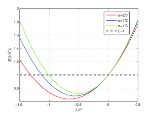
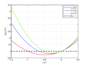
Fig. 1: The graph of $E(\lambda h^{\alpha})$ for 2-stage EFORK method (15) with $c_{2}^{\alpha}=\frac{2(\alpha!)^{2}}{(2\alpha)!}$ (left), and $c_{2}^{\alpha}=\frac{(\Gamma(2\alpha+1))^{2}}{\Gamma(3\alpha+1)\Gamma(\alpha+1)}$ (right).

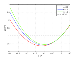
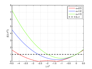
Fig. 2: The graph of $E(\lambda h^{\alpha})$ for 2-stage EFORK method (15) with $c_{2}^{\alpha}=\frac{4\Gamma(\alpha+1)}{\Gamma(3\alpha+1)}$(left), and $c_{2}^{\alpha}=\frac{\Gamma(\alpha+1)}{\Gamma(3\alpha+1)}$ (right).

Also, we apply the 3-stage EFORK method (21) to equation (41) and get

$$y_{n+1} =\left[1+\frac{\lambda h^{\alpha}}{\alpha!}+\frac{(\lambda h^{\alpha})^{2}}{(2\alpha)!}+\frac{(\lambda h^{\alpha})^{3}}{(3\alpha)!}\right]y_{n}\,.$$

Thus, the growth factor for 3-stage EFORK method (21) is

$$E(\lambda h^{\alpha})=1+\frac{\lambda h^{\alpha}}{\alpha!}+\frac{(\lambda h^{\alpha})^{2}}{(2\alpha)!}+\frac{(\lambda h^{\alpha})^{3}}{(3\alpha)!}\,.$$

The 3-stage EFORK method is absolutely stable if

$$|1+\frac{\lambda h^{\alpha}}{\alpha!}+\frac{(\lambda h^{\alpha})^{2}}{(2\alpha)!}+\frac{(\lambda h^{\alpha})^{3}}{(3\alpha)!}|\leqslant 1.$$

The graph of $E(\lambda h^{\alpha})$ for 3-stage EFORK method (21) is shown in Figure 3. In this Figure, we can see the interval of absolute stability for various $\alpha$.

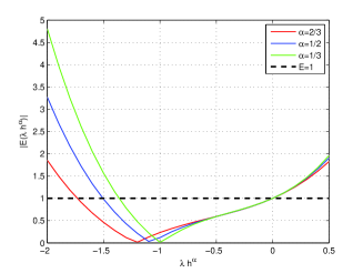
Fig. 3: The graph of $E(\lambda h^{\alpha})$ for 3-stage EFORK method (21).

Next, we apply the IFORK method (33) to equation (41) and get

$$E(\lambda h^{\alpha})=1+\frac{\frac{1}{\alpha!}\lambda h^{\alpha}}{1-\lambda h^{\alpha}\frac{\alpha!}{(2\alpha)!}},$$

with the interval of absolute stability $(-\infty,0)$, $\lambda<0$. In a similar manner, we can obtain the interval of absolute stability for IFORK method (34). As we can see, in implicit fractional RK methods, interval of absolute stability is very large and they are A stable.

6 Numerical examples

In order to demonstrate the effectiveness and order of accuracy of the proposed methods in sections 3-4, two examples are considered.



$\bf{Example}$ $\bf{1:}$ Let us consider fractional differential equation

$${}_{0}^{c}D_{t}^{\alpha}y(t)=-y(t)+\frac{t^{4-\alpha}}{\Gamma(5-\alpha)},\quad t\in[0,T],$$

$$y(0)=0,$$

where, the exact solution of the equation is $y(t)=t^{4}E_{\alpha,5}(-t^{\alpha})$.
For different values of $h$, $\alpha$ and $T$, the computed solutions are compared with the exact solution. We have reported the absolute error in time $T$ as:

$$E(h,T)=|y(t_{N^{m}})-y_{N^{m}}|.$$

Also, we calculated the computational orders of the presented method according to the following relation:

$$Log_{2}\frac{E(h,T)}{E(h/2,T)}.$$

The computed solutions by 2-stage EFORK method (15), 3-stage EFORK method (21) and IFORK methods (33) and (34) are reported in Tables 1-6. From the Tables 1-6, we can conclude that the computed orders of truncation errors is in a good agreement with the obtained results of sections 3-4 .

Table 1: 2-stage method (15) for $T=1$, $m=3$ in Example 1.

$\alpha$	$h$	$E(h,T)$	$Log_{2}\frac{E(h,T)}{E(h/2,T)}$
1/3	1/40	$1.09027e{-2}$	$1.1320$
	1/80	$4.97465e{-3}$	$1.0013$
	1/160	$2.48509e{-3}$	$0.9136$
	1/320	$1.31920e{-3}$	$0.8533$
	1/640	$7.30171e{-4}$	$*$

Table 2: 2-stage method (15) for $T=1$, $m=2$ in Example 1.

$\alpha$	$h$	$E(h,T)$	$Log_{2}\frac{E(h,T)}{E(h/2,T)}$
1/2	1/40	$2.05503e{-3}$	$1.2248$
	1/80	$8.79256e{-4}$	$1.1621$
	1/160	$3.92907e{-4}$	$1.1171$
	1/320	$1.81137e{-4}$	$1.0845$
	1/640	$8.54183e{-5}$	$*$

Table 3: 3-stage method (21) for $T=1$, $m=4$ in Example 1.

$\alpha$	$h$	$E(h,T)$	$Log_{2}\frac{E(h,T)}{E(h/2,T)}$
1/4	1/40	$9.94252e{-4}$	$0.8437$
	1/80	$5.54011e{-4}$	$0.8214$
	1/160	$3.13499e{-4}$	$0.8064$
	1/320	$1.79258e{-4}$	$0.7958$
	1/640	$1.03255e{-4}$	$*$

Table 4: 3-stage method (21) for $T=1$, $m=2$ in Example 1.

$\alpha$	$h$	$E(h,T)$	$Log_{2}\frac{E(h,T)}{E(h/2,T)}$
1/2	1/40	$7.45694e{-5}$	$1.5942$
	1/80	$2.46986e{-5}$	$1.5789$
	1/160	$8.26771e{-6}$	$1.5625$
	1/320	$2.79911e{-6}$	$1.5478$
	1/640	$9.57367e{-7}$	$*$

Table 5: IFORK methods for $T=1$, $m=2$ in Example 1.

$\alpha$	$h$	IFORK (33)	$Log_{2}\frac{E(h,T)}{E(h/2,T)}$	IFORK (34)	$Log_{2}\frac{E(h,T)}{E(h/2,T)}$
1/2	1/40	$1.86448e{-4}$	$1.0832$	$3.56080e{-4}$	$1.7307$
	1/80	$8.79978e{-5}$	$1.0492$	$1.07291e{-4}$	$1.6666$
	1/160	$4.25221e{-5}$	$1.0291$	$3.37953e{-5}$	$1.6191$
	1/320	$2.08361e{-5}$	$1.0174$	$1.10016e{-5}$	$1.5846$
	1/640	$1.02928e{-5}$	$*$	$3.66806e{-6}$	$*$

Table 6: IFORK methods for $T=1$, $m=3$ in Example 1.

$\alpha$	$h$	IFORK (33)	$Log_{2}\frac{E(h,T)}{E(h/2,T)}$	IFORK (34)	$Log_{2}\frac{E(h,T)}{E(h/2,T)}$
1/3	1/40	$3.04275e{-4}$	$0.9083$	$5.12337e{-3}$	$1.4661$
	1/80	$1.62123e{-4}$	$0.8746$	$1.85445e{-3}$	$1.3856$
	1/160	$8.84207e{-5}$	$0.8482$	$7.09751e{-4}$	$1.2940$
	1/320	$4.91160e{-5}$	$0.8255$	$2.89458e{-4}$	$1.2106$
	1/640	$2.77152e{-5}$	$*$	$1.25070e{-4}$	$*$

Fig 4, illustrates the error curves of the 2-stage EFORK method (15) and the 3-stage EFORK method (21) at $T=1,$ with $\alpha=1/2$, $m=2$ and different values of $N$.

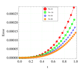
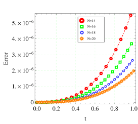
Fig. 4: The error curves of the 2-stage EFORK method (15) (left), and the error curves of the 3-stage EFORK method (21) (right) for Example 1.

$\bf{Example}$ $\bf{2:}$ Let us consider the following fractional differential equation from [6]:

$${}_{0}^{c}D_{t}^{\alpha}y(t)=\frac{2}{\Gamma(3-\alpha)}t^{2-\alpha}-\frac{1}{\Gamma(2-\alpha)}t^{1-\alpha}-y(t)+t^{2}-t,\quad t\in[0,T],$$

$$y(0)=0,$$

where the exact solution of the problem is $y(t)=t^{2}-t$.
For different values of $h$, $\alpha$ and $T$, the obtained results by 2-stage EFORK method (15), 3-stage EFORK method (21). IFORK methods (33) and (34) are shown in Tables 7-12.

Also, from the Tables 7-12, we can see that the computed orders is consistent with the given results of sections 3-4.

Fig 5, illustrates the numerical results of the 2-stage EFORK method (15) and the 3-stage EFORK method (21) at $T=1$ for $\alpha=1/2$, $m=2$ and different values of $N$. Also, Fig 6 illustrates the numerical results of the IFORK method (33) for Example 1 and Example 2 at $T=1$ for $\alpha=1/2$, $m=2$ and different values of $N$.

Table 7: 2-stage method (15) for $T=1$, $m=3$ in Example 2.

$\alpha$	$h$	$E(h,T)$	$Log_{2}\frac{E(h,T)}{E(h/2,T)}$
1/3	1/40	$1.00356e{-1}$	$1.1075$
	1/80	$4.65748e{-2}$	$0.9928$
	1/160	$2.34046e{-2}$	$0.9107$
	1/320	$1.24493e{-2}$	$0.8523$
	1/640	$6.89556e{-3}$	$*$

Table 8: 2-stage method (15) for $T=1$, $m=2$ in Example 2.

$\alpha$	$h$	$E(h,T)$	$Log_{2}\frac{E(h,T)}{E(h/2,T)}$
1/2	1/40	$1.77152e{-2}$	$1.2351$
	1/80	$7.52581e{-3}$	$1.1738$
	1/160	$3.33574e{-3}$	$1.1275$
	1/320	$1.52680e{-3}$	$1.0928$
	1/640	$7.15859e{-4}$	$*$

Table 9: 3-stage method (21) for $T=1$, $m=4$ in Example 2.

$\alpha$	$h$	$E(h,T)$	$Log_{2}\frac{E(h,T)}{E(h/2,T)}$
1/4	1/40	$9.90939e{-3}$	$0.8383$
	1/80	$5.54249e{-3}$	$0.8182$
	1/160	$3.14342e{-3}$	$0.8047$
	1/320	$1.79955e{-3}$	$0.7950$
	1/640	$1.03718e{-3}$	$*$

Table 10: 3-stage method (21) for $T=1$, $m=2$ in Example 2.

$\alpha$	$h$	$E(h,T)$	$Log_{2}\frac{E(h,T)}{E(h/2,T)}$
1/2	1/40	$5.79341e{-4}$	$1.5592$
	1/80	$1.96590e{-4}$	$1.5566$
	1/160	$6.68302e{-5}$	$1.5475$
	1/320	$2.28624e{-5}$	$1.5374$
	1/640	$7.87606e{-6}$	$*$

Table 11: IFORK methods for $T=1$, $m=2$ in Example 2.

$\alpha$	$h$	IFORK (33)	$Log_{2}\frac{E(h,T)}{E(h/2,T)}$	IFORK (34)	$Log_{2}\frac{E(h,T)}{E(h/2,T)}$
1/2	1/40	$1.52888e{-3}$	$1.0777$	$2.99223e{-3}$	$1.6608$
	1/80	$7.24362e{-4}$	$1.0464$	$9.46328e{-4}$	$1.6244$
	1/160	$3.50728e{-4}$	$1.0279$	$3.06932e{-4}$	$1.5943$
	1/320	$1.72002e{-4}$	$1.0171$	$1.01649e{-4}$	$1.5703$
	1/640	$8.49858e{-5}$	$*$	$3.42297e{-5}$	$*$

Table 12: IFORK methods for $T=1$, $m=3$ in Example 2.

$\alpha$	$h$	IFORK (33)	$Log_{2}\frac{E(h,T)}{E(h/2,T)}$	IFORK (34)	$Log_{2}\frac{E(h,T)}{E(h/2,T)}$
1/3	1/40	$2.84493e{-3}$	$0.9005$	$4.77620e{-2}$	$1.4860$
	1/80	$1.52403e{-3}$	$0.8707$	$1.70509e{-2}$	$1.3835$
	1/160	$8.33483e{-4}$	$0.8463$	$6.53520e{-3}$	$1.2859$
	1/320	$4.63592e{-4}$	$0.8246$	$2.68020e{-3}$	$1.2023$
	1/640	$2.61754e{-4}$	$*$	$1.16478e{-3}$	$*$

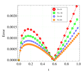
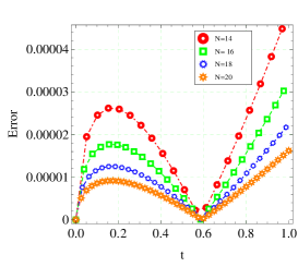
Fig. 5: The error curves of the 2-stage EFORK method (15) (left), and the 3-stage EFORK method (21) (right) in Example 2.

Table 13: $E(h,T)$ for $\alpha=1/2$, $m=2$ and different values of $T$.

$T$	2-stage-Exam.1	3-stage-Exam.1	2-stage-Exam.2	3-stage-Exam.2
0.5	$4.81351e{-6}$	$4.20218e{-8}$	$9.29068e{-5}$	$5.57177e{-7}$
1.0	$8.54183e{-5}$	$9.57367e{-7}$	$3.00335e{-3}$	$7.87606e{-6}$
1.5	$4.51426e{-4}$	$6.00243e{-6}$	$2.78127e{-3}$	$3.63915e{-5}$
2	$1.45778e{-3}$	$2.20455e{-5}$	$6.26033e{-3}$	$9.38735e{-5}$
3	$7.50603e{-3}$	$1.37070e{-4}$	$1.78449e{-2}$	$3.26003e{-4}$

Table 14: Optimal 2-stage method (15) for $T=1$, $m=2$.

$\alpha$	$h$	$E(h,T)$, Example 1	$E(h,T)$, Example 2
1/2	1/40	$7.35533e{-4}$	$6.12299e{-3}$
	1/80	$3.55401e{-4}$	$2.94885e{-3}$
	1/160	$1.72778e{-4}$	$1.43060e{-3}$
	1/320	$8.45336e{-5}$	$6.99024e{-4}$
	1/640	$4.15855e{-5}$	$3.43589e{-4}$

From these Tables, we conclude that the computational order for 2 and 3 stages EFORK methods are ${2\alpha}$ and ${3\alpha}$, respectively. As expected and seen in Tables and Figs, the 3-stage EFORK method in comparison with the 2-stage EFORK method, provides better results. In Table 13, the numerical results for different values of $T$ are shown.

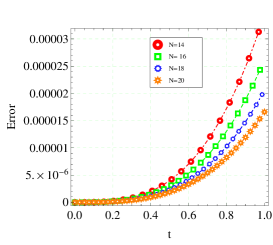
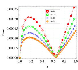
Fig. 6: The error curves of the IFORK method (33) in Example 1 (left), and Example 2 (right).

Also, the numerical results for optimal case $c_{2}^{\alpha}=\frac{(\Gamma(2\alpha+1))^{2}}{\Gamma(3\alpha+1)\Gamma(\alpha+1)}$, in 2-stage EFORK method are shown in Table 14 with $\alpha=1/2$ and different values of $h$.

7 Conclusions

This paper introduces new efficient FORK methods for FDEs based on Caputo generalized Taylor formulas. The proposed methods were examined for consistency, convergence, and stability. The interval of absolute stability of FORK methods has been determined, and implicit fractional order RK methods were shown to be A stable. Some examples were provided to demonstrate the effectiveness of these numerical schemes. We can obtain these results for Riemann–Liouville and Gronwald–Letnikov fractional derivatives accordingly.
Recently, a new concept of differentiation called fractal and fractional differentiation was suggested and numerically examined by many researchers [36, 37], where the differential operator has two orders: the first is fractional order and the second is the fractal dimension. These differential (integral) operators have not been studied intensively yet. In future work, we will extend the presented method for fractional differential equations with fractal–fractional derivatives.

References

- [1] Podlubny, I. Fractional Differential Equations; Academic Press: San Diego, CA, USA, 1999.
- [2] Hilfer, R. Applications of Fractional Calculus in Physics; World Scientific: Singapore, 2000.
- [3] Giona, M.; Roman, H.E. Fractional diffusion equation for transport phenomena in random media. Physica A 1992, 185, 87–97.
- [4] Diethelm, K. The Analysis of Fractional Differential Equations; Lecture Notes in Mathematics (LNM, Volume 2004); Springer: Berlin/Heidelberg, Germany, 2004.
- [5] Podlubny, I. Geometric and physical interpretation of fractional integration and fractional differentiation. Fract. Calc. Appl. Anal. 2002, 5, 367–386.
- [6] Odibat, Z.M.; Momani, S. An algorithm for the numerical solution of differential equations of fractional order. J. Appl. Math. Inform. 2008, 26, 15–27.
- [7] Gao, W.; Veeresha, P.; Prakasha, D.G.; Baskonus, H.M.; Ye, G. New numerical results for the Time-Fractional Phi-Four equation using a novel analytical approach. Symmetry 2020, 12, 478.
- [8] Postavaru, O.; Toma, A. Numerical solution of two-dimensional fractional-order partial differential equations using hybrid functions. Part. Diff. Eqs. Appl. Math. 2021, 4, 100099.
- [9] Aslan, E.; Kurkçu, O.K.; Sezer, M. A fast numerical method for fractional partial integro-differential equations with spatial-time delays. Appl. Numer. Math. 2021, 161, 525–539.
- [10] Garrappa, R. Numerical Solution of Fractional Differential Equations: A Survey and a Software. Mathematics 2018, 6, 16.
- [11] Sheng, C.; Cao, D.; Shen, J. Efficient spectral methods for PDEs with spectral fractional Laplacian. J. Sci. Comput. 2021, 88, 4.
- [12] Zhang, T.; Li, Y. Exponential Euler scheme of multi-delay Caputo–Fabrizio fractional-order differential equations. Appl. Math. Lett. 2021, 124, 107709.
- [13] Zhang, T.; Zhou, J.; Liao, Y. Exponentially stable periodic oscillation and Mittag–Leffler stabilization for fractional-order impulsive control neural networks with piecewise Caputo derivatives. IEEE Trans. Cyber. 2022, 52, 9670–9683.
- [14] Diethelm, K.; Walz, G. Numerical solution of fractional order differential equation by extrapolation. Numer. Algorithms 1997, 16, 231–253.
- [15] Diethelm, K.; Ford, N.J.; Freed, A.D. A Predictor-corrector approach for the numerical solution of fractional differential equations. Nonlinear Dynam. 2002, 29, 3–22.
- [16] Mokhtary, P.; Ghoreishi F. Convergence analysis of spectral Tau method for fractional Riccati differential equations.Bull. Iran. Math. Soc. 2014, 40, 1275–1290.
- [17] Langlands, T.; Henry, B. The accuracy and stability of an implicit solution method for the fractional diffusion equation. J. Comput. Phys. 2005, 205, 719–736.
- [18] Sun, Z.Z.; Wu, X. A fully discrete difference scheme for a diffusion-wave system. Appl. Numer. Math. 2006, 56, 193–209.
- [19] Gao, G.; Sun, Z.Z.; Zhang, H. A new fractional numerical differentiation formula to approximate the Caputo fractional derivative and its applications. J. Comput. Phys. 2014, 259, 33–50.
- [20] Cao, J.; Xu, C. A high order scheme for the numerical solution of the fractional ordinary differential equations. J. Comput. Phys. 2013, 238, 154–168.
- [21] Odibat, Z. Approximations of fractional integrals and Caputo fractional derivatives. Appl. Math. Comput. 2006, 178, 527–533.
- [22] Li, C.; Chen, A.; Ye, J. Numerical approaches to the fractional calculus and fractional ordinary differential equation. J. Comput. Phys. 2011, 230, 3352–3368.
- [23] Butcher, J.C. Numerical Methods for Ordinary Differential Equations; John Wiley & Sons: Chichester, UK, 2008.
- [24] Zingg, D.W.; Chisholm, T.T. Runge Kutta methods for linear ordinary differential equations. Appl. Numer. Math. 1999, 31, 227–238.
- [25] Houwen, P. The development of Runge-Kutta methods for partial differential equations. Appl. Numer. Math. 1996, 20, 261–272.
- [26] Butcher, J.C. Trees and numerical methods for ordinary differential equations. Numer. Algorithms 2010, 53, 153–170.
- [27] Butcher, J.C. Practical Runge Kutta methods for scientific computation. ANZIAM. J. 2009, 50, 333–342.
- [28] Lubich, C. Runge-Kutta theory for Volterra and Abel integral equations of the second kind. Math. Comput. 1983, 41, 87–102.
- [29] Brunner, H.; Hairer, E.; Norsett, S.P. Runge-Kutta theory for Volterra integral equations of the second kind. Math. Comput. 1982, 39, 147–163.
- [30] Izzo, G.; Russo, E.; Chiapparelli, C. Highly stable Runge–Kutta methods for Volterra integral equations. Appl. Numer. Math. 2012, 62, 1002–1013.
- [31] Ostermann, A.; Roche, M. Runge-Kutta Methods for Partial Differential Equations and Fractional Orders of Convergence. Math. Comp. 1992, 59, 403–420.
- [32] Ostermann, A.; Roche, M. Rosenbrock methods for partial differential equations and fractional orders of convergence. SIAM J. Numer. Anal. 1993, 30, 1084–1098.
- [33] Srivastava, H.M. Operators of Fractional Calculus and Their Applications. Mathematics 2019, 6, 157.
- [34] Odibat, Z.; Shawagfeh, N. Generalized Taylor’s formula. Appl. Math. Comput. 2007, 186, 286–293.
- [35] Jain, M.K. Numerical Solution of Differential Equations, 2nd ed.; Wiley Eastern Limited: Bridgewater, NJ, USA, 1991.
- [36] Youssri, Y.H.; Atta, A.G. Spectral Collocation Approach via Normalized Shifted Jacobi Polynomials for the Nonlinear Lane-Emden Equation with Fractal-Fractional Derivative, Fractal Fract. 2023, 7, 133.
- [37] Youssri, Y.H. Orthonormal ultraspherical operational matrix algorithm for fractal–fractional Riccati equation with generalized Caputo derivative. Fractal Fract. 2021, 5, 100.