Poisson multi-Bernoulli mixture filter with general target-generated measurements and arbitrary clutter

Abstract

This paper shows that the Poisson multi-Bernoulli mixture (PMBM) density is a multi-target conjugate prior for general target-generated measurement distributions and arbitrary clutter distributions. That is, for this multi-target measurement model and the standard multi-target dynamic model with Poisson birth model, the predicted and filtering densities are PMBMs. We derive the corresponding PMBM filtering recursion. Based on this result, we implement a PMBM filter for point-target measurement models and negative binomial clutter density in which data association hypotheses with high weights are chosen via Gibbs sampling. We also implement an extended target PMBM filter with clutter that is the union of Poisson-distributed clutter and a finite number of independent clutter sources. Simulation results show the benefits of the proposed filters to deal with non-standard clutter.

I Introduction

Multi-target filtering consists of estimating the current states of an unknown and variable number of targets based on noisy sensor measurements up to the current time step. It is a key component of numerous applications, for example, defense [1], automotive systems [2] and air traffic control [3]. Multi-target filtering is usually addressed using probabilistic modelling, with the main approaches being multiple hypothesis tracking [4], joint probabilistic data association [5] and random finite sets [6].

In detection-based multi-target filtering, sensors collect scans of data that may contain target-generated measurements as well as clutter, which refers to undesired detections. For example, in radar, clutter can be caused by reflections from the environment, such as terrain, sea and rain, or other undesired objects [7, 8]. Multi-target filters applied to real data must then account for these clutter measurements for suitable performance, for instance, sea clutter and land clutter in radar data [9], false detections in image data [10, 11], false detections in audio visual data [12], and underwater clutter in active sonar data [13, 14].

In the standard detection model, clutter is modelled as a Poisson point process (PPP) [6]. The PPP is motivated by the fact that, for sufficiently high sensor resolution and independent clutter reflections in each sensor cell, the detection process can be accurately approximated as a PPP [15]. The PPP is also convenient mathematically and it can be characterised by its intensity function on the single-measurement space.

For the point-target measurement model, PPP clutter and the standard multi-target dynamic model with PPP birth, the posterior is a Poisson multi-Bernoulli mixture (PMBM) [16, 17]. The PMBM consists of the union of a PPP, representing undetected targets, and an independent multi-Bernoulli mixture (MBM) representing targets that have been detected at some point and their data association hypotheses. The posterior density is also a PMBM for the extended target model [18] and for a general target-generated measurement model [19], both with PPP clutter and the standard dynamic model. Extended target modelling is required when, due to the sensor resolution and the target extent, a target may generate more than one detection at each time step [20]. This makes the data association problem considerably more challenging than for point targets. The general target generated-measurement model includes the point and extended target cases as particular cases, and can for example be used when there can be simultaneous point and extended targets in a scenario [19].

If the birth model is multi-Bernoulli instead of PPP, the posterior density in the above cases is an MBM, which is obtained by setting the Poisson intensity of the PMBM filter to zero and by adding the Bernoulli components of the birth process in the prediction step. The MBM filter can also be written in terms of Bernoulli components with deterministic target existence, which results in the MBM₀₁ filter [17, Sec. IV]. It is also possible to add unique labels to the target states in the MBM and MBM₀₁ filters. The (labelled) MBM₀₁ filtering recursions are analogous to the $\delta$-generalised labelled multi-Bernoulli ($\delta$-GLMB) filtering recursions [21, 22].

All the above recursions to compute the posterior assume PPP clutter, but other clutter distributions are also important in various contexts, for instance, to model bursts of radar sea clutter [23]. For general target-generated measurements and arbitrary clutter density, the Bernoulli filter was proposed in [24], and the probabilistic hypothesis density (PHD) filter, which provides a PPP approximation to the posterior, was derived in [25]. The corresponding PHD filter update depends on the set derivative of the logarithm of the probability generating functional (PGFL) of the clutter process. A version of this PHD filter update, written in terms of densities, which is more suitable for implementation than [25], is provided in [26]. There are also other PHD filter variants with non-PPP clutter for point targets, for example, a PHD filter with negative binomial clutter [27], a second order PHD filter with Panjer clutter [28], and a linear-complexity cumulant-based filter for clutter described by its intensity and second-order cumulant [29, 30]. A cardinalised PHD filter with general target-generated measurements and arbitrary clutter is derived in [31]. Another approach is to estimate the states of Bernoulli clutter generators by including them in the multi-target state [6, 32].

This paper shows that for general target-generated measurements and arbitrary clutter density, the posterior is also a PMBM and we derive the filtering recursion. This contribution extends the family of closed-form recursions to calculate the posterior to a more general detection-based measurement model. As a direct result, this paper also derives the corresponding (labelled or not) MBM and MBM₀₁ filters, including $\delta$-GLMB filters. We also directly obtain the Poisson multi-Bernoulli (PMB) filter, which can be derived by Kullback-Leibler divergence minimisation on a target space augmented with auxiliary variables [16, 33]. We also propose a Gibbs sampling algorithm for selecting global hypotheses with high weights [34, 35, 21, 36] for the PMBM filter for point targets and clutter that is an independent and an identically distributed (IID) cluster process [6] with arbitrary cardinality distribution. We show via simulation results the advantages of the proposed filter in two scenarios: one scenario for point targets and IID clutter with negative binomial cardinality distribution, and another scenario for extended targets where there are a finite number of clutter sources.

The rest of this paper is organised as follows. Section II introduces the models and an overview of the PMBM posterior. The PMBM filter update is presented in Section III. The Gibbs sampling data association algorithm for point-target PMBM filtering with arbitrary clutter is proposed in Section IV. Finally, simulation results and conclusions are provided in Sections V and VI.

II Models and overview of the PMBM posterior

This section presents the dynamic and measurement models in Section II-A, and an overview of the PMBM posterior in Section II-B, with its global hypotheses in Section II-C.

II-A Models

A target state is denoted by $x$ and it contains the variables that describe its current dynamics, such as position and velocity, and maybe other attributes, such as orientation and extent. The state $x\in\mathcal{X}$, where $\mathcal{X}$ is a locally compact, Hausdorff and second-countable (LCHS) space [6]. The set of targets at time $k$ is $X_{k}\in\mathcal{F}\left(\mathcal{X}\right)$, where $\mathcal{F}\left(\mathcal{X}\right)$ represents the set of finite subsets of $\mathcal{X}$.

Targets move according to the standard multi-target dynamic model [6]. Given $X_{k}$, each target $x\in X_{k}$ survives with probability $p^{S}\left(x\right)$ and moves with a transition density $g\left(\cdot\left|x\right.\right)$, or disappears with probability $1-p^{S}\left(x\right)$. New targets are born at time step $k$ according to an independent Poisson point process (PPP) with intensity $\lambda_{k}^{B}\left(\cdot\right)$.

A measurement state $z\in\mathcal{Z}$ contains a sensor measurement. The set $Z_{k}\in\mathcal{F}\left(\mathcal{Z}\right)$ of measurements at time $k$ is the union of target-generated measurements and independent clutter measurements, modelled by

• Each target $x\in X_{k}$ generates a set of measurements with density $f\left(\cdot|x\right)$.

• The set of clutter measurements at each time step has density $c\left(\cdot\right)$.

• Given $X_{k}$, the measurements generated by different targets are independent of each other and of the clutter measurements.

It should be noted that $f\left(\cdot|x\right)$ is a general density for target-generated measurements and we can accommodate any probabilistic model for target-generated measurements. The probability that at least one measurement is generated from the target (effective probability of detection [37]) is $1-f\left(\emptyset|x\right)$. For example, the standard point target model in which a target $x$ is detected with probability $p^{D}\left(x\right)$ and generates a measurement with density $l(\cdot|x)$ [6], is obtained by

$$f\left(Z|x\right) =\begin{cases}1-p^{D}\left(x\right)&Z=\emptyset\\ p^{D}\left(x\right)l(z|x)&Z=\left\{z\right\}\\ 0&\left|Z\right|>1.\end{cases}$$ (1)

In the standard extended target model, we can receive more than one measurement from a target. Specifically, a target $x$ is detected with probability $p^{D}\left(x\right)$ and, if detected, it generates a PPP measurement with intensity $\gamma\left(x\right)l(\cdot|x)$, where $l(\cdot|x)$ is a single-measurement density and $\gamma\left(x\right)$ is the expected number of measurements [20, 38]. It is obtained by

$$f\left(Z|x\right) =\begin{cases}1-p^{D}\left(x\right)+p^{D}\left(x\right)e^{-\gamma\left(x\right)}&Z=\emptyset\\ p^{D}\left(x\right)\gamma^{\left|Z\right|}\left(x\right)e^{-\gamma\left(x\right)}\prod_{z\in Z}l(z|x)&\left|Z\right|>0.\end{cases}$$ (2)

We can also combine both (1) and (2) to model coexisting point and extended targets, or use any of the probabilistic extended target models in [20]. In addition, the choice of $f\left(\cdot|x\right)$ can also take into account reflectivity models and the propagation conditions in the environment [8, 39, 40, 41].

II-B PMBM posterior

We will show in this paper that, for the dynamic and measurement models in Section II-A, the predicted and posterior densities are PMBMs. That is, given the sequence of measurements $\left(Z_{1},...,Z_{k^{\prime}}\right)$, the density $f_{k|k^{\prime}}\left(\cdot\right)$ of $X_{k}$ with $k^{\prime}\in\left\{k-1,k\right\}$ is

$$f_{k|k^{\prime}}\left(X_{k}\right) =\sum_{Y\uplus W=X_{k}}f_{k|k^{\prime}}^{\mathrm{p}}\left(Y\right)f_{k|k^{\prime}}^{\mathrm{mbm}}\left(W\right),$$ (3)

$$f_{k|k^{\prime}}^{\mathrm{p}}\left(X_{k}\right) =e^{-\int\lambda_{k|k^{\prime}}\left(x\right)dx}\prod_{x\in X_{k}}\lambda_{k|k^{\prime}}\left(x\right),$$ (4)

$$f_{k|k^{\prime}}^{\mathrm{mbm}}\left(X_{k}\right) =\sum_{a\in\mathcal{A}_{k|k^{\prime}}}w_{k|k^{\prime}}^{a}\sum_{\uplus_{l=1}^{n_{k|k^{\prime}}}X^{l}=X_{k}}\prod_{i=1}^{n_{k|k^{\prime}}}f_{k|k^{\prime}}^{i,a^{i}}\left(X^{i}\right),$$ (5)

where $\lambda_{k|k^{\prime}}\left(\cdot\right)$ is the intensity of the PPP $f_{k|k^{\prime}}^{\mathrm{p}}\left(\cdot\right)$, representing undetected targets, and $f_{k|k^{\prime}}^{\mathrm{mbm}}\left(\cdot\right)$ is a multi-Bernoulli mixture representing targets that have been detected at some point up to time step $k^{\prime}$. The sum in (3) is the convolution sum, which implies that the PPP and MBM are independent [6]. The symbol $\uplus$ denotes the disjoint union and the sum is taken over all mutually disjoint (and possibly empty) sets $Y$ and $W$ whose union is $X_{k}$.

The MBM in (5) has $n_{k|k^{\prime}}$ Bernoulli components (potential targets), each with $h_{k|k^{\prime}}^{i}$ local hypotheses. There is a local hypothesis $a^{i}\in\left\{1,...,h_{k|k^{\prime}}^{i}\right\}$ for each Bernoulli $i>0$. To handle arbitrary clutter, we also introduce a local hypothesis $a^{0}\in\left\{1,...,h_{k|k^{\prime}}^{0}\right\}$ for clutter. Each $a^{i}$ is an index that associates the $i$-th Bernoulli, for $i\geq 0$, or the clutter, for $i=0$, to a specific sequence of subsets of the measurement set, see Section II-C. A global hypothesis is denoted by $a=\left(a^{0},a^{1},...,a^{n_{k|k^{\prime}}}\right)\in\mathcal{A}_{k|k^{\prime}}$, where $\mathcal{A}_{k|k^{\prime}}$ is the set of global hypotheses, see Section II-C. The weight of global hypothesis $a$ is $w_{k|k^{\prime}}^{a}$ and meets

$$w_{k|k^{\prime}}^{a}\propto\prod_{i=0}^{n_{k|k^{\prime}}}w_{k|k^{\prime}}^{i,a^{i}}$$ (6)

where $w_{k|k^{\prime}}^{i,a^{i}}$ is the weight of the $i$-th Bernoulli component, or clutter if $i=0$, with local hypothesis $a^{i}$, and $\sum_{a\in\mathcal{A}_{k|k^{\prime}}}w_{k|k^{\prime}}^{a}=1$. A difference with PMBM filters with PPP clutter [16, 18, 19] is that global hypotheses and weights explicitly consider clutter, with index $i=0$.

The $i$-th Bernoulli component with local hypothesis $a^{i}$ has a density

$$f_{k|k^{\prime}}^{i,a^{i}}\left(X\right) =\begin{cases}1-r_{k|k^{\prime}}^{i,a^{i}}&X=\emptyset\\ r_{k|k^{\prime}}^{i,a^{i}}p_{k|k^{\prime}}^{i,a^{i}}\left(x\right)&X=\left\{x\right\}\\ 0&\mathrm{otherwise}\end{cases}$$ (7)

where $r_{k|k^{\prime}}^{i,a^{i}}$ is the probability of existence and $p_{k|k^{\prime}}^{i,a^{i}}\left(\cdot\right)$ is the single-target density. It should be noted that in this paper we use the following nomenclature for Bernoulli components, densities and local hypotheses: Each Bernoulli component, which is indexed by $i$ and is initiated by a non-empty subset of measurements at a given time step (see Section III), has $h_{k|k^{\prime}}^{i}$ local hypotheses, each with an associated Bernoulli density, indexed by $i,a^{i}$. Then, the total number of Bernoulli densities in (5) across all global hypotheses is $\sum_{i=1}^{n_{k|k^{\prime}}}h_{k|k^{\prime}}^{i}$, and the number of multi-Bernoulli densities is $|\mathcal{A}_{k|k^{\prime}}|$, which denotes the cardinality of $\mathcal{A}_{k|k^{\prime}}$.

II-C Set of global hypotheses

We proceed to describe the set $\mathcal{A}_{k|k^{\prime}}$ of global hypotheses. We denote the measurement set at time step $k$ as $Z_{k}=\left\{z_{k}^{1},...,z_{k}^{m_{k}}\right\}$. We refer to measurement $z_{k}^{j}$ using the pair $\left(k,j\right)$ and the set of all such measurement pairs up to and including time step $k$ is denoted by $\mathcal{M}_{k}$. Then, a local hypothesis $a^{i}$ for $i=\left\{0,1,...,n_{k|k^{\prime}}\right\}$ has an associated set of measurement pairs denoted as $\mathcal{M}_{k}^{i,a^{i}}\subseteq\mathcal{M}_{k}$. The set $\mathcal{A}_{k|k^{\prime}}$ of all global hypotheses meets

$$\mathcal{A}_{k|k^{\prime}}= \left\{\left(a^{0},a^{1},...,a^{n_{k|k^{\prime}}}\right):a^{i}\in\left\{1,...,h_{k|k^{\prime}}^{i}\right\}\,\forall i,\right.$$

$$\left.\bigcup_{i=0}^{n_{k|k^{\prime}}}\mathcal{M}_{k^{\prime}}^{i,a^{i}}=\mathcal{M}_{k^{\prime}},\mathcal{M}_{k^{\prime}}^{i,a^{i}}\cap\mathcal{M}_{k^{\prime}}^{j,a^{j}}=\emptyset,\,\forall i\neq j\right\}.$$

That is, each measurement must be assigned to a local hypothesis, and there cannot be more than one local hypothesis with the same measurement. In this paper, we construct the (trees of) local hypotheses recursively, and we allow for more than one measurement to be associated to the same local hypothesis at the same time step, i.e., $\mathcal{M}_{k}^{i,a^{i}}$ may contain zero, one or more measurements. At time step zero, the filter is initiated with $n_{0|0}=0$, $w_{0|0}^{0,1}=1$, $h_{0|0}^{0}=1$, and $\mathcal{M}_{0}^{0,1}=\emptyset$.

III General PMBM filter

This section presents the PMBM filter for general target-generated measurements and arbitrary clutter, with models described in Section II-A. We consider the standard dynamic model so the prediction step is the standard PMBM prediction step [16, 17]. The update is presented in Section III-A. We provide a discussion and extension of the result to other filter variants in Sections III-B and III-C. The PMBM for point targets and arbitrary clutter is explained in Section III-D. Finally, an analysis of the number of global hypotheses for different PMBM filters is provided in Section III-E.

III-A General PMBM update

Given two real-valued functions $a\left(\cdot\right)$ and $b\left(\cdot\right)$ on the target space, we denote their inner product as

$$\left\langle a,b\right\rangle =\int a\left(x\right)b\left(x\right)dx.$$ (8)

Then, the update of the predicted PMBM $f_{k|k-1}\left(\cdot\right)$ with $Z_{k}$ is given in the following theorem.

Theorem 1.

Assume the predicted density $f_{k|k-1}\left(\cdot\right)$ is a PMBM of the form (3). Then, the updated density $f_{k|k}\left(\cdot\right)$ with set $Z_{k}=\left\{z_{k}^{1},...,z_{k}^{m_{k}}\right\}$ is a PMBM with the following parameters. The number of Bernoulli components is $n_{k|k}=n_{k|k-1}+2^{m_{k}}-1$. The intensity of the PPP is

$$\lambda_{k|k}\left(x\right) =f\left(\emptyset|x\right)\lambda_{k|k-1}\left(x\right).$$ (9)

Let $Z_{k}^{1},...,Z_{k}^{2^{m_{k}}-1}$ be the non-empty subsets of $Z_{k}$. The updated number of local clutter hypotheses is $h_{k|k}^{0}=2^{m_{k}}h_{k|k-1}^{0}$ such that a new local clutter hypothesis is included for each previous local clutter hypothesis and either a misdetection or an update with a non-empty subset of $Z_{k}$. The updated local clutter hypotheses with no clutter at time step $k$, $a^{0}\in\left\{1,...,h_{k|k-1}^{0}\right\}$, have parameters $\mathcal{M}_{k}^{0,a^{0}}=\mathcal{M}_{k-1}^{0,a^{0}}$,

$$w_{k|k}^{0,a^{0}} =w_{k|k-1}^{0,a^{0}}c\left(\emptyset\right).$$ (10)

For a previous local clutter hypothesis $\widetilde{a}^{0}\in\left\{1,...,h_{k|k-1}^{0}\right\}$ in the predicted density, the new local clutter hypothesis generated by a set $Z_{k}^{j}$ has $a^{0}=\widetilde{a}^{0}+h_{k|k-1}^{0}j$,

$$\mathcal{M}_{k}^{0,a^{0}} =\mathcal{M}_{k-1}^{0,\widetilde{a}^{0}}\cup\left\{\left(k,p\right):z_{k}^{p}\in Z_{k}^{j}\right\},$$ (11)

$$w_{k|k}^{0,a^{0}} =w_{k|k-1}^{0,a^{0}}c\left(Z_{k}^{j}\right).$$ (12)

For Bernoulli components continuing from previous time steps $i\in\left\{1,...,n_{k|k-1}\right\}$, a new local hypothesis is included for each previous local hypothesis and either a misdetection or an update with a non-empty subset of $Z_{k}$. The updated number of local hypotheses is $h_{k|k}^{i}=2^{m_{k}}h_{k|k-1}^{i}$. For missed detection hypotheses, $i\in\left\{1,...,n_{k|k-1}\right\}$, $a^{i}\in\left\{1,...,h_{k|k-1}^{i}\right\}$:

$$\mathcal{M}_{k}^{i,a^{i}} =\mathcal{M}_{k-1}^{i,a^{i}},$$ (13)

$$l_{k|k}^{i,a^{i},\emptyset} =\big{\langle}p_{k|k-1}^{i,a^{i}},f\left(\emptyset|\cdot\right)\big{\rangle},$$ (14)

$$w_{k|k}^{i,a^{i}} =w_{k|k-1}^{i,a^{i}}\left[1-r_{k|k-1}^{i,a^{i}}+r_{k|k-1}^{i,a^{i}}l_{k|k}^{i,a^{i},\emptyset}\right],$$ (15)

$$r_{k|k}^{i,a^{i}} =\frac{r_{k|k-1}^{i,a^{i}}l_{k|k}^{i,a^{i},\emptyset}}{1-r_{k|k-1}^{i,a^{i}}+r_{k|k-1}^{i,a^{i}}l_{k|k}^{i,a^{i},\emptyset}},$$ (16)

$$p_{k|k}^{i,a^{i}}(x) =\frac{f\left(\emptyset|x\right)p_{k|k-1}^{i,a^{i}}(x)}{l_{k|k}^{i,a^{i},\emptyset}}.$$ (17)

For a Bernoulli component $i\in\left\{1,...,n_{k|k-1}\right\}$ with a local hypothesis $\widetilde{a}^{i}\in\left\{1,...,h_{k|k-1}^{i}\right\}$ in the predicted density, the new local hypothesis generated by a set $Z_{k}^{j}$ has $a^{i}=\widetilde{a}^{i}+h_{k|k-1}^{i}j$, $r_{k|k}^{i,a^{i}}=1$, and

$$\mathcal{M}_{k}^{i,a^{i}} =\mathcal{M}_{k-1}^{i,\widetilde{a}^{i}}\cup\left\{\left(k,p\right):z_{k}^{p}\in Z_{k}^{j}\right\},$$ (18)

$$l_{k|k}^{i,a^{i},Z_{k}^{j}} =\bigg{\langle}p_{k|k-1}^{i,\widetilde{a}^{i}},f\left(Z_{k}^{j}|\cdot\right)\bigg{\rangle},$$ (19)

$$w_{k|k}^{i,a^{i}} =w_{k|k-1}^{i,\widetilde{a}^{i}}r_{k|k-1}^{i,\widetilde{a}^{i}}l_{k|k}^{i,a^{i},Z_{k}^{j}},$$ (20)

$$p_{k|k}^{i,a^{i}}(x) =\frac{f\left(Z_{k}^{j}|x\right)p_{k|k-1}^{i,\widetilde{a}^{i}}(x)}{l_{k|k}^{i,a^{i},Z_{k}^{j}}}.$$ (21)

For the new Bernoulli component initiated by subset $Z_{k}^{j}$, whose index is $i=n_{k|k-1}+j$, we have two local hypotheses ($h_{k|k}^{i}=2$), one corresponding to a non-existent Bernoulli density

$$\mathcal{M}_{k}^{i,1}=\emptyset,\;w_{k|k}^{i,1}=1,\;r_{k|k}^{i,1}=0,$$ (22)

and the other with $r_{k|k}^{i,2}=1$, $w_{k|k}^{i,2}=l_{k|k}^{Z_{k}^{j}}$ and

$$\mathcal{M}_{k}^{i,2} =\left\{\left(k,p\right):z_{k}^{p}\in Z_{k}^{j}\right\},$$ (23)

$$l_{k|k}^{Z_{k}^{j}} =\bigg{\langle}\lambda_{k|k-1},f\left(Z_{k}^{j}|\cdot\right)\bigg{\rangle},$$ (24)

$$p_{k|k}^{i,2}(x) =\frac{f\left(Z_{k}^{j}|x\right)\lambda_{k|k-1}(x)}{l_{k|k}^{Z_{k}^{j}}}.\quad\square$$ (25)

Theorem 1 is proved in Appendix A.

We can see that the updated PPP intensity in (9) is the predicted intensity multiplied by the probability of receiving no measurements, as in the PMBM filters for PPP clutter [16, 17, 18, 19]. Contrary to PMBM filters with PPP clutter, the general PMBM filter extends local and global hypotheses to explicitly consider clutter data associations, whose weights depend on the clutter density via (12). As data associations for clutter are separated from the target hypotheses, the probability of existence of new Bernoulli components $r_{k|k}^{i,2}$ is equal to one, as in the PMBM filter for unknown clutter rate in [42]. This is different from the PMBM filters for PPP clutter, where, for each separate measurement, the hypotheses for clutter and the first detection of a new target are merged into one. After merging, the probability of existence of a new Bernoulli component depends on the clutter intensity, and the number of global hypotheses for PPP clutter is lower, see Section II-C.

We also observe that each non-empty subset of $Z_{k}$ generates a new Bernoulli, which has two local hypotheses. It is also possible to instead reformulate the update to only generate $m_{k}$ new Bernoulli components by increasing the number of local hypotheses of the new Bernoulli components [43, Sec. IV]. We proceed to illustrate the differences between the hypotheses generated by this PMBM update, and the update with PPP clutter with an example.

Example 2.

Let us consider that the predicted density is a PPP and the measurement set at time step 1 is $Z_{1}=\left\{z_{1}^{1},z_{1}^{2}\right\}$. The non-empty subsets are $Z_{1}^{1}=\left\{z_{1}^{1}\right\}$, $Z_{1}^{2}=\left\{z_{1}^{2}\right\}$ and $Z_{1}^{3}=\left\{z_{1}^{1},z_{1}^{2}\right\}$. For general target-generated measurements (including extended targets) with PPP clutter, we create 3 Bernoulli components, each initiated by $Z_{1}^{1}$, $Z_{1}^{2}$ and $Z_{1}^{3}$, with two local hypotheses [18, 19]. Therefore we have $\mathcal{M}_{1}^{1,2}=\left\{\left(1,1\right)\right\}$, $\mathcal{M}_{1}^{2,2}=\left\{\left(1,2\right)\right\}$, $\mathcal{M}_{1}^{3,2}=\left\{\left(1,1\right),\left(1,2\right)\right\}$. The number of global hypotheses is the number of partitions of $Z_{1}$, which is 2.

For general target-generated measurements and arbitrary clutter, Theorem 1 also creates 3 Bernoulli components, each initiated by $Z_{1}^{1}$, $Z_{1}^{2}$ and $Z_{1}^{3}$, with two local hypotheses. The difference now is that $\emptyset$, $Z_{1}^{1}$, $Z_{1}^{2}$ and $Z_{1}^{3}$ can also be associated to clutter, and each of these subsets generates a local hypothesis for clutter, which has then 4 local hypotheses. That is, $\mathcal{M}_{1}^{0,1}=\emptyset$, $\mathcal{M}_{1}^{0,2}=\left\{\left(1,1\right)\right\}$, $\mathcal{M}_{1}^{0,3}=\left\{\left(1,2\right)\right\}$, and $\mathcal{M}_{1}^{0,4}=\left\{\left(1,1\right),\left(1,2\right)\right\}$. The number of global hypotheses is 5. $\diamondsuit$

III-B Discussion

In this subsection, we discuss the spooky action at a distance that may appear when we deal with arbitrary clutter, and an alternative choice of hypotheses when the clutter density has some additional structure.

III-B1 Spooky action at a distance

If there is one measurement far from all previous targets represented in the PMBM, the PMBM filters with PPP clutter generate a Bernoulli component that appears in all global hypotheses and whose probability of existence does not depend on the other measurements that have been received in far away areas. That is, the probability of existence of a newly detected isolated target only depends on the local situation.

For arbitrary clutter PMBM filters, the new Bernoulli component has probability of existence one in some, but not all, global hypotheses. The weights of these global hypotheses depend on the clutter density evaluated for all measurements. Therefore, the probability of existence of the new target (considering all global hypotheses) can depend on all measurements, even if they are far away, a phenomenon usually referred to as spooky action at a distance [44]. This effect is illustrated the following example.

Example 3.

Let us consider the update of a PPP, which results in a PMB density, with two measurements $\{z_{1}^{k},z_{2}^{k}\}$ that are far away from each other. Then, a single target cannot generate both measurements, and the probability of this event is zero. If clutter is PPP, the probability of existence of a Bernoulli component generated by $z_{1}^{k}$ is [19]

$$r_{k|k} =\frac{l_{k|k}^{\left\{z_{1}^{k}\right\}}}{\lambda^{C}\left(z_{1}^{k}\right)+l_{k|k}^{\left\{z_{1}^{k}\right\}}}$$ (26)

where $l_{k|k}^{\left\{z_{1}^{k}\right\}}$ is given by (24) and $\lambda^{C}\left(\cdot\right)$ is the clutter intensity. The probability of existence $r_{k|k}$ is independent of $z_{2}^{k}$.

If clutter is arbitrary, there are four global hypotheses with non-negligible weights, representing the events that $z_{1}^{k}$ and $z_{2}^{k}$ correspond to either a newly detected target or clutter. The probability of existence, considering all global hypotheses, of the target initiated by measurement $z_{1}^{k}$ is

$$r_{k|k} =\frac{l_{k|k}^{\left\{z_{1}^{k}\right\}}\left(c\left(\left\{z_{2}^{k}\right\}\right)+l_{k|k}^{\left\{z_{2}^{k}\right\}}c\left(\emptyset\right)\right)}{w},$$ (27)

$$w =l_{k|k}^{\left\{z_{1}^{k}\right\}}\left(c\left(\left\{z_{2}^{k}\right\}\right)+l_{k|k}^{\left\{z_{2}^{k}\right\}}c\left(\emptyset\right)\right)$$

$$\quad+c\left(\left\{z_{1}^{k}\right\}\right)l_{k|k}^{\left\{z_{2}^{k}\right\}}+c\left(\left\{z_{1}^{k},z_{2}^{k}\right\}\right).$$ (28)

If $c\left(\cdot\right)$ is a PPP, then, (27) simplifies to (26), and the probability of existence is independent of $z_{2}^{k}$. However, in general, $r_{k|k}$ depends on $z_{2}^{k}$, which implies that a far-away measurement influences the probability of existence of a newly detected target in another area, resulting in a spooky action at a distance phenomenon. $\diamondsuit$

It should also be noted that it is possible to design $c\left(\cdot\right)$ to avoid spooky action by setting it as the union of different, independent sources of clutter in non-overlapping areas.

III-B2 Alternative choice of hypotheses

Theorem 1 proves that the update of a PMBM density with general target-generated measurements and arbitrary clutter is a PMBM and provides an expression of the update. Nevertheless, if the clutter has additional structure, for example, it is a PMB, i.e., clutter being the union of a conventional PPP clutter plus $n_{c}$ Bernoulli sources of clutter, it is possible to design an alternative hypothesis structure with $n_{c}$ sources of clutter and integrate the PPP clutter into the probability of existence of new Bernoulli components. Therefore, the clutter structure can be exploited to design PMBM filters tailored to specific clutter models. An example of the PMBM update with clutter that is the union of PPP clutter and a finite number of independent clutter sources is provided in Appendix B.

III-C Extension to MBM, MBM₀₁, PMB, and labelled filters

Theorem 1 also holds for a predicted density of the form MBM or MBM₀₁ by setting $\lambda_{k|k-1}\left(\cdot\right)=0$. Therefore, we obtain the MBM filter by applying the standard MBM prediction step [17, Sec. III.E], which includes multi-Bernoulli birth model, followed by Theorem 1 update. The MBM₀₁ filter is the same as the MBM filter with the difference that the MBM₀₁ filter prediction step expands each Bernoulli density into two hypotheses with deterministic target existence [17, Eq. (36)]. This results in an unnecessary exponential increase in the number of global hypotheses in the prediction step, so it is not recommended.

It is also relevant to notice that the general PMBM update in Theorem 1 also includes Bernoulli densities with deterministic existence (when updating an existing Bernoulli density with a non-empty measurement set or initiating a new Bernoulli component). Nevertheless, these Bernoulli densities with deterministic existence are required to deal with arbitrary clutter. In contrast, the MBM₀₁ filter creates the deterministic Bernoulli densities in the prediction, which is not necessary.

Both MBM and MBM₀₁ can be directly extended to include deterministic, fixed labels assigned to each Bernoulli density of the birth model without changing the filtering recursion [17, Sec. IV.V]. This procedure yields the labelled MBM and labelled MBM₀₁ filters. The $\delta$-GLMB filtering recursion is analogous to the labelled MBM₀₁ filtering recursion, so this procedure provides the $\delta$-GLMB filter for general target-generated measurements and arbitrary clutter.

PMB (and multi-Bernoulli) filters for arbitrary clutter can be obtained by projecting the updated PMBM into a PMB using KLD minimisation [16, 33, 45, 43].

III-D PMBM filter for point targets and arbitrary clutter

The equations in Theorem 1 are also valid for point targets with arbitrary clutter. In this setting, the target-generated measurement density is given by (1). With the definitions of local and global hypotheses in Section II-C, many hypotheses associate more than one measurement to the same Bernoulli component at the same time. However, according to (1), the weights of these hypotheses will be zero. Therefore, we can directly exclude these hypotheses from the set $\mathcal{A}_{k|k}$ of global hypotheses, by restricting the cardinality of $\mathcal{M}_{k}^{i,a^{i}}$ to zero or one for $i>0$. This approach, combined with the corresponding prediction step, provides the PMBM, MBM, MBM₀₁ ($\delta$-GLMB) filtering recursions for point targets and arbitrary clutter.

III-E Number of global hypotheses

In this section, we calculate the number of global hypotheses of PMBM filters to compare: 1) PPP clutter versus arbitrary clutter, and 2) point targets versus the general target-generated measurement model. This analysis helps us understand the differences in the hypothesis structures of the PMBM filters and provides a measure of the complexity of the corresponding data association problems. To simplify the analysis, we first consider the update of a PPP prior in Section III-E1, and then the update of a PMB prior in Section III-E2.

III-E1 Update of a PPP prior

We calculate the number of global hypotheses when we update a PPP prior. In the PMBM filter for point targets and PPP clutter, the number of global hypotheses after updating a PPP prior is 1. With a general target-generated measurement model and PPP clutter, the number of global hypotheses is the number of partitions of the measurement set, which is the Bell number $B_{m_{k}}$ [6, App. D].

In the PMBM filter with point-target measurement model and arbitrary clutter, the number of global hypotheses is $2^{m_{k}}$, representing the events that each measurement is either a newly detected target or clutter. With general target-generated measurements and arbitrary clutter, the number of global hypotheses is

$$\sum_{c=0}^{m_{k}}\left(\begin{array}[]{c}m_{k}\\ c\end{array}\right)B_{m_{k}-c}$$ (31)

which is equal to $B_{m_{k}+1}$ applying [6, Eq. (D.4)]. That is, in (31), we go through all possible numbers $c$ of clutter measurements. Then, the binomial coefficient indicates the number of subsets with $c$ clutter measurements and $B_{m_{k}-c}$ indicates the number of partitions of the rest of the measurements, each generating a new global hypothesis.

III-E2 Update of a Poisson multi-Bernoulli

We calculate the number of global hypotheses generated in the update of the $j$-th global hypothesis of a prior PMBM, which represents a PMB. To calculate the total number of global hypotheses, we sum these results for all global hypotheses. The number of Bernoulli components in the PMB with existence probability higher than zero is denoted by $n^{j}$.

For point targets and PPP clutter, the number of global hypotheses is

$$N_{p,p}\left(n^{j},m_{k}\right) =\sum_{p=0}^{\min\left(n^{j},m_{k}\right)}p!\left(\begin{array}[]{c}m_{k}\\ p\end{array}\right)\left(\begin{array}[]{c}n^{j}\\ p\end{array}\right).$$ (36)

That is, we go through all possible numbers $p$ of detected targets among the ones that are represented by the Bernoulli components, the number of ways of selecting $p$ measurements and $p$ targets, and the number of permutations of $p$ elements (ways to associate $p$ measurements to $p$ targets). It can also be noticed that $m_{k}-p$ is the number of detections that are associated to either clutter or newly detected targets.

For general target-generated measurements and PPP clutter, the number of global hypotheses is [36, Sec. V]

$$N_{g,p}\left(n^{j},m_{k}\right) =\sum_{l=0}^{m_{k}}\left\{\begin{array}[]{c}m_{k}\\ l\end{array}\right\}N_{p,p}\left(n^{j},l\right)$$ (39)

where the factor in the brackets is the Stirling number of the second kind, which indicates the number of ways of partitioning a set with $m_{k}$ elements into $l$ non-empty cells. Starting the sum in (39) with $l=0$ enables us to count one partition when $m_{k}=0$.

For point targets and arbitrary clutter, the number of global hypotheses is

$$N_{p,a}\left(n^{j},m_{k}\right) =\sum_{c=0}^{m_{k}}\left(\begin{array}[]{c}m_{k}\\ c\end{array}\right)N_{p,p}\left(n^{j},m_{k}-c\right).$$ (42)

That is, we first go through all possible clutter hypotheses with $c$ clutter measurements. The remaining $m_{k}-c$ measurements can be assigned either to previously detected targets or to new targets, with at most one measurement per target.

For general target-generated measurements and arbitrary clutter, the number of global hypotheses is

$$N_{g,a}\left(n^{j},m_{k}\right) =\sum_{c=0}^{m_{k}}\left(\begin{array}[]{c}m_{k}\\ c\end{array}\right)N_{g,p}\left(n^{j},m_{k}-c\right).$$ (45)

That is, we first go through all possible clutter hypotheses with $c$ clutter measurements. The remaining $m_{k}-c$ measurements are assigned either to clutter or to new targets, following (39).

We show the number of global hypotheses of the filters after updating a PMB prior for different number of measurements in Table I, where the case $n^{j}=0$ corresponds to a PPP prior. It can be observed that considering general target-generated and arbitrary clutter significantly increases the number of global hypotheses compared to point targets and PPP clutter.

Table I: Number of PMBM global hypotheses after updating a PMB prior with $n^{j}$ targets and $m_{k}$ measurements

Target		Point						General
Clutter		PPP			Arbitrary			PPP			Arbitrary
$n^{j}$		0	1	4	0	1	4	0	1	4	0	1	4
$m_{k}$	1	1	2	5	2	3	6	1	2	5	2	3	6
	2	1	3	21	4	8	32	2	5	26	5	10	37
	3	1	4	73	8	20	152	5	15	141	15	37	235
	4	1	5	209	16	48	648	15	52	799	52	151	1540
	5	1	6	501	32	112	2,512	52	203	4,736	203	674	10,427
	10	1	11	8,501	1,024	6,144	850,944	115,975	678,570	67,310,847	678,570	3,535,027	247,126,450

IV Data associations in point-target PMBM filter with arbitrary clutter via Gibbs sampling

In this section, we develop a tractable PMBM filter for point targets and arbitrary clutter. A key challenge in this context is to handle the intractable growth in the number of data association hypotheses. For PPP clutter, we can use Murty’s algorithm to select the $K$-best updated global hypotheses generated from a single predicted global hypothesis, representing a PMB [46, 17], and then prune the other hypotheses. However, for arbitrary clutter, the data association problem is no longer an assignment problem [47] and thus we cannot use Murty’s algorithm. In this section, we explain how to use Gibbs sampling to select $K$-good updated global hypotheses from a predicted global hypothesis [34, 35, 21, 36]. That is, Gibbs sampling does not necessarily find the $K$-best global hypotheses, but it samples global hypotheses according to their weights, which implies that global hypotheses with higher weights are more likely to be selected.

IV-A Notation

To simplify notation in this section, we drop time indices in the number of measurements $m$ and the measurement set $\left\{z^{1},...,z^{m}\right\}$. In addition, the Bernoulli densities for the predicted global hypothesis, representing a PMB, have parameters $\left(r^{i},p^{i}(\cdot)\right)$ for $i\in\left\{1,...,n_{k|k-1}\right\}$.

Then, we recall that for the point target model, after the update, we have $n_{k|k}=n_{k|k-1}+m$ Bernoulli components, which includes $n_{k|k-1}$ predicted Bernoulli components and the new $m$ Bernoulli components, one generated by each measurement. The data associations can be represented as a vector $\gamma_{1:m}=\left(\gamma_{1},...,\gamma_{m}\right)$ where $\gamma_{j}\in\{0,1,...,n_{k|k}\}$ is the Bernoulli component index associated to the $j$-th measurement and $\gamma_{i}\neq\gamma_{j}$ for all $i\neq j$ such that $\gamma_{i}>0$ and $\gamma_{j}>0$. If $\gamma_{j}=0$, it means that the $j$-th measurement is clutter. The set of vectors $\gamma_{1:m}$ that meet this property is denoted by $\Gamma$.

We also use $1_{\Gamma}\left(\cdot\right)$ to denote the indicator function of set $\Gamma$: $1_{\Gamma}\left(\gamma_{1:m}\right)=1$ if $\gamma_{1:m}\in\Gamma$, and $1_{\Gamma}\left(\gamma_{1:m}\right)=0$ otherwise.

IV-B Arbitrary clutter density

The probability of data association $\gamma_{1:m}$, without accounting for the weight of the predicted global hypothesis, is

$$p\left(\gamma_{1:m}\right) \propto 1_{\Gamma}\left(\gamma_{1:m}\right)c\left(Z_{c}\left(\gamma_{1:m}\right)\right)\prod_{j=1:\gamma_{j}>0}^{m}\eta^{j}\left(\gamma_{j}\right)$$ (46)

where the measurement set corresponding to clutter is

$$Z_{c}\left(\gamma_{1:m}\right) =\left\{z^{j}:\gamma_{j}=0\right\}$$ (47)

and

$$\eta^{j}\left(\gamma_{j}\right)$$

$$\;=\begin{cases}\frac{r^{\gamma_{j}}\int p^{D}\left(x\right)l\left(z^{j}|x\right)p^{\gamma_{j}}(x)dx}{1-r^{\gamma_{j}}\left\langle p^{\gamma_{j}},p^{D}\right\rangle}&\gamma_{j}\leq n_{k|k-1}\\ \int p^{D}\left(x\right)l\left(z^{j}|x\right)\lambda_{k|k-1}\left(x\right)dx&n_{k|k-1}<\gamma_{j}\leq n_{k|k}.\end{cases}$$ (48)

In (48), the second line corresponds to the weight of new Bernoulli components, see (24). The first line corresponds to the weight of the predicted Bernoulli components with a detection $z^{j}$, see (20), divided by the misdetection weight, see (15), both using the point target measurement model (1).

To obtain samples from density (46) using Gibbs sampling, we calculate the conditional density [48]

$$p\left(\gamma_{q}|\gamma_{1:q-1},\gamma_{q+1:m}\right) \propto p\left(\gamma_{1:m}\right)$$ (49)

$$\propto 1_{\Gamma}\left(\gamma_{1:m}\right)c\left(Z_{c}\left(\gamma_{1:m}\right)\right)$$

$$\quad\times\prod_{j=1:\gamma_{j}>0}^{m}\eta^{j}\left(\gamma_{j}\right)$$ (50)

where $q\in\{1,...,m\}$. As $\gamma_{1:q-1},\gamma_{q+1:m}$ are constants in (50), $l^{j}\left(\gamma_{j}\right)$ for $j\neq q$ are constants too, and we can write

$$p\left(\gamma_{q}|\gamma_{1:q-1},\gamma_{q+1:m}\right)$$

$$\propto\begin{cases}1_{\Gamma}\left(\gamma_{1:m}\right)c\left(Z_{c}\left(\gamma_{1:m}\right)\right)\eta^{q}\left(\gamma_{q}\right)&\gamma_{q}>0\\ c\left(Z_{c}\left(\gamma_{1:m}\right)\right)&\gamma_{q}=0\end{cases}$$ (51)

where we have used that $\left(\gamma_{1:q-1},0,\gamma_{q+1:m}\right)\in\Gamma$. Equation (51) can be evaluated for all possible values $\gamma_{q}\in\{0,1,...,m\}$, and therefore, we can sample from this categorical distribution. To perform Gibbs sampling, we can start with $\gamma_{1:m}$ having all entries equal to zero, and sample $\gamma_{q}$ from $q=1$ to $m$ for a total number of $K$ times. Then, as in [21], we remove the repeated samples of data association hypotheses to yield the newly generated data association hypotheses. In the implementations, we set $K=\left\lceil N_{h}\cdot w_{j}\right\rceil$, where $N_{h}$ is the maximum number of global hypotheses.

IV-C Uniform IID cluster clutter

In this subsection, we specify (51) for the case where the clutter $c\left(\cdot\right)$ follows an IID cluster process [6] whose the single-measurement density $\breve{c}\left(\cdot\right)$ is uniform in the field-of view $A$. That is,

$$c\left(Z\right) =|Z|!\rho_{c}\left(|Z|\right)\prod_{z\in Z}\breve{c}\left(z\right)$$ (52)

$$\breve{c}\left(z\right) =u_{A}\left(z\right)$$ (53)

where $\rho_{c}\left(|Z|\right)$ is the cardinality distribution and $u_{A}\left(\cdot\right)$ is a uniform density in $A$.

Let $m_{c}$ denote the number of clutter measurements in $\gamma_{1:q-1},\gamma_{q+1:m}$, i.e.,

$$m_{c} =\sum_{j=1:j\neq q}^{m}\delta_{0}\left[\gamma_{j}\right]$$ (54)

where $\delta_{j}[\cdot]$ is the Kronecker delta at $j$. Then, considering that all measurements are in the field-of-view, (51) becomes

$$p\left(\gamma_{q}|\gamma_{1:q},\gamma_{q+1:m}\right)$$

$$\propto\begin{cases}1_{\Gamma}\left(\gamma_{1:m}\right)\eta^{q}\left(\gamma_{q}\right)\rho_{c}\left(m_{c}\right)m_{c}!\frac{1}{|A|^{m_{c}}}&\gamma_{q}>0\\ \rho_{c}\left(m_{c}+1\right)\left(m_{c}+1\right)!\frac{1}{|A|^{m_{c}+1}}&\gamma_{q}=0\end{cases}$$ (55)

where $|A|$ is the area (or the hypervolume) of $A$.

V Simulation experiments

In this section, we evaluate the developed PMBM and PMB filters in two scenarios. The main objective of these simulations is to study how filters deal with non-standard sources of clutter. Section V-A presents a scenario with point targets and IID cluster clutter with a negative binomial cardinality distribution. Section V-B presents a scenario with extended targets and a number of independent clutter sources of clutter.

V-A Point targets and negative binomial IID cluster clutter

In this section, we consider point targets with clutter being an IID cluster process with negative binomial (NB) cardinality distribution [49]. We compare the following filters: the standard PMBM and PMB filter (with PPP clutter assumption), and the arbitrary clutter PMBM and PMB filters, referred to as A-PMBM and A-PMB. The rest of the parameters are [17]: maximum number of global hypotheses $N_{h}=5,000$, threshold for MBM pruning $10^{-4}$, threshold for pruning the PPP weights $\Gamma_{p}=10^{-5}$, threshold for pruning Bernoulli densities $\Gamma_{b}=10^{-5}$, and ellipsoidal gating with threshold 20. These filters use Estimator 3 as it provides the best performance among the standard PMBM estimators [17, Sec. VI] in this scenario. Estimator 3 obtains the global hypothesis with a deterministic cardinality with highest weight and then reports the mean of the targets in this hypothesis.

Additionally, we have implemented two filters with multi-Bernoulli birth and PPP clutter: the MBM filter [17, 50], and the $\delta$-GLMB filter with joint prediction and update [21]. The $\delta$-GLMB filter has been implemented with 7,000 global hypotheses and pruning threshold $10^{-15}$. All the previous filters have been implemented using Gibbs sampling to select relevant global hypotheses in the update of each predicted global hypothesis. We have also implemented a Gaussian mixture PHD filter for PPP clutter [6, 51] and a Gaussian mixture PHD filter for NB IID clutter in [27], which we refer to as the NB-PHD filter. The PHD filters have parameters: pruning threshold $10^{-5}$, merging threshold 0.1, and maximum number of Gaussian components 30.

V-A1 Clutter density

We consider an IID cluster clutter density with uniform single-measurement density in the field of view, as in (52) and (53). Its cardinality distribution is NB, $\rho_{c}\left(m\right)=\mathrm{NB}\left(m;r,p\right)$, with $r>0$, $p\in\left[0,1\right]$, and [49]

$$\mathrm{NB}\left(m;r,p\right) =\frac{\Gamma\left(r+m\right)}{\Gamma\left(r\right)\Gamma\left(m+1\right)}p^{r}\left(1-p\right)^{m}$$ (56)

where $\Gamma\left(\cdot\right)$ is the gamma function. Its mean and variance are

$$\mathrm{E}\left[m\right]=\frac{\left(1-p\right)r}{p},\>\mathrm{V}\left[m\right]=\frac{\left(1-p\right)r}{p^{2}}.$$ (57)

Therefore, if we denote $\mathrm{E}\left[m\right]=\overline{\lambda}^{C}$ and $\mathrm{V}\left[m\right]=a^{C}\overline{\lambda}^{C}$ with $a^{C}>1$, using (56), we can obtain parameters $r$ and $p$ based on $\overline{\lambda}^{C}$ and $a^{C}$

$$r=\frac{\overline{\lambda}^{C}}{a^{C}-1},\;p=\frac{1}{a^{C}}.$$ (58)

Parameter $a^{C}$ indicates the over-dispersion w.r.t. the Poisson distribution. In fact, the NB distribution results from integrating out the rate of a Poisson distribution, with the rate having a gamma distribution [49], so it is always over-dispersed. This means that for NB distribution its variance is always larger than its mean, making it suitable for scenarios with high clutter variance. For $a^{C}\rightarrow 1$, the NB distribution tends to a Poisson distribution with parameter $\overline{\lambda}^{C}$.

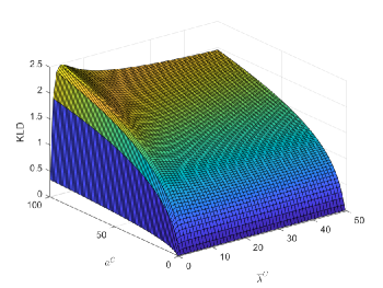
Figure 1: KLD $\mathrm{D}\left(\mathrm{P}||\mathrm{NB}\right)$ between Poisson and negative binomial distributions for different values of $\overline{\lambda}^{C}$ and $a^{C}$. As $a^{C}$ increases, the distributions become more different.

The KLD $\mathrm{D}\left(\mathrm{P}||\mathrm{NB}\right)$ between the Poisson (P) and NB distributions with the same mean $\overline{\lambda}^{C}$ w.r.t. different values of $\overline{\lambda}^{C}$ and $a^{C}$ is shown in Figure 1. We can see that, for $a^{C}\rightarrow 1$ and $\overline{\lambda}^{C}\rightarrow 0$, the distributions tend to be more similar, and they differ as these parameters increase, mainly due to increments in $a^{C}$. This is important as it implies that if the $\mathrm{NB}$ distribution is quite similar to the Poisson, then, the PMBM filter with PPP clutter is expected to outperform the PMBM filter with arbitrary clutter due to its improved hypothesis structure, as pointed out in Section III-E.

V-A2 Simulation results

The target state is $x=[p_{x},v_{x},p_{y},v_{y}]^{\top}$, which contains its position and velocity. The dynamic model is a nearly-constant velocity model [52]

$$g\left(x_{k}|x_{k-1}\right) =\mathcal{N}\left(x_{k};Fx_{k-1},Q\right)$$

$$F=I_{2}\otimes\begin{bmatrix}1&T\\ 0&1\end{bmatrix},\,Q=qI_{2}\otimes\begin{bmatrix}T^{3}/3&T^{2}/2\\ T^{2}/2&T\end{bmatrix},$$

where $\otimes$ is the Kronecker product, $q=0.01\,\mathrm{m}^{2}/\mathrm{s}^{3}$, the sampling time $T=1\,\mathrm{s}$, and $\mathcal{N}\left(x;\overline{x},P\right)$ represents a Gaussian density with mean $\overline{x}$ and covariance matrix $P$ evaluated at $x$. The probability of survival is $p^{S}=0.99$. The birth process is a PPP with a Gaussian intensity

$$\lambda_{k}^{B}\left(x\right) =w_{k}^{b}\mathcal{N}\left(x;\overline{x}_{k}^{b},P_{k}^{b}\right),$$ (59)

where $\overline{x}_{k}^{b}=\left[150\,(\mathrm{m}),0\,(\mathrm{m/s}),150\,(\mathrm{m}),0\,(\mathrm{m/s})\right]^{\top}$, $P_{k}^{b}=\mathrm{diag}\left(\left[50^{2}\,(\mathrm{m}^{2}),1\,(\mathrm{m}^{2}/\mathrm{s}^{2}),50^{2}\,(\mathrm{m}^{2}),1\,(\mathrm{m}^{2}/\mathrm{s}^{2})\right]\right)$ and the weight $w_{1}^{b}=5$ for $k=1$, and $w_{k}^{b}=0.1$ for $k>1$. The weight $w_{k}^{b}$ represents the expected number of new born targets at time step $k$ [6].

The ground truth set of trajectories, shown in Figure 2, is generated by sampling the above dynamic model for 81 time steps. The target starting at time step 1 at around $[150,210]\,(\mathrm{m}),$ and the one starting at time step 50 at around $[95,95]\,(\mathrm{m})$ get in close proximity at around time step 52.

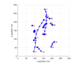
Figure 2: Ground truth set of trajectories for the point target scenario. Initial trajectory positions are marked with filled circles and their positions every ten time steps are marked with a circle. The black numbers next to birth positions indicate the time of birth and the red numbers the last time a target is alive.

The filters with multi-Bernoulli birth (MBM and $\delta$-GLMB) use 9 Bernoulli birth components at time step 1 with probability of existence 5/9, mean $\overline{x}_{k}^{b}$ and covariance matrix $P_{k}^{b}$. This choice approximately covers the support of the cardinality of the PPP, and sets the same PHD for the multi-Bernoulli and PPP birth models [6]. For $k>1$, these filters use a Bernoulli birth with probability of existence $w_{k}^{b}$, mean $\overline{x}_{k}^{b}$ and covariance matrix $P_{k}^{b}$.

At each time step, the sensor measures positions with likelihood

$$l\left(z|x\right) =\mathcal{N}\left(z;Hx,R\right)$$

$$H=I_{2}\otimes\begin{bmatrix}1&0\end{bmatrix},\,R=4I_{2}\,(\mathrm{m}^{2}),$$

and a probability of detection $p^{D}=0.9$. Clutter is uniformly distributed in the region of interest $A=[0,300]\times[0,300]\,(\mathrm{m}\times\mathrm{m})$ such that $\breve{c}\left(z\right)=u_{A}\left(z\right)$. The NB clutter parameters are $a^{C}=20$ and $\overline{\lambda}^{C}=10$.

We evaluate the performances of the filters using Monte Carlo simulation with 100 runs. We obtain the root mean square generalised optimal subpattern assignment (RMS-GOSPA) metric error ($p=2$, $c=10\,\mathrm{m}$, $\alpha=2$) for the position elements at each time step [53]. The resulting GOSPA errors as well as their decomposition into localisation error for properly detected targets, and costs for missed and false targets are shown in Figure 3. The peaks in Figure 3 correspond to the time steps in which targets are born or die, see Figure 2. These peaks arise as it usually takes at least 2 time steps to estimate a new born target and also to stop reporting it when it dies. These peaks happen for all filters, though they are more difficult to spot on the PHD filters as they have a higher number of missed and false targets throughout all time steps. A-PMBM and A-PMB filters are the filters with best performance, closely followed by PMBM and PMB filters. The $\delta$-GLMB filter provides higher errors, specially due to missed targets. The MBM filter performs worse, and the PHD filters have the worst performance, as they provide a less accurate approximation to the posterior.

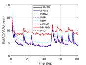
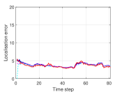
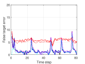
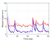
Figure 3: RMS GOSPA errors ($\mathrm{m)}$ and their decomposition against time for the point target scenario.

The computational times in seconds to run one Monte Carlo simulation on an Intel core i5 laptop are: 43.4 (A-PMBM), 40.7 (A-PMB), 20.2 (PMBM), 14.7 (PMB), 20.8 (MBM), 45.6 ($\delta$-GLMB), 1.1 (NB-PHD) and 1.1 (PHD). The PHD filters are the fastest algorithms, with the lowest performance. This is to be expected as they propagate a PPP through the filtering recursion so the structure of the posterior and the data association problem is simplified at the cost of lower performance. The A-PMBM and A-PMB filters have a higher computational burden than PMBM and PMB filters due to the higher number of global hypotheses and the extra calculations with negative binomial clutter. The $\delta$-GLMB filter has a higher computational burden due to its global hypothesis structure and implementation parameters [17].

Table II: RMS-GOSPA errors ($\mathrm{m)}$ across time for different $p^{D}$

$p^{D}$	0.95	0.9	0.8	0.7
A-PMBM	5.18	5.53	6.17	6.85
A-PMB	5.12	5.50	6.16	6.82
PMBM	5.25	5.65	6.34	7.06
PMB	5.26	5.67	6.38	7.10
MBM	7.16	7.18	7.50	8.07
$\delta$-GLMB	5.74	6.10	6.74	7.60
NB-PHD	6.86	9.31	11.56	13.28
PHD	7.12	9.28	12.04	13.72

The RMS-GOSPA errors considering all time steps in the simulation for several values of $p^{D}$ are shown in Table II. We can see that the filter with lowest error for all $p^{D}$ is the A-PMB filter tightly followed by the A-PMBM filter. While A-PMBM is the theoretical optimal filter, for a fixed number of global hypotheses and a sub-optimal estimator, A-PMB can outperform A-PMBM, especially in scenarios without challenging multi-target crossings. In particular, at each A-PMBM update, new Bernoulli components have probability of existence either 0 or 1, which requires a high number of global hypotheses (see Section III-E) that are updated separately at subsequent time steps. On the other hand, the A-PMB filter projects all the 0-1 hypotheses from the same Bernoulli component into a single Bernoulli density, providing a compact representation. As expected, the higher the probability of detection, the lower the error for all filters.

Table III: RMS-GOSPA errors ($\mathrm{m)}$ across time for different NB clutter parameters

$a^{C}$	2				10				20				40
$\overline{\lambda}^{C}$	1	5	10	15	1	5	10	15	1	5	10	15	1	5	10	15
A-PMBM	5.15	5.45	5.71	5.98	5.05	5.35	5.63	5.84	5.04	5.29	5.53	5.76	4.93	5.21	5.42	5.60
A-PMB	5.14	5.45	5.65	5.86	5.05	5.34	5.59	5.76	5.04	5.28	5.50	5.69	4.95	5.20	5.39	5.56
PMBM	5.13	5.45	5.65	5.86	5.11	5.41	5.66	5.88	5.14	5.40	5.65	5.88	5.13	5.40	5.62	5.83
PMB	5.14	5.46	5.67	5.88	5.12	5.41	5.69	5.90	5.15	5.43	5.67	5.91	5.14	5.42	5.64	5.86
MBM	5.27	6.23	6.32	6.40	5.22	6.61	6.82	6.85	5.27	6.91	7.12	7.18	5.26	7.09	7.38	7.61
$\delta$-GLMB	5.36	5.73	5.99	6.24	5.40	5.79	6.03	6.28	5.43	5.84	6.10	6.31	5.42	5.85	6.08	6.32
NB-PHD	9.13	9.22	9.42	9.73	8.90	9.22	9.29	9.54	8.87	9,08	9.31	9.48	8.86	8.99	9.24	9.34
PHD	9.13	9.20	9.44	9.80	9.09	9.12	9.28	9.76	9.07	9.07	9.28	9.67	9.12	8.97	9.16	9.50

We now proceed to analyse the performances of the filters for different clutter parameters. The RMS-GOSPA errors considering all time steps in the simulation for several values of $a^{C}$ and $\overline{\lambda}^{C}$ ($p^{D}=0.9$) are shown in Table III. The A-PMB filter is most of the times the best performing filter closely followed by the A-PMBM filter. The standard PMB and PMBM filters tend to work better in comparison with A-PMBM and A-PMB filters for low value of $a^{C}$. This is expected as, for values of $a^{C}$ close to 1, the negative binomial and Poisson distributions become alike, see Figure 1, and it becomes beneficial to use the standard filters with PPP clutter due to the improved hypothesis representation, see Section III-E. In fact, for $a^{C}=2$, the PMBM filter is the best performing filter overall. The $\delta$-GLMB filter has higher errors than the previous filters, and is followed by the MBM filter. PHD filters are the filters with the worst performance.

V-B Extended targets with independent clutter sources

In this section, we consider a scenario with extended targets where the clutter is the union of independent PPP and a number of stationary extended sources, see Appendix B. We compare the following filters with their gamma Gaussian inverse-Wishart (GGIW) implementations: the standard extended target PMBM and PMB filter (with PPP clutter assumption) [18, 43], the extended target PMBM and PMB filters with arbitrary clutter, also referred to as A-PMBM and A-PMB. We also compare with the GGIW implementations of the MBM filter [43] and the $\delta$-GLMB filter [22].

All PMBM-PMB filters have been implemented using a two-step clustering and assignment approach to select relevant global hypotheses in the update of each previous global hypotheses [20]. Specifically, we first apply the density-based spatial clustering of applications with noise (DB-SCAN) [54] using 25 different distance values equally spaced between 0.1 and 5 to obtain a set of different measurement partitions, and then for each measurement partition and global hypothesis $a$, we apply Murty’s algorithm [46] to find the $\lceil 20w_{k|k}^{a}\rceil$ best cluster-to-Bernoulli assignments. The rest of the parameters are: maximum number of global hypotheses $N_{h}=20$, threshold for MBM pruning $10^{-2}$, threshold for pruning the PPP weights $\Gamma_{p}=10^{-3}$, threshold for pruning Bernoulli densities $\Gamma_{b}=10^{-3}$, estimator 1 with threshold 0.4, and ellipsoidal gating with threshold 20. The $\delta$-GLMB filter has been implemented as in [22] with a maximum number of global hypotheses $N_{h}=20$.

The target state in GGIW implementation is $x=(\gamma,\xi,X)$, where $\gamma$ represents the expected number of measurements per target, $\xi=[p_{x},v_{x},p_{y},v_{y}]^{\top}$ contains the target current position and velocity, and $X$ is a positive definite matrix with size 2, describing the target ellipsoidal shape. The dynamical model for the kinematic state $\xi$ is the same as the one used for point target tracking, and states $\gamma$ and $X$ remain unchanged over time. The probability of survival $p^{S}=0.99$.

The birth process is a PPP with a GGIW intensity with weight $w_{k}^{b}=0.1$ for all time steps. Its GGIW density consists of a gamma distribution with mean 5 and shape 100, a Gaussian distribution with mean $\bar{x}_{k}^{b}=[150\,(\mathrm{m)},0\,(\mathrm{m/s)},150\,(\mathrm{m)},0\,(\mathrm{m/s)}]^{\top}$ and covariance matrix $P_{k}^{b}=\text{diag}([50^{2}\,(\mathrm{m}^{2}),1\,(\mathrm{m}^{2}/\mathrm{s}^{2}),50^{2}\,(\mathrm{m}^{2}),1\,(\mathrm{m}^{2}/\mathrm{s}^{2})])$, and an inverse-Wishart distribution with mean $\text{diag}([4,4])$ $(\mathrm{m}^{2})$ and degrees of freedom 100. The ground truth set of trajectories, shown in Figure 4, is generated by sampling the above dynamic model for 81 time steps. The MBM and $\delta$-GLMB use a Bernoulli birth with probability of existence 0.1 and the same mean and covariance matrix so that their PHDs match.

At each time step, a target is detected with probability $p^{D}=0.9$, and, if it is detected, the target measurements are a PPP with Poisson rate $5$ and single measurement density $\mathcal{N}(z;H\xi,sX+R)$ where scaling factor $s=1/4$ and measurement noise covariance $R=\text{diag}([1/4,1/4])$ $\,(\mathrm{m}^{2})$. There are four independent stationary clutter sources, located at $[100,100]^{\top}$, $[100,200]^{\top}$, $[200,100]^{\top}$ and $[200,200]^{\top}$ $\,(\mathrm{m)}$, respectively. Each stationary clutter source is detected with probability $0.98$, and, if it is detected, its measurements are a PPP with Poisson rate $10$ and Gaussian measurement density with covariance $\text{diag}([2,2])\,(\mathrm{m}^{2})$. The additional PPP clutter is uniformly distributed in the region of interest $A=[0,300]\times[0,300]\,(\mathrm{m}\times\mathrm{m})$ with Poisson clutter rate $\bar{\lambda}^{C}=20$.

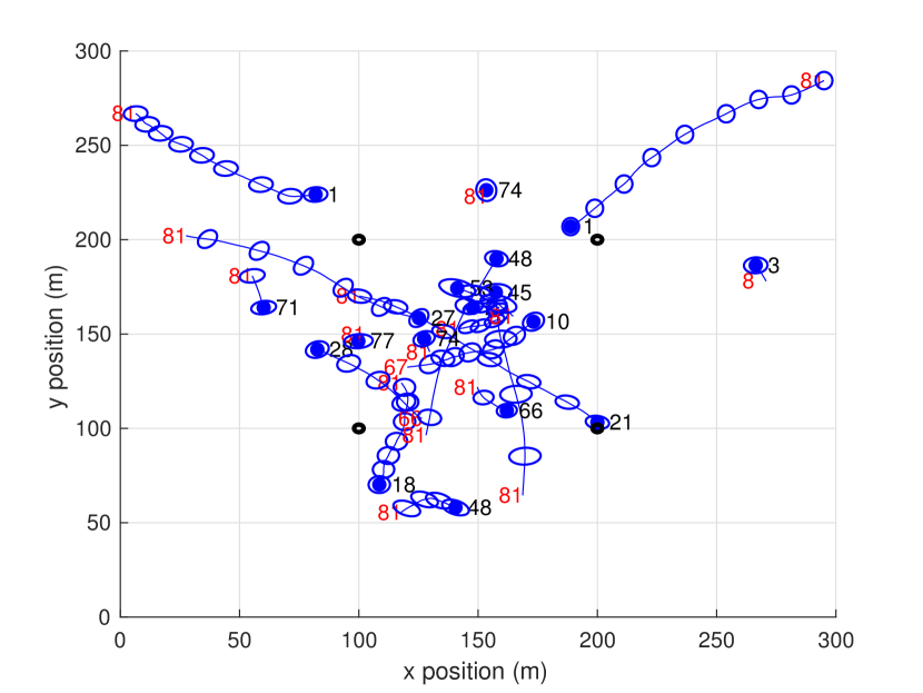
Figure 4: Ground truth set of trajectories for the extended target scenario. Initial trajectory positions are marked with filled circles and their extents (in blue ellipses) are shown every ten times. The four stationary sources are marked with black circles. The black numbers next to birth positions indicate the time of birth and the red numbers the last time a target is alive. At time step 21, a target is born adjacent to the stationary source at $[200,100]^{\top}\,(\mathrm{m})$. At time step 48, there is a target born nearby an existing target.

We evaluate the performances of the filters using Monte Carlo simulation with 100 runs. We obtain the root mean square GOSPA metric error ($p=2$, $c=10\,\mathrm{m}$, $\alpha=2$) at each time step, where the base measure is given by the Gaussian Wasserstein distance [55]. The resulting GOSPA errors as well as their decompositions are shown in Figure 5. From the results, we can see that the standard PMBM, PMB, $\delta$-GLMB and MBM filters present high false target errors as they treat stationary clutter sources as targets. As a comparison, both A-PMBM and A-PMB manage to distinguish stationary clutter sources from moving objects. The estimation performances of A-PMBM and A-PMB are rather similar, and they report the birth of the newborn target at time step 21, which is adjacent to one of the stationary clutter sources, with delay.

The computational times in seconds to run one Monte Carlo simulations on an Intel(R) Xeon(R) Gold 6244 CPU are 80.5 (A-PMBM), 24.6 (A-PMB), 107.2 (PMBM), 25.5 (PMB), 91.5 (MBM) and 414.5 ($\delta$-GLMB). A-PMBM and A-PMB are faster than their versions without arbitrary clutter, as these initiate more Bernoulli components. A-PMB is faster than A-PMBM as it does not propagate the full multi-Bernoulli mixture through filtering. The $\delta$-GLMB filter is the slowest filter due to its global hypothesis structure and additional calculations.

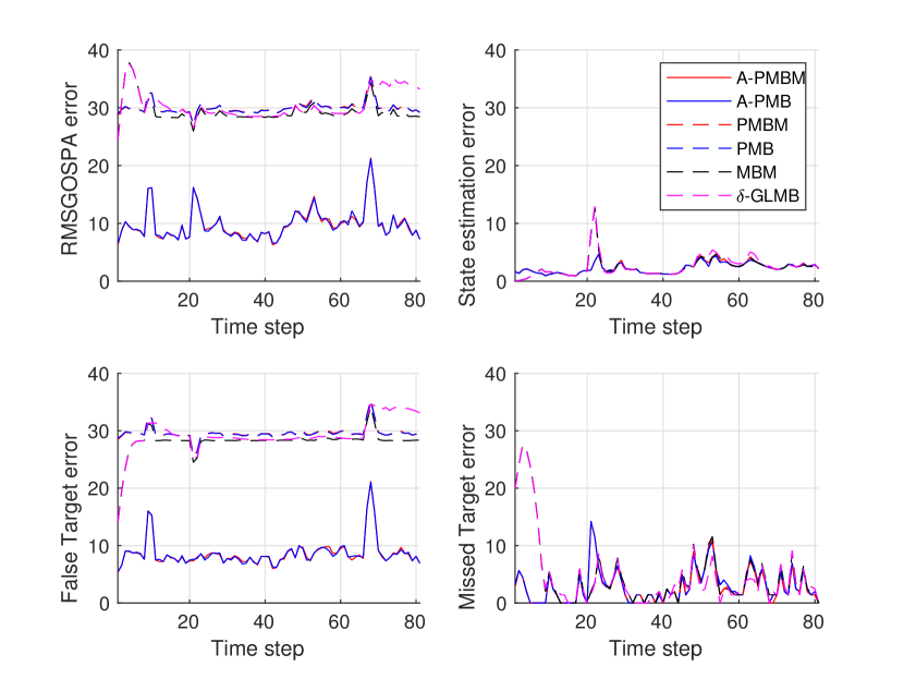
Figure 5: RMS GOSPA errors and their decomposition against time for the extended target scenario. A-PMBM and A-PMB perform considerably better than PMBM and PMB filters.

VI Conclusions

This paper has proved that, regardless of the distribution of the target-generated measurements and the clutter, the posterior is a PMBM for the standard multi-target dynamic models with PPP birth. This result implies that, if the birth model is instead multi-Bernoulli, the posterior is MBM, which can be labelled, and also written in MBM₀₁/$\delta$-GLMB form. We have also developed an implementation of the PMBM filter, and the corresponding PMB filter, for point targets and arbitrary clutter based on Gibbs sampling to obtain meaningful data association hypotheses.

We have evaluated the filter in two scenarios. First, we present a point-target scenario in which clutter is an IID cluster process with negative binomial cardinality distribution, we show the performance benefits of the A-PMBM and A-PMB filters compared with filters with PPP clutter. Second, we present the performance benefits of the A-PMBM and A-PMB filters in an extended-target scenario in which clutter is the union of a PPP process plus a number of independent sources of clutter.

Given the generality of the measurement model, there are many lines of future work, for example, developing specific models for target-generated measurements and clutter tailored to different applications, estimating their parameters, and implementing the corresponding PMBM/PMB/MBM/MB filters. It is also direct to extend these results to the multi-sensor case. Another line of future work is the implementation of these filters for a large number of targets, which usually requires the use of clustering and efficient data structures [4, 56, 57, 58].

Supplemental material: “Poisson multi-Bernoulli mixture filter with general target-generated measurements and arbitrary clutter”

Appendix A

This appendix proves the general PMBM filter update in Theorem 1 using probability generating functionals (PGFLs) [6]. In Section A-A, we first write the PGFLs of the prior and the measurements given the multi-target state. The joint PGFL of the prior and the measurements is derived in Section A-B. Finally, the PGFL of the posterior and the resulting posterior are derived in Section A-C.

A-A PGFLs of prior and measurements

Let $h\left(\cdot\right)$ be a unitless, real-valued function in the single-target space, and $h^{X}=\prod_{x\in X}h(x)$ with $h^{\emptyset}=1$. Then, the PGFL of the PMBM in (3) is [16]

$$G_{k|k^{\prime}}[h] =\int h^{X}f_{k|k^{\prime}}\left(X\right)\delta X,$$ (60)

$$G_{k|k^{\prime}}[h] =G_{k|k^{\prime}}^{\mathrm{p}}[h]\cdot G_{k|k^{\prime}}^{\mathrm{mbm}}[h],$$ (61)

$$G_{k|k^{\prime}}^{\mathrm{p}}[h] =\exp\left(\langle\lambda_{k|k^{\prime}},h-1\rangle\right)\propto\exp\left(\langle\lambda_{k|k^{\prime}},h\rangle\right),$$ (62)

$$G_{k|k^{\prime}}^{\mathrm{mbm}}[h] =\sum_{a\in\mathcal{A}_{k^{\prime}|k}}w_{k|k^{\prime}}^{a}\prod_{i=1}^{n_{k^{\prime}|k}}G_{k|k^{\prime}}^{i,a^{i}}[h]$$ (63)

$$\propto\sum_{a\in\mathcal{A}_{k^{\prime}|k}}w_{k|k^{\prime}}^{0,a^{0}}\prod_{i=1}^{n_{k|k^{\prime}}}\left[w_{k|k^{\prime}}^{i,a^{i}}G_{k|k^{\prime}}^{i,a^{i}}[h]\right]$$ (64)

where

$$G_{k|k^{\prime}}^{i,a^{i}}[h] =1-r_{k|k^{\prime}}^{i,a^{i}}+r_{k|k^{\prime}}^{i,a^{i}}\langle p_{k|k^{\prime}}^{i,a^{i}},h\rangle.$$ (65)

Given the multi-target state $X$, measurements from each target are independent, and there is also independent clutter. Therefore, the PGFL $M_{Z}[g|X]$ of the measurements given $X$ is the product of PGFLs

$$M_{Z}[g|X] =M_{C}[g]\prod_{x\in X}M_{T}[g|x]$$ (66)

where $M_{T}[g|x]$ is the PGFL of $f\left(\cdot|x\right)$, $M_{C}[g]$ is the PGFL of $c\left(\cdot\right)$, and $g\left(\cdot\right)$ is a unitless, real-valued function in the single-measurement space.

A-B Joint PGFL

The joint PGFL of the joint density of the set of measurements and set of targets is [16, 6]

$$F[g,h] =\int\int g^{Z_{k}}h^{X_{k}}f\left(Z_{k}|X_{k}\right)f_{k|k-1}\left(X_{k}\right)\delta Z_{k}\delta X_{k}$$

$$=\int M_{Z}[g|X_{k}]h^{X_{k}}f_{k|k-1}\left(X_{k}\right)\delta X_{k}$$ (67)

$$=M_{C}[g]G_{k|k-1}[hM_{T}[g|\cdot]]$$ (68)

$$\propto\exp\left(\langle\lambda_{k|k-1},hM_{T}[g|\cdot]\rangle\right)M_{C}[g]\sum_{a\in\mathcal{A}_{k|k-1}}w_{k|k-1}^{0,a^{0}}$$

$$\times\prod_{i=1}^{n_{k|k-1}}\left[w_{k|k-1}^{i,a^{i}}G_{k|k-1}^{i,a^{i}}\big{[}hM_{T}[g|\cdot]\big{]}\right].$$ (69)

We denote the first factor in (69) as

$$F^{0}[g,h] =\exp\left(\langle\lambda_{k|k-1},hM_{T}[g|\cdot]\rangle\right)$$ (70)

which represents the joint PGFL of measurements (not including clutter) and targets in the PPP, up to a proportionality constant. We also denote

$$F^{i,a^{i}}[g,h] =G_{k|k-1}^{i,a^{i}}\big{[}hM_{T}[g|\cdot]\big{]}$$ (71)

$$=1-r_{k|k-1}^{i,a^{i}}+r_{k|k-1}^{i,a^{i}}\bigg{\langle}p_{k|k-1}^{i,a^{i}},hM_{T}[g|\cdot]\bigg{\rangle},$$ (72)

which is the joint PGFL of measurements (not including clutter) and the $i$-th target. Then, we can write (69) as

$$F[g,h] \propto F^{0}[g,h]M_{C}[g]$$

$$\times\sum_{a\in\mathcal{A}_{k|k-1}}w_{k|k-1}^{0,a^{0}}\prod_{i=1}^{n_{k|k-1}}\left[w_{k|k-1}^{i,a}F^{i,a^{i}}[g,h]\right].$$ (73)

A-C Updated PGFL

We proceed to calculate the PGFL $G_{k|k}[h]$ of the updated density $f_{k|k}\left(\cdot\right)$. This PGFL can be calculated by the set derivative of $F[g,h]$ w.r.t. $Z_{k}$ evaluated at $g=0$ [6, Sec. 5.8][16, Eq. (25)]

$$G_{k|k}[h] \propto\frac{\delta}{\delta Z_{k}}F[g,h]\bigg{|}_{g=0}.$$ (74)

Substituting (73) into (74) and applying the product rule for sets derivatives [6, Eq. (3.68)], we obtain

$$G_{k|k}[h]$$

$$\propto\sum_{W^{C}\uplus W_{0}\uplus\cdots\uplus W_{n_{k|k-1}}=Z_{k}}\frac{\delta}{\delta W^{C}}M_{C}[g]\frac{\delta}{\delta W_{0}}F^{0}[g,h]$$

$$\times\sum_{a\in\mathcal{A}_{k|k-1}}w_{k|k-1}^{0,a^{0}}\prod_{i=1}^{n_{k|k-1}}\frac{\delta}{\delta W_{i}}\left(w_{k|k-1}^{i,a^{i}}F^{i,a^{i}}[g,h]\right)\bigg{|}_{g=0}.$$ (75)

In the first sum in (75), we decompose the measurement set $Z_{k}$ into $n_{k|k-1}+2$ subsets. The subset $W^{C}$ represents measurements that are considered clutter, the subset $W_{0}$ represents measurements that are the first detection of an undetected target (modelled in the PPP), and subset $W_{i}$, $i>0$, represents measurements assigned to the $i$-th predicted Bernoulli component. We proceed to calculate the required set derivatives.

A-C1 Set derivative w.r.t. $W^{C}$ (clutter weight)

As $M_{C}[g]$ is the PGFL of $c\left(\cdot\right)$, we can directly see by the properties of the set derivative of a PGFL [6, Sec. 3.5.1] that

$$\frac{\delta}{\delta W^{C}}M_{C}[g]\bigg{|}_{g=0} =c\left(W^{C}\right).$$ (76)

A-C2 Set derivative w.r.t. $W_{0}$ (PPP update)

We calculate

$$\frac{\delta}{\delta W_{0}}F^{0}[g,h]\bigg{|}_{g=0}.$$

This corresponds to the PGFL in [19, Eq. (84)] setting the clutter intensity equal to zero. Therefore, following [19, Lem. 4], we obtain

$$\frac{\delta}{\delta W_{0}}F^{0}[g,h] =F^{0}[g,h]\sum_{P\angle W_{0}}\prod_{V\in P}d_{V}[g,h]$$ (77)

where

$$d_{V}[g,h]=\frac{\delta}{\delta V}\left(\big{\langle}\lambda_{k|k-1},hM_{T}[g|\cdot]\big{\rangle}\right)$$ (78)

and $\sum_{P\angle W_{0}}$ denotes the sum over all partitions $P$ of $W_{0}$.

We evaluate the first factor in (77), $F^{0}[g,h]$, at $g=0$ resulting in

$$F^{0}[0,h] =\exp\left(\big{\langle}\lambda_{k|k-1},hf\left(\emptyset|\cdot\right)\big{\rangle}\right)$$ (79)

where we have used that $M_{T}[0|\cdot]=f\left(\emptyset|\cdot\right)$. This is proportional to the PGFL of a PPP with intensity (9). Then, the following lemma indicates the distributions resulting from evaluating (78) at $g=0$. The lemma is obtained by setting the clutter intensity to zero in [19, Lem. 5].

Lemma 4.

The update of the PGFL of the PPP prior with measurement subset $V$, $|V|>0$,

$$w_{k|k}^{V}G_{k|k}^{V}[h]=d_{V}[g,h]\Big{|}_{g=0}$$

are PGFLs of weighted Bernoulli distributions with the form [16, Lem. 2]

$$f_{k|k}^{V}(X)=w_{k|k}^{V}\times\begin{cases}1-r_{k|k}^{V}&X=\emptyset\\ r_{k|k}^{V}p_{k|k}^{V}(x)&X=\{x\}\\ 0&\left|X\right|>1\end{cases}$$ (80)

where

$$w_{k|k}^{V} =l_{k|k}^{V},$$ (81)

$$l_{k|k}^{V} =\bigg{\langle}\lambda_{k|k-1},f\left(V|\cdot\right)\bigg{\rangle},$$ (82)

$$r_{k|k}^{V} =\frac{l_{k|k}^{V}}{w_{k|k}^{V}}=1,$$ (83)

$$p_{k|k}^{V}(x) =\frac{f\left(V|x\right)\lambda_{k|k-1}\left(x\right)}{l_{k|k}^{V}}.\quad\square$$ (84)

This lemma indicates how to create the new Bernoulli components in Theorem 1.

A-C3 Set derivative w.r.t. $W_{i}$ (Bernoulli update)

The third factor is analogous to the one in [19, App. A.C.1], which yields

$$\frac{\delta}{\delta W_{i}}F^{i,a^{i}}[g,h]\bigg{|}_{g=0} =\begin{cases}F^{i,a^{i}}[g,h]&W_{i}=\emptyset\\ r_{k|k-1}^{i,a^{i}}\Big{\langle}f_{k|k-1}^{i,a^{i}},hf\left(W_{i}|\cdot\right)\Big{\rangle}&W_{i}\neq\emptyset.\end{cases}$$ (85)

As shown in [16, Lem. 2], this equation represents weighted Bernoulli densities with the parameters indicated in Theorem 1 (update of previous Bernoulli), see also [19, Lem. 3].

A-C4 Final expression

Substituting (76), (77) and (85) into (75), we obtain

$$G_{k|k}[h]$$

$$\propto F^{0}[0,h]\sum_{W^{C}\uplus W_{0}\uplus\cdots\uplus W_{n_{k|k-1}}=Z_{k}}c\left(W^{C}\right)$$

$$\times\sum_{P\angle W_{0}}\prod_{V\in P}w_{k|k}^{V}G_{k|k}^{V}[h]$$

$$\times\sum_{a\in\mathcal{A}_{k|k-1}}w_{k|k-1}^{0,a^{0}}\prod_{i=1}^{n_{k|k-1}}\left(w_{k|k-1}^{i,a^{i}}\frac{\delta}{\delta W_{i}}F^{i,a^{i}}[g,h]\bigg{|}_{g=0}\right).$$ (86)

In this expression, $F^{0}[0,h]$ represents the PPP of undetected targets with intensity (9). Then, for each predicted global hypothesis, we generate a new global hypotheses by partitioning the measurements into $W^{C},W_{0},\cdots,W_{n_{k|k-1}}$ and going through the partitions of $W_{0}.$ The weight of the clutter hypothesis is given by $c\left(W^{C}\right)w_{k|k-1}^{0,a^{0}}$, which results in (10) and (12). Then, for each new global hypothesis, we have a multi-Bernoulli, where the previous Bernoulli densities are updated as in (13)-(21), and the new Bernoulli components as in (24)-(25). We then finish the proof of Theorem 1, by writing the updated density in a track-oriented form.

Appendix B

In this appendix, we write the expression of the PMBM update when clutter is the union of Poisson clutter and $n_{c}$ independent sources of clutter. That is, the clutter density is

$$c\left(Z_{c}\right) =\sum_{\uplus_{l=0}^{n_{c}}Z^{l}=Z_{c}}c^{0}\left(Z^{0}\right)\prod_{i_{c}=1}^{n_{c}}c^{i_{c}}\left(Z^{i_{c}}\right)$$ (87)

where

$$c^{0}\left(Z^{0}\right) =e^{-\int\lambda^{C}\left(z\right)dz}\prod_{z\in Z^{0}}\lambda^{C}\left(z\right)$$

where $c^{0}\left(\cdot\right)$ is the density of the PPP clutter with intensity $\lambda^{C}\left(\cdot\right)$, and $c^{i_{c}}\left(\cdot\right)$ is the density of the $i_{c}$ source of clutter.

We can directly use Theorem 1 to obtain the updated PMBM density. With this approach, we consider a single local hypothesis with clutter measurements. If the clutter density has form (87), we can alternatively define a local hypothesis $a^{i}\in\left\{1,...,h_{k|k^{\prime}}^{i}\right\}$ for each Bernoulli component $i>0$, and also a local hypothesis $a^{0,i_{c}}\in\left\{1,...,h_{k|k^{\prime}}^{0,i_{c}}\right\}$ for the $i$-th clutter source. A global hypothesis is $a=\left(a^{0,1},...,a^{0,n_{c}},a^{1},...,a^{n_{k|k^{\prime}}}\right)\in\mathcal{A}_{k|k^{\prime}}$, where $\mathcal{A}_{k|k^{\prime}}$ is the set of global hypotheses. That is, as in PMBM filters with PPP clutter, the [16, 18, 19], the creation of new Bernoulli components will take into account the PPP clutter, and then, we also have additional sources of clutter.

The weight of a global hypothesis $a$ is

$$w_{k|k^{\prime}}^{a}\propto\prod_{i_{c}=1}^{n_{c}}w_{k|k^{\prime}}^{0,i_{c},a^{0,i_{c}}}\prod_{i=1}^{n_{k|k^{\prime}}}w_{k|k^{\prime}}^{i,a^{i}}.$$ (88)

At time step zero, the filter is initiated with $n_{0|0}=0$, $w_{0|0}^{0,i_{c}}=1$, $h_{0|0}^{0,i_{c}}=1$, $\mathcal{M}_{0}^{0,i_{c}}=\emptyset$. The update is provided in the following theorem.

Theorem 5.

Assume the predicted density $f_{k|k-1}\left(\cdot\right)$ is a PMBM of the form (3). Then, the updated density $f_{k|k}\left(\cdot\right)$ with set $Z_{k}=\left\{z_{k}^{1},...,z_{k}^{m_{k}}\right\}$ is a PMBM with the following parameters. The number of Bernoulli components is $n_{k|k}=n_{k|k-1}+2^{m_{k}}-1$. The intensity of the PPP is

$$\lambda_{k|k}\left(x\right) =f\left(\emptyset|x\right)\lambda_{k|k-1}\left(x\right).$$ (89)

Let $Z_{k}^{1},...,Z_{k}^{2^{m_{k}}-1}$ be the non-empty subsets of $Z_{k}$. The number of updated local clutter hypotheses for the $i_{c}$-th clutter source is $h_{k|k}^{0,i_{c}}=2^{m_{k}}h_{k|k-1}^{0,i_{c}}$ such that a new local clutter hypothesis is included for each previous local clutter hypothesis and either a misdetection or an update with a non-empty subset of $Z_{k}$. The updated local hypothesis with 0 measurements for the $i$-th clutter source, $a^{0,i_{c}}\in\left\{1,...,h_{k|k-1}^{0,i_{c}}\right\}$, has parameters

$$\mathcal{M}_{k}^{0,i_{c},a^{0,i_{c}}} =\mathcal{M}_{k-1}^{0,i_{c},a^{0}},$$

$$w_{k|k}^{0,i_{c},a^{0,i_{c}}} =w_{k|k-1}^{0,i_{c},a^{0,i_{c}}}c^{i_{c}}\left(\emptyset\right).$$

For a previous local clutter hypothesis $\widetilde{a}^{0,i_{c}}\in\left\{1,...,h_{k|k-1}^{0,i_{c}}\right\}$ for the $i_{c}$ clutter source in the predicted density, the new local clutter hypothesis generated by a a set $Z_{k}^{j}$ has $a^{0,i_{c}}=\widetilde{a}^{0,i_{c}}+h_{k|k-1}^{0,i_{c}}j$,

$$\mathcal{M}_{k}^{0,i_{c},a^{0,i_{c}}} =\mathcal{M}_{k-1}^{0,i_{c},\widetilde{a}^{0,i_{c}}}\cup\left\{\left(k,p\right):z_{k}^{p}\in Z_{k}^{j}\right\},$$

$$w_{k|k}^{0,i_{c},a^{0,i_{c}}} =w_{k|k-1}^{0,i_{c},a^{0,i_{c}}}c^{i_{c}}\left(Z_{k}^{j}\right).$$

For Bernoulli components continuing from previous time steps $i\in\left\{1,...,n_{k|k-1}\right\}$, a new local hypothesis is included for each previous local hypothesis and either a misdetection or an update with a non-empty subset of $Z_{k}$. The updated number of local hypotheses is $h_{k|k}^{i}=2^{m_{k}}h_{k|k-1}^{i}$. For missed detection hypotheses, $i\in\left\{1,...,n_{k|k-1}\right\}$, $a^{i}\in\left\{1,...,h_{k|k-1}^{i}\right\}$, we obtain

$$\mathcal{M}_{k}^{i,a^{i}} =\mathcal{M}_{k-1}^{i,a^{i}},$$ (90)

$$l_{k|k}^{i,a^{i},\emptyset} =\big{\langle}f_{k|k-1}^{i,a^{i}},f\left(\emptyset|\cdot\right)\big{\rangle},$$ (91)

$$w_{k|k}^{i,a^{i}} =w_{k|k-1}^{i,a^{i}}\left[1-r_{k|k-1}^{i,a^{i}}+r_{k|k-1}^{i,a^{i}}l_{k|k}^{i,a^{i},\emptyset}\right],$$ (92)

$$r_{k|k}^{i,a^{i}} =\frac{r_{k|k-1}^{i,a^{i}}l_{k|k}^{i,a^{i},\emptyset}}{1-r_{k|k-1}^{i,a^{i}}+r_{k|k-1}^{i,a^{i}}l_{k|k}^{i,a^{i},\emptyset}},$$ (93)

$$f_{k|k}^{i,a^{i}}(x) =\frac{f\left(\emptyset|x\right)f_{k|k-1}^{i,a^{i}}(x)}{l_{k|k}^{i,a^{i},\emptyset}}.$$ (94)

Let $Z_{k}^{1},...,Z_{k}^{2^{m_{k}}-1}$ be the non-empty subsets of $Z_{k}$. For a Bernoulli component $i\in\left\{1,...,n_{k|k-1}\right\}$ with a local hypothesis $\widetilde{a}^{i}\in\left\{1,...,h_{k|k-1}^{i}\right\}$ in the predicted density, the new local hypothesis generated by a set $Z_{k}^{j}$ has $a^{i}=\widetilde{a}^{i}+h_{k|k-1}^{i}j$, $r_{k|k}^{i,a^{i}}=1$, and

$$\mathcal{M}_{k}^{i,a^{i}} =\mathcal{M}_{k-1}^{i,\widetilde{a}^{i}}\cup\left\{\left(k,p\right):z_{k}^{p}\in Z_{k}^{j}\right\},$$ (95)

$$l_{k|k}^{i,a^{i},Z_{k}^{j}} =\bigg{\langle}f_{k|k-1}^{i,\widetilde{a}^{i}},f\left(Z_{k}^{j}|\cdot\right)\bigg{\rangle},$$ (96)

$$w_{k|k}^{i,a^{i}} =w_{k|k-1}^{i,\widetilde{a}^{i}}r_{k|k-1}^{i,\widetilde{a}^{i}}l_{k|k}^{i,a^{i},Z_{k}^{j}},$$ (97)

$$f_{k|k}^{i,a^{i}}(x) =\frac{f\left(Z_{k}^{j}|x\right)f_{k|k-1}^{i,\widetilde{a}^{i}}(x)}{l_{k|k}^{i,a^{i},Z_{k}^{j}}}.$$ (98)

For the new Bernoulli component initiated by subset $Z_{k}^{j}$, whose index is $i=n_{k|k-1}+j$, we have two local hypotheses ($h_{k|k}^{i}=2$), one corresponding to a non-existent Bernoulli density

$$\mathcal{M}_{k}^{i,1}=\emptyset,\;w_{k|k}^{i,1}=1,\;r_{k|k}^{i,1}=0,$$ (99)

and the other with

$$\mathcal{M}_{k}^{i,2} =\left\{\left(k,p\right):z_{k}^{p}\in Z_{k}^{j}\right\},$$ (100)

$$l_{k|k}^{Z_{k}^{j}} =\bigg{\langle}\lambda_{k|k-1},f\left(Z_{k}^{j}|\cdot\right)\bigg{\rangle},$$ (101)

$$w_{k|k}^{i,2} =\delta_{1}\left[|Z_{k}^{j}|\right]\left[\prod_{z\in Z_{k}^{j}}\lambda^{C}\left(z\right)\right]+l_{k|k}^{Z_{k}^{j}},$$ (102)

$$r_{k|k}^{i,2} =\frac{l_{k|k}^{Z_{k}^{j}}}{w_{k|k}^{i,a^{i}}},$$ (103)

$$f_{k|k}^{i,2}(x) =\frac{f\left(Z_{k}^{j}|x\right)\lambda_{k|k-1}(x)}{l_{k|k}^{Z_{k}^{j}}}.\quad\square$$ (104)

The proof is equivalent to the one of Theorem 1 in Appendix A, but adding $n_{c}$ sources of clutter and a PPP clutter source. The PPP clutter source is incorporated in the update for new Bernoulli components as in [19]. The main differences with Theorem 1 are that now there are updates with detection and misdetection hypotheses with the $n_{c}$ clutter sources, and that the intensity of the clutter affects (102). This implies that the probability of existence for new Bernoulli components can be lower than 1. It should be noted that if in Theorem 5, we set $n_{c}=1$ and $\lambda^{C}\left(\cdot\right)=0$, we recover Theorem 1.

References

- [1] S. Blackman and R. Popoli, Design and Analysis of Modern Tracking Systems. Artech House, 1999.
- [2] P. Held, D. Steinhauser, A. Koch, T. Brandmeier, and U. T. Schwarz, “A novel approach for model-based pedestrian tracking using automotive radar,” IEEE Transactions on Intelligent Transportation Systems, vol. 23, no. 7, pp. 7082–7095, 2022.
- [3] A. Buelta, A. Olivares, E. Staffetti, W. Aftab, and L. Mihaylova, “A Gaussian process iterative learning control for aircraft trajectory tracking,” IEEE Transactions on Aerospace and Electronic Systems, vol. 57, no. 6, pp. 3962–3973, 2021.
- [4] D. Reid, “An algorithm for tracking multiple targets,” IEEE Transactions on Automatic Control, vol. 24, no. 6, pp. 843–854, Dec. 1979.
- [5] Y. Bar-Shalom and E. Tse, “Tracking in a cluttered environment with probabilistic data association,” Automatica, vol. 11, no. 5, pp. 451–460, 1975.
- [6] R. P. S. Mahler, Advances in Statistical Multisource-Multitarget Information Fusion. Artech House.
- [7] M. S. Greco and S. Watts, “Radar clutter modeling and analysis,” in Academic Press Library in Signal Processing, N. D. Sidiropoulos, F. Gini, R. Chellappa, and S. Theodoridis, Eds. Elsevier, 2014, vol. 2, pp. 513–594.
- [8] M. Skolnik, Introduction to Radar Systems. McGraw-Hill, 2001.
- [9] Ø. K. Helgesen, K. Vasstein, E. F. Brekke, and A. Stahl, “Heterogeneous multi-sensor tracking for an autonomous surface vehicle in a littoral environment,” Ocean Engineering, vol. 252, pp. 1–16, 2022.
- [10] H. Cho, Y. Seo, B. V. K. V. Kumar, and R. R. Rajkumar, “A multi-sensor fusion system for moving object detection and tracking in urban driving environments,” in IEEE International Conference on Robotics and Automation, 2014, pp. 1836–1843.
- [11] S. Scheidegger, J. Benjaminsson, E. Rosenberg, A. Krishnan, and K. Granström, “Mono-camera 3D multi-object tracking using deep learning detections and PMBM filtering,” in IEEE Intelligent Vehicles Symposium, 2018, pp. 433–440.
- [12] J. Zhao, P. Wu, X. Liu, Y. Xu, L. Mihaylova, S. Godsill, and W. Wang, “Audio-visual tracking of multiple speakers via a PMBM filter,” in IEEE International Conference on Acoustics, Speech and Signal Processing, 2022, pp. 5068–5072.
- [13] G. R. Mellema, “Improved active sonar tracking in clutter using integrated feature data,” IEEE Journal of Oceanic Engineering, vol. 45, no. 1, pp. 304–318, 2020.
- [14] D. Grimmett, D. Abraham, and R. Alberto, “Cognitive active sonar tracking for optimum performance in clutter,” in 24th International Conference on Information Fusion, 2021, pp. 1–8.
- [15] O. Erdinc, P. Willett, and Y. Bar-Shalom, “The bin-occupancy filter and its connection to the PHD filters,” IEEE Transactions on Signal Processing, vol. 57, no. 11, pp. 4232–4246, Nov. 2009.
- [16] J. L. Williams, “Marginal multi-Bernoulli filters: RFS derivation of MHT, JIPDA and association-based MeMBer,” IEEE Transactions on Aerospace and Electronic Systems, vol. 51, no. 3, pp. 1664–1687, July 2015.
- [17] A. F. García-Fernández, J. L. Williams, K. Granström, and L. Svensson, “Poisson multi-Bernoulli mixture filter: direct derivation and implementation,” IEEE Transactions on Aerospace and Electronic Systems, vol. 54, no. 4, pp. 1883–1901, Aug. 2018.
- [18] K. Granström, M. Fatemi, and L. Svensson, “Poisson multi-Bernoulli mixture conjugate prior for multiple extended target filtering,” IEEE Transactions on Aerospace and Electronic Systems, vol. 56, no. 1, pp. 208–225, Feb. 2020.
- [19] A. F. García-Fernández, J. L. Williams, L. Svensson, and Y. Xia, “A Poisson multi-Bernoulli mixture filter for coexisting point and extended targets,” IEEE Transactions on Signal Processing, vol. 69, pp. 2600–2610, 2021.
- [20] K. Granström, M. Baum, and S. Reuter, “Extended object tracking:introduction, overview, and applications,” Journal of Advances in Information Fusion, vol. 12, no. 2, pp. 139–174, Dec. 2017.
- [21] B. N. Vo, B. T. Vo, and H. G. Hoang, “An efficient implementation of the generalized labeled multi-Bernoulli filter,” IEEE Transactions on Signal Processing, vol. 65, no. 8, pp. 1975–1987, April 2017.
- [22] M. Beard, S. Reuter, K. Granström, B.-T. Vo, B.-N. Vo, and A. Scheel, “Multiple extended target tracking with labeled random finite sets,” IEEE Transactions on Signal Processing, vol. 64, no. 7, pp. 1638–1653, 2016.
- [23] S. Watts, “Radar sea clutter: Recent progress and future challenges,” in International Conference on Radar, 2008, pp. 10–16.
- [24] X. Shen, Z. Song, H. Fan, and Q. Fu, “General Bernoulli filter for arbitrary clutter and target measurement processes,” IEEE Signal Processing Letters, vol. 25, no. 10, pp. 1525–1529, Oct. 2018.
- [25] D. Clark and R. Mahler, “Generalized PHD filters via a general chain rule,” in 15th International Conference on Information Fusion, July 2012, pp. 157–164.
- [26] X. Shen, L. Zhang, M. Hu, S. Xiao, and H. Tao, “Arbitrary clutter extended target probability hypothesis density filter,” IET Radar, Sonar & Navigation, vol. 15, no. 5, pp. 510–522, 2021.
- [27] I. Schlangen, E. Delande, J. Houssineau, and D. E. Clark, “A PHD filter with negative binomial clutter,” in 19th International Conference on Information Fusion, 2016, pp. 658–665.
- [28] I. Schlangen, E. D. Delande, J. Houssineau, and D. E. Clark, “A second-order PHD filter with mean and variance in target number,” IEEE Transactions on Signal Processing, vol. 66, no. 1, pp. 48–63, 2018.
- [29] D. E. Clark and F. De Melo, “A linear-complexity second-order multi-object filter via factorial cumulants,” in 21st International Conference on Information Fusion, 2018, pp. 1250–1259.
- [30] M. A. Campbell, D. E. Clark, and F. de Melo, “An algorithm for large-scale multitarget tracking and parameter estimation,” IEEE Transactions on Aerospace and Electronic Systems, vol. 57, no. 4, pp. 2053–2066, 2021.
- [31] X. Shen, L. Zhang, M. Hu, S. Xiao, and H. Tao, “A general cardinalized probability hypothesis density filter,” EURASIP Journal on Advances in Signal Processing, vol. 94, pp. 1–31, 2022.
- [32] R. Mahler, “A clutter-agnostic generalized labeled multi-Bernoulli filter,” in Proceedings of SPIE Signal Processing, Sensor/Information Fusion, and Target Recognition XXVII, 2018, pp. 1–12.
- [33] A. F. García-Fernández, L. Svensson, J. L. Williams, Y. Xia, and K. Granström, “Trajectory Poisson multi-Bernoulli filters,” IEEE Transactions on Signal Processing, vol. 68, pp. 4933–4945, 2020.
- [34] C. Hue, J.-P. Le Cadre, and P. Perez, “Tracking multiple objects with particle filtering,” IEEE Transactions on Aerospace and Electronic Systems, vol. 38, no. 3, pp. 791–812, Jul 2002.
- [35] ——, “Sequential Monte Carlo methods for multiple target tracking and data fusion,” IEEE Transactions on Signal Processing, vol. 50, no. 2, pp. 309–325, 2002.
- [36] K. Granström, L. Svensson, S. Reuter, Y. Xia, and M. Fatemi, “Likelihood-based data association for extended object tracking using sampling methods,” IEEE Transactions on Intelligent Vehicles, vol. 3, no. 1, pp. 30–45, March 2018.
- [37] K. Granström, C. Lundquist, and O. Orguner, “Extended target tracking using a Gaussian-mixture PHD filter,” IEEE Transactions on Aerospace and Electronic Systems, vol. 48, no. 4, pp. 3268–3286, Oct. 2012.
- [38] K. Gilholm, S. Godsill, S. Maskell, and D. Salmond, “Poisson models for extended and group tracking,” in Proc. SPIE 5913, Signal and Data Processing of Small Targets, vol. 5913, 2005, pp. 1–12.
- [39] M. B. Porter, “Beam tracing for two- and three-dimensional problems in ocean acoustics,” The Journal of the Acoustical Society of America, vol. 146, pp. 2016–2029, 2019.
- [40] Y. Ge, H. Kim, F. Wen, L. Svensson, S. Kim, and H. Wymeersch, “Exploiting diffuse multipath in 5G SLAM,” in IEEE Global Communications Conference, 2020, pp. 1–6.
- [41] A. Narykov, M. Wright, Á. F. García-Fernández, S. Maskell, and J. F. Ralph, “Poisson multi-Bernoulli mixture filtering with an active sonar using BELLHOP simulation,” in 25th International Conference on Information Fusion, 2022, pp. 1–7.
- [42] W. Si, H. Zhu, and Z. Qu, “Robust Poisson multi-Bernoulli filter with unknown clutter rate,” IEEE Access, vol. 7, pp. 117 871–117 882, 2019.
- [43] Y. Xia, K. Granström, L. Svensson, M. Fatemi, A. F. García-Fernández, and J. L. Williams, “Poisson multi-Bernoulli approximations for multiple extended object filtering,” IEEE Transactions on Aerospace and Electronic Systems, vol. 58, no. 2, pp. 890–906, 2022.
- [44] D. Franken, M. Schmidt, and M. Ulmke, “"Spooky action at a distance" in the cardinalized probability hypothesis density filter,” IEEE Transactions on Aerospace and Electronic Systems, vol. 45, no. 4, pp. 1657–1664, Oct. 2009.
- [45] J. L. Williams, “An efficient, variational approximation of the best fitting multi-Bernoulli filter,” IEEE Transactions on Signal Processing, vol. 63, no. 1, pp. 258–273, Jan. 2015.
- [46] K. G. Murty, “An algorithm for ranking all the assignments in order of increasing cost.” Operations Research, vol. 16, no. 3, pp. 682–687, 1968.
- [47] D. F. Crouse, “On implementing 2D rectangular assignment algorithms,” IEEE Transactions on Aerospace and Electronic Systems, vol. 52, no. 4, pp. 1679–1696, August 2016.
- [48] J. S. Liu, Monte Carlo Strategies in Scientific Computing. Springer, 2001.
- [49] M. Zhou and L. Carin, “Negative binomial process count and mixture modeling,” IEEE Transactions on Pattern Analysis and Machine Intelligence, vol. 37, no. 2, pp. 307–320, 2015.
- [50] A. F. García-Fernández, Y. Xia, K. Granström, L. Svensson, and J. L. Williams, “Gaussian implementation of the multi-Bernoulli mixture filter,” in Proceedings of the 22nd International Conference on Information Fusion, 2019.
- [51] B.-N. Vo and W.-K. Ma, “The Gaussian mixture probability hypothesis density filter,” IEEE Transactions on Signal Processing, vol. 54, no. 11, pp. 4091–4104, Nov. 2006.
- [52] Y. Bar-Shalom, T. Kirubarajan, and X. R. Li, Estimation with Applications to Tracking and Navigation. John Wiley & Sons, Inc., 2001.
- [53] A. S. Rahmathullah, A. F. García-Fernández, and L. Svensson, “Generalized optimal sub-pattern assignment metric,” in 20th International Conference on Information Fusion, 2017, pp. 1–8.
- [54] M. Ester, H.-P. Kriegel, J. Sander, and X. Xu, “A density-based algorithm for discovering clusters in large spatial datasets with noise,” in 2nd International Conference on Knowledge Discovery and Data Mining, 1996, pp. 226–231.
- [55] S. Yang, M. Baum, and K. Granström, “Metrics for performance evaluation of elliptic extended object tracking methods,” in IEEE International Conference on Multisensor Fusion and Integration for Intelligent Systems, 2016, pp. 523–528.
- [56] M. Fontana, A. F. García-Fernández, and S. Maskell, “Data-driven clustering and Bernoulli merging for the Poisson multi-Bernoulli mixture filter,” accepted in IEEE Transactions on Aerospace and Electronic Systems, 2023.
- [57] M. Beard, B. T. Vo, and B. Vo, “A solution for large-scale multi-object tracking,” IEEE Transactions on Signal Processing, vol. 68, pp. 2754–2769, 2020.
- [58] J. Roy, N. Duclos-Hindie, and D. Dessureault, “Efficient cluster management algorithm for multiple hypothesis tracking,” in Proc. SPIE Signal and Data Processing of Small Targets, 1997, pp. 301–313.