de Sitter space, extremal surfaces
and “time-entanglement”

K. Narayan

Chennai Mathematical Institute,
H1 SIPCOT IT Park, Siruseri 603103, India.

We refine previous investigations on de Sitter space and extremal surfaces anchored at the future boundary $I^{+}$. Since such surfaces do not return, they require extra data or boundary conditions in the past (interior). In entirely Lorentzian de Sitter spacetime, this leads to future-past timelike surfaces stretching between $I^{\pm}$. Apart from an overall $-i$ factor (relative to spacelike surfaces in $AdS$) their areas are real and positive. With a no-boundary type boundary condition, the top half of these timelike surfaces joins with a spacelike part on the hemisphere giving a complex-valued area. Motivated by these, we describe two aspects of “time-entanglement” in simple toy models in quantum mechanics. One is based on a future-past thermofield double type state entangling timelike separated states, which leads to entirely positive structures. Another is based on the time evolution operator and reduced transition amplitudes, which leads to complex-valued entropy.

1 Introduction and summary

It is of great interest to understand holography for de Sitter space (see the review [2]). In de Sitter (and cosmology more generally) perhaps the natural asymptotics are in the far future or the far past: this thinking leads to $dS/CFT$ [3, 4, 5] (and [6] in the higher spin context), which associates a hypothetical non-unitary dual Euclidean CFT at the future boundary $I^{+}$, with several dramatic differences from $AdS$ [7, 8, 9]. A particularly fascinating question is whether de Sitter entropy [10] can be understood as some sort of entanglement entropy. It is then natural to ask if the extensive investigations of holographic entanglement in $AdS$ [11, 12, 13] can be generalized to de Sitter space.

One possible generalization of the Ryu-Takayanagi formulation to de Sitter space is to consider the bulk analog of setting up entanglement entropy in the dual Euclidean $CFT$ on the future boundary [14]. We restrict to some boundary Euclidean time slice as a crutch, define subregions on these slices, and look for extremal surfaces anchored at $I^{+}$ dipping into the holographic (time) direction. Analysing this extremization interestingly shows that surfaces anchored at $I^{+}$ do not return to $I^{+}$, i.e. there is no $I^{+}\rightarrow I^{+}$ turning point, so there are no spacelike surfaces connecting points on $I^{+}$. There exist analytic continuations of RT surfaces in $AdS$ which lead to complex extremal surfaces [14, 15, 16, 17]. In [18, 19], entirely timelike future-past extremal surfaces were studied, stretching from $I^{+}$ to $I^{-}$.

In this note, we develop this further, stitching together an overall perspective which hopefully adds value to the understanding of these studies. The absence of $I^{+}\rightarrow I^{+}$ returns for surfaces implies that surfaces starting at $I^{+}$ continue inward, to the past: this suggests that they require extra data or boundary conditions in the interior, or far past to be well-defined. One obvious possibility for an entirely Lorentzian de Sitter space (sec. 2.1) is that the surfaces then end at the past boundary $I^{-}$. Analysing this in detail leads to future-past surfaces stated above [18, 19]. These are timelike extremal surfaces stretching between subregions at $I^{+}$ and equivalent ones at $I^{-}$: they are akin to rotated analogs of the Hartman-Maldacena surfaces [20] in the eternal $AdS$ black hole. Being entirely timelike, their area has an overall $-i$ factor, relative to the familiar spacelike extremal surfaces in $AdS$ (this overall $-i$ was discarded in [18, 19]; see below). Since we obtain codim-2 surfaces (when they exist), their area scales as de Sitter entropy.

Another possibility for the interior boundary conditions arises from modifying de Sitter from being entirely Lorentzian in accord with the Hartle-Hawking no-boundary prescription, i.e. to cut $dS$ in the middle and remove the bottom half, replacing it with a hemisphere (sec. 2.2). Now we join the top timelike part of the extremal surfaces above with regularity at the mid-slice to a spatial extremal surface that goes around the hemisphere (thus turning around): see [21, 22] for $dS_{3}$. This spacelike part has real area so that the total area is complex-valued. The top part of the surface (in the Lorentzian de Sitter) is the same as in the entirely timelike surfaces above: this reflects consistency of the future-past surfaces with Hartle-Hawking boundary conditions. The finite real part of the area of the no-boundary surfaces arises from the hemisphere and is precisely half de Sitter entropy for any dimension when the subregion at $I^{+}$ becomes maximal. In sec. 4, we give some comments on these future-past and no-boundary surface areas in terms of time contours, and argue that they can be regarded as space-time rotations from timelike subregions in $AdS$-like spaces.

Imaginary values also arise in studies of quantum extremal surfaces in de Sitter with regard to the future boundary [23, 24], stemming from timelike-separations (sec. 2.3). Complex-valued entanglement entropy was also found quite explicitly in studies of ghost-like theories, including simple toy quantum-mechanical models of “ghost-spins”, e.g. [25, 26].

For entirely Lorentzian $dS$, the entirely timelike future-past surfaces are akin to entirely timelike geodesics for ordinary particles moving in time. Removing the overall $-i$ in their pure imaginary areas (relative to real spacelike surface areas) is akin to calling the length of timelike geodesics as “time” rather than “$-i\cdot$space”. Overall this suggests that the areas of these $dS$ extremal surfaces with timelike components encode some new object, “time-entanglement”, distinct from usual spatial entanglement. In sec. 3, we describe two aspects of this in ordinary quantum mechanics, which incorporate this entry of late and early time boundary conditions. One is based on a future-past thermofield-double state [18] (see also [27, 28]) which leads to entirely positive structures despite the timelike separation. The other involves the time-evolution operator and “reduced transition amplitudes”, giving complex-valued entropy. As we were preparing this, the work [29] appeared with partial overlap.

2 $dS$ extremal surfaces from $I^{+}$, boundary conditions

The simplest place to see the absence of $I^{+}\rightarrow I^{+}$ turning points [14] is in the Poincare slicing with planar foliations, so

$$ds_{d+1}^{2}={R_{dS}^{2}\over\tau^{2}}(-d\tau^{2}+dy_{i}^{2})={R_{dS}^{2}\over\tau^{2}}(-d\tau^{2}+dw^{2}+dx_{i}^{2})\ .$$ (1)

Here we have singled out $w\in y_{i}$ as boundary Euclidean time, without loss of generality. Taking the $w=const$ slice, we consider at $I^{+}$ a strip-shaped subregion (the natural subregions consistent with planar symmetries), with width along $x\in x_{i}$ and extremal surfaces anchored from one boundary interface of the strip. This leads to the area functional and extremization,

$$S_{dS}=-i{R_{dS}^{d-1}V_{d-2}\over 4G_{d+1}}\int{d\tau\over\tau^{d-1}}\sqrt{1-(\partial_{\tau}x)^{2}}\quad\rightarrow\quad(\partial_{\tau}x)^{2}={B^{2}\tau^{2d-2}\over 1+B^{2}\tau^{2d-2}}\ .$$ (2)

where $B^{2}$ is some constant. The fact that there is a minus sign relative to the extremization equation in $AdS$ is the reflection of the absence of turning points back to $I^{+}$. We see that $(\partial_{\tau}x)^{2}\ll 1$ near the boundary $\tau\sim 0$ and remains bounded with $(\partial_{\tau}x)^{2}<1$ throughout, for any real $B^{2}>0$. (The surfaces with $B^{2}<0$ are equivalent to analytic continuations from $AdS$ RT surfaces [14, 15, 16, 17].) We will return to this later.

The absence of $I^{+}\rightarrow I^{+}$ return implies that the surfaces march on inward: this suggests they end at $I^{-}$ if we focus on entirely Lorentzian de Sitter space. These lead to future-past extremal surfaces, timelike codim-2 surfaces stretching from $I^{+}$ to $I^{-}$. We describe this now, first in part reviewing the studies in [18, 19]. Alternatively we could modify Lorentzian $dS$ in accord with the Hartle-Hawking no-boundary prescription replacing the bottom half of $dS$ by a hemisphere, and then impose a no-boundary type boundary condition on extremal surfaces. We will discuss these now.

2.1 Lorentzian $dS$

Static coordinates:  These coordinates exhibit static patches exhibiting time translation symmetry, but allowing analytic extensions to the entire de Sitter space. We have

$$ds^{2}=-(1-{r^{2}\over l^{2}})dt^{2}+{dr^{2}\over 1-{r^{2}\over l^{2}}}+r^{2}d\Omega_{d-1}^{2}\ .$$ (3)

In the Northern/Southern diamond regions $N/S$, the static patches, $t$ is time enjoying translation symmetry. Event horizons for observers in $N/S$ are at $r=l$: the area of these cosmological horizons is de Sitter entropy. Towards studying the future boundary, we use $\tau={l\over r},\ \ w={t\over l}$, to recast as $ds^{2}={l^{2}\over\tau^{2}}\big{(}-{d\tau^{2}\over 1-\tau^{2}}+(1-\tau^{2})dw^{2}+d\Omega_{d-1}^{2}\big{)}$: now $\tau$ is bulk time, with $\tau=0$ the future/past boundary and the future/past universes described by $0\leq\tau<1$. In this case the boundary at $I^{+}$ is $R\times S^{d-1}$. We can take the boundary Euclidean time slice as any $S^{d-1}$ equatorial plane or as the $w=const$ slice.

Taking the boundary Euclidean time slice as some $S^{d-1}$ equatorial plane, we define a subregion as $\Delta w\times S^{d-2}\in I^{+}$ and an equivalent one at $I^{-}$. Then we obtain the area functional $S=\ -i{l^{d-1}V_{S^{d-2}}\over 4G_{d+1}}\int{d\tau\over\tau^{d-1}}\sqrt{{1\over f}-f(w^{\prime})^{2}}$ and extremization (with $B^{2}>0$ some constant)

$$(1-\tau^{2})^{2}(w^{\prime})^{2}={B^{2}\tau^{2d-2}\over 1-\tau^{2}+B^{2}\tau^{2d-2}}\,,\qquad S=-i\,{2l^{d-1}V_{S^{d-2}}\over 4G_{d+1}}\int_{\epsilon}^{\tau_{*}}{d\tau\over\tau^{d-1}}\ {1\over\sqrt{1-\tau^{2}+B^{2}\tau^{2d-2}}}\,.$$ (4)

The factor of 2 in the area arises from considering both the top and bottom parts of the extremal surface (see Figure 1, reproduced from [19]). There is now a real turning point $\tau_{*}$ at $1-\tau_{*}^{2}+B^{2}\tau_{*}^{2d-2}=0$ where $|{\dot{w}}|\rightarrow\infty$: this lies in the $N/S$ diamond regions where the surface remains timelike. The surface from $I^{+}$ can be joined to an equivalent one from $I^{-}$ (hence the factor of $2$ in $S$ above) which then gives the full, entirely timelike, future-past surface stretching from $I^{+}$ to $I^{-}$. These are rotated analogs of the Hartman-Maldacena surfaces in the eternal $AdS$ black hole [20]. There is a limiting surface as $\Delta w\rightarrow\infty$ where the subregion becomes the whole space $I^{\pm}$. For $dS_{4}$ this occurs at $\tau_{*}=\sqrt{2}$ which corresponds to $B\rightarrow{1\over 2}$ . These surfaces have an area law type divergence (always) and a finite part: for the limiting surface these are

$$S^{div}\sim-i{\pi l^{2}\over G_{4}}{l\over\epsilon_{c}}\,,\qquad S^{fin}\sim-i{\pi l^{2}\over G_{4}}\Delta w\qquad\qquad[dS_{4}].$$ (5)

It is not surprising that we obtain an overall scaling as de Sitter entropy ${\pi l^{2}\over G_{4}}$ , which is akin to the number of degrees of freedom in the dual CFT (recall that for an $AdS_{4}$ black hole the RT surface has area $S\sim{R^{2}\over G_{4}}\big{(}{V\over\epsilon}+\#T^{2}Vl\big{)}$). These future-past surfaces exhibit various features [19]: e.g. the absence of $I^{+}\rightarrow I^{+}$ returns implies that mutual information vanishes.

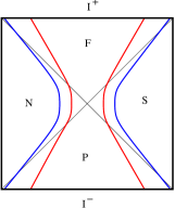
Figure 1: $dS$ future-past extremal surfaces stretching between $I^{\pm}$ on an $S^{d-1}$ equatorial plane. The red curve is for generic subregion while the blue curve is a limiting curve as the subregion becomes the whole space.

Considering the $w=const$ slice as the boundary Euclidean time slice, we consider cap-like subregions defined by $\theta=const$ latitudes on $S^{d-1}$ at $I^{+}$ and equivalent ones at $I^{-}$. Then

$$S=-i{2l^{d-1}V_{S^{d-2}}\over 4G_{d+1}}\int{d\tau\over\tau^{d-1}}(\sin\theta)^{d-2}\sqrt{{1\over 1-\tau^{2}}-(\theta^{\prime})^{2}}$$ (6)

which is difficult to analyse explicitly for caps at generic $\theta$. However at $\theta={\pi\over 2}$ it is straightforward to see that we obtain a future-past extremal surface from the hemispherical cap on $S^{d-1}\in I^{+}$ to the corresponding one at $I^{-}$ [18]. This gives area

$$S=-i{2l^{d-1}V_{S^{d-2}}\over 4G_{d+1}}\int_{\epsilon}^{1}{d\tau\over\tau^{d-1}}{1\over\sqrt{1-\tau^{2}}}\ \ \xrightarrow{\ dS_{4}\ }\ \ -i{\pi l^{2}\over G_{4}}{1\over\epsilon}$$ (7)

with no finite part.

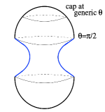
Figure 2: Global $dS$ future-past extremal surfaces stretching between $I^{\pm}$ on any $S^{d}$ equatorial plane in the IR limit ($\theta={\pi\over 2}$). This is also the picture for the $w=const$ slice in the static coordinates.

Global:  Here we have sphere foliations with

$$ds_{d+1}^{2}=-d\tau^{2}+l^{2}\cosh^{2}{\tau\over l}d\Omega_{d}^{2}$$ (8)

and we can take the boundary Euclidean time slice to be any $S^{d}$ equatorial plane (which are all equivalent). Then we obtain the area functional (with factor of $2$ for top+bottom)

$$S=-i{2l^{d-2}V_{S^{d-2}}\over 4G_{d+1}}\int d\tau\ (\cosh\tau)^{d-2}\ (\sin\theta)^{d-2}\sqrt{1-\cosh^{2}\tau\,(\partial_{\tau}\theta)^{2}}$$ (9)

which has structural similarities to the $w=const$ slice above. At $\theta={\pi\over 2}$ it is straightforward to see a future-past extremal surface stretching from $I^{+}$ to $I^{-}$ with area (focussing on $dS_{4}$)

$$S=-i{\pi l^{2}\over G_{4}}\int_{0}^{\tau_{c}/l}d\tau\ \cosh\tau\sim-i{\pi l^{2}\over 2G_{4}}e^{\tau_{c}/l}\sim-i{\pi l^{2}\over 2G_{4}}{l\over T_{c}}\ .$$ (10)

This is an area law divergence type term, with no finite part. The last expression has been obtained by noting that near $I^{+}$ we have $ds^{2}=-d\tau^{2}+l^{2}e^{2\tau/l}d\Omega_{3}^{2}\sim{l^{2}\over T^{2}}(-dT^{2}+l^{2}d\Omega_{3}^{2})$, with cutoff $T_{c}=le^{-\tau_{c}/l}\sim 0$ near $\tau_{c}\rightarrow\infty$. The area law divergence is structurally similar to the static coordinates case earlier.

Poincare:  The full de Sitter space is obtained from two Poincare patches joined at the past horizon $\tau\rightarrow-\infty$. Now based on the above descriptions for the static and global coordinate systems, we can likewise construct future-past surfaces by imposing regularity boundary conditions on the past horizon. For the surface stretching down from $I^{+}$ described by the extremization (2), we require that the derivatives $\partial_{\tau}x$ match smoothly onto the corresponding ones for a corresponding surface stretching up from $I^{-}$. Note that $(\partial_{\tau}x)^{2}\rightarrow 1$ as $\tau\rightarrow-\infty$. The detailed continuation is similar to that in [18, 19] for the static coordinates. This leads to just the area law term again, giving $S_{dS_{4}}\sim-i{2l^{2}\over 4G_{4}}{V\over\epsilon}$ .

2.2 $dS$ no-boundary surfaces

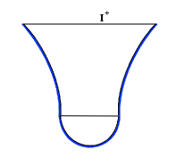
Figure 3: Global $dS$ no-boundary extremal surfaces, with a top timelike part joining smoothly with a spatial part going around the hemisphere in the bottom half. The blue curve is the IR limit ($\theta={\pi\over 2}$) on some $S^{d}$ equatorial plane. This is also the picture for the $w=const$ slice in the static coordinates.

In accord with the Hartle-Hawking no-boundary prescription [31] (see also [32]), let us cut global de Sitter space in the middle, on the $\tau=0$ time slice and join the top half with a hemisphere in the bottom half: this hemisphere is given by the Euclidean continuation

$$ds^{2}=l^{2}d\tau_{E}^{2}+l^{2}\cos^{2}\tau_{E}\,d\Omega_{d}^{2}\,;\qquad\quad\tau=il\tau_{E}\,,\quad 0\leq\tau_{E}\leq{\pi\over 2}\,.$$ (11)

Consider now some $S^{d}$ equatorial plane (i.e. $S^{d-1}$) and the timelike extremal surface in (9), at $\theta={\pi\over 2}$ which is the IR limit of such surfaces. The top part of this surface from $I^{+}$ hits the $\tau=0$ mid-slice “vertically”: we join this smoothly at $\tau=0$ with a surface that goes around the bottom hemisphere, Figure 3 (see [21] for $dS_{3}$)). This joining being smooth implies consistency with the Hartle-Hawking prescription. This IR surface is

$ds^{2}=l^{2}d\tau_{E}^{2}+l^{2}\cos^{2}\tau_{E}(d\theta^{2}+\sin^{2}\theta\,d\Omega_{d-2}^{2}))\Big{|}_{\theta={\pi\over 2}}=l^{2}d\tau_{E}^{2}+l^{2}\cos^{2}\tau_{E}d\Omega_{d-2}^{2}$

and gives area

$${l^{d-1}\over 4G_{d+1}}V_{S^{d-2}}\int_{0}^{\pi/2}d\tau_{E}\ (\cos\tau_{E})^{d-2}\,=\,{l^{d-1}\over 4G_{d+1}}V_{S^{d-2}}\,{\sqrt{\pi}\,\Gamma({d-1\over 2})\over 2\,\Gamma({d\over 2})}\,=\,{1\over 2}{l^{d-1}\,V_{S^{d-1}}\over 4G_{d+1}}\ ,$$ (12)

using the expression $V_{S^{d}}={2\pi^{(d+1)/2}\over\Gamma((d+1)/2)}$ for a $d$-sphere. This real part of the area of this spacelike surface on the hemisphere is precisely half of de Sitter entropy. This recovery of the entropy is in detail somewhat different from the realization of de Sitter entropy as the area of the cosmological horizon from the point of view of static patch observers. In particular, one of the hemisphere directions that enters here is the Euclidean continuation of the time direction in the future universe.

Focussing on $dS_{4}$, the full area for this no-boundary surface is the sum of the top timelike part (which is half of the future-past area (10)) and the hemisphere part becomes

$$S=-i{\pi l^{2}\over 4G_{4}}{l\over T_{c}}+{\pi l^{2}\over 2G_{4}}\ .$$ (13)

There are some similarities between these no-boundary surface areas and the semiclassical Wavefunction $\Psi_{dS}=e^{iS_{cl}}$ for no-boundary $dS_{4}$, with $S_{cl}$ the action. The top Lorentzian half has real $S_{cl}$ which gives a pure phase in $\Psi_{dS}$. The bottom hemisphere arises after the continuation (11) to Euclidean time (the no-boundary point is $\tau_{E}={\pi\over 2}$ here): $iS_{cl}$ continues to the Euclidean gravity action  $-\int_{{}_{{}_{nbp}}}\sqrt{g}\,(R-2\Lambda)$  pertaining to the hemisphere, which for $dS_{4}$ gives ${1\over 2}\,{l^{4}V_{S^{4}}\over 16\pi G_{4}}\,{6\over l^{2}}={\pi l^{2}\over 2G_{4}}$ as is well-known (see e.g. [33, 34]).

A similar calculation of the spatial surface on the hemisphere can be done for the timelike future-past surface in the static coordinates discussed earlier. In this case, the boundary was $R_{w}\times S^{d-1}$ leading to either any $S^{d-1}$ equatorial plane or the $w=const$ slice as the boundary Euclidean time slice. The Euclidean continuation in this case is

$$ds^{2}=l^{2}(\cos^{2}\psi\,d\tau_{E}^{2}+d\psi^{2}+\sin^{2}\psi\,d\Omega_{d-1}^{2})\,,\qquad t=i\tau_{E}\,,\quad r=l\sin\psi\ ,$$ (14)

where $\tau_{E}\in[0,2\pi l]$ and $0\leq\psi\leq{\pi\over 2}$ . First, considering the $S^{d-1}$ equatorial plane surfaces, we saw that there is a limiting surface at $\tau_{*}>1$ (this is $\tau_{*}=\sqrt{2}$ for $dS_{4}$) which translates to some limiting value $\psi_{*}$ given by $\sin\psi_{*}={r_{*}\over l}={1\over\tau_{*}}$ . Then the surface is described by

$$\!ds^{2}=\cos^{2}\psi_{*}d\tau_{E}^{2}+\sin^{2}\psi_{*}d\Omega_{d-2}^{2}\quad\rightarrow\quad Area=\int_{0}^{\pi l}\cos\psi_{*}d\tau_{E}\,(\sin\psi_{*})^{d-2}\,V_{S^{d-2}}\,{l^{d-2}\over 4G_{d+1}}\,.$$ (15)

Focussing on $dS_{4}$ we have $\sin\psi_{*}={1\over\tau_{*}}={1\over\sqrt{2}}$ giving the area ${1\over 2}\,(\pi l)\,{2\pi\,l\over 4G_{4}}={\pi^{2}\,l^{2}\over 4G_{4}}$ . This apparently unrecognizable value is perhaps not surprising due to the limiting surface.

For the $w=const$ slice (equivalently $\tau_{E}=const$), the timelike surface from the $\theta={\pi\over 2}$ cap on $S^{d-1}$ leads on the hemisphere to

$$ds^{2}=d\psi^{2}+\sin\psi^{2}\,d\Omega_{d-2}^{2}\quad\rightarrow\quad Area={l^{d-1}\,V_{S^{d-2}}\over 4G_{d+1}}\int_{0}^{\pi/2}d\psi\,(\sin\psi)^{d-2}={1\over 2}{l^{d-1}\,V_{S^{d-1}}\over 4G_{d+1}}\ ,$$ (16)

identical to global $dS$ (12) above, not surprising given the similarities in the calculation for this slice. With the top timelike part from (7), the total area becomes $S=-i{\pi l^{2}\over 2G_{4}}{1\over\epsilon}+{\pi l^{2}\over 2G_{4}}$ for $dS_{4}$.

Note that all these no-boundary surfaces turn around only in the bottom hemisphere: the top timelike half is identical to the corresponding future-past surface and there is no $I^{+}\rightarrow I^{+}$ turning point there. Thus if we consider two disjoint subregions the corresponding no-boundary surfaces are unique (following from the top halves of the corresponding future-past surfaces), with no new connected surface emerging: so $S[A\cup B]=S[A]+S[B]$. Thus, as for the future-past surfaces [19], mutual information vanishes here as well.

2.3 2-dim CFT, timelike subsystems, complex EE

Now consider $dS_{3}$, special for various reasons. In entirely Lorentzian global de Sitter, the future-past surfaces on some $S^{2}$ equatorial plane slice (9) give area $S=-i{l\over G_{3}}\log{l\over T_{c}}$ . If we consider no-boundary $dS_{3}$, the total area from the top timelike part and the hemisphere part (12) becomes

$$S_{dS_{3}}=-i{l\over 2G_{3}}\log{l\over T_{c}}+{\pi l\over 4G_{3}}$$ (17)

The last (real) term is half $dS_{3}$ entropy ${\pi l\over 2G_{3}}$ . The whole expression can be seen to be an overall $-i$ times the familiar ${c\over 6}\log{L^{2}\over\epsilon^{2}}$ [35, 36, 37] with $c={3l_{AdS}\over 2G}$ the $AdS_{3}$ central charge, alongwith ${l^{2}\over T_{c}^{2}}\rightarrow-{l^{2}\over T_{c}^{2}}$ (so $\log(-1)=i\pi$). Note that $dS_{3}/CFT_{2}$ has $c_{dS_{3}}=-i{3l_{dS}\over 2G}$ [5] which for single intervals would give imaginary $S$ as for the entirely Lorentzian future-past surfaces stated above. So perhaps what is most striking in (17) is the real part arising from the hemisphere which then requires an additional $i$, which is a novel feature of this Euclidean CFT${}_{dS_{3}}$ dual (in contrast with ordinary Euclidean CFTs with simply real spatial lengths and no time). Further related comments appear in sec. 4.

To put this in perspective, for ordinary unitary 2-dim CFTs, the entanglement entropy is

$$S={c\over 6}\log{\Delta^{2}\over\epsilon^{2}}={c\over 6}\log{-(\Delta t)^{2}+(\Delta x)^{2}\over\epsilon^{2}}\ .$$ (18)

For ordinary spacelike intervals $\Delta^{2}$, we obtain the familiar $S={c\over 3}\log{\Delta x\over\epsilon}$ . On the other hand suppose we rotate the subsystem to be entirely timelike with some width $\Delta t$ in the time direction. This gives

$$S={c\over 3}\log{\Delta t\over\epsilon}+{c\over 6}(i\pi)$$ (19)

the imaginary part arising from $\log(-1)$ in the timelike separation in the interval (more generally the real part contains $\Delta^{2}<0$). This imaginary part has appeared previously in studies of quantum extremal surfaces in de Sitter with regard to the future boundary [23, 24]. The bulk matter is modelled as a 2-dim CFT with some central charge $c>0$ but the timelike separation of the quantum extremal surface gives $\Delta^{2}<0$ in (18) above.

The usual replica formulation of entanglement entropy for a single interval proceeds by picking the interval $\Delta x\equiv[u,v]$ on some Euclidean time slice $\tau_{E}=const$, then constructing $n$ replica copies glued at the interval endpoints. Evaluating ${\rm Tr}\rho_{A}^{n}$ can be mapped to the twist operator 2-point function which then leads finally to the entanglement entropy $S_{A}=-\lim_{n\rightarrow 1}\partial_{n}{\rm Tr}\rho_{A}^{n}$. The only data here is the CFT central charge and the interval in question. The above Euclidean formulation applies for a timelike interval as well, with the only change being that the Euclidean time slice is $x=const$ and the interval is $\Delta t\equiv[u_{t},v_{t}]$. However in continuing back to Lorentzian time, we rotate $u_{t},v_{t}$, to $-iu_{t},\ -iv_{t}$, and so we obtain $\Delta^{2}=-(v_{t}-u_{t})^{2}=-(\Delta t)^{2}$, which gives (19) above. This of course requires that the CFT contains some time direction.

It is also worth noting that complex-valued entanglement entropy arises quite explicitly in studies of ghost-like theories and simple quantum mechanical toy models of “ghost-spins” [25, 26]: in this case the reduced density matrix acquires minus signs due to contributions from negative norm states. Defining contractions over the ghost-spin Hilbert space appropriately leads to consistent expressions for the reduced density matrix and entanglement entropy, which are in general complex-valued.

3 “Time-entanglement” in quantum mechanics

We have constructed future-past extremal surfaces stretching from $I^{+}$ to $I^{-}$. Since they are entirely timelike, their area is pure imaginary, with an overall $-i$ relative to the area of the familiar spacelike RT/HRT surfaces in $AdS$. However, apart from this overall $-i$, the area is real and positive: the overall $-i$ is a uniform factor, for any subregion at $I^{+}$. This is a bit reminiscent of the length of timelike geodesics having an overall $-i$ relative to the length of spacelike geodesics. We call this timelike length as “time” rather than “$-i\cdot$space”. This suggests that the areas of the entirely timelike future-past extremal surfaces encode some new object, “time-entanglement”.

Recall now the appearance of complex-valued areas for the no-boundary surfaces which are closely related to the entirely timelike future-past surfaces: they comprise a timelike component which is identical to the top half of the future-past one and a spacelike component from the hemisphere glued in the bottom half. The area is now complex, with a pure imaginary part from the top timelike component and a real part from the hemisphere component.

We now describe two aspects of this notion of “time-entanglement” in quantum mechanics (independent of de Sitter at this point). The first is based on the thermofield-double type state described in [18, 19], while the second is based on the time-evolution operator, regarding the timelike surfaces as some sort of transition amplitude.

3.1 A future-past thermofield double state

The entirely timelike future-past surfaces, akin to rotated Hartman-Maldacena surfaces [20], suggest some sort of entanglement between $I^{\pm}$, so consider

$$|\psi\rangle_{fp}=\sum\psi^{i_{n}^{F},i_{n}^{P}}|i_{n}\rangle_{F}|i_{n}\rangle_{P}\ ,$$ (20)

This was written down in [18] as an entirely positve object entangling identical $F$ and $P$ components (with intuition based on the TFD state for the eternal black hole [30]). A partial trace over the second ($P$) copy gives a reduced density matrix with nontrivial entanglement entropy. To see how this works, let us consider a very simple toy example of a 2-state system in ordinary quantum mechanics. The action of the Hamiltonian $H$ on these (orthogonal basis) eigenstates and the resulting (simple) time evolution are

$$H|k\rangle=E_{k}|k\rangle\,,\quad k=1,2\ ;\qquad\quad|k\rangle_{F}\equiv|k(t)\rangle=e^{-iE_{k}t}|k\rangle_{P}\ .\qquad\quad[\langle 1|2\rangle=0]$$ (21)

We consider the $F$ and $P$ slices to be separated by time $t$ and obtain the $F$ state from the $P$ state by time evolution through $t$. The future-past TFD state (20) in this toy case is

$$|\psi\rangle_{fp}={1\over\sqrt{2}}|1\rangle_{F}|1\rangle_{P}+{1\over\sqrt{2}}|2\rangle_{F}|2\rangle_{P}={1\over\sqrt{2}}e^{-iE_{1}t}|1\rangle_{P}|1\rangle_{P}+{1\over\sqrt{2}}e^{-iE_{2}t}|2\rangle_{P}|2\rangle_{P}\ ,$$ (22)

We have normalized the coefficients for maximal entanglement at $t=0$. For nonzero $t$, there are extra phases due to the time evolution but they cancel in the reduced density matrix obtained by tracing $|\psi\rangle_{fp}\langle\psi|_{fp}$ over the entire second copy as $\delta_{ij}\psi_{fp}^{ki}(\psi_{fp}^{*})^{lj}$, so

$$\rho_{fp}={\rm Tr}_{P}|\psi\rangle_{fp}\langle\psi|_{fp}={1\over 2}|1\rangle_{F}\langle 1|_{F}+{1\over 2}|2\rangle_{F}\langle 2|_{F}\ .$$ (23)

Now imagine a 2-spin analogy, with $|1\rangle=|++\rangle$, $|2\rangle=|--\rangle$, i.e. we identify $1\rangle,|2\rangle$ with the 2-state subspace $|\pm\pm\rangle$ of two spins with states $|\pm\rangle$ each for simplicity and concreteness. Then a partial trace over the second component gives the reduced density matrix $Tr_{2}\rho_{fp}={1\over 2}|+\rangle_{F}\langle+|_{F}+{1\over 2}|-\rangle_{F}\langle-|_{F}$ again with an entirely positive structure, and entropy $\log 2$.

If the states in question are not ordinary spins but “ghost-spins” with negative norm states, as discussed in [18] based on the studies in [25, 26], the fact that we have entangled identical components in both the future and past copies ensures that the minus signs cancel in $\gamma_{\sigma\rho}\psi_{fp}^{\alpha\sigma}(\psi_{fp}^{*})^{\beta\rho}$ (with $\gamma_{ij}$ the indefinite ghost-spin metric) again yielding an entirely positive structure.

This future-past TFD state with timelike separation is quite different in principle from the usual TFD state. This positive structure despite the timelike separation is in some sense similar in spirit to the areas of the entirely timelike surfaces after stripping off the universal overall $-i$.

3.2 Time-evolution and reduced transition amplitudes

Unlike $AdS$ where specifying boundary data fixes the extremization problem, $dS$ extremal surfaces starting at late times on $I^{+}$ do not return, thus requiring extra data on boundary conditions in the far past. This is reminiscent of scattering amplitudes, i.e. final states from initial states, or equivalently time evolution. It is then amusing to ask for entanglement-like structures arising from the time evolution operator ${\cal U}(t)$ after a partial trace over some environment: in other words, we look for a “reduced transition amplitude” and its entropy. This suggests (taking $A$ subregion, $B$ environment)

$$\rho_{t}(t)\equiv{{\cal U}(t)\over{\rm Tr}\,{\cal U}(0)}\quad\rightarrow\quad\rho_{t}^{A}=tr_{B}\,\rho_{t}\quad\rightarrow\quad S_{A}=-tr(\rho_{t}^{A}\log\rho_{t}^{A})\ .$$ (24)

The normalization is so we obtain ordinary entanglement structures at $t=0$, as we will see explicitly. To illustrate, consider again the very simple toy example (21) above. Since everything is diagonal here, the normalized time evolution operator is simple, becoming

$${\cal U}(t)=e^{-iHt}:\qquad\rho_{t}(t)={1\over 2}e^{-iE_{1}t}|1\rangle_{P}\langle 1|_{P}+{1\over 2}e^{-iE_{2}t}|2\rangle_{P}\langle 2|_{P}={1\over 2}|1\rangle_{F}\langle 1|_{P}+{1\over 2}|2\rangle_{F}\langle 2|_{P}\ .$$ (25)

Now recall the 2-spin analogy: $|1\rangle=|++\rangle$,  $|2\rangle=|--\rangle$. A partial trace over the second components gives

$$\rho_{t}^{A}={1\over 2}e^{-iE_{1}t}|+\rangle_{P}\langle+|_{P}+{1\over 2}e^{-iE_{2}t}|-\rangle_{P}\langle-|_{P}\ ,$$ (26)

$$S_{A}=-\sum_{i}{1\over 2}e^{-iE_{i}t}\log\Big{(}{1\over 2}e^{-iE_{i}t}\Big{)}={1\over 2}\log 2(e^{-iE_{1}t}+e^{-iE_{2}t})+{1\over 2}(iE_{1}t)e^{-iE_{1}t}+{1\over 2}(iE_{2}t)e^{-iE_{2}t}.$$ (27)

Normalizing ${\cal U}(t)$ by its trace at time $t$ gives ${\rm Tr}\rho_{t}(t)=1$ for all $t$ (not just $t=0$), modifying (24)-(27) to

$$\rho_{t}(t)\equiv{{\cal U}(t)\over{\rm Tr}\,{\cal U}(t)}\quad \Rightarrow \quad\rho_{t}(t)=\sum_{i}p_{i}\,|i\rangle_{P}\langle i|_{P}\ ,\qquad p_{i}={e^{-iE_{i}t}\over\sum_{j}e^{-iE_{j}t}}\ ,$$

$$\rightarrow\ \ \ \rho_{t}^{A}=\sum_{i}p_{i}^{\prime}\,|i^{\prime}\rangle_{P}\langle i^{\prime}|_{P}\quad \rightarrow \quad S_{A}=-\sum_{i}p_{i}^{\prime}\,\log p_{i}^{\prime}\ ,$$ (28)

where $H|i\rangle=E_{i}|i\rangle$ and the second line arises after partial trace. There are similarities with pseudo-entropy [38] although the details above look different a priori. There are close interrelations between time entanglement above (entanglement-like structures based on the time evolution operator regarded as a density operator) and pseudo-entropy: some of these explorations in quantum mechanics with various interesting new features appear in [39], which also elaborates on some results outlined below.

$\rho_{t}^{A}$ resembles an ordinary maximally entangled state at $t=0$. Any later time $t\neq 0$ gives complex-valued entropy in general (although there are real subfamilies: e.g. (3.2) for the 2-state case contains a single phase $e^{-i(E_{2}-E_{1})t}$ and gives $S_{A}$ real). Further the different normalizations give different results in detail, as is already clear in the simple cases above. Overall these structures resemble the usual finite temperature mixed state entanglement, except with imaginary temperature, i.e. $\beta=it$.

There are also related quantities that arise along similar lines. For instance the time evolution operator ${\cal U}(t)$ alongwith a projection operator onto a generic state $|I\rangle$ gives  ${\cal U}(t)|I\rangle\langle I|=|F_{I}(t)\rangle\langle I|$ where $|F_{I}(t)\rangle$ is the future state time-evolved from the initial state $|I\rangle$. Normalizing at time $t$ and performing a partial trace gives a reduced transition matrix which resembles that in pseudo-entropy [38] but with the future state specifically corresponding to the time evolved state. Relatedly, normalizing at $t=0$ gives different structures. For instance, projection onto Hamiltonian eigenstates $|E_{I}\rangle$ and performing partial trace gives simple phases for $\rho_{t}^{A,I}$ (essentially components of (26)), so the corresponding entropy (27) is of the form e.g. $iE_{I}t\,e^{-iE_{I}t}$.

4 Discussion: $dS$ surfaces, time contours, rotations

We have seen that the absence of $I^{+}\rightarrow I^{+}$ turning points for $dS$ extremal surfaces anchored at the future boundary leads to either future-past surfaces or no-boundary surfaces. Since these surfaces are characterized by area integrals which ultimately reduce to simple integrals over the time direction, they can be organized and recast in terms of time contours, which leads to certain clarifications. Towards this, recall that the future-past and no-boundary surface areas (9), (12), are of the schematic form (with a reduced area functional $a(\tau)$)

$$S_{fp}\sim 2\cdot-iS_{0}\int_{\tau_{{}_{cF}}}^{\tau_{*}}d\tau\,a(\tau)\,,\qquad\qquad [\tau:\tau_{{}_{cF}}\rightarrow\tau_{*}\rightarrow\tau_{{}_{cP}}]\,;$$

$$S_{nb}\sim-iS_{0}\int_{\tau_{{}_{cF}}}^{\tau_{*}}d\tau\,a(\tau)+S_{0}\int_{\tau_{E*}}^{nbp}d\tau_{E}\,a_{E}(\tau_{E})\,,\quad [\tau:\tau_{{}_{cF}}\rightarrow\tau_{*}\rightarrow nbp]\,,$$ (29)

where $S_{0}$ is de Sitter entropy, $\tau_{cF}$ labels the anchoring cutoff slice at $I^{+}$ and $\tau_{*}$ is the bulk point where the surface is going “vertically down” (Figures 2, 3). $nbp$ refers to the no-boundary point. In the no-boundary surfaces, the time contour goes along the real time direction till $\tau_{*}$ and then along the Euclidean time path till the $nbp$. As we saw, these simplify in the IR limit to give

$$S_{fp}=-2iS_{0}\,I[\tau_{{}_{cF}},\tau_{*}]\,;\qquad S_{nb}=-iS_{0}\,I[\tau_{{}_{cF}},\tau_{*}]+{S_{0}\over 2}\,;$$

$$\qquad\qquad\quad\Rightarrow\qquad S_{fp}=S_{nb}-S_{nb}^{*}\ .$$ (30)

In this light, it is reasonable to think that the future-past surface is made of two copies of the no-boundary surface, but with the time contour schematically being $[\tau_{{}_{cF}}\rightarrow\tau_{*}\rightarrow\tau_{{}_{cP}}]=[\tau_{{}_{cF}}\rightarrow\tau_{*}\rightarrow nbp]+[nbp\rightarrow\tau_{*}\rightarrow\tau_{{}_{cP}}]$. Then the real parts in the two copies of $S_{nb}$ cancel to give a pure imaginary $S_{fp}$. Regarding $S_{nb}$ as some time entanglement entropy arising from one dual boundary Euclidean CFT copy $Z_{CFT}=\Psi_{dS}$ via $dS/CFT$ [3, 4, 5] suggests regarding $S_{fp}$ as arising from two copies $\Psi_{dS}^{*}\Psi_{dS}$. It would be interesting to flesh this out more precisely from a replica formulation, perhaps developing [40] here.

Looking now at the expressions in detail for $dS_{3}$ and $dS_{4}$, i.e. (17), (10), (13), we have

$$dS_{3}: \quad S_{fp}=-i\,{l\over G_{3}}\log{l\over\epsilon}\,;\qquad S_{nb}=-i\,{l\over 2G_{3}}\log{l\over\epsilon}+{l\over 2G_{3}}\,{\pi\over 2}\,.$$

$$dS_{4}: \quad S_{fp}=-i\,{\pi l^{2}\over 2G_{4}}{l\over\epsilon}\,;\qquad\ \ S_{nb}=-i\,{\pi l^{2}\over 4G_{4}}{l\over\epsilon}+{\pi l^{2}\over 2G_{4}}\,,$$ (31)

with $\epsilon\equiv T_{c}$ in the $dS_{4}$ expressions (10), (13). For $dS_{5}$ there are pure imaginary subleading divergent terms as well, from the timelike $I$ integral in (4). Writing the $dS_{3}$ expression as

$$dS_{3}:\quad S_{nb}=-i\,\Big{(}{c\over 3}\log{l\over\epsilon}+{c\over 6}\,(i\pi)\,\Big{)}\,,\qquad\quad c={3l\over 2G_{3}}\,,$$ (32)

suggests that these no-boundary surfaces are a rotation from some surfaces in $AdS_{3}$, with central charge $c_{AdS_{3}}=c$  (recall that the $dS_{3}/CFT_{2}$ central charge is $c_{dS_{3}}=-ic$): specifically the overall $-i$ arises from the $AdS_{3}$ radial integral reinterpreted as a time integral in $dS_{3}$. The term inside the brackets is essentially the entanglement entropy (19) for a timelike interval in 2-dim CFT: the real logarithmic part is a spatial area contribution in $AdS_{3}$, while the imaginary part is a timelike contribution). Thus the real spacelike part of the $dS_{3}$ surface, from the Euclidean hemisphere, maps to a pure imaginary, timelike, contribution in $AdS_{3}$.

The $dS_{4}$ case (13) can be similarly recast as

$$dS_{4}:\quad S_{nb}=-i\,\Big{(}{\pi l^{2}\over 4G_{4}}{l\over\epsilon}+i\,{\pi l^{2}\over 2G_{4}}\Big{)}\,,\qquad S_{0}={\pi l^{2}\over G_{4}}\ ,$$ (33)

which again resembles an overall rotation from an $AdS_{4}$ surface, encoded by the overall $-i$. Again, the term inside has a real part corresponding to half of the Hartman-Maldacena-like spacelike surface contribution while the imaginary part is a timelike contribution. The fact that all de Sitter no-boundary surfaces have area of the form (4), i.e.

$$S_{nb}=-i\,\Big{(}S_{0}\,I+i\,{S_{0}\over 2}\Big{)}\,,$$ (34)

suggests that the surfaces can be regarded as space-time rotations from timelike subregions in $AdS$-like spaces. In general these are distinct from analytic continuations of Poincare $AdS$ RT expressions, which correspond to distinct time contours (along imaginary time paths) [14, 15, 16]: e.g. in $dS_{4}$ those give real negative area. However these can be mapped to other appropriate analytic continuations from $AdS$ (see [29]).

Note that this is consistent with the $dS$ future-past surfaces (see Figure 1) being akin to space-time rotations of Hartman-Maldacena surfaces in the $AdS$ black hole [20], as discussed in [18, 19]. In that case, the $dS$ area $S_{fp}$ is pure imaginary, with the overall $-i$ encoding the rotation from a real spacelike area in $AdS$.

The pure imaginary part of the no-boundary $dS_{3}$ surface area can be identified with ${c\over 3}\log{l\over\epsilon}$ for a half-size interval in a Euclidean CFT on a circle [36]: the future-past surfaces have twice this area, and so correspond to two copies. The real spacelike part of the no-boundary area, arising from a deep interior Euclideanization of de Sitter, presumably indicates some new IR aspect of the dual Euclidean CFT that encodes “interior regularity”.

There are some parallels in the thinking in sec. 3 via the time evolution operator and viewing de Sitter space as a collection of past-future amplitudes [4]. This suggests using the S-matrix $|f\rangle\langle i|$ with initial and final states appropriate to $dS$ to analyse entanglement-like structures. Needless to say, there are many things to explore here, in quantum mechanics, de Sitter holography and time.

Acknowledgements:  It is a pleasure to thank Abhijit Gadde, Alok Laddha, Shiraz Minwalla and Sandip Trivedi for helpful discussions. I also thank Tadashi Takayanagi for conversations on the overall $-i$ following [18], which have influenced my thinking. This work is partially supported by a grant to CMI from the Infosys Foundation.

References

- [1]
- [2] M. Spradlin, A. Strominger and A. Volovich, “Les Houches lectures on de Sitter space,” hep-th/0110007.
- [3] A. Strominger, “The dS / CFT correspondence,” JHEP 0110, 034 (2001) [hep-th/0106113].
- [4] E. Witten, “Quantum gravity in de Sitter space,” [hep-th/0106109].
- [5] J. M. Maldacena, “Non-Gaussian features of primordial fluctuations in single field inflationary models,” JHEP 0305, 013 (2003), [astro-ph/0210603].
- [6] D. Anninos, T. Hartman and A. Strominger, “Higher Spin Realization of the dS/CFT Correspondence,” Class. Quant. Grav. 34, no. 1, 015009 (2017) doi:10.1088/1361-6382/34/1/015009 [arXiv:1108.5735 [hep-th]].
- [7] J. M. Maldacena, “The large N limit of superconformal field theories and supergravity,” Adv. Theor. Math. Phys. 2, 231 (1998) [Int. J. Theor. Phys. 38, 1113 (1999)] [arXiv:hep-th/9711200].
- [8] S. S. Gubser, I. R. Klebanov and A. M. Polyakov, “Gauge theory correlators from non-critical string theory,” Phys. Lett. B 428, 105 (1998) [arXiv:hep-th/9802109].
- [9] E. Witten, “Anti-de Sitter space and holography,” Adv. Theor. Math. Phys. 2, 253 (1998) [arXiv:hep-th/9802150].
- [10] G. W. Gibbons and S. W. Hawking, “Cosmological Event Horizons, Thermodynamics, and Particle Creation,” Phys. Rev. D 15, 2738 (1977). doi:10.1103/PhysRevD.15.2738
- [11] S. Ryu and T. Takayanagi, “Holographic derivation of entanglement entropy from AdS/CFT,” Phys. Rev. Lett. 96, 181602 (2006) [hep-th/0603001].
- [12] S. Ryu and T. Takayanagi, “Aspects of Holographic Entanglement Entropy,” JHEP 0608, 045 (2006) [hep-th/0605073].
- [13] V. E. Hubeny, M. Rangamani and T. Takayanagi, “A Covariant holographic entanglement entropy proposal,” JHEP 0707 (2007) 062 [arXiv:0705.0016 [hep-th]].
- [14] K. Narayan, “de Sitter extremal surfaces,” Phys. Rev. D 91, no. 12, 126011 (2015) [arXiv:1501.03019 [hep-th]].
- [15] K. Narayan, “de Sitter space and extremal surfaces for spheres,” Phys. Lett. B 753, 308 (2016) [arXiv:1504.07430 [hep-th]].
- [16] Y. Sato, “Comments on Entanglement Entropy in the dS/CFT Correspondence,” Phys. Rev. D 91, no. 8, 086009 (2015) [arXiv:1501.04903 [hep-th]].
- [17] M. Miyaji and T. Takayanagi, “Surface/State Correspondence as a Generalized Holography,” PTEP 2015, no. 7, 073B03 (2015) doi:10.1093/ptep/ptv089 [arXiv:1503.03542 [hep-th]].
- [18] K. Narayan, “On extremal surfaces and de Sitter entropy,” Phys. Lett. B 779, 214 (2018) [arXiv:1711.01107 [hep-th]].
- [19] K. Narayan, “de Sitter future-past extremal surfaces and the entanglement wedge,” Phys. Rev. D 101, no.8, 086014 (2020) doi:10.1103/PhysRevD.101.086014 [arXiv:2002.11950 [hep-th]].
- [20] T. Hartman and J. Maldacena, “Time Evolution of Entanglement Entropy from Black Hole Interiors,” JHEP 1305, 014 (2013) [arXiv:1303.1080 [hep-th]].
- [21] Y. Hikida, T. Nishioka, T. Takayanagi and Y. Taki, “CFT duals of three-dimensional de Sitter gravity,” JHEP 05, 129 (2022) doi:10.1007/JHEP05(2022)129 [arXiv:2203.02852 [hep-th]].
- [22] Y. Hikida, T. Nishioka, T. Takayanagi and Y. Taki, “Holography in de Sitter Space via Chern-Simons Gauge Theory,” Phys. Rev. Lett. 129, no.4, 041601 (2022) [arXiv:2110.03197 [hep-th]].
- [23] Y. Chen, V. Gorbenko and J. Maldacena, “Bra-ket wormholes in gravitationally prepared states,” JHEP 02, 009 (2021) doi:10.1007/JHEP02(2021)009 [arXiv:2007.16091 [hep-th]].
- [24] K. Goswami, K. Narayan and H. K. Saini, “Cosmologies, singularities and quantum extremal surfaces,” JHEP 03, 201 (2022) doi:10.1007/JHEP03(2022)201 [arXiv:2111.14906 [hep-th]].
- [25] K. Narayan, “On extremal surfaces and entanglement entropy in some ghost CFTs,” Phys. Rev. D 94, no. 4, 046001 (2016) [arXiv:1602.06505 [hep-th]].
- [26] D. P. Jatkar and K. Narayan, “Ghost-spin chains, entanglement and -ghost CFTs,” Phys. Rev. D 96, no. 10, 106015 (2017) [arXiv:1706.06828 [hep-th]].
- [27] C. Arias, F. Diaz and P. Sundell, “De Sitter Space and Entanglement,” Class. Quant. Grav. 37, no. 1, 015009 (2020) doi:10.1088/1361-6382/ab5b78 [arXiv:1901.04554 [hep-th]].
- [28] C. Arias, F. Diaz, R. Olea and P. Sundell, “Liouville description of conical defects in dS4, Gibbons-Hawking entropy as modular entropy, and dS3 holography,” JHEP 04, 124 (2020) doi:10.1007/JHEP04(2020)124 [arXiv:1906.05310 [hep-th]].
- [29] K. Doi, J. Harper, A. Mollabashi, T. Takayanagi and Y. Taki, “Pseudo Entropy in dS/CFT and Time-like Entanglement Entropy,” [arXiv:2210.09457 [hep-th]].
- [30] J. M. Maldacena, “Eternal black holes in anti-de Sitter,” JHEP 0304, 021 (2003) [hep-th/0106112].
- [31] J. B. Hartle and S. W. Hawking, “Wave Function of the Universe,” Phys. Rev. D 28, 2960-2975 (1983) doi:10.1103/PhysRevD.28.2960
- [32] J. Maldacena, G. J. Turiaci and Z. Yang, “Two dimensional Nearly de Sitter gravity,” JHEP 01, 139 (2021) doi:10.1007/JHEP01(2021)139 [arXiv:1904.01911 [hep-th]].
- [33] R. Bousso and S. W. Hawking, “The Probability for primordial black holes,” Phys. Rev. D 52, 5659-5664 (1995) doi:10.1103/PhysRevD.52.5659 [arXiv:gr-qc/9506047 [gr-qc]].
- [34] R. Bousso and S. W. Hawking, “Pair creation of black holes during inflation,” Phys. Rev. D 54, 6312-6322 (1996) doi:10.1103/PhysRevD.54.6312 [arXiv:gr-qc/9606052 [gr-qc]].
- [35] C. Holzhey, F. Larsen and F. Wilczek, “Geometric and renormalized entropy in conformal field theory,” Nucl. Phys. B 424, 443 (1994) [hep-th/9403108].
- [36] P. Calabrese and J. L. Cardy, “Entanglement entropy and quantum field theory,” J. Stat. Mech. 0406, P06002 (2004) [hep-th/0405152].
- [37] P. Calabrese and J. Cardy, “Entanglement entropy and conformal field theory,” J. Phys. A 42, 504005 (2009) doi:10.1088/1751-8113/42/50/504005 [arXiv:0905.4013 [cond-mat.stat-mech]].
- [38] Y. Nakata, T. Takayanagi, Y. Taki, K. Tamaoka and Z. Wei, “New holographic generalization of entanglement entropy,” Phys. Rev. D 103, no.2, 026005 (2021) [arXiv:2005.13801 [hep-th]].
- [39] K. Narayan and Hitesh K. Saini, “Notes on time entanglement and pseudo-entropy,” [arXiv:2303.01307 [hep-th]].
- [40] A. Lewkowycz and J. Maldacena, “Generalized gravitational entropy,” JHEP 08, 090 (2013) doi:10.1007/JHEP08(2013)090 [arXiv:1304.4926 [hep-th]].