Multi-Agent Path Finding via Tree LSTM

Abstract

In recent years, Multi-Agent Path Finding (MAPF) has attracted attention from the fields of both Operations Research (OR) and Reinforcement Learning (RL). However, in the 2021 Flatland3 Challenge, a competition on MAPF, the best RL method scored only 27.9, far less than the best OR method. This paper proposes a new RL solution to Flatland3 Challenge, which scores 125.3, several times higher than the best RL solution before. We creatively apply a novel network architecture, TreeLSTM, to MAPF in our solution. Together with several other RL techniques, including reward shaping, multiple-phase training, and centralized control, our solution is comparable to the top 2-3 OR methods.

1 Introduction

Multi-agent path finding (MAPF), i.e., finding collision-free paths for multiple agents on a graph, has been a long-standing combinatorial problem. On undirected graphs, a feasible solution can be found in polynomial time, but finding the fastest solution is NP-hard. And on directed graphs, even finding a feasible solution is NP-hard in general cases (Nebel 2020). Despite the great challenges of MAPF, it is of great social and economic value because many real-life scheduling and planning problems can be formulated as MAPF questions. Many operations research (OR) algorithms are proposed to efficiently find sub-optimal solutions (Cohen et al. 2019; Švancara et al. 2019; Ma et al. 2018; Ma, Kumar, and Koenig 2017).

As an important branch in decision theory, reinforcement learning has attracted a lot of attention these years due to its super-human performance in many complex games, such as AlphaGo (Silver et al. 2017), AlphaStar (Vinyals et al. 2019), and OpenAI Five (Berner et al. 2019). Inspired by the tremendous successes of RL on these complex games and decision scenarios, multi-agent reinforcement learning (MARL) is widely expected to work on MAPF problems as well. We study MARL in MAPF problems and aim to provide high-performance and scalable RL solutions. To develop and test our RL solution, we focus on a specific MAPF environment, Flatland.

Flatland (Mohanty et al. 2020; Laurent et al. 2021) is a train schedule simulator developed by the Swiss Federal Railway Company (SBB). It simulates trains and rail networks in the real world and serves as an excellent environment for testing different MAPF algorithms. Since 2019, SBB has successfully held three flatland challenges, attracting more than 200 teams worldwide, receiving thousands of submissions and over one million views. The key reasons why we focus on this environment are as follows,

• Support Massive Agents: On the maximum size of the map, up to hundreds of trains need to be planned.

• Directed Graphs and Conflicts between Agents: Trains CANNOT move back, and all decisions are not revocable. Deadlock occurs if the trains are not well planned (Figure 5), which makes this question very challenging.

• Lack of High-Performance RL Solutions: Existing RL solutions show a significant disadvantage compared with OR algorithms (27.9 vs. 141.0 scores).

To solve Flatland, we propose an RL solution by standard reinforcement learning algorithms at scale. The critical components of our RL solution are (1) the application of a TreeLSTM network architecture to process the tree-structured local observations of each agent, (2) the centralized control method to promote cooperation between agents, and (3) our optimized 20x faster feature parser.

Our contributions can be summarized as (1) We propose an RL solution consisting of domain-specific feature extraction and curriculum training phases design, a TreeLSTM network to process the structured observations, and a 20x faster feature parser to improve the sample efficiency. (2) Our observed strategies and performance show the potential of RL algorithms in MAPF problems. We find that standard RL methods coupled with domain-specific engineering can achieve comparable performance with OR algorithm ($2^{nd}$– $3^{rd}$ OR ). Our solution provides implementation insights to the MARL in the MAPF research community. (3) We open-sourcedour solution and the optimized feature parser for further research on multi-agent reinforcement learning in MAPF problems.

2 Flatland3 Environment

Flatland is a simplified world of rail networks in which stations are connected by rails. Players control trains to run from one station to another. Its newest version, Flatland3, consists of the following rules.

• The time is discretized into timestamps from 0 to ${T_{\mathrm{max}}}$.

• There are $N$ trains and several cities. Trains are numbered from $1$ to $N$.

• Trains’ action space consists of five actions, {do_nothing, forward, stop, left, right}. Trains are not allowed to move backward and must go along the rails.

• Trains have different speeds. Each train $i$ has its own speed $s_{i}$, and can move one step every ${1}/{s_{i}}$ turns. The time cost of one step ${1}/{s_{i}}$ is guaranteed to be an integer, and the largest possible speed is 1, i.e., one step a turn.

• For each train $i$, it has an earliest departure time $A_{i}$ and a latest arrival time $B_{i}$. Each train can depart from its initial station only after its earliest departure time $A_{i}$ and should try its best to arrive at its target station before the latest arrival time $B_{i}$.

• Trains randomly break down (malfunction) while running or waiting for departure. After the breakdown, the train must stay still for a period of time before moving again.

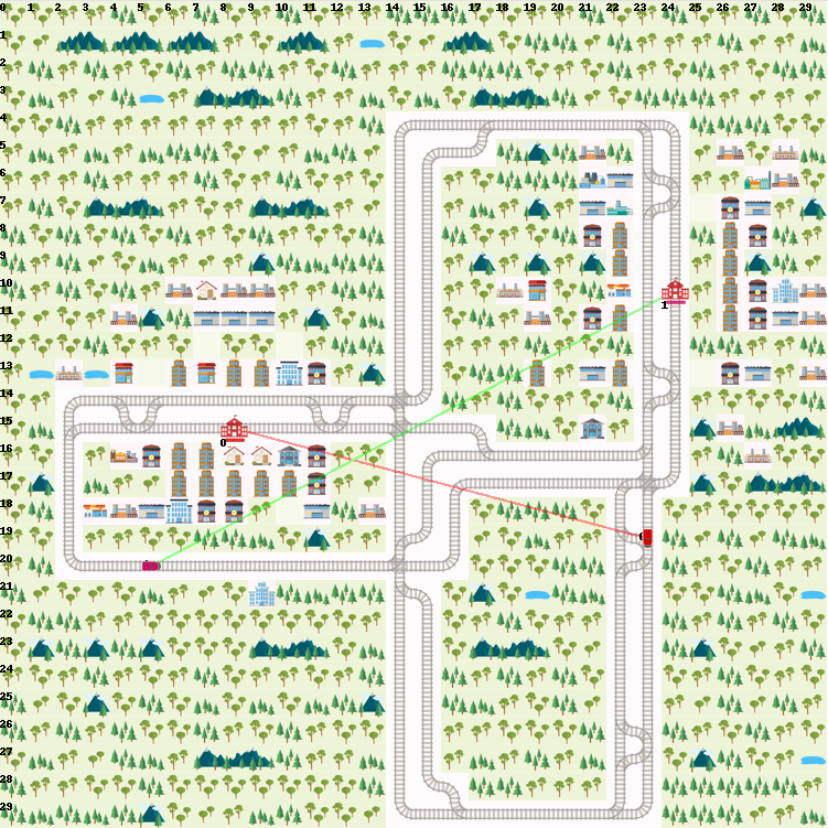
Figure 1: A $30\times 30$ flatland map. There are two stations and two trains. The lines connecting trains and stations indicate trains’ targets.

Figure 2: Different types of rail cells.

Reward

The goal is to control all trains to reach target stations before their latest arrival time $B_{i}$. Every train will get a reward $R_{i}$ in the end. $T_{i}$ denotes the arrival time of each train.

• If a train arrives on time, then it scores 0.

• If it arrives late, it gets a negative reward $B_{i}-T_{i}$ as a penalty, according to how late it is.

• If a train does not manage to arrive at its target before the end time ${T_{\mathrm{max}}}$, then the penalty consists of two parts, a temporal penalty and a spatial penalty. The temporal penalty is $B_{i}-{T_{\mathrm{max}}}$, reflecting how late it is. The spatial penalty is decided by the shortest path distance $d_{i}$ between its final location at time ${T_{\mathrm{max}}}$ and its target.

Formally, $R_{i}$ is defined as

$$R_{i}=\left\{\begin{aligned} &0,&&\text{if}~{}T_{i}\leq B_{i};\\ &B_{i}-T_{i},&&\text{if}~{}B_{i}<T_{i}\leq{T_{\mathrm{max}}};\\ &B_{i}-{T_{\mathrm{max}}}-d_{i}^{({T_{\mathrm{max}}})},&&\text{if}~{}T_{i}>{T_{\mathrm{max}}};\end{aligned}\right.$$ (1)

where $d_{i}^{({T_{\mathrm{max}}})}$ is the distance between train $i$ and its target at time ${T_{\mathrm{max}}}$,

$$d_{i}^{(t)}=d\left((x_{i}^{(t)},y_{i}^{(t)}),\;{\mathrm{target}}_{i}\right).$$ (2)

Our goal is to maximize the sum of individual rewards

$$R=\sum_{i=0}^{N}R_{i}.$$ (3)

Apparently, $R$ is always non-positive, and $R=0$ if and only if all trains reach targets on time. $\lvert R\lvert$ can be arbitrarily large, as long as the map size is sufficiently large and the algorithm performance is sufficiently bad.

Normalized Reward

The magnitude of total reward $R$ greatly relies on the problem scale, such as the number of trains, the number of cities, the speeds of trains, and map size. To make rewards of different problem scales comparable, they are normalized as follows:

$$\bar{R}=1+\frac{R}{N{T_{\mathrm{max}}}},$$ (4)

where $N$ is the number of trains. The environment generating procedure guarantees $\bar{R}\in[0,1]$ by adjusting ${T_{\mathrm{max}}}$. Normalized reward serves as the standard criterion for testing algorithms.

3 Our Approach

The RL solution we provide is cooperative multi-agent reinforcement learning. Each agent independently observes a part of the map localized around itself and encodes the part of the map topology into tree-structured features. Neural Networks independently process each agent’s observation in the first several layers by TreeLSTM, then followed by several self-attention blocks to encourage communications between agents so that a train is able to be aware of others’ local observations and forms its own knowledge of the global map. Rewards are shared by all agents to promote cooperation between them. Our network is trained by Proximal Policy Optimization (PPO) (Schulman et al. 2017) algorithm.

3.1 Feature Extraction

The extracted features consist of two parts, $X^{\mathrm{attr}}$ and $X^{\mathrm{tree}}$.

Agent Attributes

The first part, $X^{\mathrm{attr}}=\{\mathbf{x}^{\mathrm{attr}}_{i}\}_{i=1}^{N}$, are attributes of each agent, such as ID, earliest departure time, latest arrival time, their current state, direction, and the time left, etc. See Table 1 for detailed contents of $X^{\mathrm{attr}}$.

	Name	Dim.	Type
Timetable	Train ID	1	int
	Earliest departure time	1	int
	Latest arrival time	1	int
	Initial direction	4	one-hot
	Initial distance to target	1	int
Spatial	Road type	11	one-hot
	Possible transitions	16	binary
	Current direction	4	one-hot
	Last-turn direction	4	one-hot
	Deadlocked or not	1	binary
	Valid actions	5	binary
	Distance to target	1	int
Temporal	Current time	1	int
	#turns before late	1	int
	Arrival time	1	int
State	State	7	one-hot
	Is off-map state	1	binary
	Is on-map state	1	binary
	Is malfunction state	1	binary
	Is moving or not	1	binary
	Malfunction ends	1	binary
	Left malfunctional turns	1	int
	Speed state-machine	5	int

Table 1: Extracted agent attributes in $X^{\mathrm{attr}}$.

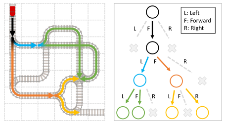
Figure 3: Construct a spanning tree for each agent to encode its possible future paths. Each node represents a branch the agent may choose.

Description	Dim.	Type
#agents in same direction	1	int
#agents in opposite direction	1	int
#agents ready to depart	1	int
#agents in malfunction	1	int
Distance to agent’s own target	1	int
Distance to other agents’ targets, if any	1	int
Distance to other agents, if any	1	int
Distance to potential conflict, if any	1	int
Distance to unusable switch, if any	1	int
Branch length	1	int
Slowest speed of observed agents	1	float

Table 2: Useful information extracted for each node in spanning tree.

Tree Representation of Possible Future Paths

The second part $X^{\mathrm{tree}}$ is the main part of the observations. It encodes possible future paths of each agent as well as useful information about these paths into a tree-like structure. We take the rail network as a directed graph and construct a spanning tree for each agent by a depth-limited BFS (breadth-first-search) starting from its current location. Each node in the tree represents a branch the agent may choose, see Figure 3. Formally, the spanning tree we construct for each train $i$ is $\mathcal{T}_{i}=(\mathcal{V}_{i},\mathcal{E}_{i})$ with node set $\mathcal{V}_{i}$ and edge set $\mathcal{E}_{i}$. Each node $\nu\in\mathcal{V}_{i}$ is associated with a vector $\boldsymbol{x}_{\nu}$, containing useful information about this branch. See Table 2 for detailed contents of $\boldsymbol{x}_{\nu}$. So, $X^{\mathrm{tree}}$ contains both the tree structure and these associated node features:

$$X^{\mathrm{tree}}=\{(\mathcal{T}_{i},X^{\mathrm{tree}}_{i})\}_{i=1}^{N},$$ (5)

where $X^{\mathrm{tree}}_{i}=\{\boldsymbol{x}_{\nu}|\nu\in\mathcal{V}_{i}\}$.

Such tree representation is provided by Flatland3 environment and has also been explored by other RL methods (Mohanty et al. 2020; Laurent et al. 2021). However, no RL method before has achieved comparable performance as ours because we made the following improvements.

• First, all methods before concatenate node features together into a long vector so that it can be fed into MLPs. Normal networks can only process vectors, not tree-like input. After concatenation, the underlying structures of trees are lost. In contrast, we think the tree structures are super important for decision-making and must be preserved, as they encode map topology. In section 3.2, we processing such tree-structured data by a special neural network structure, TreeLSTM (Tai, Socher, and Manning 2015).

• Second, our trees are much deeper than others. Tree depth decides the range of agents’ field of view and thus significantly affects the performance. Extracting tree representation is a computationally intensive task. The flatland3 built-in implementation of tree representation is super slow because of the poor efficiency of Python language and the unnecessary complete ternary tree it uses, so the RL methods before have a very limited tree depth, typically 3. We re-implement tree construction by C++ and prune complete ternary trees into normal trees. Our implementation is 20x faster than the built-in one and enables us to build trees with depths of more than 10.

• Third, we build trees in the BFS manner, while the built-in implementation is in the DFS manner. Constructing a spanning tree in a DFS manner makes some nodes near the root on the graph become far from the root, which is a disadvantage.

3.2 Neural Network Architecture

As shown in Figure 4, our neural networks first process $X^{\mathrm{attr}}$ by a 4-layer MLP and process $X^{\mathrm{tree}}$ by TreeLSTM (Tai, Socher, and Manning 2015). TreeLSTM is a variant of LSTM designed for tree-structured data, whose details will be elaborated later.

$$H^{\mathrm{attr}} =\operatorname{MLP}(X^{\mathrm{attr}})$$ (6)

$$H^{\mathrm{tree}} =\operatorname{TreeLSTM}(X^{\mathrm{tree}})$$ (7)

Then, we concatenate $H^{\mathrm{attr}}$ and $H^{\mathrm{tree}}$ together and feed them into three consecutive self-attention blocks to encourage communications between agents. With the self-attention mechanism (Vaswani et al. 2017), a train is able to be aware of other trains’ observations and forms its own knowledge of the global map.

$$H^{(0)} =[H^{\mathrm{attr}},H^{\mathrm{tree}}],$$ (8)

$$H^{(l)} =\operatorname{Self-Attention}\left(H^{(l-1)}\right),\quad l=1,2,3.$$ (9)

Finally, $H^{(3)}$ is fed into two different heads to obtain final actions logits $A\in\mathbb{R}^{N\times 5}$ and estimated state-value $v\in\mathbb{R}$.

$$A =\operatorname{MLP}(H^{(3)})$$ (10)

$$V =\operatorname{MLP}(H^{(3)})$$ (11)

$$v =\textstyle\sum_{i=0}^{N}V_{i}$$ (12)

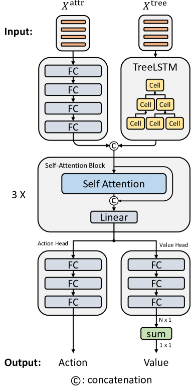
Figure 4: Overview of our network architecture. FC stands for fully connected layer.

TreeLSTM

LSTM (Hochreiter and Schmidhuber 1997), as a kind of RNN, was designed to deal with sequential data. Each LSTM cell takes state $(c_{t-1},h_{t-1})$ of last cell and a new $x_{t}$ as input, and output new cell state $c$ and $h$ to next cell.

$$(c_{t},h_{t})=\operatorname{LSTM-Cell}\left(x_{t},(c_{t-1},h_{t-1})\right)\\$$ (13)

Sequential data is a special case of trees, where each node has a unique child — its successor. Tai, Socher, and Manning modified its structure to deal with general trees in 2015. Tree differs from sequential data in the allowed number of children. Unlike sequential data, nodes in a tree are allowed to have multiple children. As a result, TreeLSTM receives a set of children’s output as input instead:

$$(c_{t},h_{t})=\operatorname{TreeLSTM-Cell}(x_{t},S_{t}),$$ (14)

where $S_{t}=\{(h_{k},c_{k})\;|\;k\in\operatorname{Child}(t)\}$. Within TreeLSTM cells, there are several ways to aggregate children’s states, leading to different variants of TreeLSTM. In our network, we adopt Child-sum TreeLSTM. See Tai, Socher, and Manning (2015) for detailed structures of TreeLSTM cells.

3.3 Reward Design

Agents are given rewards at every time step, according to their performance within the moment. Besides the normalized reward generated by the environment, agents are also rewarded when they depart from stations, arrive at targets, and get penalized when deadlocks happen. To promote cooperation between them, these rewards are shared by all agents, and no credit assignment is performed. As a result, a single agent is encouraged to wait for others if the waiting can lead to global efficiency improvement.

Environmental Reward

Agents are rewarded environmental reward $r^{(e)}_{t}$ at time step $t$:

$$r^{(e)}_{t}=\bar{R}_{t},$$ (15)

where $\bar{R}_{t}$ is the normalized environmental reward agents get in time step $t$.

Departure Reward

We reward agents when there are new agents departing:

$$r^{(d)}_{t}=\frac{n^{(d)}_{t}-n^{(d)}_{t-1}}{N},$$ (16)

where $n^{(d)}_{t}$ is the number of agents departing at or before time step $t$.

Arrival Reward

We reward agents when there are new arrivals:

$$r^{(a)}_{t}=\frac{n^{(a)}_{t}-n^{(a)}_{t-1}}{N},$$ (17)

where $n^{(a)}_{t}$ is the number of arrival so far at time step $t$.

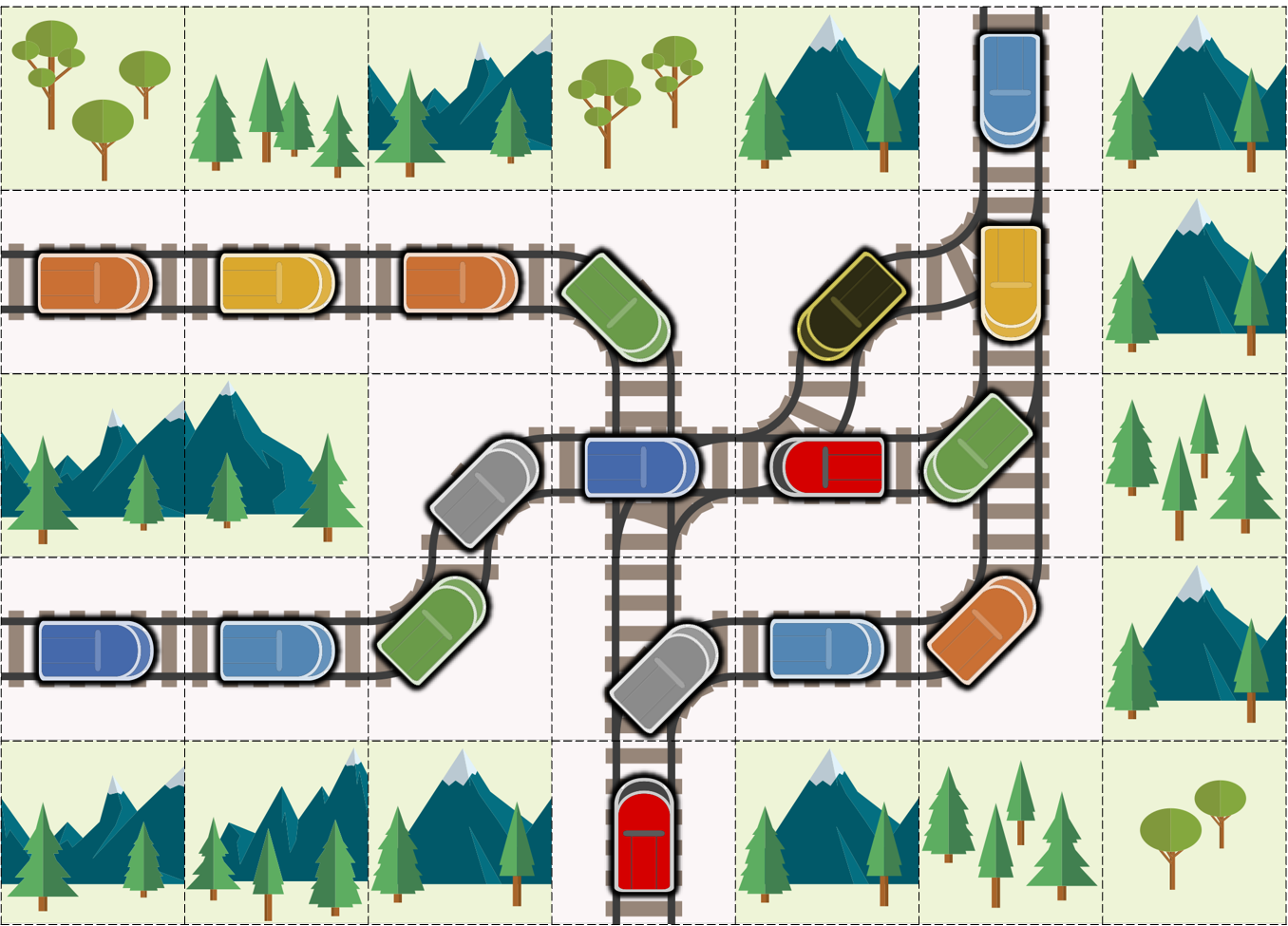
Figure 5: Because trains are not allowed to go backward, if two trains go into a single rail in opposite directions, a deadlock happens.

Deadlock Penalty

Because trains are not allowed to go backward, if two trains go into a single rail in opposite directions, a deadlock happens and no train can pass this rail again (see Figure 5). So, we give a penalty when new deadlocks happen:

$$r^{(l)}_{t}=\frac{n^{(l)}_{t}-n^{(l)}_{t-1}}{N},$$ (18)

where $n^{(l)}_{t}$ is the number of deadlocks on the map at time step $t$.

Total Reward

The final reward we give to agents at time $t$ is a weighted sum of all terms above:

$$r_{t}=c_{e}r_{t}^{(e)}+c_{a}r_{t}^{(a)}+c_{d}r_{t}^{(d)}-c_{l}r_{t}^{(l)},$$ (19)

where $c_{e},c_{a},c_{d},c_{l}$ are weight parameters.

4 Experiments

	#agents	Reward Weights				Initialized by
		$c_{e}$	$c_{a}$	$c_{d}$	$c_{l}$
Phase-I	50	1	5	0	2.5	N/A
Phase-II	50	0	5	1	2.5	Phase-I
Phase-III-50	50	0	5	1	2.5	Phase-II
Phase-III-80	80	1	5	0.1	2.5	Phase-III-50
Phase-III-100	100	1	5	0.1	2.5	Phase-III-50
Phase-III-200	200	1	5	0.1	2.5	Phase-III-100

Table 3: Settings of different phases.

	Arrival%	Env. Reward	Depart%
Phase-I	70.0	0.859	79.0
Phase-II	86.2	0.920	99.2

Table 4: Compare Phase-I and Phase-II.

Model	Phase-III-50		Phase-III-80
Test Stage	Arrival%	Env. Reward	Arrival%	Env. Reward
Test_04	50.5 $\pm$19.7	.781 $\pm$.079	62.6 $\pm$11.9	.812 $\pm$ .051
Test_05	49.4 $\pm$21.0	.779 $\pm$.073	62.9 $\pm$12.8	.824 $\pm$ .049
Test_06	51.6 $\pm$20.4	.788 $\pm$.083	70.6 $\pm$ 6.2	.859 $\pm$ .028
Test_07	52.2 $\pm$20.2	.803 $\pm$.086	65.4 $\pm$12.6	.833 $\pm$ .051
Test_08	52.9 $\pm$17.9	.789 $\pm$.083	74.3 $\pm$ 9.6	.877 $\pm$ .029

Table 5: Phase-III-50 is trained in 50-agent environments, but Test_04 to Test_08 are 80-agent environments. Model Phase-III-80 is initialized by Phase-III-50, and fine-tuned in 80-agent environments. After fine-tuning, both arrival ratios and environmental rewards increase significantly.

4.1 Experiment Settings

We largely followed the final round (round 2) configurations of the Flatland3 challenge to conduct experiments so that our results are comparable with the ones on the challenge leaderboard . There are 15 test stages in the final round, and each stage contains 10 test cases. Problem scales (Table 6) and difficulty gradually increase from initial stages to advanced stages. The first stage is the smallest one with 7 agents on a $30\times 30$ map, while the last stage contains 425 agents on a $158\times 158$ map. Teams’ submissions are tested stage by stage. A team can proceed to the next stage only if they pass the last stage (arrival ratio reaches 25%).

Test Stage	Model	#agents	Map Size	#cities	Arrival%	Env. Reward	Avg. Time/s
Test_00	Phase-III-50	7	$30\times 30$	2	$94.3\pm 10.0$	$.957\pm.030$	7.022
Test_01	Phase-III-50	10	$30\times 30$	2	$92.0\pm 9.2$	$.947\pm.047$	8.430
Test_02	Phase-III-50	20	$30\times 30$	3	$87.0\pm 13.6$	$.934\pm.063$	16.486
Test_03	Phase-III-50	50	$30\times 35$	3	$86.2\pm 10.2$	$.922\pm.047$	32.292
Test_04	Phase-III-80	80	$35\times 30$	5	$62.6\pm 11.9$	$.812\pm.051$	40.580
Test_05	Phase-III-80	80	$45\times 35$	7	$62.9\pm 12.8$	$.824\pm.049$	60.009
Test_06	Phase-III-80	80	$40\times 60$	9	$70.6\pm 6.2$	$.859\pm.028$	99.566
Test_07	Phase-III-80	80	$60\times 40$	13	$65.4\pm 12.6$	$.833\pm.051$	109.386
Test_08	Phase-III-80	80	$60\times 60$	17	$74.3\pm 9.6$	$.877\pm.029$	160.928
Test_09	Phase-III-100	100	$80\times 120$	21	$59.7\pm 15.7$	$.795\pm.067$	480.971
Test_10	Phase-III-100	100	$100\times 80$	25	$57.6\pm 16.7$	$.779\pm.067$	346.861
Test_11	Phase-III-200	200	$100\times 100$	29	$52.8\pm 5.8$	$.790\pm.033$	488.549
Test_12	Phase-III-200	200	$150\times 150$	33	$57.3\pm 5.0$	$.777\pm.037$	1314.509
Test_13	Phase-III-200	400	$150\times 150$	37	$34.9\pm 7.2$	$.704\pm.031$	2029.058
Test_14	Phase-III-200	425	$158\times 158$	41	$39.3\pm 9.7$	$.721\pm.038$	2329.925

Table 6: Performance of our models in 15 test stages.

Rank	Team	Tag	Score	Arv.%
1	An_Old_Driver	OR	141.0	88.0
2	Zain	OR	132.5	88.8
-	Ours	RL	125.3	66.4
3	SmartTrains	OR	118.0	76.9
4	dsa	OR	107.5	44.2
5	stavros_kakoulidis	other	40.5	55.6
6	UniTeam	other	29.9	39.1
7	WaveTeam	RL	27.9	38.6
8	SOBA	RL	27.8	32.6
9	ChewChewChew	RL	20.0	30.6
10	fridayPhenom	OR	6.9	18.6

Table 7: Compare our results with the top 10 in Flatland3 challenge leaderboard. The scores are collected by accumulating environmental rewards from all 15 test stages.

Test Stage	#agents	Arrival%	Env. Reward
Test_03	50	56.4 $\pm$ 10.8	.815 $\pm$ .038
Test_04	80	50.7 $\pm$ 9.6	.810 $\pm$ .023
Test_05	80	47.4 $\pm$ 9.0	.794 $\pm$ .021
Test_06	80	53.0 $\pm$ 8.0	.815 $\pm$ .041
Test_07	80	59.1 $\pm$ 7.9	.805 $\pm$ .041
Test_08	80	60.4 $\pm$ 6.0	.812 $\pm$ .021
Test_09	100	56.7 $\pm$ 10.3	.802 $\pm$ .035
Test_10	100	54.7 $\pm$ 3.9	.801 $\pm$ .031

Table 8: Performance of model Phase-III-200 in small environments. Generally, it performs worse than the scale-specific models in Table 6.

4.2 Multiple Phase Training

To reduce training difficulty, we train our models in curriculum learning style, and the whole training process can be roughly divided into three phases. In phases I and II, we train a model in 50-agent environments. We found that the learned model generalizes well to smaller environments but not larger ones. In phase III, models are initialized by the one learned in phase II and fine-tuned in settings with more agents.

Phase I

Initially, we only use the environmental reward, arrival reward, and deadlock penalty to encourage the trains to march on their targets and avoid deadlocks (see Phase-I in Table 3). After training, 70% agents in 50-agent environments can reach their targets, and a normalized reward of 0.859 is achieved. However, 21% agents have never departed because of the deadlock penalty. Agents choose not to depart and behave conservatively to avoid being penalized by deadlocks.

Phase II

In phase I, many trains do not depart, so we add a departure reward to encourage more departures (see Phase-II in Table 3). The experiment is initialized by the phase-I model, and after 5 days of training, its arrival ratio increases to 86.2%, and almost all the trains have departed (Table 4).

Phase III

Finally, we deal with environments with more than 80 agents. Training models in so large environments from scratch is very difficult, so we adopt curriculum learning. Models for large environments are initialized by parameters learned in small environments. Although models learned in small environments are able to directly generalize to large environments (Table 5), fine-tuning in large environments increases performances significantly.

4.3 Results and Analysis

Our stage-specific results are reported in Table 6; Final scores as well as top 10 teams’ scores in Flatland3 challenge are listed in Table 7. In summary, we scored 125.3, ranking top 2–3 on the leaderboard, while the best RL method before scored only 27.9. More specifically, we observe the following phenomena:

• No RL method before us managed to pass Test_03 stage, while our method passed all 15 stages.

• While the number of agents increases, model performance decreases, which suggests large-scale problems are more difficult than we expected.

• When the numbers of agents are equal (Test_04 to Test_08), model performance increases with a larger map and more cities because it leads to lower agent density and less traffic congestion.

• Compared to the third-best team, we achieved a higher environmental reward but a lower arrival ratio. This indicates that environmental rewards are not always consistent with arrival ratios because arrival ratios only care agents arrive or not while environmental rewards also care about how fast agents arrive. They are two highly related but different objectives. Similar phenomena can be observed in team An_Old_Driver and team Zain.

Generalization across environment scales

We are also interested in the generalization ability of our models and particularly interested in the generalization across environment scales. As Table 5 shows, models learned in small environments are able to generalize to large environments but perform worse than the one fine-tuned in large environments. Table 8 shows that models specialized in large environments are also able to generalize to small environments but perform worse than the ones learned in small environments. To achieve optimal performance, we need to train multiple scale-specific models.

Agent Cooperation

We observed many self-organized cooperative patterns in agents’ behaviors. They learn to line up to march in a compact manner (Figure 8). Fast ones learned to overtake the slow ones (Figure 6). Slow trains make way for fast ones (Figure 9). When there are two parallel rail lanes, trains spontaneously line up as if they are in a two-way street (Figure 8).

5 Conclusion

We provided a new RL solution to the Flatland3 challenge and achieved a score 4x better than the best RL method before. The key reasons behind the improvement are 1) the tree features and TreeLSTM we adopt and 2) the 20x faster feature parser, which enables us to train our model with far more data than the RL methods before. However, there is still a gap between our method and state-of-the-art OR methods (Li et al. 2021). Our method also takes longer time than OR methods. Another drawback is that there lacks a single model that is able to handle environments of any scale. To achieve optimal performance, we have to train multiple scale-specific models.

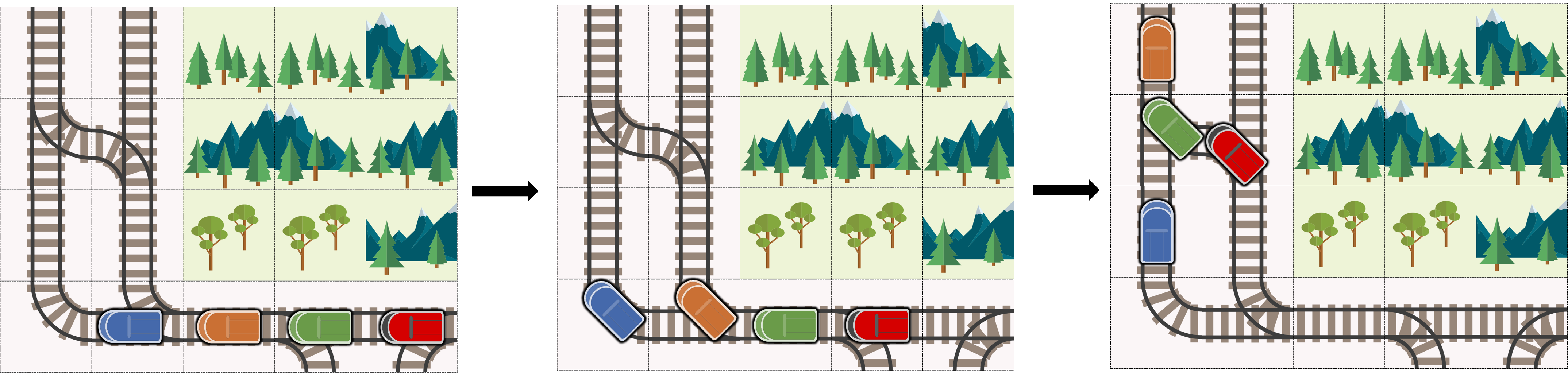
$T$                                                     $T+4$                                           $T+8$

Figure 6: Fast trains overtake the slow ones. The speed of the blue train is 0.25 while the other three are 1.0. Fast ones overtake the slow ones to reach targets earlier.

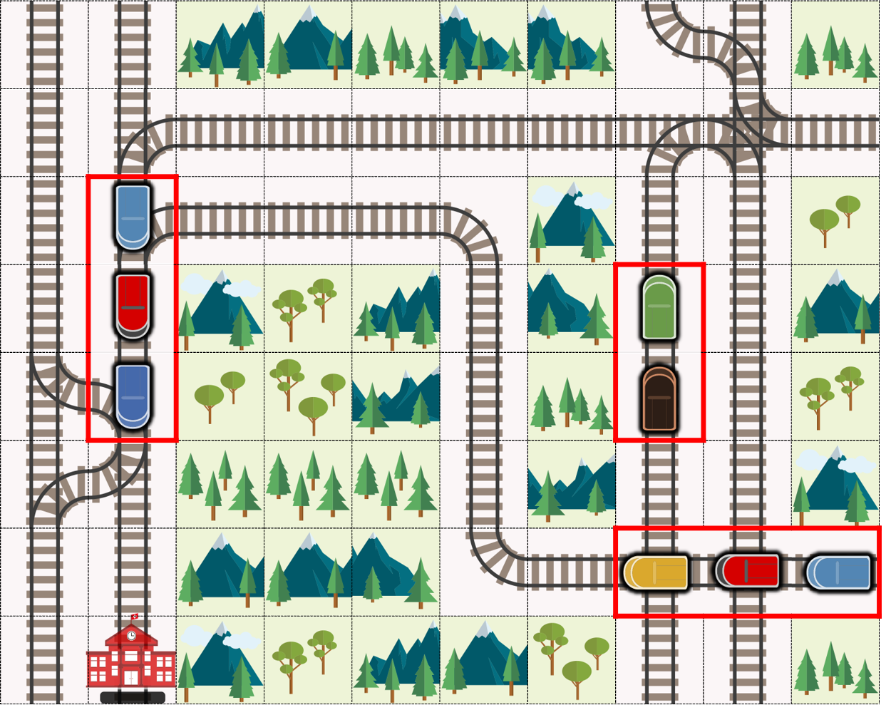
Figure 7: Trains line up in a row.

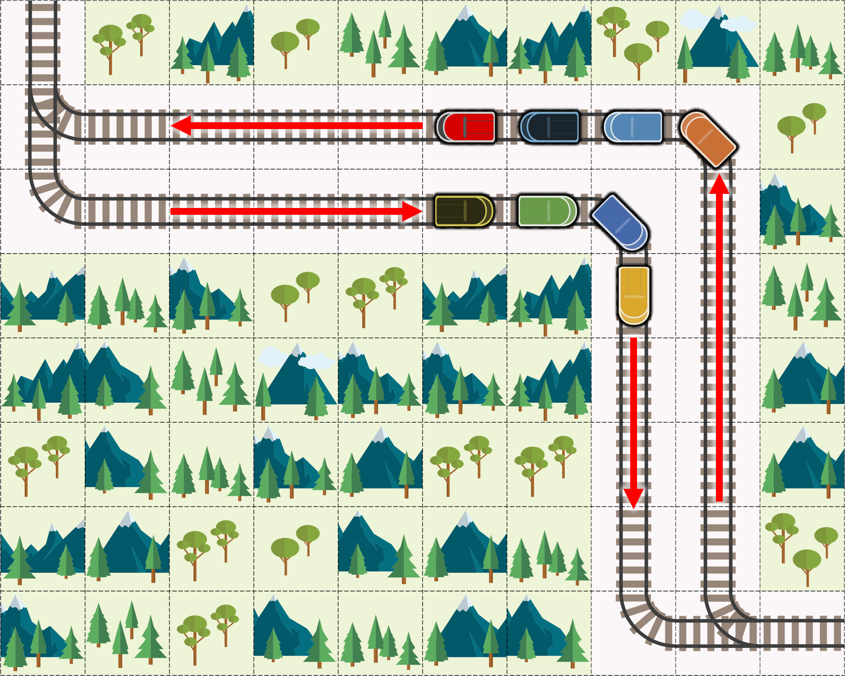
Figure 8: When there are two parallel rail lanes, trains spontaneously line up as if they are in a two-way street.

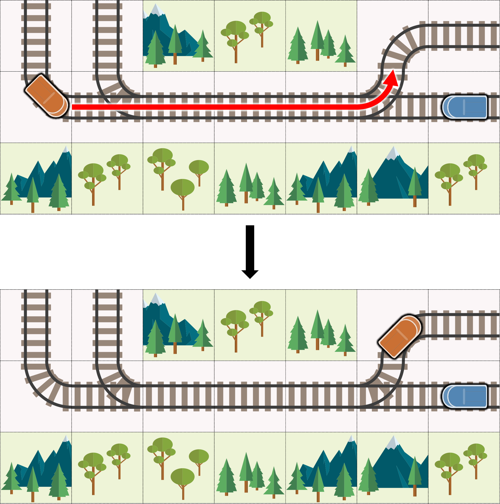
Figure 9: A slow train makes way for a fast one. The orange one has a speed of 1.0, and the blue one has a speed of 0.5. The blue one waits until the orange one passes.

References

- Berner et al. (2019) Berner, C.; Brockman, G.; Chan, B.; Cheung, V.; Debiak, P.; Dennison, C.; Farhi, D.; Fischer, Q.; Hashme, S.; Hesse, C.; et al. 2019. Dota 2 with large scale deep reinforcement learning. arXiv preprint arXiv:1912.06680.
- Cohen et al. (2019) Cohen, L.; Uras, T.; Kumar, T. S.; and Koenig, S. 2019. Optimal and bounded-suboptimal multi-agent motion planning. In Twelfth Annual Symposium on Combinatorial Search.
- Hochreiter and Schmidhuber (1997) Hochreiter, S.; and Schmidhuber, J. 1997. Long short-term memory. Neural computation, 9(8): 1735–1780.
- Laurent et al. (2021) Laurent, F.; Schneider, M.; Scheller, C.; Watson, J.; Li, J.; Chen, Z.; Zheng, Y.; Chan, S.-H.; Makhnev, K.; Svidchenko, O.; Egorov, V.; Ivanov, D.; Shpilman, A.; Spirovska, E.; Tanevski, O.; Nikov, A.; Grunder, R.; Galevski, D.; Mitrovski, J.; Sartoretti, G.; Luo, Z.; Damani, M.; Bhattacharya, N.; Agarwal, S.; Egli, A.; Nygren, E.; and Mohanty, S. 2021. Flatland Competition 2020: MAPF and MARL for Efficient Train Coordination on a Grid World. In Proceedings of the NeurIPS 2020 Competition and Demonstration Track, volume 133 of Proceedings of Machine Learning Research, 275–301.
- Li et al. (2021) Li, J.; Chen, Z.; Zheng, Y.; Chan, S.-H.; Harabor, D.; Stuckey, P. J.; Ma, H.; and Koenig, S. 2021. Scalable Rail Planning and Replanning: Winning the 2020 Flatland Challenge. In Proceedings of the International Conference on Automated Planning and Scheduling (ICAPS), 477–485.
- Ma, Kumar, and Koenig (2017) Ma, H.; Kumar, T. S.; and Koenig, S. 2017. Multi-agent path finding with delay probabilities. In Proceedings of the AAAI Conference on Artificial Intelligence, volume 31.
- Ma et al. (2018) Ma, H.; Wagner, G.; Felner, A.; Li, J.; Kumar, T.; and Koenig, S. 2018. Multi-agent path finding with deadlines. arXiv preprint arXiv:1806.04216.
- Mohanty et al. (2020) Mohanty, S.; Nygren, E.; Laurent, F.; Schneider, M.; Scheller, C.; Bhattacharya, N.; Watson, J.; Egli, A.; Eichenberger, C.; Baumberger, C.; et al. 2020. Flatland-RL: Multi-agent reinforcement learning on trains. arXiv preprint arXiv:2012.05893.
- Nebel (2020) Nebel, B. 2020. On the computational complexity of multi-agent pathfinding on directed graphs. In Proceedings of the International Conference on Automated Planning and Scheduling, volume 30, 212–216.
- Schulman et al. (2017) Schulman, J.; Wolski, F.; Dhariwal, P.; Radford, A.; and Klimov, O. 2017. Proximal Policy Optimization Algorithms. ArXiv, abs/1707.06347.
- Silver et al. (2017) Silver, D.; Schrittwieser, J.; Simonyan, K.; Antonoglou, I.; Huang, A.; Guez, A.; Hubert, T.; Baker, L.; Lai, M.; Bolton, A.; et al. 2017. Mastering the game of go without human knowledge. nature, 550(7676): 354–359.
- Švancara et al. (2019) Švancara, J.; Vlk, M.; Stern, R.; Atzmon, D.; and Barták, R. 2019. Online multi-agent pathfinding. In Proceedings of the AAAI conference on artificial intelligence, volume 33, 7732–7739.
- Tai, Socher, and Manning (2015) Tai, K. S.; Socher, R.; and Manning, C. D. 2015. Improved Semantic Representations From Tree-Structured Long Short-Term Memory Networks. In Proceedings of the 53rd Annual Meeting of the Association for Computational Linguistics and the 7th International Joint Conference on Natural Language Processing (Volume 1: Long Papers), 1556–1566.
- Vaswani et al. (2017) Vaswani, A.; Shazeer, N.; Parmar, N.; Uszkoreit, J.; Jones, L.; Gomez, A. N.; Kaiser, Ł.; and Polosukhin, I. 2017. Attention is all you need. Advances in neural information processing systems, 30.
- Vinyals et al. (2019) Vinyals, O.; Babuschkin, I.; Czarnecki, W. M.; Mathieu, M.; Dudzik, A.; Chung, J.; Choi, D. H.; Powell, R.; Ewalds, T.; Georgiev, P.; et al. 2019. Grandmaster level in StarCraft II using multi-agent reinforcement learning. Nature, 575(7782): 350–354.