Synchronization in a Kuramoto Mean Field Game

Abstract

The classical Kuramoto model is studied in the setting of an infinite horizon mean field game. The system is shown to exhibit both synchronization and phase transition. Incoherence below a critical value of the interaction parameter is demonstrated by the stability of the uniform distribution. Above this value, the game bifurcates and develops self-organizing time homogeneous Nash equilibria. As interactions become stronger, these stationary solutions become fully synchronized. Results are proved by an amalgam of techniques from nonlinear partial differential equations, viscosity solutions, stochastic optimal control and stochastic processes.

Key words: Mean field games, Kuramoto model, Synchronization, viscosity solutions.
Mathematics Subject Classification: 35Q89, 35D40, 39N80, 91A16, 92B25

1 Introduction

Originally motivated by systems of chemical and biological oscillators, the classical Kuramoto model [17] has found an amazing range of applications from neuroscience to Josephson junctions in superconductors, and has become a key mathematical model to describe self organization in complex systems. These autonomous oscillators are coupled through a nonlinear interaction term which plays a central role in the long time behavior of the system. While the system is unsynchronized when this term is not sufficiently strong, fascinatingly they exhibit an abrupt transition to self organization above a critical value of the interaction parameter. Synchronization is an emergent property that occurs in a broad range of complex systems such as neural signals, heart beats, fire-fly lights and circadian rhythms. Expository papers [1, 21] and the references therein provide an excellent introduction to the model and its applications.

The analysis of the coupled Kuramoto oscillators through a mean field game formalism is first explored by [22, 23] proving bifurcation from incoherence to coordination by a formal linearization and a spectral argument. [6] further develops this analysis in their application to a jet-lag recovery model. We follow these pioneering studies and analyze the Kuramoto model as a discounted infinite horizon stochastic game in the limit when the number of oscillators goes to infinity. We treat the system of oscillators as an infinite particle system, but instead of positing the dynamics of the particles, we let the individual particles endogenously determine their behaviors by minimizing a cost functional and hopefully, settling in a Nash equilibrium. Once the search for equilibrium is recast in this way, equilibria are given by solutions of nonlinear systems. Analytically, they are characterized by a backward dynamic programming equation coupled to a forward Fokker-Planck-Kolmogorov equation, and in the probabilistic approach, by forward-backward stochastic differential equations. Stability analysis of the solutions is delicate because of this forward-backward nature of the solution, and to the best of our knowledge, it remains a challenging problem. Except possibly in the finite horizon potential case (cf. [3] and the references therein) it has not been fully addressed in the existing literature on the subject. For the stability results of the Kuramoto model in the classical setting, the interested reader could consult [14, 15] and the references therein.

With finitely many oscillators, we consider the following version of the model already introduced in [6, 23]. We fix a large integer $N$ and for $i\in\{1,\dots,N\}$ let $\theta^{i}_{t}$ be the phase of the $i$-th oscillator at time $t\geq 0$. We assume the phases $\theta^{i}_{t}$ are controlled Ito diffusion processes satisfying, $\mathrm{d}\theta^{i}_{t}=\alpha^{i}_{t}\mathrm{d}t+\sigma\mathrm{d}B^{i}_{t}$, where $B^{i}$’s are independent Brownian motions, and the control processes $\alpha^{i}$ are exerted by the individual oscillators so as to simultaneously minimize their costs given by

$$\alpha^{i}\mapsto J^{i}(\boldsymbol{\alpha}):=\mathbb{E}\int_{0}^{\infty}e^{-\beta t}\left[\kappa\;L(\theta^{i}_{t},\boldsymbol{\theta}_{t})+\tfrac{1}{2}(\alpha^{i}_{t})^{2}\right]\mathrm{d}t,$$

where $\boldsymbol{\alpha}=(\alpha^{1},\ldots,\alpha^{N})$ and $\boldsymbol{\theta}_{t}=(\theta^{1}_{t},\ldots,\theta^{N}_{t})$. The positive constants $\sigma,\beta$ are respectively, the common standard deviations of the random shocks affecting the dynamics of the phases, and the common discounting factor used to compute the present value of the cost. The centrally important positive constant $\kappa$ models the strength of the interactions between the oscillators.

In line with the classical literature on Kuramoto’s synchronization theory, we assume that the running cost function $L$ is given by

$$L(\theta^{i},\boldsymbol{\theta}) =\frac{1}{N}\sum_{j\neq i}{2\left(\sin\left((\theta^{i}-\theta^{j})/2\right)\right)^{2}}=\frac{1}{N}\sum_{j=1}^{N}{2\left(\sin\left((\theta^{i}-\theta^{j})/2\right)\right)^{2}}.$$

The cost $L$ accounts for the cooperation between the $N$ oscillators by incentivizing them to align their frequencies, while the term $(\alpha^{i}_{t})^{2}$ represents a form of kinetic energy which is also to be minimized. It is convenient to express the above cost functional by using the empirical distribution measure of the oscillators as follows,

$$L(\theta^{i}_{t},\boldsymbol{\theta}_{t})=c(\theta^{i}_{t},\bar{\mu}^{N}_{t}),\qquad\text{where}\qquad c(\theta,\mu):=\int{2\left(\sin\left((\theta-\theta^{\prime})/2\right)\right)^{2}}\,\mu(\mathrm{d}\theta^{\prime}),$$ (1.1)

and the empirical measure $\bar{\mu}^{N}_{t}$ is given by,

$$\bar{\mu}^{N}_{t}=\bar{\mu}(\boldsymbol{\theta}_{t}):=\frac{1}{N}\sum_{j=1}^{N}\delta_{\theta^{j}_{t}}.$$

As the finite particle system is essentially intractable, especially for large values of $N$, we follow approach of [4, 5, 16, 18, 19, 20] that is now considered standard, and approximate the Nash equilibria for the above system of oscillators by letting their number $N$ go to infinity. Then, for a given flow of probability measures $\boldsymbol{\mu}=(\mu_{t})_{t\geq 0}$, the stochastic optimal control problem for the representative oscillator is to minimize

$$\alpha\in{\mathcal{A}}\ \mapsto\mathbb{E}\int_{0}^{\infty}e^{-\beta t}\left(\ell(t,X_{t})+\frac{1}{2}\alpha^{2}_{t}\right)\mathrm{d}t,$$ (1.2)

where ${\mathcal{A}}$ is the set of all right-continuous and progressively measurable processes, the running cost $\ell(t,x)$ is equal to $\kappa c(x,\mu_{t})$ with $c$ as in (1.1), and $X_{t}$ is the controlled phase of the representative oscillator given by $X_{t}=X_{0}+\int_{0}^{t}{\alpha_{u}\mathrm{d}u}+\sigma B_{t}$, for a Brownian motion $B_{t}$. The Nash equilibrium, as defined in Definition 3.1 below, is achieved when the flow $\boldsymbol{\mu}=(\mu_{t})_{t\geq 0}$ is given by the marginal laws of the optimal process $X^{*}_{t}$. By direct methods, Lemma 4.5 proves the existence of such equilibrium flows starting from any initial distribution.

It is immediate that the uniform distribution $U(\mathrm{d}x)=\mathrm{d}x/(2\pi)$ on the torus gives a stationary equilibrium flow. Indeed, $c(x,U)\equiv 1$ and therefore, the optimal control for the above problem with the constant flow $U$ is identically equal to zero. As the uniform distribution has no special structure, it represents incoherence among the oscillators, and when the interaction parameter is small, we show that all the solutions of the Kuramoto mean field game converge to this incoherent state. This global attraction is proved in Lemma 4.3 for $\kappa<\beta\sigma^{2}/4$. Theorem 4.4 considers all $\kappa$ less than the critical value

$$\kappa_{c}:=\beta\sigma^{2}+\sigma^{4}/2,$$ (1.3)

and proves that there are that start “close” to the uniform distribution converge to it as time tends to infinity. Thus, Lemma 4.3 and Theorem 4.4 reveal that incoherence is the main paradigm in the sub-critical regime $\kappa<\kappa_{c}$. Theorem 4.1 analyzes the case $\kappa>\kappa_{c}$, and proves that there are infinitely many self-organizing stationary solutions for these interaction parameter values. In particular, these solutions do not converge to the incoherent uniform distribution and numerically they are stable. Hence, $\kappa_{c}$ is a sharp threshold for the stability of incoherence, and there is a phase transition from total disorder to self organization exactly at this critical interaction parameter $\kappa_{c}$. Furthermore, Theorem 4.2 shows convergence to full synchronization as $\kappa$ gets larger.

The classical Kuramoto model with noise has been the object of many studies, and the mean field version is the following McKean-Vlasov stochastic differential equation

$$\mathrm{d}X_{t}=-\kappa\ \int_{\mathbb{T}}{\sin(X_{t}-y){\mathcal{L}}(X_{t})(\mathrm{d}y)}\ \mathrm{d}t+\sigma\mathrm{d}B_{t},$$

where ${\mathcal{L}}(X_{t})$ is the law of the random variable $X_{t}$. The uniform distribution is shown in [12] to be both locally and globally stable when $\kappa<\sigma^{2}$. The corresponding finite particle system is studied in [2, 8]. There, it is proven that the solutions of the finite model remain close to the solution of the above equation for a very long time, on the order of $o(\exp(N))$. Similar results are also proved for the Kuramoto mean field game with an ergodic cost in [23], by using bifurcation theory techniques including the Lyapunov-Schmidt reduction method to show the existence of non-uniform stationary solutions near the critical value $\kappa^{*}_{c}=\sigma^{4}/2$. Rabinowitz bifurcation theorem and other global techniques are used in [7] for similar results.

The classical Kuramoto model and its mean field game versions provide a mechanism for the analysis of self organization. However, they cannot model synchronization with external drivers, thus requiring additional terms. Indeed, the jet-lag recovery model of [6] introduce a cost for misalignment with the exogenously given sunlight frequency, providing an incentive to be in synch with the environment as well. These studies are clear evidences of the modeling potential of the mean field game formalism in all models when self organization is the salient feature.

The paper is organized as follows. After a short section on notation, the Kuramoto mean field game is introduced in Section 3, and the main results are stated in Section 4. Section 5 briefly summarizes all control problems used in the paper. Stationary solutions are defined and a fixed-point characterization is proved in Section 6. The super-critical case is studied in Section 7 and full synchronization in Section 8. Incoherence is demonstrated in Section 9 by proving the convergence of all solutions to the uniform distribution when the interaction parameter is small, and local stability of the uniform distribution is established in Section 10 for all $\kappa<\kappa_{c}$. For completeness, solutions starting from any distribution are constructed in the Appendix A, and we provide the expected comparison result for a degenerate Eikonal equation in the Appendix B.

2 Notation

The state-space is the one-dimensional torus $\mathbb{T}:=\mathbb{R}/(2\pi\mathbb{Z})$, ${\mathcal{P}}(\mathbb{T})$ is the space of all probability measures on $\mathbb{T}$. For $\nu\in{\mathcal{P}}(\mathbb{T})$, $f\in C(\mathbb{T})$, we use the standard notation $\nu(f):=\int_{\mathbb{T}}\,f(x)\,\nu(dx).$ We say that a probability measure $\nu\in{\mathcal{P}}(\mathbb{T})$ is the law ${\mathcal{L}}(X)$ of $X$, if $\mathbb{E}[f(X)]=\nu(f)$ for every $f\in C(\mathbb{T})$. We also use the following space of continuous functions,

$${\mathcal{C}}:=\{\ \xi=(\gamma,\eta):[0,\infty)\mapsto\mathbb{R}^{2}\ :\ \text{continuous and bounded}\ \}.$$

We fix a filtered probability space $(\Omega,\mathbb{F},\mathbb{P})$ supporting an $\mathbb{F}$-adapted Brownian motion $(B_{t})_{t\geq 0}$. We assume that the filtration $\mathbb{F}=\{{\mathcal{F}}_{t}\}_{t\geq 0}$ satisfies the usual conditions, i.e. ${\mathcal{F}}_{0}$ is complete and ${\mathcal{F}}_{t}$ is right-continuous. The initial filtration is non-trivial so that for any probability measure $\mu_{0}\in{\mathcal{P}}(\mathbb{T})$, one can construct an ${\mathcal{F}}_{0}$ measurable, $\mathbb{T}$ valued random variable $X_{0}$ with distribution $\mu_{0}$. For $t\geq 0$, the set ${\mathcal{A}}_{t}$ of all progressively measurable processes $\alpha:[t,\infty)\to\mathbb{R}$ is called the admissible controls, and we set ${\mathcal{A}}:={\mathcal{A}}_{0}$.

For $\mu\in{\mathcal{P}}(\mathbb{T}),z\in\mathbb{T}$ and a Borel subset $B\subset\mathbb{T}$, we define the translation of $\mu$ by,

$$\mu(B;x):=\mu(\{z\in\mathbb{T}\ :\ x+z\in B\ \}).$$ (2.1)

Finally, we record several elementary trigonometric identities that are used repeatedly. For $\mu\in{\mathcal{P}}(\mathbb{T})$, let $c(x,\mu)$ be as in the Introduction. As $2\left(\sin\left(x/2\right)\right)^{2}=1-\cos(x)$,

$$c(x,\mu)=\int_{\mathbb{T}}2\left(\sin\left((x-y)/2\right)\right)^{2}\,\mu(\mathrm{d}y)=1-a(\mu)\cos(x)-b(\mu)\sin(x),$$ (2.2)

where $a(\mu):=\mu(\cos)$, and $b(\mu):=\mu(\sin)$. In particular, there is $z^{*}\in\mathbb{T}$ such that

$$a(\mu(\cdot;z^{*}))=g(\mu):=\sqrt{(a(\mu))^{2}+(b(\mu))^{2}\ },\qquad\text{and}\qquad b(\mu(\cdot;z^{*}))=0.$$ (2.3)

3 Kuramoto mean-field game

Given a flow of probability measures $\boldsymbol{\mu}=(\mu_{t})_{t\geq 0}$, set

$$\ell_{\boldsymbol{\mu}}(t,x):=\kappa[c(x,\mu_{t})-1]=-\kappa\mu_{t}(\cos)\cos(x)-\kappa\mu_{t}(\sin)\sin(x),\qquad x\in\mathbb{T},t\geq 0.$$

Consider the optimal control problem (1.2) with this running cost. Then, the problem is

$$v_{\boldsymbol{\mu}}:=\inf_{\alpha\in{\mathcal{A}}}J_{{\boldsymbol{\mu}},\kappa}(\alpha):=\inf_{\alpha\in{\mathcal{A}}}\mathbb{E}\int_{0}^{\infty}e^{-\beta t}\left(\ell_{\boldsymbol{\mu}}(t,X^{\alpha}_{t})+\frac{1}{2}\alpha^{2}_{t}\right)\mathrm{d}t,$$ (3.1)

where as in the Introduction, $X^{\alpha}_{t}:=X_{0}+\int_{0}^{t}{\alpha_{u}\mathrm{d}u}+\sigma B_{t}$, with a Brownian motion $(B_{t})_{t\geq 0}$ and an initial condition $X_{0}$ satisfying ${\mathcal{L}}(X_{0})=\mu_{0}$.

Definition 3.1.

We say that $\boldsymbol{\mu}=(\mu_{t})_{t\geq 0}$ is a solution to the Kuramoto mean-field game with interaction parameter $\kappa$ starting from initial distribution $\mu_{0}$, if there exists $\alpha^{*}\in{\mathcal{A}}$ such that $J_{{\boldsymbol{\mu}},\kappa}(\alpha^{*})=\inf_{\alpha\in{\mathcal{A}}}J_{{\boldsymbol{\mu}},\kappa}(\alpha)$ and $\mu_{t}={\mathcal{L}}(X^{\alpha^{*}}_{t})$ for all $t\geq 0$.

Example 3.2.

Consider an initial condition $X_{0}$ satisfying $\mathbb{E}\cos(X_{0})=\mathbb{E}\sin(X_{0})=0$, and the flow of probability measures $\boldsymbol{\mu}=(\mu_{t})_{t\geq 0}$ with $\mu_{t}:={\mathcal{L}}(X_{0}+\sigma B_{t}).$ Then, for every $t\geq 0$,

$$\ell_{\boldsymbol{\mu}}(t,x) =-\kappa(\mu_{t}(\cos)\cos(x)+\mu_{t}(\sin)\sin(x))$$

$$=-\kappa(\ \cos(x)\mathbb{E}[\cos(X_{0}+\sigma B_{t})]+\sin(x)\mathbb{E}[\sin(X_{0}+\sigma B_{t})])$$

$$=-\kappa(\cos(x)e^{-\frac{\sigma^{2}}{2}t}\mathbb{E}[\cos(X_{0})]-\sin(x)e^{-\frac{\sigma^{2}}{2}t}\mathbb{E}[\sin(X_{0})])=0.$$

Therefore, for any $\alpha\in{\mathcal{A}}$, $J_{{\boldsymbol{\mu}},\kappa}(\alpha)=\mathbb{E}\int_{0}^{\infty}e^{-\beta t}\ \frac{\alpha^{2}_{t}}{2}\ \mathrm{d}t\geq 0=J_{{\boldsymbol{\mu}},\kappa}(0)$, implying that $\alpha^{*}\equiv 0$ is the minimizer of $J_{{\boldsymbol{\mu}},\kappa}(\alpha)$, and $\boldsymbol{\mu}$ is the law of the dynamics controlled by $\alpha^{*}$. Hence, $\boldsymbol{\mu}$ is a solution of the Kuramoto mean-field game for every $\kappa$.

Now suppose that ${\mathcal{L}}(X_{0})$ is the uniform probability measure on the torus $U(\mathrm{d}x)=\mathrm{d}x/(2\pi)$. As any translation of $U$ is equal to itself, $\mu_{t}={\mathcal{L}}(X_{0}+\sigma B_{t})=U$ for all $t\geq 0$. Thus, $U$ is a stationary solution. ∎

The uniform distribution represents complete incoherence, and we refer to it as the incoherent (or uniform) solution. We next introduce the stationary solutions of the Kuramoto mean-field games.

Definition 3.3.

We call a probability measure $\mu\in{\mathcal{P}}(\mathbb{T})$ a stationary solution if the constant flow $\boldsymbol{\mu}=(\mu_{t})_{t\geq 0}$ with $\mu_{t}=\mu$ for all $t\geq 0$ is a solution of the Kuramoto mean-field game. We say that $\mu$ is self-organizing or non-uniform if it is not equal to the uniform measure $U$.

We record the following simple result for future reference.

Lemma 3.4.

The uniform probability measure $U$ on the torus is the incoherent stationary solution of the Kuramoto mean-field game. Moreover, a stationary solution $\mu$ is the uniform probability measure if and only if $\mu(\cos)=\mu(\sin)=0$.

Proof.

In Example 3.2, we have shown that $U$ is a stationary solution and that $c(\cdot,U)\equiv 1$. Now suppose that $\mu$ is a stationary solution with $\mu(\cos)=\mu(\sin)=0$. Then, as in Example 3.2, we conclude that the optimal solution of the control problem (1.2) is $\alpha^{*}\equiv 0$, and the optimal state process satisfies $\mathrm{d}X^{*}_{t}=\sigma\mathrm{d}B_{t}$. As by stationarity ${\mathcal{L}}(X^{*}_{t})=\mu$ for every $t\geq 0$, the density $f$ of $\mu$ solves the Fokker-Plank equation $f_{xx}(x)=0$ on the torus. Hence, $f$ is equal to a constant, and $\mu=U$. ∎

Remark 3.5 (Invariance by translation).

Assume that $\mu$ is a stationary solution. The symmetry of the problem implies that the translated measure $\mu(\cdot;z)$ is also a stationary solution for every $z$. ∎

4 Main Results

In this section, we state all the main results of the paper. Recall the critical interaction parameter $\kappa_{c}$ of (1.3). In Section 7, we study the super-critical case $\kappa>\kappa_{c}$, and prove the following result.

Theorem 4.1 (Super-critical interaction: synchronization).

For all interaction parameters $\kappa>\kappa_{c}$, there are non-uniform stationary solutions of the Kuramoto mean field game.

Suppose $\mu$ is one of the non-uniform stationary solutions given by the above result. Then, any translation $\mu(\cdot;z)$ is also a stationary solution. We conjecture that up to these translations, there exists a unique non-uniform stationary solution of the Kuramoto mean-field game for every interaction parameter $\kappa>\kappa_{c}$, see Remark 7.4 below.

We interpret these non-uniform stationary solutions as partially organized states of the Kuramoto mean-field game, and conclude that for interaction parameters $\kappa$ larger than the critical value $\kappa_{c}$, there is self organization. As $\kappa$ gets larger the stationary measure become more localized and Theorem 4.2, proved in Section 8 below, shows convergence to the fully synchronized regime corresponding to stationary Dirac measures.

Theorem 4.2 (Strong interaction: full synchronization).

Let $\mu_{n}$ be a sequence of non-uniform stationary solutions of the Kuramoto mean-field game with interaction parameters $\kappa_{n}$ tending to infinity. Then, there exists a sequence $z_{n}\in\mathbb{T}$ such that the translated stationary solutions $\mu_{n}(\cdot\ ;z_{n})$ converge in law to the Dirac measure $\delta_{\{0\}}$.

We have already argued in Example 3.2 that the uniform measure is always a stationary solution for all interaction parameters. In Section 9 below, we consider small interaction parameters and prove that all solutions converge to this incoherent state.

Lemma 4.3 (Weak interaction: incoherence).

If $\kappa<\beta\sigma^{2}/4$, then any solution $\boldsymbol{\mu}=(\mu_{t})_{t\geq 0}$ of the Kuramoto mean field game with interaction parameter $\kappa$ converges to the incoherent state, i.e., as $t$ tends to infinity, $\mu_{t}$ converges in law to $U$.

The next result, proved in Section 10, addresses the local stability for all $\kappa<\kappa_{c}$, showing that a phase transition occurs exactly at $\kappa_{c}$. This result require the initial distribution $\mu_{0}$ to be sufficiently close to the uniform distribution. To quantify the distance of any measure $\mu_{0}\in{\mathcal{P}}(\mathbb{T})$ to the uniform measure, we set

$$d(\mu_{0}):=\max\left\{|\mu_{0}(\cos)|\,,\,|\mu_{0}(\sin)|\,,\,|\mu_{0}(\sin\cos)|\,,\,|\mu_{0}(\cos^{2})-\tfrac{1}{2}|\,\right\}.$$ (4.1)

Theorem 4.4 (Sub-critical interaction: desynchronization).

For $\kappa<\kappa_{c}$, there is $c_{\kappa}$ such that for every $\mu_{0}\in{\mathcal{P}}(\mathbb{T})$ satisfying $d(\mu_{0})\leq c_{\kappa}$, there exists a solution $\boldsymbol{\mu}^{*}=(\mu^{*}_{t})_{t\geq 0}$ of the Kuramoto mean field game with interaction parameter $\kappa$ and initial distribution $\mu_{0}$, such that $\mu^{*}_{t}$ converges in law to the uniform distribution as $t$ tends to infinity. Moreover, this convergence is exponential in the sense that for some $\lambda^{*}_{\kappa}>0$,

$$\sup_{t\geq 0}\,e^{\lambda^{*}_{\kappa}t}\,d(\mu^{*}_{t})<\infty.$$ (4.2)

The existence of solutions to mean field games is well known for problems with ergodic cost [18, 19, 20]. However, for discounted infinite horizon problems it follows directly from our general approach. Thus, we provide this proof for completeness in the Appendix A.

Lemma 4.5 (Existence of solutions).

For any probability measure $\mu_{0}\in{\mathcal{P}}(\mathbb{T})$ and $\kappa\geq 0$, there exists a solution $\boldsymbol{\mu}=(\mu_{t})_{t\geq 0}$ of the Kuramoto mean field game with interaction parameter $\kappa$ starting from initial distribution $\mu_{0}$.

4.1 Illustration of the results

To illustrate our main results numerically, we consider the problem with parameters $\beta=1/2$, $\sigma=1$ with critical value $\kappa_{c}=1$. We numerically compute the solutions of the Kuramoto mean field game with two interaction parameters.

The first case $\kappa=0.8$ is below the threshold, and we are in the regime considered in Theorem 4.4. We compute a solution with initial condition $\nu(\mathrm{d}x)=C\exp\left(-\sin(x)\right)\mathrm{d}x$. Left panel in Figure 1 illustrates the convergence of the solution to the uniform distribution.

The case $\kappa=2$ is above the critical value and Theorem 4.1 implies that there are non-uniform stationary solutions. Indeed, we compute a solution of the Kuramoto mean field game with initial distribution that have two clusters around $\pi/2$ and $3\pi/2$,

$$\nu(\mathrm{d}x)=C\,\chi_{[\pi/4,\pi/4+\pi/10]\cup[\pi,\pi+\pi/10]}(x)\,\mathrm{d}x.$$

As seen in the right panel of Figure 1, the two clusters quickly merge and the solution converges towards a non-uniform invariant probability measure, whose shape is reported Figure 2.

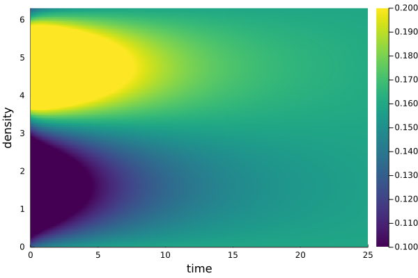
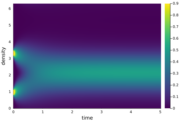
Figure 1: Left panel sub critical interaction, right panel super critical.

In all our numerical experiments with $\kappa>\kappa_{c}$, the solutions converge to shifts of the solutions constructed in the proof of Theorem 4.1. The exact translation is determined by the initial distribution. We do not provide a study of this interesting phenomenon.

5 Control problems

The original and the central stochastic optimal control problem is defined in (3.1). However, in the sequel, we use several other closely related problems in our analysis. So to highlight the subtle differences among them and to provide a general overview of the notation, we define all of them in this section. It is also clear that adding a constant to the running cost of any control problem does not alter the minimizing control. As we are only interested in the optimal behavior, we use this flexibility and appropriately modify the problem whenever it is convenient.

5.1 Inhomogeneous problems

For $\xi=(\gamma,\eta)\in{\mathcal{C}}$, we consider the stochastic control

$$v_{\xi}(\mu_{0}):=\inf_{\alpha\in{\mathcal{A}}}J_{\xi}(\mu_{0},\alpha):=\inf_{\alpha\in{\mathcal{A}}}\mathbb{E}\int_{0}^{\infty}e^{-\beta t}\left(\ell_{\xi}(t,X^{\alpha}_{t})+\frac{1}{2}\alpha^{2}_{t}\right)\mathrm{d}t,$$ (5.1)

where $X^{\alpha}_{t}:=X_{0}+\int_{0}^{t}{\alpha_{u}\mathrm{d}u}+\sigma B_{t}$ is as before with initial data satisfying ${\mathcal{L}}(X_{0})=\mu_{0}$, and the running cost is given by,

$$\ell_{\xi}(t,x)=-\gamma(t)\cos(x)-\eta(t)\sin(x),\qquad x\in\mathbb{T},t\geq 0.$$ (5.2)

We let $X^{\xi}$ be the optimal state process. The dependence on $\mu_{0}$ through the condition ${\mathcal{L}}(X^{\xi}_{0})=\mu_{0}$ is omitted in the notation for simplicity. To characterize the dynamics of $X^{\xi}$, we also need to introduce a family of control problems starting from any pair $(t,x)\in[0,\infty)\times\mathbb{T}$. Recall that ${\mathcal{A}}_{t}$ is the set of all adapted control process $\alpha:[t,\infty)\mapsto\mathbb{R}$. We set

$$v^{\xi}(t,x):=\inf_{\alpha\in{\mathcal{A}}_{t}}J_{\xi}(t,x,\alpha):=\inf_{\alpha\in{\mathcal{A}}_{t}}\mathbb{E}\int_{t}^{\infty}e^{-\beta(u-t)}[\ell_{\xi}(u,X^{\alpha,(t,x)}_{u})+\tfrac{1}{2}\alpha_{u}^{2}]\ \mathrm{d}u,$$ (5.3)

where

$$X^{\alpha,(t,x)}_{u}=x+\int_{t}^{u}{\alpha_{s}\mathrm{d}s}+\sigma[B_{u}-B_{t}],\qquad u\geq t.$$ (5.4)

We use the notation $X^{\alpha,x}=X^{\alpha,(0,x)}$. For a given process $\xi$, let $\alpha^{*}$ be the optimal control with initial data $(t,x)$ and let $X^{(t,x),\xi}=X^{\alpha^{*},(t,x)}$ be the optimal state process making the dependence on the process $\xi$ explicit.

5.2 Stationary problem

When the flow $\boldsymbol{\mu}$ is given by one probability measure $\mu\in{\mathcal{P}}(\mathbb{T})$, we obtain a stationary problem. The corresponding value function is given by,

$$v_{\mu,\kappa}(x):=\inf_{\alpha\in{\mathcal{A}}}J_{\mu,\kappa}(x,\alpha):=\inf_{\alpha\in{\mathcal{A}}}\mathbb{E}\int_{0}^{\infty}e^{-\beta t}[\ell_{\mu,\kappa}(X^{\alpha,x}_{t})+\tfrac{1}{2}\alpha_{t}^{2}]\ \mathrm{d}t,$$ (5.5)

where as before $\ell_{\mu,\kappa}(x):=\kappa[c(x,\mu)-1]=-\kappa[\mu(\cos)\cos(x)+\mu(\sin)\sin(x)]$.

5.3 Parametrized problems

Similarly, we may consider functions $\xi\in{\mathcal{C}}$ that are time-homogeneous. Additionally, in this case we can translate the corresponding measure appropriately so that the second component is zero. So we only use the first component $\gamma\in\mathbb{R}$ and let $\ell_{\gamma}(x):=-\gamma\cos(x)$. We then set

$$v^{\gamma}(x):=\inf_{\alpha\in{\mathcal{A}}}J_{\gamma}(x,\alpha):=\inf_{\alpha\in{\mathcal{A}}}\mathbb{E}\int_{0}^{\infty}e^{-\beta t}[\ell_{\gamma}(X^{\alpha,x}_{t})+\tfrac{1}{2}\alpha_{t}^{2}]\ \mathrm{d}t.$$ (5.6)

We further elaborate on this problem in Section 6 below.

6 Stationary solutions

In this section, we establish a one-to-one correspondence between the stationary solutions and fixed points of a scalar function of one-variable that we construct.

6.1 System of partial differential equations

It is well-known that the solutions of mean-field games can be obtained by solving a system of coupled partial differential equations, (6.1) and (6.2) in the present situation. Indeed, the dynamic programming (Hamilton-Jacobi-Bellman) equation related to the stochastic optimal control problem (1.2) with any time-homogeneous running cost $\ell$ is given by,

$$\beta v(x)-\frac{\sigma^{2}}{2}v_{xx}(x)+\frac{1}{2}\ (v_{x}(x))^{2}=\ell(x).$$ (6.1)

For smooth $\ell$, the above equation has classical solutions (cf. Lemma 6.3 below) and the solution is the value function given by (5.6) with running cost $\ell$. Moreover, the optimal feedback control is $\alpha^{*}(x)=-v_{x}(x)$, and the optimal state process solves $\mathrm{d}X^{*}_{t}=-v_{x}(X^{*}_{t})\mathrm{d}t+\sigma\mathrm{d}B_{t}$. The stationary law of $X^{*}_{t}$ has a density $f$ that solves the following stationary Fokker-Plank equation,

$$\partial_{x}\left(v_{x}(x)f(x)+\frac{\sigma^{2}}{2}f_{x}(x)\right)=0.$$ (6.2)

The unique solution $f_{v}$ of the above equation is explicitly available, cf. (6.3).

Remark 6.1.

We emphasize that the initial condition $X^{*}_{0}$ of the optimal process is random and its density is given by $f_{v}$. In particular, the density of $X^{*}$ is also a part of the solution. This is in contrast with the time-varying problems (3.1) and (5.1), in which the initial distribution $\mu_{0}$ is given and the solutions depend on $\mu_{0}$.

∎

Recall the value function $v_{\mu,\kappa}$ of (5.5), and let $f_{v_{\kappa,\mu}}$ be the solution of (6.2) with this value function. The following characterization follows directly from these definitions.

Lemma 6.2.

A probability measure $\mu$ is a stationary solution of the Kuramoto mean field game with interaction parameter $\kappa$, if and only if its density is equal to $f_{v_{\kappa,\mu}}$.

We close this subsection with another simple result reported for completeness.

Lemma 6.3.

For $\beta>0$ and $\ell\in\mathcal{C}^{1}(\mathbb{T})$, there exists a unique solution $v\in\mathcal{C}^{2}(\mathbb{T})$ of (6.1). Moreover, when $\ell$ is even so is $v$.

Proof.

Existence of a unique smooth solution of (6.1) is classical in the elliptic regularity theory [13]. Suppose that $\ell$ is even and let $v$ be the unique solution. Set $\widehat{v}(x):=v(-x)$. It is clear that $\widehat{v}$ also solves (6.1). Thus, by uniqueness $v=\widehat{v}$. ∎

6.2 Characterization

Using the system of differential equations (6.1) and (6.2), we establish a one-to-one correspondence between the stationary solutions and fixed points of a scalar-valued function of one-variable. For $\gamma\geq 0$, let $v^{\gamma}$ be as in (5.6) and set $\mu^{\gamma}(\mathrm{d}x)=f_{v^{\gamma}}(x)\mathrm{d}x$. Then, the solution is explicitly given by,

$$\mu^{\gamma}(\mathrm{d}x)=\frac{1}{Z^{\gamma}}\,\exp\left(-\frac{2}{\sigma^{2}}v^{\gamma}(x)\right)\,\mathrm{d}x,\qquad Z^{\gamma}\,=\int_{\mathbb{T}}\exp\left(-\frac{2}{\sigma^{2}}v^{\gamma}(y)\right)\,\mathrm{d}y.$$ (6.3)

For $\kappa\geq 0$, set

$$F_{\kappa}(\gamma):=\kappa\ \mu^{\gamma}(\cos),\qquad\gamma\geq 0,$$ (6.4)

Note that for $\gamma=0$, the measure $\mu^{0}$ is the uniform measure as $v^{\gamma}(x)\equiv 0$, and therefore, $\gamma=0$ is a fixed point of the function $F_{\kappa}$ for every $\kappa$. The case $\gamma>0$ is treated next. For the following discussion, recall $a(\mu),b(\mu)$ of (2.2), $g(\mu)$ of (2.3), and $\mu(\cdot;z)$ of (2.1).

Proposition 6.4.

A probability measure $\mu\in{\mathcal{P}}(\mathbb{T})$ is a non-uniform stationary solution of the Kuramoto mean-field game with an interaction parameter $\kappa$, if and only if $\kappa g(\mu)$ is a strictly positive fixed point of $F_{\kappa}$ and $\mu^{\kappa g(\mu)}=\mu(\cdot;z)$ for some $z\in\mathbb{T}$. Moreover, if $\gamma\in(0,\kappa]$ is a fixed point of $F_{\kappa}$, then $\mu^{\gamma}$ is a non-uniform stationary solution.

The above result also implies that the existence of non-uniform stationary solutions is equivalent to the existence of positive fixed points of $F_{\kappa}$.

Proof.

Suppose that $\mu$ is a stationary solution. By Remark 3.5, any translation $\mu(\cdot;z)$ is again a stationary solution. Choose $z\in\mathbb{T}$ as in (2.3) so that $b(\mu(\cdot;z))=0$, and $a(\mu(\cdot;z))=g(\mu)\geq 0$. Set, $\gamma:=\kappa\,a(\mu(\cdot;z))=\kappa\,g(\mu)$. By (2.2),

$$\ell_{\mu(\cdot;z),\kappa}(x):=\kappa[c(x,\mu(\cdot;z))-1]=-\gamma\cos(x).$$

Then, the value function $v_{\kappa,\mu(\cdot;z)}$ of (5.5), and $v^{\gamma}$ of (5.6) are equal. Moreover, as $\mu(\cdot;z)$ is a stationary solution, it is equal to the law of the optimal state process of this problem. Therefore, its density is equal to the solution $f_{v^{\gamma}}$ of the Fokker-Plank equation (6.2). Hence, $\mu(\cdot;z)=\mu^{\gamma}$. By its definition $F_{\kappa}(\gamma)=\kappa\,a(\mu^{\gamma})$, and by our choice $\gamma:=\kappa\,a(\mu(\cdot;z))$. Hence, $\gamma$ is a fixed point of $F_{\kappa}$.

To prove the opposite implication, assume that $\gamma:=\kappa g(\mu)$ is a fixed point of $F_{\kappa}$. By Lemma 6.3, $v^{\gamma}$ and therefore the density of $\mu^{\gamma}$ are even. This implies that $b(\mu^{\gamma})=0$. Also $\gamma=F_{\kappa}(\gamma)=\kappa\,a(\mu^{\gamma})$. Hence by (2.2), $\ell_{\mu^{\gamma},\kappa}=-\gamma\cos(x)$ and $v_{\kappa,\mu^{\gamma}}$ of (5.5) is equal to $v^{\gamma}$ of (5.6). Hence, by Lemma 6.2, $\mu^{\gamma}$ is a stationary solution.

Moreover, choose $z\in\mathbb{T}$ as in (2.3) so that $\kappa\,c(x,\mu(\cdot;z))=\kappa-\kappa g(\mu)\cos(x)$. Since by definition $\gamma=\kappa g(\mu)$, the control problems (1.2) for the stationary flows $\mu(\cdot;z)$ and $\mu^{\gamma}$ are the same. Hence, $\mu(\cdot;z)$ is equal $\mu^{\gamma}$ with $\gamma=\kappa g(\mu)$.

Finally suppose that $\gamma\in(0,\kappa]$ be a fixed point of $F_{\kappa}$. In the above we have shown that $\mu^{\gamma}$ is a stationary solution. Moreover, $\kappa\mu^{\gamma}(\cos)=F_{\kappa}(\gamma)=\gamma\neq 0$. Hence, by Lemma 3.4, $\mu^{\gamma}$ is non-uniform.

∎

7 Partial self-organization

In this section, we use the characterization obtained in the previous section to prove the existence of non-uniform (or self-organizing) stationary solutions for super-critical parameters, proving Theorem 4.1. Towards this goal, we analyze the function $F_{\kappa}$ defined by (6.4) near the origin and at infinity. A numerical example of $F_{\kappa}$ with $\kappa>\kappa_{c}$ is given in Figure 2 below.

(a)

(b)

Figure 2: For parameters $\beta=1/2$, $\sigma=1$, $\kappa=2\kappa_{c}=2$, the function $F_{\kappa}$ has two fixed points at $\gamma=0$ and $\gamma_{*}\approx 1.47$.

Set $A(\gamma):=a(\mu^{\gamma})$ so that by (6.4), $F_{\kappa}(\gamma)=\kappa A(\gamma)$.

Lemma 7.1.

The function $A$ defined above is differentiable at the origin and $A^{\prime}(0)=1/\kappa_{c}$. In particular, $F_{\kappa}^{\prime}(0)>1$ for all $\kappa>\kappa_{c}$ and there is $\gamma_{0}>0$ such that

$$F_{\kappa}(\gamma)>\gamma,\qquad\forall\,\kappa\geq 2\kappa_{c},\ \gamma\in(0,\gamma_{0}).$$ (7.1)

Proof.

As $v^{\gamma}$ solves (6.1) with $\ell(x)=-\gamma\cos(x)$, $k(x):=(v^{\gamma})_{x}(x)$ solves

$$\beta k(x)-\frac{\sigma^{2}}{2}k_{xx}(x)+\,(v^{\gamma})_{x}(x)\,k_{x}(x)=\gamma\sin(x).$$

Since $|\sin(x)|\leq 1$, by maximum principle, we conclude that $|k(x)|\leq(\gamma/\beta)$. Next consider $h(x):=v^{\gamma}(x)-u(x)$ where $u(x)=-(2\gamma\cos(x))/(2\beta+\sigma^{2})$. Since $u$ solves the linear equation $\beta u(x)-\frac{\sigma^{2}}{2}u_{xx}(x)=-\gamma\,\cos(x)$, $h$ satisfies

$$\beta h(x)-\frac{\sigma^{2}}{2}h_{xx}(x)=-\frac{1}{2}k^{2}(x).$$

By Feynman–Kac,

$$|h(x)|=\frac{1}{2}|\int_{0}^{\infty}{e^{-\beta t}\mathbb{E}\left[k^{2}(x+\sigma B_{t})\right]dt}|\leq\frac{\gamma^{2}}{2\beta^{3}}.$$

Summarizing, we have shown that

$$v^{\gamma}(x)=-\frac{2\gamma\cos(x)}{2\beta+\sigma^{2}}+h(x),\quad\text{and}\quad|h(x)|\leq\frac{\gamma^{2}}{2\beta^{3}}.$$

As a result, $\lim_{\gamma\downarrow 0}v^{\gamma}(x)=0$ and by dominated convergence, $\lim_{\gamma\downarrow 0}Z^{\gamma}=2\pi$. Therefore, for any $y\in\mathbb{T}$,

$$\lim_{\gamma\to 0}\frac{1}{\gamma}\ [\exp(-\frac{2}{\sigma^{2}}\,v^{\gamma}(y))-1] =\lim_{\gamma\to 0}\frac{1}{\gamma}\ \left[\exp(-\frac{2}{\sigma^{2}}\,[-\frac{2\gamma\cos(y)}{2\beta+\sigma^{2}}+h(y)])-1\right]$$

$$=\lim_{\gamma\to 0}\frac{1}{\gamma}\ [\exp(-\frac{2}{\sigma^{2}}\,[-\frac{2\gamma\cos(y)}{2\beta+\sigma^{2}}])-1]=\frac{4}{\sigma^{2}(2\beta+\sigma^{2})}\,\cos(y).$$

Moreover, there exists a constant $c$ such that $|\exp(-\frac{2}{\sigma^{2}}\,v^{\gamma}(y))-1|\leq c\gamma$ for every $y\in\mathbb{T}$. We also directly calculate that

$$Z_{0}=2\pi,\qquad\lim_{\gamma\to 0}F_{\kappa}(0)=0.$$

Hence, by the dominated convergence theorem and the above calculations,

$$A^{\prime}(0) =\lim_{\gamma\to 0}\frac{A(\gamma)}{\gamma}=\lim_{\gamma\to 0}\ \frac{1}{Z^{\gamma}}\,\int_{-\pi}^{\pi}\cos(y)\,\frac{1}{\gamma}\,\exp(-\frac{2}{\sigma^{2}}\,v^{\gamma}(y))\mathrm{d}y$$

$$=\frac{1}{2\pi}\,\lim_{\gamma\to 0}\,\int_{-\pi}^{\pi}\cos(y)\,\frac{1}{\gamma}\,[\exp(-\frac{2}{\sigma^{2}}\,v^{\gamma}(x))-1]\mathrm{d}y$$

$$=\frac{1}{2\pi}\,\frac{4}{\sigma^{2}(2\beta+\sigma^{2})}\,\int_{-\pi}^{\pi}\cos^{2}(y)\,\mathrm{d}y=\frac{2}{\sigma^{2}(2\beta+\sigma^{2})}.$$

To prove the final statement, we choose $\gamma_{0}>0$ so that $A(\gamma)\geq 2\gamma/(3\kappa_{c})$ for all $\gamma\in[0,\gamma_{0}]$. Then, for $\kappa\geq 2\kappa_{c}$, $F_{\kappa}(\gamma)=\kappa A(\gamma)\geq 4\gamma/3>\gamma$ for all $\gamma\in[0,\gamma_{0}]$.

∎

We continue with an easy upper bound.

Lemma 7.2 (Upper bound).

$$v^{\gamma}(x)\leq-\frac{\gamma}{\beta}+\sqrt{\gamma\ }\,[\frac{x^{2}}{2}+\frac{\sigma^{2}}{2\beta}],\qquad\forall\ x\in[-\pi,\pi].$$

Proof.

Since $-\cos(x)\leq-1+x^{2}/2$, $v^{\gamma}\leq\bar{v}^{\gamma}$, where

$$\bar{v}^{\gamma}(x):=\inf_{\alpha\in{\mathcal{A}}}\mathbb{E}\int_{0}^{\infty}{e^{-\beta t}(-\gamma+\frac{1}{2}\left[\alpha^{2}_{t}+\gamma(X^{x,\alpha}_{t})^{2}\right])\,\mathrm{d}t}.$$

This linear quadratic stochastic optimization problem has an explicit solution given by

$$\bar{v}^{\gamma}(x)=-\frac{\gamma}{\beta}+\sqrt{\gamma\ }[ax^{2}+b],$$

where $a=-\frac{\beta}{4\sqrt{\gamma}}+\frac{1}{4}\sqrt{\frac{\beta^{2}}{\gamma}+4}\leq\frac{1}{2}$, and $b=a\sigma^{2}/\beta\leq\sigma^{2}/(2\beta)$. ∎

Lemma 7.3.

$F_{\kappa}$ is continuous on $\mathbb{R}_{+}$.

Proof.

Fix $\gamma,\delta\in\mathbb{R}$ and define $u(x):=v^{\gamma+\delta}(x)-v^{\gamma}(x)$. In view of (6.1),

$$\beta u(x)-\frac{\sigma^{2}}{2}u_{xx}(x)+\frac{1}{2}u_{x}(x)(v^{\gamma+\delta}_{x}(x)+v^{\gamma}_{x}(x))=-\delta\cos(x).$$

By maximum principle, we conclude that $\|u\|_{\infty}\leq|\delta|/\beta$. Additionally, the above upper bound implies imply that $\gamma\mapsto\|v^{\gamma}\|_{\infty}$ is bounded on bounded sets. Hence, by an application of the dominated convergence theorem, we conclude that $F_{\kappa}$ is continuous.

∎

Proof of Theorem 4.1. By its definition $|F_{\kappa}(\gamma)|\leq\kappa$. Moreover, $F_{\kappa}$ is continuous on $\mathbb{R}_{+}$, and is differentiable at $\gamma=0$ with $F_{\kappa}^{\prime}(0)=\kappa/\kappa_{c}$. Therefore, for $\kappa>\kappa_{c}$, $F^{\prime}_{\kappa}(0)>1$ and consequently, $F_{\kappa}$ has a second fixed point $\gamma_{*}>0$. Since $F_{\kappa}$ is bounded by $\kappa$, $\gamma_{*}\leq\kappa$. By Proposition 6.4, $\mu_{\gamma^{*}}$ is a non-uniform stationary solution of the Kuramoto mean-field game with interaction parameter $\kappa$.

∎

Remark 7.4.

In our numerical experiments, we always obtained a concave function $F_{\kappa}$ as depicted in the Figure 2, and observed that in the super-critical case, self-organizing stationary solutions are unique up to translations. Moreover, time inhomogeneous solutions converge to a stationary solution. We thus conjecture that the function $F_{\kappa}$ is concave for every interaction parameter and that non-uniform solutions are unique. Concavity would also imply that this unique stationary measure converges to the uniform measure as $\kappa\downarrow\kappa_{c}$. A complete analysis of these observations and the conjecture would be highly interesting.

8 Full synchronization: $\kappa\to\infty$

In this section, we prove Theorem 4.2. An important step is the following result.

Proposition 8.1.

As $\gamma$ tend to infinity, $\mu^{\gamma}$ converges in law to the Dirac measure $\delta_{\{0\}}$.

The above result follows from several lemmas proved in the next subsection 8.1.

Proof of Theorem 4.2.. Let $\mu_{n}$ and $\kappa_{n}$ be as in the statement of the theorem. Choose $z_{n}$ as in (2.3). Then by Proposition 6.4, $\gamma_{n}=\kappa_{n}g(\mu_{n})=\kappa_{n}a(\mu_{n}(\cdot;z_{n}))$ is a fixed point of $F_{\kappa_{n}}$ and $\mu_{n}(\cdot;z_{n})=\mu^{\gamma_{n}}$. We claim that $\lim_{n\to\infty}\gamma_{n}=\infty$. If this claim holds, then by Proposition 8.1, we conclude that $\mu_{n}(\cdot;z_{n})$ converges in law to $\delta_{\{0\}}$, completing the proof of Theorem 4.2.

We continue by proving our claim that $\lim_{n\to\infty}\gamma_{n}=\infty$, by a counter argument. So we assume that on a subsequence $\gamma_{n}$ remains bounded. Without loss of generality, we take the subsequence to be the whole sequence. Then, on a subsequence, denoted by $n$ again, $\gamma_{n}$ converges to $\gamma^{*}$. It is clear that $v^{\gamma_{n}}$ converges to $v^{\gamma^{*}}$ and consequently, $\mu^{\gamma_{n}}$ converges in law to $\mu^{*}:=\mu^{\gamma^{*}}$. Also, for sufficiently large $n$, $\kappa_{n}\geq 2\kappa_{c}$ and in view of (7.1), the fixed point $\gamma_{n}$ of $F_{\kappa_{n}}$ is larger than $\gamma_{0}$. So we conclude that the limit point $\gamma^{*}\geq\gamma_{0}>0$.

Summarizing $v^{*}:=v^{\gamma^{*}}$ is the value function of (1.2) with running cost $\ell(x)=-\gamma^{*}\cos(x)$. The stationary law of the optimal state process is $\mu^{*}=\mu^{\gamma^{*}}$. Furthermore,

$$a(\mu^{*})=\lim_{n\to\infty}\,a(\mu^{\gamma_{n}})=\lim_{n\to\infty}\,\frac{F_{\kappa_{n}}(\gamma_{n})}{\kappa_{n}}=\lim_{n\to\infty}\,\frac{\gamma_{n}}{\kappa_{n}}=0.$$

Also by (6.3),

$$a(\mu^{*}) =\int\cos(x)\mu^{*}(\mathrm{d}x)=\frac{1}{Z_{\gamma^{*}}}\,\int_{-\frac{\pi}{2}}^{\frac{3\pi}{2}}\cos(x)\exp{(-\frac{2}{\sigma}v^{*}(x))}\ \mathrm{d}x$$

$$=\frac{1}{Z_{\gamma^{*}}}\,[\int_{-\frac{\pi}{2}}^{\frac{\pi}{2}}\cos(x)\exp{(-\frac{2}{\sigma}v^{*}(x))}\ \mathrm{d}x+\int_{\frac{\pi}{2}}^{\frac{3\pi}{2}}\cos(x)\exp{(-\frac{2}{\sigma}v^{*}(x))}\ \mathrm{d}x\,]$$

$$=\frac{1}{Z_{\gamma^{*}}}\,[\int_{-\frac{\pi}{2}}^{\frac{\pi}{2}}\cos(x)\exp{(-\frac{2}{\sigma}v^{*}(x))}\ \mathrm{d}x+\int_{-\frac{\pi}{2}}^{\frac{\pi}{2}}\cos(x+\pi)\exp{(-\frac{2}{\sigma}v^{*}(x+\pi))}\ \mathrm{d}x\,]$$

$$=\frac{1}{Z_{\gamma^{*}}}\,\int_{-\frac{\pi}{2}}^{\frac{\pi}{2}}\cos(x)\exp{(-\frac{2}{\sigma}v^{*}(x))}\left[1-\exp{(\frac{2}{\sigma}[v^{*}(x)-v^{*}(x+\pi)])}\right]\ \mathrm{d}x.$$

By Lemma 8.2 below, we conclude that the above integral is strictly positive, which is in contradiction with the fact that $a(\mu^{*})=0$.

∎

The following lemma is used in the above proof. Set

$$\widehat{w}(x):=v^{\gamma}(x)-v^{\gamma}(x+\pi),\qquad x\in[-\frac{\pi}{2},\frac{\pi}{2}].$$

Lemma 8.2.

For $x,y,\in\mathbb{R}$, $\gamma>0$, if $\cos(x)\geq\cos(y)$, then $v^{\gamma}(x)\leq v^{\gamma}(y)$. In particular, $\widehat{w}(x)\leq 0$ on $[-\frac{\pi}{2},\frac{\pi}{2}]$, and it is not identically equal to $0$.

Proof.

Let $v^{\gamma}$ be as in (5.6). For any stopping time $\tau$, dynamic programming implies that

$$v^{\gamma}(x)=\inf_{\alpha\in{\mathcal{A}}}\,J_{\gamma}(x,\tau,\alpha),$$

where

$$J_{\gamma}(x,\tau,\alpha):=\mathbb{E}\int_{0}^{\tau}e^{-\beta t}\,[-\gamma\cos(X^{\alpha,x}_{t})+\frac{1}{2}\alpha_{t}^{2}]\,\mathrm{d}t+e^{-\beta\tau}\,v^{\gamma}(X^{\alpha,x}_{\tau}),$$

as in Section 5, $X^{\alpha,x}_{t}=x+\int_{0}^{t}\alpha_{u}\mathrm{d}u+\sigma B_{t}$. In particular,

$$v^{\gamma}(x)-v^{\gamma}(y)\leq\sup_{\alpha\in{\mathcal{A}}}[J_{\gamma}(x,\tau,\alpha)-J_{\gamma}(y,\tau,\alpha)].$$ (8.1)

First suppose that $\cos(x)=\cos(y)$. Then, either $x=y$ or $x=-y$. As $v^{\gamma}$ is even, in either case $v^{\gamma}(x)=v^{\gamma}(y)$.

We now fix $x,y$ such that $\cos(x)>\cos(y)$ and consider the stopping time

$$\tau=\inf\{t>0\ :\ \cos(X^{\alpha,x}_{t})=\cos(X^{\alpha,y}_{t})\ \}.$$

Then, $\cos(X^{\alpha,x}_{\tau})=\cos(X^{\alpha,y}_{\tau})$, and consequently, $v^{\gamma}(X^{\alpha,x}_{\tau})=v^{\gamma}(X^{\alpha,y}_{\tau})$. Since for every $t\in[0,\tau)$, $\cos(X^{\alpha,x}_{t})>\cos(X^{\alpha,y}_{t})$ we have

$$J_{\gamma}(x,\tau,\alpha)-J_{\gamma}(y,\tau,\alpha)\leq 0.$$

Hence, by (8.1) we conclude that $v^{\gamma}(x)\leq v^{\gamma}(y)$.

Since for $x\in[-\frac{\pi}{2},\frac{\pi}{2}]$, $\cos(x)\geq\cos(x+\pi)$, this implies that $\widehat{w}(x)\leq 0$. Suppose that $v^{\gamma}(0)=v^{\gamma}(\pi)$. As $\cos(0)\geq\cos(x)\geq\cos(\pi)$ for every $x\in[0,\pi]$, this implies that $v^{\gamma}\equiv v^{\gamma}(0)$. However, $v^{\gamma}$ is a classical solution of (6.1) with $\ell(x)=-\gamma\cos(x)$ and a constant function is not a solution of this equation. So we conclude that $\widehat{w}(0)<0$.

∎

8.1 Proof of Proposition 8.1

The central analytical object in this proof is the following scaled function

$$w^{\gamma}(x):=\frac{1}{\sqrt{\gamma\ }}\,[v^{\gamma}(x)+\frac{\gamma}{\beta}],$$ (8.2)

which solves the equation

$$\beta_{\gamma}w^{\gamma}(x)-\frac{\sigma_{\gamma}^{2}}{2}w_{xx}^{\gamma}(x)+\frac{1}{2}(w_{x}^{\gamma}(x))^{2}=1-\cos(x)=2(\sin(x/2))^{2},$$ (8.3)

where $\sigma_{\gamma}:=\sigma\gamma^{-1/4}$, and $\beta_{\gamma}:=\beta\gamma^{-1/2}$. Then, $w^{\gamma}$ has the following stochastic optimal control representation,

$$w^{\gamma}(x)=\inf_{\alpha\in\mathcal{A}_{0}}L_{\gamma}(x,\alpha):=\mathbb{E}\int_{0}^{\infty}{e^{-\beta_{\gamma}t}\left[\frac{\alpha^{2}_{t}}{2}+1-\cos(X^{\alpha,x}_{t})\right]\mathrm{d}t},$$

with $X^{\alpha,x}_{t}:=x+\int_{0}^{t}{\alpha_{u}\mathrm{d}u}+\sigma_{\gamma}B_{t}$. Moreover, by Lemma 7.2,

$$|w^{\gamma}(x)|\leq\frac{x^{2}}{2}+\frac{\sigma^{2}}{2\beta}\leq\frac{\pi^{2}}{2}+\frac{\sigma^{2}}{2\beta},\qquad\forall\,x\in[-\pi,\pi].$$

We start with a uniform Lipschitz estimate.

Lemma 8.3.

For all $\gamma>0$,

$$|w^{\gamma}_{x}(x)|\leq\frac{1}{2}[3+2\pi+\pi^{2}+\frac{\sigma^{2}}{\beta}],\qquad\forall\ x\in[0,2\pi].$$

Proof.

Let $J_{\gamma}(z,\alpha)$ be as above. Fix $x,x^{\prime}$, $\epsilon>0$ and choose an $\epsilon$-optimal control $\alpha^{\epsilon}\in{\mathcal{A}}$ satisfying $J_{\gamma}(x,\alpha^{\epsilon})\leq w^{\gamma}(x)+\epsilon$. Define a new control $\alpha^{\prime}$ by,

$$\alpha^{\prime}_{t}:=\begin{cases}\alpha^{\epsilon}_{t}+(x-x^{\prime}),&\quad\text{ if }t\leq 1,\\ \alpha^{\epsilon}_{t},&\quad\text{ if }t>1.\end{cases}$$

It is clear that $\alpha^{\prime}\in{\mathcal{A}}$ and also we have the following,

$$X^{\alpha^{\prime},x^{\prime}}_{t}-X^{\alpha^{\epsilon},x}_{t}=\begin{cases}(x^{\prime}-x)(1-t),&\quad\text{ if }t\leq 1,\\ 0,&\quad\text{ if }t>1.\end{cases}$$

This implies that

$$L_{\gamma}(x^{\prime},\alpha^{\prime})-L_{\gamma}(x,\alpha^{\epsilon})=\mathbb{E}\int_{0}^{1}{e^{-\beta_{\gamma}}(A_{t}+B_{t})\mathrm{d}t},$$

where $A_{t}:=\cos(X^{\alpha^{\epsilon},x}_{t})-\cos(X^{\alpha^{\prime},x^{\prime}}_{t})$ and $B_{t}:=\frac{1}{2}\left[\alpha^{\epsilon}_{t}+(x-x^{\prime})\right]^{2}-\frac{1}{2}(\alpha^{\epsilon}_{t})^{2}$. Therefore, $|A_{t}|\leq|x-x^{\prime}|$, and

$$|B_{t}|\leq\alpha^{\epsilon}_{t}|x-x^{\prime}|+\frac{(x-x^{\prime})^{2}}{2}\leq\frac{1}{2}[|x-x^{\prime}|\,(\alpha^{\epsilon}_{t})^{2}+|x-x^{\prime}|+(x-x^{\prime})^{2}].$$

These imply that

$$w^{\gamma}(x^{\prime})-w^{\gamma}(x)-\epsilon \leq L_{\gamma}(x^{\prime},\alpha^{\prime})-L_{\gamma}(x,\alpha^{\epsilon})$$

$$\leq\mathbb{E}\int_{0}^{1}{e^{-\beta_{\gamma}}(A_{t}+B_{t})\mathrm{d}t}$$

$$\leq\frac{1}{2}[3|x-x^{\prime}|+|x-x^{\prime}|^{2}]+|x-x^{\prime}|\,\mathbb{E}\int_{0}^{1}{e^{-\beta_{\gamma}}\frac{1}{2}(\alpha^{\epsilon}_{t})^{2}\mathrm{d}t}$$

$$\leq\frac{1}{2}[3+|x-x^{\prime}|+\pi^{2}+|x-x^{\prime}|\,J_{\gamma}(x,\alpha^{\epsilon})$$

$$\leq\frac{1}{2}[3+|x-x^{\prime}|+\pi^{2}+|x-x^{\prime}|\,[w^{\gamma}(x)+\epsilon]$$

$$\leq\frac{1}{2}[3+|x-x^{\prime}|+\pi^{2}+\frac{2\sigma^{2}}{\beta}+\epsilon]\,|x-x^{\prime}|.$$

As the argument is symmetric in $x,x^{\prime}$ and $\epsilon$ is arbitrary, the proof of the lemma is complete.

∎

Above estimates imply that $(w^{\gamma})_{\gamma>0}$ is equicontinuous and uniformly bounded. Hence, by Arzelà–Ascoli, it converges uniformly on subsequences. We continue by identifying the limit of $w^{\gamma}(\cdot)-w^{\gamma}(0)$ which is sufficient for our purposes. We achieve this by using standard tools from the theory of viscosity solution [9, 10, 11].

Proposition 8.4.

As $\gamma$ tends to infinity, $w^{\gamma}(\cdot)-w^{\gamma}(0)$ converges uniformly to $w$ given by,

$$w(x):=4\,(1-|\cos(x/2)|).$$ (8.4)

In particular, the function $w$ is the unique viscosity solution of the Eikonal equation

$$\frac{1}{2}(w_{x})^{2}=2(\sin(x/2))^{2},\quad x\in(0,2\pi),\text{ with }\quad w(0)=w(2\pi)=0.$$ (8.5)

Proof.

Observe that $w^{\gamma}$ is a classical and hence, a viscosity solution of (8.3). As $\beta_{\gamma},\sigma_{\gamma}$ converge to zero, the equation (8.3) formally converges to the Eikonal equation (8.5). Then, by the classical stability results for viscosity solutions (cf. Theorem 1.4 in [10] or Lemma II.6.2 in [11]), imply that any uniform limit $w$ of $w^{\gamma}(\cdot)-w^{\gamma}(0)$ is a viscosity solution of (8.5). We also directly verify that $w$ defined above is a viscosity solution of (8.5). By the standard comparison result for this equation (proved in Lemma B.1 for completeness), we conclude that, any uniform limit of $w^{\gamma}(\cdot)-w^{\gamma}(0)$ is equal to $w$.

∎

Proof of Proposition 8.1. Set $\tilde{w}_{\gamma}:=\tfrac{2}{\sigma^{2}}(w^{\gamma}(x)-w^{\gamma}(0))$, so that by (8.2),

$$v^{\gamma}(x)=\frac{\sqrt{\gamma\ }\sigma^{2}}{2}\tilde{w}_{\gamma}-\frac{\gamma}{\beta}+\sqrt{\gamma\ }\ w^{\gamma}(0).$$

The definition of $\mu^{\gamma}$ implies that

$$\mu^{\gamma}(\mathrm{d}x)=\frac{\exp\left(-\sqrt{\gamma\ }\ \tilde{w}_{\gamma}\right)\mathrm{d}x}{\int_{-\pi}^{\pi}\exp\left(-\sqrt{\gamma\ }\ \tilde{w}_{\gamma}(y)\right)\mathrm{d}y}=:\frac{1}{\tilde{Z}_{\gamma}}\exp\left(-\sqrt{\gamma\ }\ \tilde{w}_{\gamma}\right)\mathrm{d}x.$$

By Proposition 8.4, $\tilde{w}_{\gamma}$ converges to $\tilde{w}(x):=\frac{8}{\sigma^{2}}(1-|\cos(x/2)|)$. Hence, $\tilde{w}_{\gamma}(x)=\tilde{w}(x)+\epsilon_{\gamma}(x)$, for some function $\epsilon_{\gamma}$ converging uniformly to zero as $\gamma$ tends to infinity. It is clear that on $x\in[-\pi,\pi]$, $\tilde{w}$ is strictly convex and has a unique global minimum $\tilde{w}(0)=0$. Therefore, there exists a constant $c_{1}$ such that

$$\int_{-\pi}^{\pi}\ \chi_{\{\tilde{w}(y)\leq\frac{1}{\sqrt{\gamma}}\}}\ \mathrm{d}y\geq c_{1}\gamma^{-1/4}.$$

Fix $\epsilon>0$. There is $\gamma_{\epsilon}$ such that for all $\gamma\geq\gamma_{\epsilon}$, we have $\|\epsilon_{\gamma}\|_{\infty}\leq\epsilon$. Therefore, for $\gamma\geq\gamma_{\epsilon}$,

$$\tilde{Z}_{\gamma} =\int_{-\pi}^{\pi}\exp\left(-\sqrt{\gamma\ }[\tilde{w}(y)+\epsilon_{\gamma}(y)]\right)\ \mathrm{d}y$$

$$\geq\exp(-\epsilon\sqrt{\gamma\ })\int_{\{\tilde{w}\leq\frac{1}{\sqrt{\gamma}}\}}\exp(-\sqrt{\gamma}\tilde{w}(y))\ \mathrm{d}y$$

$$\geq\exp(-[\epsilon\sqrt{\gamma\ }+1])\ c_{1}\gamma^{-1/4}=:(c_{0}\,e^{\epsilon\sqrt{\gamma\ }}\gamma^{1/4})^{-1}.$$

As $\|\epsilon_{\gamma}\|_{\infty}\leq\epsilon$ for all $\gamma\geq\gamma_{\epsilon}$, for these values of $\gamma$ the following estimate holds

$$\int_{-\pi}^{\pi}\ \chi_{\{\tilde{w}\geq 3\epsilon\}}\mu^{\gamma}(\mathrm{d}x) =\frac{1}{\tilde{Z}_{\gamma}}\int_{-\pi}^{\pi}\ \chi_{\{\tilde{w}\geq 3\epsilon\}}e^{-\sqrt{\gamma\ }\tilde{w}_{\gamma}}\ \mathrm{d}x$$

$$\leq c_{0}\,e^{\epsilon\sqrt{\gamma\ }}\,\gamma^{1/4}\ e^{\sqrt{\gamma\ }\|\epsilon_{\gamma}\|_{\infty}}\int_{-\pi}^{\pi}\ \chi_{\{\tilde{w}\geq 3\epsilon\}}e^{-\sqrt{\gamma\ }\tilde{w}(x)}\ \mathrm{d}x$$

$$\leq 2\pi\ c_{0}\,\gamma^{1/4}e^{-\epsilon\sqrt{\gamma\ }}.$$

Since the above quantity converges to zero as $\gamma$ tends to infinity, we conclude that any limit point of $\mu^{\gamma}$ does not have any mass in the set $\{\tilde{w}\geq 3\epsilon\}$ for every $\epsilon$. This set shrinks to the singleton $\{0\}$ as $\epsilon$ tends to zero. Hence, $\mu^{\gamma}$ converges in law to $\delta_{\{0\}}$.

∎

9 Weak interaction and incoherence

In this section we consider small $\kappa$ values, and prove the convergence of all solutions to the Kuramoto mean field game to the uniform solution as time gets larger. In the next section, we consider all $\kappa<\kappa_{c}$, and prove the existence of convergent solutions provided that initial distribution is sufficiently close to the uniform distribution.

9.1 Setting

For a continuous function $\xi=(\gamma,\eta)\in{\mathcal{C}}$ and a probability measure $\mu_{0}\in{\mathcal{P}}(\mathbb{T})$, recall the value function $v^{\xi}(t,x)$ of (5.5), running cost $\ell_{\xi}$ of (5.2), the state processes $X^{\alpha,(t,x)}$ of (5.4), and the optimal state process $X^{\xi,(t,x)}$ of (5.6), $X^{\xi}$ of the problem (5.1) with initial distribution ${\mathcal{L}}(X^{\xi}_{0})=\mu_{0}$ (the dependence on $\mu_{0}$ is omitted in the notation for simplicity).

It is well-known [11] that the value function $v^{\xi}(t,x)$ of (5.3) is a classical solution of the time inhomogeneous dynamic programming equation,

$$\beta v^{\xi}(t,x)-v^{\xi}_{t}(t,x)-\frac{\sigma^{2}}{2}\ v^{\xi}_{xx}(t,x)+\frac{1}{2}(v^{\xi}_{x}(t,x))^{2}=\ell_{\xi}(t,x),\quad t>0,x\in\mathbb{T}.$$ (9.1)

Then, the optimal state process $X^{\xi}$ is given by

$$\mathrm{d}X^{\xi}_{t}=-\,v^{\xi}_{x}(u,X^{\xi}_{u})\ \mathrm{d}u+\sigma\mathrm{d}B_{t},$$ (9.2)

with initial data ${\mathcal{L}}(X_{0})=\mu_{0}$.

We now define a map

$${\mathcal{T}}(\cdot;\mu_{0}):\xi\in{\mathcal{C}}\ \mapsto\ {\mathcal{T}}(\xi;\mu_{0}):=(\mathbb{E}[\cos(X^{\xi}_{t})],\mathbb{E}[\sin(X^{\xi}_{t})])_{t\geq 0}.$$ (9.3)

For a given probability flow $\boldsymbol{\mu}=(\mu_{t})_{t\geq 0}$, define

$$\xi(\boldsymbol{\mu})=(\mu_{t}(\cos),\mu_{t}(\sin))_{t\geq 0}.$$ (9.4)

The following is an immediate consequence of the definitions.

Lemma 9.1.

A probability flow $\boldsymbol{\mu}=(\mu_{t})_{t\geq 0}$ is a solution of the Kuramoto mean field game if and only if $\xi(\boldsymbol{\mu})$ defined in (9.4) is a fixed point of $\kappa{\mathcal{T}}(\cdot;\mu_{0})$. Moreover, if $\xi$ is a fixed point of $\kappa{\mathcal{T}}(\cdot;\mu_{0})$, then the probability flow $({\mathcal{L}}(X^{\xi}_{t}))_{t\geq 0}$ is a solution of the Kuramoto mean field game starting from the distribution $\mu_{0}$.

9.2 Estimates

For any function $k:[0,\infty)\times\mathbb{T}\mapsto\mathbb{R}^{d}$ and $t\geq 0$, we set

$$\|k\|_{t,\infty}:=\sup_{u\geq t}\ \|k(u,\cdot)\|_{\infty}.$$

Lemma 9.2.

For any $\xi\in{\mathcal{C}}$, $\kappa>0$ and $t\geq 0$, $\|v^{\xi}_{x}\|_{t,\infty}\leq\tfrac{1}{\beta}\,\|\xi\|_{t,\infty}$.

Proof.

For any $x,y\in\mathbb{T}$ and $t\geq 0$,

$$v^{\xi}(t,x)-v^{\xi}(t,y) \leq\sup_{\alpha\in{\mathcal{A}}_{t}}[J_{\xi}(t,x,\alpha)-J_{\xi}(t,y,\alpha)]$$

$$\leq\sup_{\alpha\in{\mathcal{A}}_{t}}\mathbb{E}\int_{t}^{\infty}e^{-\beta(u-t)}[\ell_{\xi}(u,X^{\alpha,(t,x)}_{u})-\ell_{\xi}(u,X^{\alpha,(t,y)}_{u})]\ \mathrm{d}u,$$

where $\ell_{\xi}$ is as in (5.2). Then,

$$\left|\ell_{\xi}(u,X^{\alpha,(t,x)}_{u})-\ell_{\xi}(u,X^{\alpha,(t,y)}_{u})\right|\leq\|\xi\|_{t,\infty}\,|x-y|,\qquad\forall\,u\geq 0,\,x,y\in\mathbb{T},$$

and therefore,

$$v^{\xi}(t,x)-v^{\xi}(t,y)\leq\sup_{\alpha\in{\mathcal{A}}_{t}}\mathbb{E}\int_{t}^{\infty}e^{-\beta(u-t)}\,\|\xi\|_{t,\infty}\,|x-y|\ \mathrm{d}u=\frac{\|\xi\|_{t,\infty}}{\beta}\,|x-y|.$$

∎

The following estimate follows directly from the Ito’s formula.

Lemma 9.3.

For any $\xi\in{\mathcal{C}},\ n\geq 1$, and $0\leq t\leq s$,

$$\left|\mathbb{E}[\cos(nX^{\xi}_{s})]\right|+\left|\mathbb{E}[\sin(nX^{\xi}_{s})]\right|\leq 2e^{-\tfrac{n^{2}\sigma^{2}}{2}(s-t)}+\frac{4\|\xi\|_{t,\infty}}{n\beta\,\sigma^{2}}.$$

Proof.

Set $A_{t}:=\mathbb{E}[\cos(nX^{\xi}_{t})]$. Ito formula implies that

$$A_{s}-A_{t}=n\,\mathbb{E}[\int_{t}^{s}v^{\xi}_{x}(u,X^{\xi}_{u})\sin(nX^{\xi}_{u})\ \mathrm{d}u]-\frac{n^{2}\sigma^{2}}{2}\int_{t}^{s}A_{u}\ \mathrm{d}u.$$

By the previous lemma,

$$A_{s} \leq e^{-\tfrac{n^{2}\sigma^{2}}{2}(s-t)}\ A_{t}+\int_{t}^{s}\frac{n\|\xi\|_{t,\infty}}{\beta}\ \ \exp(-\frac{n^{2}\sigma^{2}}{2}(u-t))\mathrm{d}u$$

$$=e^{-\tfrac{n^{2}\sigma^{2}}{2}(s-t)}+\frac{2\|\xi\|_{t,\infty}}{n\beta\,\sigma^{2}}\,[1-e^{-\tfrac{n^{2}\sigma^{2}}{2}(s-t)}].$$

The inequality for the sin is proved exactly the same way. ∎

9.3 Proof of Lemma 4.3

Let $\boldsymbol{\mu}=(\mu_{t})_{t\geq 0}$ be a solution of the Kuramoto mean field game. By Lemma 9.1, $\xi_{t}:=\xi_{t}(\boldsymbol{\mu})$ given by (9.4) is a fixed-point of $\kappa{\mathcal{T}}(\cdot;\mu_{0})$. Hence, $\xi_{t}=\kappa\,\left(\mathbb{E}[\cos(X^{\xi}_{t})],\mathbb{E}[\sin(X^{\xi}_{t})]\right)$. By Lemma 9.3, for any $0\leq t\leq\tau$,

$$\|\xi\|_{\tau,\infty} =\kappa\ \sup_{s\geq\tau}[\left|\mathbb{E}[\cos(X^{\xi}_{s})\right|+\left|\mathbb{E}[\sin(X^{\xi}_{s})\right|]\leq\kappa\ \sup_{s\geq\tau}\ [2e^{-\tfrac{\sigma^{2}}{2}(s-t)}+\frac{4\,\|\xi\|_{t,\infty}}{\beta\,\sigma^{2}}]$$

$$=2\kappa e^{-\tfrac{\sigma^{2}}{2}(\tau-t)}+\frac{4\kappa\ \|\xi\|_{t,\infty}}{\beta\,\sigma^{2}}.$$

As $\|\xi\|_{\tau,\infty}$ is non-increasing in $\tau$, it has a limit, and the above inequality implies that

$$\lim_{\tau\to\infty}\,\|\xi\|_{\tau,\infty}\leq\lim_{\tau\to\infty}\,2\kappa e^{-\tfrac{\sigma^{2}}{2}(\tau-t)}+\frac{4\kappa\ \|\xi\|_{t,\infty}}{\beta\,\sigma^{2}}=\frac{4\kappa\ \|\xi\|_{t,\infty}}{\beta\,\sigma^{2}},\qquad\forall\,t\geq 0.$$

We now take the limit as $t$ tends to infinity. The result is the following,

$$\lim_{\tau\to\infty}\,\|\xi\|_{\tau,\infty}\leq\frac{4\kappa}{\beta\,\sigma^{2}}\lim_{t\to\infty}\,\|\xi\|_{t,\infty}.$$

Thus for $\kappa<\beta\sigma^{2}/4$, $\lim_{t\to\infty}\,\|\xi\|_{t,\infty}=0$. By Lemma (9.3),

$$\lim_{t\to\infty}\,\left|\mathbb{E}[\cos(nX^{\xi}_{t})]\right|+\left|\mathbb{E}[\sin(nX^{\xi}_{t})]\right|=0,$$

for every $n$. Let $f$ be a twice continuously differentiable function on $\mathbb{T}$. Then,

$$f(x)=c_{0}+\sum_{n=1}^{\infty}[c_{n}\cos(nx)+e_{n}\sin(nx)],$$

for some constants $c_{n},e_{n}$. One may directly show that they satisfy $\sum_{n=1}^{\infty}[|c_{n}|+|e_{n}|]<\infty$. Hence, by dominated convergence,

$$\lim_{t\to\infty}\,\mu_{t}(f)=c_{0}+\lim_{t\to\infty}\,\sum_{n=1}^{\infty}(c_{n}\mathbb{E}[\cos(nX^{\xi}_{t})+e_{n}\mathbb{E}[\sin(nX^{\xi}_{t})])=c_{0}=U(f).$$

This implies the convergence of $\mu_{t}$ to the uniform distribution $U$. ∎

10 Sub-critical case: $\kappa<\kappa_{c}$

For a positive constant $\lambda>0$, consider the subspace of ${\mathcal{C}}$ given by,

$${\mathcal{C}}_{\lambda}:=\{\ \xi=(\gamma,\eta)\in{\mathcal{C}}\ :\ \|\xi\|_{\lambda}<\infty\},\quad\text{where}\quad\|\xi\|_{\lambda}:=\sup_{t\geq 0}\ e^{\lambda t}|\xi_{t}|=\sup_{t\geq 0}e^{\lambda t}\left(|\gamma(t)|+|\eta(t)|\right).$$

Then, $({\mathcal{C}}_{\lambda},\|\cdot\|_{\lambda})$ is a Banach space.

10.1 Preliminearies

Let $v^{\xi}(t,x)$ be as in subsection 9.1, and recall that the optimal state processes $X^{\xi}$ and $X^{\xi,(t,x)}$ solve the same stochastic differential equation (9.2) but with different initial conditions. Namely, $X^{\xi}_{0}=X_{0}$ satisfies ${\mathcal{L}}(X_{0})=\mu_{0}$, and $X^{\xi,(t,x)}_{t}=x$. The drift term in the stochastic differential equation (9.2) is $v^{\xi}_{x}$. We differentiate the equation (9.1), to show that it solves the following equation,

$$\beta v^{\xi}_{x}-v^{\xi}_{t}(t,x)-{\mathcal{M}}(v^{\xi}_{x})(t,x)=(\ell_{\xi})_{x}(t,x)=\gamma(t)\sin(x)-\eta(t)\cos(x),$$

where ${\mathcal{M}}$ is the infinitesimal generator of the stochastic differential equation (9.2), i.e., for a smooth function $\varphi$ of $(t,x)$,

$${\mathcal{M}}(\varphi)(t,x)=\frac{\sigma^{2}}{2}\ \varphi_{xx}(t,x)-\varphi_{x}(t,x)\,v^{\xi}_{x}(t,x).$$

Hence, we have the following representation of $v^{\xi}_{x}$,

$$v^{\xi}_{x}(t,x)=\int_{t}^{\infty}\,e^{-\beta(u-t)}\,\left[\gamma(u)B^{\xi}_{u}(t,x)-\eta(u)A^{\xi}_{u}(t,x)\right]\,\mathrm{d}u,$$ (10.1)

where

$$A^{\xi}_{u}(t,x;\xi):=\mathbb{E}\left[\cos(X^{\xi,(t,x)}_{u})\right],\qquad B^{\xi}_{u}(t,x;\xi):=\mathbb{E}\left[\sin(X^{\xi,(t,x)}_{u})\right].$$

Lemma 10.1.

For every $t\geq 0,x\in\mathbb{T}$,

$$\|v^{\xi}_{x}\|_{\lambda}^{*}:=\sup_{t\geq 0,x\in\mathbb{T}}|v^{\xi}_{x}(t,x)|e^{\lambda t}\,\leq\frac{\|\xi\|_{\lambda}}{\beta}.$$

Proof.

We use the representation (10.1) with the estimate

$$|\gamma(u)B^{\xi}_{u}(t,x)-\eta(u)A^{\xi}_{u}(t,x)|\leq|\gamma(u)|+|\eta(u)|\leq\|\xi\|_{\lambda}e^{-\lambda u}\leq\|\xi\|_{\lambda}e^{-\lambda t},\qquad\forall\,u\geq t,$$

to obtain

$$|v^{\xi}_{x}(t,x)|\leq\int_{t}^{\infty}e^{-\beta(u-t)}\,\|\xi\|_{\lambda}e^{-\lambda t}\mathrm{d}u=\frac{\|\xi\|_{\lambda}}{\beta}\,e^{-\lambda t}.$$

∎

We close this subsection with a simple application of the Ito’s rule.

Lemma 10.2.

Let $X$ be a solution of the stochastic differential equation (9.2) on $(t,\infty)$. Then, for $f(x)=\cos(x)$ or $f(x)=\sin(x)$,

$$\left|\mathbb{E}[f(X_{u})]-e^{-\tfrac{\sigma^{2}}{2}(u-t)}\,\mathbb{E}[f(X_{t})]\right|\leq\frac{2\,\|v^{\xi}_{x}\|^{*}_{\lambda}}{\sigma^{2}}\,e^{-\lambda t},\qquad\forall\,u\geq t.$$

Proof.

We only consider $f(x)=\cos(x)$, the other case is proved in exactly the same way. By Ito’s rule,

$$\mathrm{d}\cos(X_{u})=-\sin(X_{u})\,\mathrm{d}X_{u}-\frac{\sigma^{2}}{2}\,\cos(X_{u})\,\mathrm{d}u.$$

Therefore,

$$\mathbb{E}[\cos(X_{u})]=e^{-\tfrac{\sigma^{2}}{2}(u-t)}\mathbb{E}[\cos(X_{t})]+\int_{t}^{u}\,e^{-\tfrac{\sigma^{2}}{2}(u-s)}\,\mathbb{E}[v^{\xi}_{x}(s,X_{s})\,\sin(X_{s})]\,\mathrm{d}s.$$

Moreover, $\mathbb{E}[v^{\xi}_{x}(s,X_{s})\,\sin(X_{s})]\leq\|v^{\xi}_{x}\|^{*}_{\lambda}\,e^{-\lambda t}$ for every $s\geq t$. We substitute this into the above equation to complete the proof of the claimed inequality.

∎

Set

$$\rho:=\frac{\kappa_{c}}{\sigma^{2}}=\beta+\frac{\sigma^{2}}{2}.$$

Lemma 10.3.

For $\xi=(\gamma,\eta)\in{\mathcal{C}}_{\lambda}$, the negative drift $v^{\xi}_{x}$ has the representation,

$$v^{\xi}_{x}(t,x)=w^{\xi}(t,x)+r^{\xi}(t,x)=M_{t}(\xi)\sin(x)-N_{t}(\xi)\cos(x)+r^{\xi}(t,x),$$

where

$$M_{t}(\xi)=\int_{t}^{\infty}e^{-\rho(s-t)}\,\gamma(s)\,\mathrm{d}s,\qquad N_{t}(\xi)=\int_{t}^{\infty}e^{-\rho(s-t)}\,\eta(s)\,\mathrm{d}s.$$

$$\|(M_{t}(\xi),N_{t}(\xi))\|_{\lambda}\,\leq\frac{\|\xi\|_{\lambda}}{\rho}\,\qquad|r^{\xi}(t,x)|\leq\frac{4}{\beta^{2}\sigma^{2}}\,\|\xi\|_{\lambda}^{2}\,e^{-2\lambda t}.$$ (10.2)

Proof.

We first use Lemma 10.2 with $X^{\xi,(t,x)}$ to obtain

$$A_{u}^{\xi}(t,x)=e^{-\tfrac{\sigma^{2}}{2}(u-t)}\,\cos(x)+a^{\xi}_{u}(t,x),\quad\text{and}\quad|a^{\xi}_{u}(t,x)|\leq\frac{2\,\|v^{\xi}_{x}\|^{*}_{\lambda}}{\sigma^{2}}\,e^{-\lambda t},$$

$$B_{u}^{\xi}(t,x)=e^{-\tfrac{\sigma^{2}}{2}(u-t)}\,\sin(x)+b^{\xi}_{u}(t,x),\quad\text{and}\quad|b^{\xi}_{u}(t,x)|\leq\frac{2\,\|v^{\xi}_{x}\|^{*}_{\lambda}}{\sigma^{2}}\,e^{-\lambda t}.$$

Let $w^{\xi},M_{t},N_{t}$ be as in the statement of the lemma. Then, formula (10.1) gives,

$$r^{\xi}(t,x):=v^{\xi}_{x}(t,x)-w^{\xi}(t,x)=\int_{t}^{\infty}e^{-\beta(u-t)}\,\left[\gamma(u)b^{\xi}_{u}(t,x)-\eta(u)a^{\xi}_{u}(t,x)\right]\,\mathrm{d}u.$$

The claimed estimates of $N,M,r^{\xi}$ now follows directly from Lemma 10.1.

∎

10.2 Linearization

For small $\xi$, one expects the value function and its derivatives to be small. We exploit this formal observation and obtain the following representation of the map ${\mathcal{T}}(\cdot;\mu_{0})$. Recall, $w^{\xi},N(\xi),M(\xi)$ of Lemma 10.3, and $d(\mu_{0})$ of (4.1).

Proposition 10.4.

For any $\xi\in{\mathcal{C}}_{\lambda}$, $t\geq 0$, $\mu_{0}\in{\mathcal{P}}(\mathbb{T})$, and $\lambda\leq\sigma^{2}/8$,

$${\mathcal{T}}_{t}(\xi;\mu_{0})=e^{-\tfrac{\sigma^{2}}{2}t}\,(\mu_{0}(\cos),\mu_{0}(\sin))+\Xi_{t}(\xi)+\,R_{t}(\xi,\mu_{0}),$$

where the linear operator $\Xi$ is given by

$$\Xi_{t}(\xi):=\frac{1}{2}\int_{0}^{t}e^{-\tfrac{\sigma^{2}}{2}(t-u)}\,(M_{u}(\xi)\,,\,N_{u}(\xi))\,\mathrm{d}u).$$

Moreover, there is $c(\beta,\sigma)>0$ satisfying

$$|R_{t}(\xi,\mu_{0})|\leq\,[\,\frac{8d(\mu_{0})}{\kappa_{c}}\,\|\xi\|_{\lambda}+c_{2}(\beta,\sigma)\,\|\xi\|_{\lambda}^{2}\,]\,e^{-2\lambda t}.$$ (10.3)

Proof.

Recall that for $\xi=(\gamma,\eta)\in{\mathcal{C}}_{\lambda}$ and $t\geq 0$,

$${\mathcal{T}}_{t}(\xi;\mu_{0})=(\mathbb{E}[\cos(X^{\xi}_{t}),\mathbb{E}[\sin(X^{\xi}_{t})]),\qquad t\geq 0,$$

where $X^{\xi}$ solves (9.2) with initial condition ${\mathcal{L}}(X_{0})=\mu_{0}$. We continue in several steps.

Step 1. By Ito’s rule,

$$\mathbb{E}[\cos(X^{\xi}_{t})]=e^{-\tfrac{\sigma^{2}}{2}t}\,\mu_{0}(\cos)+\int_{0}^{t}e^{-\tfrac{\sigma^{2}}{2}(t-u)}\,\mathbb{E}[v^{\xi}_{x}(u,X^{\xi}_{u})\sin(X^{\xi}_{u})]\,\mathrm{d}u.$$ (10.4)

Moreover, by Lemma 10.3,

$$v^{\xi}_{x}(u,X^{\xi}_{u})\sin(X^{\xi}_{u})=M_{u}(\xi)\sin^{2}(X^{\xi}_{u})-N_{u}(\xi)\sin(X^{\xi}_{u})\cos(X^{\xi}_{u})+r^{\xi}(u,X^{\xi}_{u})\,\sin(X^{\xi}_{u}).$$

Step 2. Set $Y_{u}:=\sin^{2}(X^{\xi}_{u})-\tfrac{1}{2}$. By Ito’s rule,

$$\mathrm{d}Y_{u}=2v^{\xi}_{x}(u,X^{\xi}_{u})\sin(X^{\xi}_{u})\,\cos(X^{\xi}_{u})\,\mathrm{d}u-2\sigma^{2}Y_{u}\mathrm{d}u+(\ldots)\mathrm{d}B_{u}.$$

This implies that

$$\mathbb{E}[Y_{u}]=e^{-2\sigma^{2}u}\mathbb{E}[Y_{0}]+\int_{0}^{u}2e^{-2\sigma^{2}(u-s)}\mathbb{E}[v^{\xi}_{x}(s,X^{\xi}_{s})\sin(X^{\xi}_{s})\,\cos(X^{\xi}_{s})]\,\mathrm{d}s.$$

Then, by Lemma 10.1 and (4.1),

$$|\mathbb{E}[\sin^{2}(X^{\xi}_{u})]-\frac{1}{2}| \leq e^{-2\sigma^{2}u}\,|\mathbb{E}[\sin^{2}(X^{\xi}_{0})]-\frac{1}{2}|+\frac{\|\xi\|_{\lambda}}{\beta\sigma^{2}}\,e^{-\lambda u}$$

$$\leq e^{-2\sigma^{2}u}\,d(\mu_{0})+\frac{\|\xi\|_{\lambda}}{\beta\sigma^{2}}\,e^{-\lambda u}.$$ (10.5)

A similar calculation implies that

$$|\mathbb{E}[\sin(X^{\xi}_{u})\cos(X^{\xi}_{u})]|\leq e^{-2\sigma^{2}u}\,d(\mu_{0})+\frac{\|\xi\|_{\lambda}}{\beta\sigma^{2}}\,e^{-\lambda u}.$$ (10.6)

Step 3. Set

$$R^{1}_{u}(\xi;\mu_{0}):=\mathbb{E}[v^{\xi}_{x}(u,X^{\xi}_{u})\sin(X^{\xi}_{u})]-\frac{1}{2}\,M_{u}(\xi).$$

We directly estimate $R^{1}$ by using the previous steps and (10.2). The result is the following,

$$|R^{1}_{u}(\xi;\mu_{0})| \leq(|N_{u}(\xi)|+|M_{u}(\xi)|)\,[e^{-2\sigma^{2}u}d_{0}(\mu_{0})+\frac{\|\xi\|_{\lambda}}{\beta\sigma^{2}}e^{-\lambda u}]+\mathbb{E}[|r^{\xi}(u,X^{\xi}_{u})|]$$

$$\leq\frac{2\|\xi\|_{\lambda}}{\rho}\,e^{-\lambda u}\,[e^{-2\sigma^{2}u}d_{0}(\mu_{0})+\frac{\|\xi\|_{\lambda}}{\beta\sigma^{2}}\,e^{-\lambda u}]+\frac{4}{\beta^{2}\sigma^{2}}\,\|\xi\|_{\lambda}^{2}\,e^{-2\lambda u}$$

$$\leq[\,\frac{2d(\mu_{0})}{\rho}\,\|\xi\|_{\lambda}+c(\beta,\sigma)\,\|\xi\|_{\lambda}^{2}\,]\,e^{-2\lambda u},$$

where

$$c(\beta,\sigma):=\frac{(2\beta+4\rho)}{\rho\beta^{2}\sigma^{2}}=\frac{(12\beta+4\sigma^{2})}{(2\beta+\sigma^{2})\beta^{2}\sigma^{2}}.$$

Step 4. Using Step 3 in (10.4), we obtain

$$\mathbb{E}[\cos(X^{\xi}_{t})]=e^{-\tfrac{\sigma^{2}}{2}t}\,\mu_{0}(\cos)+\frac{1}{2}\int_{0}^{t}e^{-\tfrac{\sigma^{2}}{2}(t-u)}\,M_{u}(\xi)\,\mathrm{d}u+R^{2}_{t}(\xi,\mu_{0}),$$

where

$$R^{2}_{t}(\xi,\mu_{0})=\int_{0}^{t}e^{-\tfrac{\sigma^{2}}{2}(t-u)}\,R^{1}_{u}(\xi,\mu_{0})\,\mathrm{d}u.$$

By the estimate obtained in Step 3, and as $\lambda<\sigma^{2}/8$,

$$|R^{2}_{t}(\xi,\mu_{0})| \leq\int_{0}^{t}e^{-\tfrac{\sigma^{2}}{2}(t-u)}\,[\frac{2d(\mu_{0})}{\rho}\,\|\xi\|_{\lambda}+c(\beta,\sigma)\,\|\xi\|_{\lambda}^{2}]\,e^{-2\lambda u}\mathrm{d}u$$

$$\leq\frac{4}{\sigma^{2}}\,[\frac{2d_{0}(\mu_{0})}{\rho}\,\|\xi\|_{\lambda}+c(\beta,\sigma)\,\|\xi\|_{\lambda}^{2}]\,e^{-2\lambda t}.$$

Step 5. Proceeding exactly as in the previous steps, we also obtain,

$$\mathbb{E}[\sin(X^{\xi}_{t})]=e^{-\tfrac{\sigma^{2}}{2}t}\,\mu_{0}(\sin)+\frac{1}{2}\int_{0}^{t}e^{-\tfrac{\sigma^{2}}{2}(t-u)}\,N_{u}(\xi)\,\mathrm{d}u+R^{3}_{t}(\xi,\mu_{0}),$$

where

$$|R^{3}_{t}(\xi,\mu_{0})|\leq\frac{4}{\sigma^{2}}\,[\frac{2d(\mu_{0})}{\rho}\,\|\xi\|_{\lambda}+c(\beta,\sigma)\,\|\xi\|_{\lambda}^{2}]\,e^{-2\lambda t}.$$

As $\rho\sigma^{2}=\kappa_{c}$, above estimates implies (10.3) with $c_{2}(\beta,\sigma)=4c(\beta,\sigma)/\sigma^{2}$. ∎

Corollary 10.5.

For every $\lambda$ small, $\Xi$ is bounded on ${\mathcal{C}}_{\lambda}$. In particular, for all $\xi\in{\mathcal{C}}_{\lambda}$, ${\mathcal{T}}(\xi;\mu_{0})\in{\mathcal{C}}_{\lambda}$ and

$$\frac{\|\Xi(\xi)\|_{\lambda}}{\|\xi\|_{\lambda}}\leq\frac{1}{(\kappa_{c}-2\lambda\rho)},\qquad\forall\,\xi\in{\mathcal{C}}_{\lambda}.$$

Proof.

By the definitions of $M$, and $N$,

$$|(M_{u},N_{u})|\leq\int_{u}^{\infty}e^{-\rho(s-u)}\,e^{-\lambda u}\|\xi\|_{\lambda}\mathrm{d}u=\frac{\|\xi\|_{\lambda}}{\rho+\lambda}\,e^{-\lambda u}\leq\frac{\|\xi\|_{\lambda}}{\rho}\,e^{-\lambda u}.$$

Then,

$$|\Xi_{t}(\xi)|\leq\frac{1}{2}\int_{0}^{t}e^{-\tfrac{\sigma^{2}}{2}(t-u)}\,\frac{\|\xi\|_{\lambda}}{\rho}\,e^{-\lambda u}\,\mathrm{d}u\\ =\frac{\|\xi\|_{\lambda}}{(\sigma^{2}-2\lambda)\rho}\,e^{-\lambda t}=\frac{\|\xi\|_{\lambda}}{(\kappa_{c}-2\lambda\rho)}\,e^{-\lambda t},$$

where in the last calculation we used the identity $\kappa_{c}=\sigma^{2}\rho$. As all terms in the representation of ${\mathcal{T}}(\xi;\mu_{0})$ are in ${\mathcal{C}}_{\lambda}$, consequently, so is ${\mathcal{T}}(\xi;\mu_{0})$.

∎

Note that for all $\kappa<\kappa_{c}$, and all sufficiently small $\lambda$, the map $\xi\in{\mathcal{C}}_{\lambda}\mapsto\kappa\Xi(\xi)\in{\mathcal{C}}_{\lambda}$ is a contraction. Therefore, in view of Proposition 10.4, $\kappa{\mathcal{T}}$ is equal to a contraction perturbed by a quadratic nonlinearity. This formal observation drives the subsequent analysis.

10.3 Proof of Theorem 4.4

We start with a uniform bound. Recall $d(\mu_{0})$ of (4.1).

Lemma 10.6.

For every $\kappa<\kappa_{c}$, there are $C_{\kappa},c_{\kappa},{\lambda_{\kappa}}>0$ depending only on $\kappa,\beta,\sigma$, such that if $d(\mu_{0})\leq c_{\kappa}$, then

$$\|\xi\|_{\lambda_{\kappa}}\leq C_{\kappa}\quad\Rightarrow\quad\|\kappa\,{\mathcal{T}}(\xi;\mu_{0})\|_{\lambda_{\kappa}}\leq C_{\kappa}.$$

Proof.

We fix $\xi\in{\mathcal{C}}_{\lambda}$, $\mu_{0}$, $\kappa<\kappa_{c}$ and set

$$\delta:=\frac{\kappa_{c}-\kappa}{4\kappa_{c}},\qquad\Rightarrow\qquad\kappa=\kappa_{c}(1-4\delta).$$

Choose ${\lambda_{\kappa}}<\delta\sigma^{2}/2$. Then,

$$(\kappa_{c}-2{\lambda_{\kappa}}\rho)(1-3\delta)=\kappa_{c}(1-\frac{2\lambda_{\kappa}}{\sigma^{2}})(1-3\delta)\geq\kappa_{c}(1-\delta)(1-3\delta)\geq\kappa_{c}(1-4\delta)=\kappa.$$

By definition $\kappa\,{\mathcal{T}}(\xi;\mu_{0})_{0}=\kappa(\mu_{0}(\cos),\mu_{0}(\sin))$. Therefore, $|\kappa\,{\mathcal{T}}(\xi;\mu_{0})_{0}|\leq 2\kappa d(\mu_{0})$. Then, by Proposition 10.4 and Corollary 10.5,

$$\|\kappa\,{\mathcal{T}}(\xi;\mu_{0})\|_{\lambda_{\kappa}} \leq|\kappa\,{\mathcal{T}}(\xi;\mu_{0})_{0}|+[\frac{\kappa}{\kappa_{c}-2{\lambda_{\kappa}}\rho}+\frac{8\kappa d(\mu_{0})}{\kappa_{c}}]\,\|\xi\|_{\lambda_{\kappa}}+\kappa c_{2}(\beta,\sigma)\,\|\xi\|_{\lambda_{\kappa}}^{2}$$

$$\leq 2\kappa d(\mu_{0})+[(1-3\delta)+\frac{8\kappa d(\mu_{0})}{\kappa_{c}}]\,\|\xi\|_{\lambda_{\kappa}}+\kappa c_{2}(\beta,\sigma)\,\|\xi\|_{\lambda_{\kappa}}^{2}.$$

Set

$$C_{\kappa}=C(\kappa,\beta,\sigma):=\frac{\delta}{\kappa c_{2}(\beta,\sigma)},\qquad c_{\kappa}=c(\kappa,\beta,\sigma):=\min\{\frac{\delta C_{\kappa}}{2\kappa}\ ,\ \frac{\delta}{8}\}.$$

Then, if $d(\mu_{0})\leq c_{\kappa}$ and $\|\xi\|_{\lambda}\leq C_{\kappa}$,

$$\|\kappa\,{\mathcal{T}}(\xi;\mu_{0})\|_{\lambda_{\kappa}} \leq 2\kappa c_{\kappa}+[(1-3\delta)+8d(\mu_{0})]\|\xi\|_{\lambda}+[\kappa c_{2}(\beta,\sigma)\|\xi\|_{\lambda}]\ \|\xi\|_{\lambda}$$

$$\leq\delta C_{\kappa}+(1-2\delta)C_{\kappa}+[\kappa c_{2}(\beta,\sigma)C_{\kappa}]\ C_{\kappa}$$

$$=C_{\kappa}\ [\delta+(1-2\delta)+\delta]=C_{\kappa}.$$

This completes the proof of this lemma. ∎

Let ${\lambda_{\kappa}},C_{\kappa},c_{\kappa}>0$ be as in the above lemma and set

$${\mathcal{B}}_{\kappa}:=\{\,\xi\in{\mathcal{C}}_{\lambda_{\kappa}}\,:\,\|\xi\|_{\lambda_{\kappa}}\leq C_{\kappa}\,\}\subset{\mathcal{C}}_{\lambda},\qquad\forall\,\lambda\in(0,{\lambda_{\kappa}}].$$

We have shown above that $\kappa\,{\mathcal{T}}(\cdot;\mu_{0})$ maps ${\mathcal{B}}_{\kappa}$ into itself provided that $d(\mu_{0})\leq c_{\kappa}$.

Lemma 10.7.

For every $0<\lambda<{\lambda_{\kappa}}$ and $d(\mu_{0})\leq c_{\kappa}$, $\kappa\,{\mathcal{T}}({\mathcal{B}}_{\kappa};\mu_{0})$ is pre-compact in ${\mathcal{C}}_{\lambda}$.

Proof.

Fix $0<\lambda<{\lambda_{\kappa}}$ and $\mu_{0}$ with $d(\mu_{0})\leq c_{\kappa}$. Let $\xi^{n}$ be a sequence ${\mathcal{B}}_{\kappa}$, and set $\zeta^{n}:=\kappa\,{\mathcal{T}}(\xi^{n};\mu_{0})$. By the previous lemma, $\zeta^{n}\in{\mathcal{B}}_{\kappa}$. As in the proof of Lemma 4.5 given in Appendix A.4, we use Lemma A.3 with Arzelà–Ascoli in a diagonal argument to construct a subsequence, denoted by $n$ again, and $\zeta^{*}\in{\mathcal{B}}_{\kappa}$ such that $\zeta^{n}$ converges to $\zeta^{*}$ uniformly on every compact set $[0,T]$. Since $\zeta^{n},\zeta^{*}\in{\mathcal{B}}_{\kappa}$, for every $n,T$,

$$\sup_{t\geq T}|\zeta^{n}_{t}-\zeta^{*}_{t}|e^{\lambda t}\leq\sup_{t\geq T}|\zeta^{n}_{t}-\zeta^{*}_{t}|e^{(\lambda-\lambda_{\kappa})t}e^{\lambda_{\kappa}t}\leq\|\zeta^{n}-\zeta^{*}\|_{\lambda_{\kappa}}e^{-({\lambda_{\kappa}}-\lambda)T}\leq 2C_{\kappa}e^{-({\lambda_{\kappa}}-\lambda)T}.$$

Given $\epsilon>0$, we choose $T_{\epsilon}>0$ such that $2C_{\kappa}e^{-({\lambda_{\kappa}}-\lambda)T_{\epsilon}}\leq\epsilon$. As $\zeta^{n}$ converges to $\zeta^{*}$ uniformly on every bounded set, there exists $n_{\epsilon}$ satisfying

$$\sup_{t\in[0,T_{\epsilon}]}|\zeta^{n}_{t}-\zeta^{*}_{t}|e^{\lambda t}\leq\epsilon,\quad\forall\,n\geq n_{\epsilon}.$$

Hence, for every $n\geq n_{\epsilon}$, $\|\zeta^{n}-\zeta^{*}\|_{\lambda}\leq\epsilon$. So we conclude that $\zeta^{n}$ converges to $\zeta^{*}$ in $\|\cdot\|_{\lambda}$, proving that $\kappa\,{\mathcal{T}}({\mathcal{B}}_{\kappa};\mu_{0})$ is pre-compact in ${\mathcal{C}}_{\lambda}$. ∎

Proof of Theorem 4.4. Let $\lambda_{\kappa},c_{\kappa},C_{\kappa}$ be as in the Lemma 10.6. Fix $\lambda\in(0,\lambda_{\kappa})$. Suppose that the initial distribution $\mu_{0}$ satisfies $d(\mu_{0})\leq c_{\kappa}$. We have shown that $\kappa\,{\mathcal{T}}(\cdot;\mu_{0})$ is pre-compact on the convex set ${\mathcal{B}}_{\kappa}$ and it maps ${\mathcal{B}}_{\kappa}$ onto itself. The continuity of $\kappa\,{\mathcal{T}}(\cdot;\mu_{0})$ can be proved as in Lemma A.4. Therefore, we can use the Schauder fixed point theorem to conclude that there exists $\xi^{*}\in{\mathcal{C}}_{\lambda}$ so that $\xi^{*}=\kappa\,{\mathcal{T}}(\xi^{*};\mu_{0})$. Let $X^{*}$ be the optimal process for the problem (3.1) with $\xi^{*}$. In view of Lemma 9.1, $({\mathcal{L}}(X^{*}_{t}))_{t\geq 0}$ is a solution of the Kuramoto mean field game with interaction parameter $\kappa$ and initial distribution $\mu_{0}$. We now use Lemma (9.3) as in subsection 9.3, to conclude that ${\mathcal{L}}(X^{*}_{t})$ converges to the uniform distribution.

As $\xi^{*}\in{\mathcal{B}}_{\kappa}$, we have $\|\xi^{*}\|_{\lambda}\leq C_{\kappa}$. Therefore, by (10.5) and (10.6), we conclude that (4.2) holds with $\lambda^{*}_{\kappa}=\lambda$.

∎

Appendix A Existence of solutions

We first approximate the infinite horizon problem (3.1) by finite horizon problems and prove the existence of solutions for them. Then, we use a limiting argument to construct solutions to the original problem.

A.1 Finite horizon problem

For a finite horizon $T$, we modify the control problem (3.1) slightly and consider

$$\text{minimize }\alpha\ \mapsto\ J_{\boldsymbol{\mu}}(\alpha;T):=\mathbb{E}\int_{t}^{T}e^{-\beta(u-t)}[\ell_{\mu}(u,X^{\alpha}_{u})+\tfrac{1}{2}\alpha_{u}^{2}]\ \mathrm{d}u,\quad t\in[0,T],x\in\mathbb{T},$$

where $\ell_{\mu}$ and $X$ are as in (3.1). The solution to the finite horizon Kuramoto mean field game is defined exactly as in Definition 3.1.

Arguments of the subsection 9.1 leading to Lemma 9.1 can be followed mutatis mutandis to obtain a similar fixed point characterization of the solutions. Indeed, let

$${\mathcal{C}}_{T,\kappa}:=\{\ \xi=(\gamma,\eta):[0,T]\mapsto\mathbb{R}^{2}\ :\ \text{continuous and}\ \|\xi\|_{\infty}\leq\kappa\ \},$$

and for $t\in[0,T]$, $x\in\mathbb{T}$ set

$$v^{\xi,T}(t,x):=\inf_{\alpha\in{\mathcal{A}}_{t}}J^{\xi,T}(t,x,\alpha):=\mathbb{E}\int_{t}^{T}e^{-\beta(u-t)}[\ell_{\xi}(u,X^{\alpha,(t,x)}_{u})+\tfrac{1}{2}\alpha_{u}^{2}]\ \mathrm{d}u,$$ (A.1)

where $\ell_{\xi}$ is as in (5.2) and $X^{\alpha,(t,x)}$ is as in (5.3).

Note that the corresponding dynamic programming equation is exactly (9.1). The only difference is that the equation holds for $t\in(0,T)$ and $v^{\xi,T}$ satisfies the terminal condition $v^{\xi,T}(\cdot,T)\equiv 0$. This equation has a smooth solution, and in particular, the Lipschitz estimate $|v^{\xi,T}_{x}(x,t)|\leq\|\xi\|_{\infty}/\beta$ is proved as in the proof of Lemma 9.2. Also the optimal state process $X^{\xi,T}$ starting from any initial condition $X_{0}$ is the unique solution of the stochastic differential equation (9.2) with $v^{\xi,T}_{x}$ replacing $v^{\xi}_{x}$, i.e.,

$$\mathrm{d}X^{\xi,T}_{t}=-\,v^{\xi,T}_{x}(u,X^{\xi,T}_{u})\ \mathrm{d}u+\sigma\mathrm{d}B_{t},$$ (A.2)

Definition A.1.

A flow of probability measures ${\boldsymbol{\mu}}:=(\mu_{t})_{t\in[0,T]}$ is a solution of the finite horizon Kuramoto mean field game with initial data $\mu_{0}$, if and only the solution of (9.2) with ${\mathcal{L}}(X_{0})=\mu_{0}$ satisfies ${\mathcal{L}}(X_{t})=\mu_{t}$ for all $t\in[0,T]$.

As in Lemma 9.1 to prove the existence of a solution to the finite horizon Kuramoto mean field game, it suffices construct a fixed point of $\kappa{\mathcal{T}}(\cdot;T,\mu_{0})$, where

$${\mathcal{T}}(\cdot;T,\mu_{0}):\xi\in{\mathcal{C}}_{T,\kappa}\ \mapsto\ {\mathcal{T}}(\xi;T,\mu_{0}):=(\mathbb{E}[\cos(X^{\xi,T}_{t})],\mathbb{E}[\sin(X^{\xi,T}_{t})])_{t\in[0,T]}.$$

A.2 A convergence result

In this subsection, we consider the stochastic optimal control problem (A.1) with a running cost $\ell_{\xi}$ given by (5.2) and with both finite and infinite $T$. It is classical that the value function $v^{T,\xi}$ of (A.1) or $v^{\infty,\xi}:=v^{\xi}$ of (5.3) are smooth, classical solutions of the dynamic programming equation (9.1). The main result of this subsection is the following convergence result that is used repeatedly in our forthcoming arguments.

Lemma A.2.

For $T\leq\infty$, suppose that $T_{n}$ converges to $T$ and a sequence $\xi^{n}\in{\mathcal{C}}_{T_{n},\kappa}$ converges locally uniformly to $\xi^{*}\in{\mathcal{C}}_{T,\kappa}$. Then, $v^{n}:=v^{\xi^{n},T_{n}}$ and $v^{n}_{x}$ converge locally uniformly to $v^{*}:=v^{T,\xi^{*}}$ and to $v^{*}_{x}$, respectively.

Proof.

Convergence of the value function follows directly from the definitions. Also we have argued earlier that $v^{\xi,T}_{x}(t,x)|\leq\|\xi\|_{\infty}/\beta$. In particular, $v^{n}_{x}$ is uniformly bounded.

Set $w^{n}:=v^{n}_{xx}$ and $\ell^{n}:=\ell_{\xi^{n}}$. The dynamic programming equation (9.1) implies that $w^{n}$ satisfies the linear parabolic equation

$$-w^{n}_{t}(t,x)+\beta w^{n}(t,x)-\frac{\sigma^{2}}{2}w^{n}_{xx}(t,x)+w^{n}_{x}(t,x)\,v^{n}_{x}(t,x)=(\ell^{n})_{xx}(t,x)-(w^{n}(t,x))^{2},$$

with $w^{n}(T,\cdot)\equiv 0$ when $T<\infty$. Since $|\xi^{n}|\leq\kappa$, we have $(\ell^{n})_{xx}(t,x)\leq\kappa$. Therefore, Feynman-Kac implies that

$$w^{n}(t,x)=v^{n}_{xx}(t,x)\leq\frac{\kappa}{\beta},\qquad\forall\ t\in[0,T],x\in\mathbb{T}.$$

Therefore, $\bar{v}^{n}(t,x):=v^{n}(t,x)-\frac{\kappa}{2\beta}x^{2}$ is concave. Consider a sequence $(t_{n},x_{n})$ converging to $(t_{0},x_{0})$ and set $p_{n}:=v_{x}^{n}(t_{n},x_{n})-(\kappa/\beta)x_{n}$. Then, $p_{n}=\bar{v}^{n}_{x}(t_{n},x_{n})$ and since $\bar{v}^{n}$ is concave, we have

$$\bar{v}^{n}(t_{n},y)\leq\bar{v}^{n}(t_{n},x_{n})+p_{n}(y-x_{n}),\qquad\forall\,y\in\mathbb{R}.$$

Since as argued before $v^{n}_{x}$ is uniformly bounded, $p_{n}$ converges to $p^{*}$ on a subsequence. Set $\bar{v}^{*}(t,x):=v^{*}(t,x)-\frac{\kappa}{2\beta}x^{2}$ and let $n$ tend to infinity, to conclude that

$$\bar{v}^{*}(t_{0},y)\leq\bar{v}^{*}(t_{0},x_{0})+p^{*}(y-x_{0}),\qquad\forall\,y\in\mathbb{R}.$$

As $\bar{v}^{*}$ is concave and differentiable, the above inequality implies that $p^{*}=v^{*}_{x}(t_{0},x_{0})$, proving the local uniform convergence of $v^{n}_{x}$ to $v^{*}_{x}$.

∎

A.3 Finite horizon solution

Fix $T>0$ and for $\xi\in{\mathcal{C}}_{T,\kappa}$, let $X^{\xi,T}$ be as in (A.2), and set

$$A_{t}^{\xi,T}:=\mathbb{E}[\cos(X^{\xi,T}_{t})],\quad B_{t}^{\xi,T}:=\mathbb{E}[\sin(X^{\xi,T}_{t})],\quad t\in[0,T].$$

Lemma A.3.

There exists a constant $c_{*}$ depending only on $\beta,\sigma,\kappa$ such that

$$|A_{s}^{\xi,T}-A_{t}^{\xi,T}|+|B_{s}^{\xi,T}-B_{t}^{\xi,T}|\leq c_{*}(s-t),\qquad\forall\ \xi\in{\mathcal{C}}_{T,\kappa},\,0\leq t\leq s\leq T.$$

Proof.

Using Ito’s formula as in the proof of Lemma 9.3 we arrive at the following estimate:

$$A_{s}^{\xi,T}=e^{-\tfrac{\sigma^{2}}{2}(s-t)}\ A_{t}^{\xi,T}\ +\int_{t}^{s}e^{-\tfrac{\sigma^{2}}{2}(u-t)}\,\mathbb{E}[v^{\xi,T}_{x}(u,X^{\xi,T}_{u})\sin(X^{\xi,T}_{u})]\mathrm{d}u.$$

Since $v^{\xi,T}_{x}(x,t)|\leq\|\xi\|_{\infty}/\beta$ and $\|\xi\|_{\infty}\leq\kappa$ for every $\xi\in{\mathcal{C}}_{T,\kappa}$, we conclude that $A$ is uniformly Lipschitz. The statement for $B$ is proved exactly the same way. ∎

We have shown that $\kappa{\mathcal{T}}(\cdot;T,\mu_{0})$ maps ${\mathcal{C}}_{T,\kappa}$ into itself, and by Arzelà–Ascoli, the above uniform Lipschitz estimate implies that it is a compact map.

Lemma A.4.

For every $T<\infty$, interaction parameter $\kappa$, and $\mu_{0}$, there are solutions to the finite horizon Kuramoto mean field game.

Proof.

We first prove that ${\mathcal{T}}(\cdot;T,\mu_{0})$ is continuous on ${\mathcal{C}}_{T,\kappa}$. Suppose that a sequence $\xi^{n}\in{\mathcal{C}}_{T,\kappa}$ converges uniformly to $\xi^{*}$. Let $v^{n}:=v^{\xi^{n},T}$ be the value function defined in (A.1), and set $v^{*}:=v^{\xi^{*},T}$. Since $T<\infty$, by Lemma A.2, $v^{n},v^{n}_{x}$ converge uniformly to $v^{*},v^{*}_{x}$. Let $X^{n}$ be the solution of (9.2) with $v^{n}_{x}$ and $X^{*}$ be the solution with $v_{x}^{*}$. Since $v^{n}_{x}$ converges to $v^{*}_{x}$ uniformly, we conclude that $X^{n}_{t}$ converges to $X^{*}_{t}$ almost surely for every $t\in[0,T]$. Consequently, $\mathbb{E}[\cos(X^{n}_{t}),\sin(X^{n}_{t})]$ converges to $\mathbb{E}[\cos(X^{*}_{t}),\sin(X^{*}_{t})]$ for every $t\in[0,T]$, and this implies the continuity of ${\mathcal{T}}$.

Summarizing, we have shown that $\kappa{\mathcal{T}}(\cdot;T,\mu_{0})$ is a continuous, compact operator mapping ${\mathcal{C}}_{T,\kappa}$ into itself. Therefore, we can apply the Schauder fixed point theorem to conclude that $\kappa{\mathcal{T}}(\cdot;T,\mu_{0})$ has a fixed point. Then, the finite horizon version of Lemma 9.1 implies that there are solutions to the finite horizon Kuramoto mean field game. ∎

A.4 Proof of Lemma 4.5

Let $\mathbb{N}$ be the set of all positive integers. We represent subsequences by strictly increasing functions of $\mathbb{N}$ into itself. Fix $\kappa$ and for $m\in\mathbb{N}$, set

$${\mathcal{C}}_{m}:={\mathcal{C}}(m,\kappa)=\{\xi:[0,m]\mapsto\mathbb{R}^{2}\ :\ \|\xi\|_{\infty}\leq\kappa\}.$$

Let $\boldsymbol{\mu}^{m}=(\mu^{m}_{t})_{t\in[0,m]}$ be a solution of the Kuramoto mean field game with horizon $m$, and $\xi^{m}:=\xi(\boldsymbol{\mu}^{m})\in{\mathcal{C}}_{m}$ be as in (9.4). By Lemma A.3 they are uniformly Lipschitz continuous, and by their definition, are bounded by $\kappa$. We now use the diagonal argument to construct a locally convergent subsequence. Set $M_{0}(n)=n$ for every $n\in\mathbb{N}$. For $m\in\mathbb{N}$ we recursively construct subsequences $N_{m},M_{m}:\mathbb{N}\mapsto\mathbb{N}$ as follows. Suppose that $M_{m}$ is constructed so that $M_{m}(1)\geq m$, and the sequence of functions

$$(\xi^{M_{m}(n)})_{n\in\mathbb{N}}=(\xi^{M_{m}(1)},\xi^{M_{m}(2)},\ldots)\subset{\mathcal{C}}_{m}$$

is uniformly convergent to a function $\xi^{m,*}\in{\mathcal{C}}_{m}$. If $n\geq 2$,

$$M_{m}(n)\geq M_{m}(2)\geq M_{m}(1)+1\geq m+1.$$

Hence, $(\xi^{M_{m}(n)})_{n=2,3,}$ are all in ${\mathcal{C}}_{m+1}$. Moreover, they are uniformly Lipschitz continuous on $[0,m+1]$. By Arzelà–Ascoli there exists an increasing function $N_{m}:\mathbb{N}\mapsto\{2,3,\ldots\}$ such that with

$$M_{m+1}(n):=M_{m}(N_{m}(n)),\qquad n\in\mathbb{N},$$

the sequence of functions $(\xi^{M_{m+1}(n)})_{n\in\mathbb{N}}=(\xi^{M_{m+1}(1)},\xi^{M_{m+1}(2)},\ldots)\subset{\mathcal{C}}_{m+1}$ is uniformly convergent to a function $\xi^{m+1,*}\in{\mathcal{C}}_{m+1}$. Moreover, $M_{m+1}(1)=M_{m}(N_{m}(1))\geq M_{m}(2)\geq M_{m}(1)+1\geq m+1$. Hence, we can repeat the process to construct $M_{m},N_{m}$ as claimed. It is also clear that the limit functions satisfy the consistency condition

$$m\leq m^{\prime}\qquad\Rightarrow\qquad\xi^{m,*}_{t}=\xi^{m^{\prime},*}_{t},\quad\forall\ t\in[0,m].$$

Then, the function $\xi^{*}_{t}:=\xi_{t}^{m,*}$ when $t\in[0,m]$, is a well-defined and is in ${\mathcal{C}}$. Notice that by construction, $\{M_{m^{\prime}}(n):n\in\mathbb{N}\}\ \subset\ \{M_{m}(n):n\in\mathbb{N}\}$, for every $m\leq m^{\prime}$.

Finally, for $n\in\mathbb{N}$, set $K(n):=M_{n}(n)$. Then, $(K(n))_{n\geq m}\subset(M_{m}(n^{\prime}))_{n^{\prime}\in\mathbb{N}}$ for every $m\in\mathbb{N}$, i.e., $K$ after the index $m$ is a subsequence of $M_{m}$. Therefore,

$$\lim_{n\to\infty}\xi^{K(n)}_{t}=\lim_{n\to\infty}\xi^{M_{m}(n)}_{t}=\xi^{m,*}_{t}=\xi^{*}_{t},\qquad\forall\ t\in[0,m].$$

Moreover, this convergence is uniform. Hence, as $n$ tends to infinity the sequence of functions $\xi^{K(n)}$ converge to $\xi^{*}$ uniformly on every $[0,m]$. Set $\ell_{m}(t,x):=\ell^{\xi^{K(m)}}$, $\ell^{*}:=\ell^{\xi^{*}}$, $v^{m}:=v^{\xi^{K(m)},m}$, and $v^{*}:=v^{\xi^{*}}$. Note that $v^{\xi^{*}}$ is also equal to $v^{\infty,\xi^{*}}$. Then, by Lemma A.2, $v^{m},v^{m}_{x},\ell_{m}$ converge locally uniformly to $v^{*},v^{*}_{x}$, and respectively $\ell^{*}$. As before, let $X^{m}$ be given by (9.2) with $v^{m}_{x}$, and $X^{*}$ be the solution of (9.2) with $v^{*}_{x}$. Then, $X^{m}$ is the optimal state process for $v^{m}$ and $X^{*}$ for $v^{*}$. Also, for every $t\geq 0$, $X^{m}_{t}$ converges to $X^{*}_{t}$ almost surely. As $\xi^{m}$ is a fixed point of ${\mathcal{T}}(\cdot;T_{m},\mu_{0})$, we have

$$\kappa\ \mathbb{E}[\cos(X^{*}_{t}),\sin(X^{*}_{t})]=\lim_{m\to\infty}\,\kappa\ \mathbb{E}[\cos(X^{m}_{t}),\sin(X^{m}_{t})]=\lim_{n\to\infty}\,\xi^{m}_{t}=\xi^{*}_{t}.$$

Hence, $\xi$ is a fixed point of the map $\kappa{\mathcal{T}}(\cdot;\mu_{0})$. By Lemma 9.1, the probability flow $({\mathcal{L}}(X^{*}_{t}))_{t\geq 0}$ is a solution of the Kuramoto mean field game starting from the distribution $\mu_{0}$.

∎

Appendix B A Comparison Result

We provide the proof of the comparison result for (8.5) which essentially follows from standard techniques. The fact that the forcing term in the equation vanishes at the boundary does not allow us to find an immediate reference in the literature.

Lemma B.1 (Comparison lemma).

Suppose that continuous function $w$ and $u$ are a viscosity sub and respectively super-solution of (8.5), and satisfy the boundary conditions:

$$w(0)=u(0)=w(2\pi)=u(2\pi)=0.$$

Then, $w\leq u$ on $[0,2\pi]$.

Proof.

Towards a counter-position, we assume that $\max_{[0,2\pi]}[w-u]=:c_{1}>0.$ For small constants $\delta,\epsilon>0$, set

$$\Phi_{\delta,\epsilon}(x,y):=(1-\delta)w(x)-u(y)-\frac{1}{2\epsilon}|x-y|^{2},\quad x,y\in[0,2\pi].$$

Choose $x^{*}_{\delta,\epsilon},y^{*}_{\delta,\epsilon}\in[0,2\pi]$ satisfying $\max_{[0,2\pi]}\Phi_{\delta,\epsilon}=\Phi_{\delta,\epsilon}(x^{*}_{\delta,\epsilon},y^{*}_{\delta,\epsilon})$. Followings are elementary consequences.

1. Clearly, $0<c_{1}\leq\Phi_{\delta,\epsilon}(x^{*}_{\delta,\epsilon},y^{*}_{\delta,\epsilon})\leq\|w\|_{\infty}+\|u\|_{\infty}$. Also,

   $$|x^{*}_{\delta,\epsilon}-y^{*}_{\delta,\epsilon}|^{2}\leq 2\epsilon(\|w\|_{\infty}+\|u\|_{\infty}).$$

2. Let $x^{*}_{\delta},y^{*}_{\delta}$ be any limit point of $x^{*}_{\delta,\epsilon},y^{*}_{\delta,\epsilon}$ as $\epsilon\downarrow 0$. By the above step, $x^{*}_{\delta}=y^{*}_{\delta}$.

3. By definitions $(1-\delta)w(x)-u(x)=\Phi_{\delta,\epsilon}(x,x)\leq\Phi_{\delta,\epsilon}(x^{*}_{\delta,\epsilon},y^{*}_{\delta,\epsilon})\leq w(x^{*}_{\delta,\epsilon})-u(y^{*}_{\delta,\epsilon})$ for any $x$. We use a limit argument to conclude that $(1-\delta)w(x)-u(x)\leq w(x^{*}_{\delta})-u(y^{*}_{\delta})$.

4. Let $x^{*}$ be any limit point of $x^{*}_{\delta}$ as $\delta\downarrow 0$. Then, for any $x$,

   $$w(x)-u(x) =\lim_{\delta\downarrow 0}\,(1-\delta)w(x)-u(x)\leq\liminf_{\delta\downarrow 0}\,(1-\delta)w(x^{*}_{\delta})-u(x^{*}_{\delta})$$

   $$=\hat{w}(x^{*})-\tilde{w}(x^{*}).$$

   Thus, $w(x^{*})-u(x^{*})=\max_{[0,2\pi]}[w-u]=:c_{1}>0$.

5. Since $w,u$ are continuous, there exists $\epsilon_{0}$, $a\in(0,\pi/2)$ such that for every $\delta,\epsilon\in(0,\epsilon_{0}]$,

   $$x^{*}_{\delta,\epsilon},y^{*}_{\delta,\epsilon}\in(a,2\pi-a),\quad\Rightarrow\quad\sin^{2}(x^{*}_{\delta,\epsilon}/2),\sin^{2}(y^{*}_{\delta,\epsilon}/2)\geq\sin^{2}(a/2).$$ (B.1)

We now proceed as in the usual comparison proof in the theory of viscosity solutions which we provide for completeness. We first observe that $x\in[0,2\pi]\mapsto\Phi_{\delta,\epsilon}(\cdot,y^{*}_{\delta,\epsilon})$ is maximized at $x^{*}_{\delta,\epsilon}$. Hence,

$$x^{*}_{\delta,\epsilon}\in\text{argmax}_{[0,2\pi]}~{}[w-\frac{1}{(1-\delta)}\,\varphi],\quad\text{where}\quad\varphi(x):=\frac{1}{2\epsilon}|x-y^{*}_{\delta,\epsilon}|^{2}.$$

Since $w$ is a viscosity subsolution of (8.5), the following inequality holds,

$$\frac{1}{2(1-\delta)^{2}}\,|p_{\delta,\epsilon}|^{2}\leq 2\sin^{2}(x^{*}_{\delta,\epsilon}/2),\quad\text{where}\quad p_{\delta,\epsilon}=\nabla\varphi(x^{*}_{\delta,\epsilon})=\frac{x^{*}_{\delta,\epsilon}-y^{*}_{\delta,\epsilon}}{\epsilon}.$$ (B.2)

Proceeding almost exactly as above and using the fact that $u$ is a viscosity supersolution, we arrive at the following inequality,

$$\frac{1}{2}\,|p_{\delta,\epsilon}|^{2}\geq 2\sin^{2}(y^{*}_{\delta,\epsilon}/2)\geq 2\sin^{2}(a/2)>0,$$ (B.3)

where the final inequality follows from (B.1). We now subtract the above inequality from (B.2). The result is the following,

$$\frac{1}{2}(p_{\delta,\epsilon})^{2}((1-\delta)^{-2}-1)\leq 2[\sin^{2}(x^{*}_{\delta,\epsilon}/2)-\sin^{2}(y^{*}_{\delta,\epsilon}/2)].$$

We let $\epsilon\downarrow 0$ while keeping $\delta$ fixed. Then by Step 2, $|x^{*}_{\delta,\epsilon}-y^{*}_{\delta,\epsilon}|$ converges to zero. Hence,

$$\limsup_{\epsilon\downarrow 0}\frac{1}{2}(p_{\delta,\epsilon})^{2}\leq 0.$$

This is contradiction with (B.3). ∎

References

- Acebrón et al. [2005] J. A. Acebrón, L. L. Bonilla, C. J. P. Vicente, F. Ritort, and R. Spigler. The Kuramoto model: A simple paradigm for synchronization phenomena. Reviews of Modern Physics, 77(1):137, 2005.
- Bertini et al. [2014] L. Bertini, G. Giacomin, and C. Poquet. Synchronization and random long time dynamics for mean-field plane rotators. Probability Theory and Related Fields, 160(3):593–653, 2014.
- Briani and Cardaliaguet [2018] A. Briani and P. Cardaliaguet. Stable solutions in potential mean field game systems. Nonlinear Differential Equations and Applications NoDEA, 25(1):1–26, 2018.
- Carmona [2016] R. Carmona. Lectures onBSDEs, stochastic control, and stochastic differential games with financial applications. SIAM, 2016.
- Carmona and Delarue [2018] R. Carmona and F. Delarue. Probabilistic theory of mean field games with applications I-II. Springer, 2018.
- Carmona and Graves [2020] R. Carmona and C. V. Graves. Jet lag recovery: Synchronization of circadian oscillators as a mean field game. Dynamic Games and Applications, 10(1):79–99, 2020.
- Cirant [2019] M. Cirant. On the existence of oscillating solutions in non-monotone mean-field games. Journal of Differential Equations, 266(12):8067–8093, 2019.
- Coppini [2022] F. Coppini. Long time dynamics for interacting oscillators on graphs. The Annals of Applied Probability, 32(1):360–391, 2022.
- Crandall and Lions [1983] M. G. Crandall and P.-L. Lions. Viscosity solutions of Hamilton-Jacobi equations. Transactions of the American mathematical society, 277(1):1–42, 1983.
- Crandall et al. [1984] M. G. Crandall, L. C. Evans, and P.-L. Lions. Some properties of viscosity solutions of Hamilton-Jacobi equations. Transactions of the American Mathematical Society, 282(2):487–502, 1984.
- Fleming and Soner [2006] W. H. Fleming and H. M. Soner. Controlled Markov processes and viscosity solutions, volume 25. Springer Science & Business Media, 2006.
- Giacomin et al. [2012] G. Giacomin, K. Pakdaman, and X. Pellegrin. Global attractor and asymptotic dynamics in the Kuramoto model for coupled noisy phase oscillators. Nonlinearity, 25(5):1247, 2012.
- Gilbarg et al. [1977] D. Gilbarg, N. S. Trudinger, D. Gilbarg, and N. Trudinger. Elliptic partial differential equations of second order. Springer, 1977.
- Ha et al. [2010] S.-Y. Ha, T. Ha, and J.-H. Kim. On the complete synchronization of the Kuramoto phase model. Physica D: Nonlinear Phenomena, 239(17):1692–1700, 2010.
- Ha et al. [2016] S.-Y. Ha, H. K. Kim, and S. W. Ryoo. Emergence of phase-locked states for the Kuramoto model in a large coupling regime. Communications in Mathematical Sciences, 14(4):1073–1091, 2016.
- Huang et al. [2006] M. Huang, R. P. Malhamé, and P. E. Caines. Large population stochastic dynamic games: closed-loop McKean-Vlasov systems and the nash certainty equivalence principle. Communications in Information & Systems, 6(3):221–252, 2006.
- Kuramoto [1975] Y. Kuramoto. Self-entrainment of a population of coupled non-linear oscillators. In International symposium on mathematical problems in theoretical physics, pages 420–422, 1975.
- Lasry and Lions [2006a] J.-M. Lasry and P.-L. Lions. Jeux à champ moyen. i–le cas stationnaire. Comptes Rendus Mathématique, 343(9):619–625, 2006a.
- Lasry and Lions [2006b] J.-M. Lasry and P.-L. Lions. Jeux à champ moyen. ii–Horizon fini et contrôle optimal. Comptes Rendus Mathématique, 343(10):679–684, 2006b.
- Lasry and Lions [2007] J.-M. Lasry and P.-L. Lions. Mean field games. Japanese journal of mathematics, 2(1):229–260, 2007.
- Strogatz [2000] S. H. Strogatz. From Kuramoto to Crawford: exploring the onset of synchronization in populations of coupled oscillators. Physica D: Nonlinear Phenomena, 143(1-4):1–20, 2000.
- Yin et al. [2011a] H. Yin, P. G. Mehta, S. P. Meyn, and U. V. Shanbhag. Bifurcation analysis of a heterogeneous mean-field oscillator game model. In 2011 50th IEEE Conference on Decision and Control and European Control Conference, pages 3895–3900, 2011a.
- Yin et al. [2011b] H. Yin, P. G. Mehta, S. P. Meyn, and U. V. Shanbhag. Synchronization of coupled oscillators is a game. IEEE Transactions on Automatic Control, 57(4):920–935, 2011b.