Super-resolution simulation of the Fuzzy Dark Matter cosmological model

Abstract

AI super-resolution, combining deep learning and N-body simulations has been shown to successfully reproduce the large scale structure and halo abundances in the Lambda Cold Dark Matter cosmological model. Here, we extend its use to models with a different dark matter content, in this case Fuzzy Dark Matter (FDM), in the approximation that the difference is encoded in the initial power spectrum. We focus on redshift $z=2$, with simulations that model smaller scales and lower masses, the latter by two orders of magnitude, than has been done in previous AI super-resolution work. We find that the super-resolution technique can reproduce the power spectrum and halo mass function to within a few percent of full high resolution calculations. We also find that halo artifacts, caused by spurious numerical fragmentation of filaments, are equally present in the super-resolution outputs. Although we have not trained the super-resolution algorithm using full quantum pressure FDM simulations, the fact that it performs well at the relevant length and mass scales means that it has promise as technique which could avoid the very high computational cost of the latter, in some contexts. We conclude that AI super-resolution can become a useful tool to extend the range of dark matter models covered in mock catalogs.

1 Introduction

The most accepted model for structure formation, Cold Dark Matter (CDM) (see e.g., Arbey & Mahmoudi 2021 for a review) has alternatives. Many of these share the feature of a lower amplitude than CDM in the power spectrum of density fluctuations on galaxy scales (wavenumbers higher than $k\sim 10$Mpc^-1). This is in order to address possible small-scale problems with the CDM model in the event that (relatively poorly understood) hydrodynamics and star formation processes cannot account for them. These problems include the overabundance of substructure in CDM galaxies and cusps at their centers (see comprehensive discussions in e.g., Weinberg et al. 2015 and Del Popolo & Le Delliou 2017). One of the most prominent alternatives to CDM is so called Fuzzy Dark Matter (FDM, see e.g., Hu et al. 2000, Niemeyer 2020), which proposes that dark matter is extremely light, with particle mass on the order of 10^-21 eV. Due to this extremely small mass, dark matter has de Broglie wavelengths that are macroscopic in size, kiloparsec scale rather than the nanometers of other particles. Other models with reduced small scale power include Warm Dark Matter (WDM, see e.g., Colombi et al. 1996, Iršič et al. (2017b) ), CDM with a small scale inflationary cutoff (e.g., Kamionkowski & Liddle 2000, White & Croft 2000), and Self Interacting Dark Matter (SIDM, e.g., Spergel & Steinhardt 2000, Tulin & Yu 2018 ).

In cosmological simulations (see e.g., Vogelsberger et al. 2020 for a review) the physical processes in each these models can be simulated most accurately using specialized numerical techniques, such as solving the Schrodinger-Poisson equation (FDM, e.g., Mocz et al. 2017, Mocz et al. 2018, May & Springel 2022), or thermal velocities for particles (WDM, e.g., Paduroiu 2022). An approximation to all these models, which can be accurate enough for some purposes, is merely to modify the initial linear power spectrum, changing it with respect to CDM on small scales (as in Bond et al. 1980). For example this approach was used by Ni et al. (2019) (hereafter N19) for FDM, and by Bode et al. (2001) and Smith & Markovic (2011) for WDM. We use this approximation here, primarily to explore techniques for AI Superresolution simulations in a new regime.

As the FDM model has only recently become more prominent (e.g., Hui et al. 2017), there are fewer high resolution simulations than for CDM run with this paradigm (see, for a recent example of deep zoom-in technique Schwabe & Niemeyer, 2022), which has limited the studies of small scale structure in the FDM model. What is extremely challenging is to couple the large scales, the dynamics of which is dominated by a cut-off in the initial power spectrum (and can be solved using N-body methods) with small scales where the wave interference effects near the de Broglie scale in FDM become important. For this reason, simulations with statistically meaningful volumes able to resolve the wave-like dynamics in FDM halos have been really limited due to their extreme computational costs. Through use of AI-assisted super-resolution techniques these limitations can be overcome. AI superresolution (AISR, see e.g., Werhahn et al. 2019, Jiang et al. 2020, Bode et al. 2019 ) is a recently developed computational technique which shows promise in this area, and may be useful in particular for generating large mock catalogs at low computational cost.

Super-resolution is a term originally applied to image processing, where features are added below the original resolution scale (Lakshminarayanan et al. 2012). One technique for doing this involves the use of Neural Networks (NN, see Goodfellow et al. 2016 and Russell & Norvig 2020 for reviews) to generate these features, and this approach was adapted to use in cosmological simulations by Kodi Ramanah et al. (2020) and Li et al. (2021). NN are tool used in Machine Learning, and in the context of super-resolution, an architecture known as a Generative Adversarial Network (GAN, Goodfellow et al. 2014) has proven useful (Wang et al. 2019). Li et al. (2021) and Ni et al. (2021) have shown that by making the output of a GAN conditional on a low resolution cosmological simulation, a super-resolution (SR) simulation can be generated. In those works it was shown that statistical properties of the simulation, such as the power spectrum of mass fluctuations and halo and subhalo mass functions are within a few percent of their equivalents in a conventionally run "high resolution" (HR) simulation with the same particle number. The SR models, not needing to calculate the gravitational dynamics run four orders of magnitude faster (for a resolution enhancement of a factor of 512 in particle number) than the fully N-body HR simulations.

AISR has so far been used to simulate dark matter structure formation in the CDM model on relatively large scales: the power spectrum P(k) has been compared to HR simulations up to wavenumber of $k=16\;h\;{\rm Mpc}^{-1}$ (Ni et al. 2021), and predictions of AISR simulations for CDM halos and subhalos down to masses of $2.5\times 10^{11}\,M_{\odot}$. This paper is an incremental step forward - we test AISR simulations down to smaller scales and lower masses (two orders of magnitude lower). The aim is to show how we can rapidly run numerical models with different initial matter power spectra P(k) and use them as tools for inference.

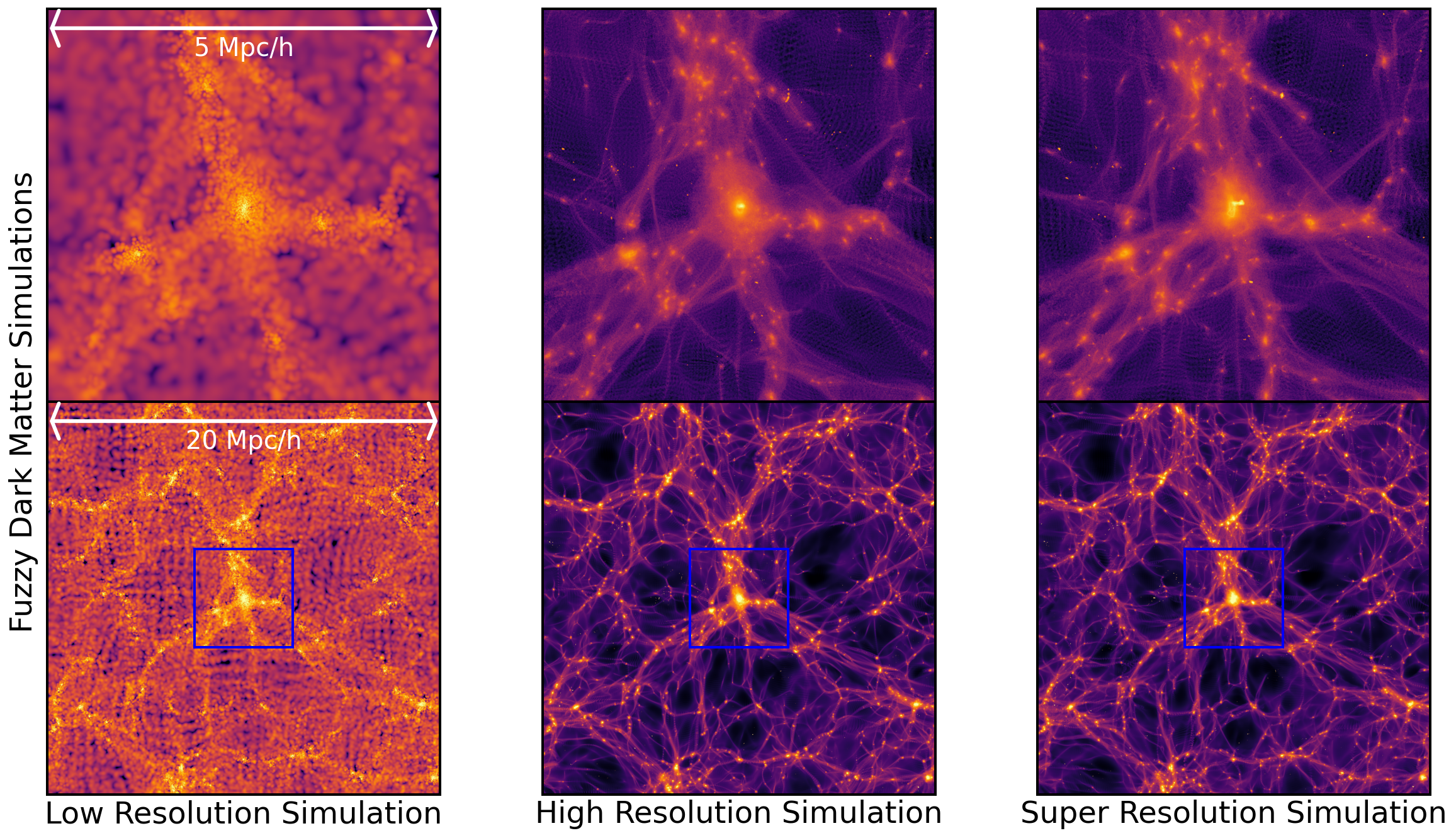
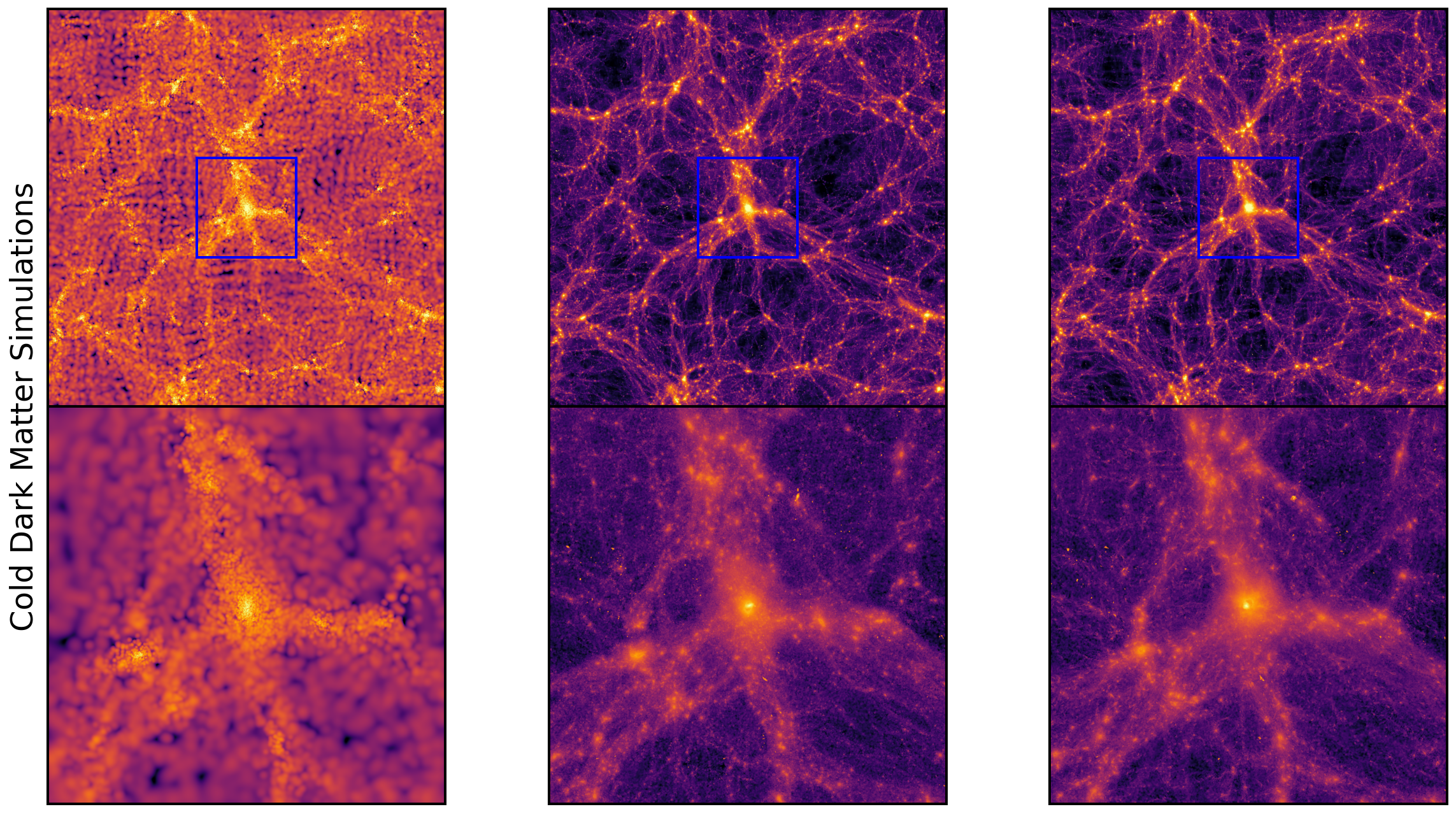
Figure 1: 2D visualization of the LR, HR, and SR density distributions for both FDM and LCDM. The central rows show a slice of the enter 20 Mpc simulations, while the top and bottom rows show zoomed in portions of those simulations. The zoomed in locations are indicated with the blue boxes on the central panels. The upper half of the figure is showing the Fuzzy Dark Matter simulations, while the lower half is showing the Cold Dark Matter simulations.

2 Methods

2.1 Data

We work with N-body simulation data for the FDM and LCDM models. Both sets are run with initial conditions consistent with the WMAP9 cosmology with matter density $\Omega_{\rm m}=0.2814$, dark energy density $\Omega_{\Lambda}=0.7186$, baryon density $\Omega_{\rm b}=0.0464$, power spectrum normalization $\sigma_{8}=0.82$, spectral index $n_{s}=0.971$, and Hubble parameter $h=0.697$. The difference between them is solely encoded in the initial power spectrum, with the largest difference being on small scales. Our FDM simulations employ the initial power spectrum at $z=99$ generated by AXIONCAMB (Hlozek et al. 2015), also used in N19. The FDM particle mass assumed in our models is $2.5\times 10^{-22}$ eV, which leads to a damping scale relative to LCDM in the linear P(k) at $k=18\;h\;{\rm Mpc}^{-1}$ (see Figure 2 of N19).

We use the current version of the MP-GADGET cosmological N-body code (Bird et al. 2022, part of the GADGET code family [Springel 2005]) to evolve the initial conditions forward in time. The simulation is run in dark matter only mode, with particle mass $4.6\times 10^{6}\,M_{\odot}$, and a cubical periodic volume of side length $20h^{-1}{\rm Mpc}$. The simulation is evolved from redshift $z=99$ to $z=2$, and we use the final, $z=2$ snapshot exclusively in our study. We do this because at high redshifts the differences between the evolved density distributions in FDM and LCDM have not been erased by non-linear evolution (see e.g., Iršič et al. 2017b, N19). Sixteen simulation realizations with different random seeds are run for each of the FDM and LCDM models. Each of these realizations consists of an LR and and HR pair. The mass per particle of the LR simulation is 512 times less than for HR, i.e., $2.4\times 10^{9}\,M_{\odot}$.

2.2 Deep Learning Models

GANs (Goodfellow et al. 2014) are a deep learning technique that consists of two separate neural networks, named the generative and the discriminative network. The generative network generates candidate distributions, and the discriminative network tries to determine if that distribution came from an HR simulation (in our case), or from the generator. In doing this, the GAN learns to generate new data with characteristics matching the training set. We use a Conditional GAN (CGAN), where the input to the generator is both noise and a low resolution (LR) version of the simulation data. The process adds noise during convolution to add irregularity to the smaller scales that was previously absent. These irregularities become small-scale over and under densities in the distribution of particles of the resulting super-resolution (SR) simulation.

The specific neural network architecture used is that described fully in Ni et al. (2021) and the reader is referred to that paper for more details. Briefly, the resolution enhancement is applied to the particle distribution, through the displacement field (displacement of particles from their initial positions). The particle displacements and their velocities in a low resolution simulation and a noise vector are the inputs to the generator. The discriminator network receives the high resolution particle positions and displacements, as well as an Eulerian density field representing those particles assigned to grid cells using a Cloud-in-Cell scheme. The loss function is the total distance between the real and generated datasets using optimal transport, also known as the Wasserstein distance, meaning that the type of GAN we use is a Wasserstein GAN (WGAN, see Gulrajani et al. 2017 for the particular variant we use). This GAN variation is more stable and requires less tuning than the original GAN.

2.3 Training

We focus on training our GAN to generate FDM SR particle distributions from LR distributions. We do this to determine how well a GAN can create a valid SR particle distribution for FDM. When passing the simulation data to the network for training, we first split it into discrete chunks, due to GPU memory limitations. The chunks have a side length one fifth of the simulation volume, and the LR simulation input includes an extra margin of the same size, making use of the periodic boundary conditions of the simulation.

After the network is fully trained, we generate three different types of SR distributions; one of LCDM from a LR LCDM distribution, one of FDM from a LR FDM distribution and one of FDM from a LR LCDM distribution. The LCDM to LCDM SR process follows that employed by Ni et al. (2021), except that it extends to spatial scales 5 times smaller and a mass resolution 125 times greater. This LCDM SR model is used as a baseline for determining the success of the FDM GAN training, as well as a test of the SR procedure on smaller scales than have yet been tested. The reader is referred to Section 2.3 of Ni et al. (2021) for more details.

The FDM to FDM SR distribution was our test case and the LCDM to FDM was used as a proof of concept for seeing if our FDM training could generate an FDM output from an LCDM input. During training we analysed all of the SR distributions by visual observation and by use of the density field power spectrum, P(k), which is used as a metric to evaluate the SR distribution fidelity. We focus in particular on the region between $k=20\;h\;{\rm Mpc}^{-1}$ and $k=150\;h\;{\rm Mpc}^{-1}$ as it shows how much small scale structure the SR process has added from the original LR distribution.

3 Results

3.1 Visual impression

Fig. 1 shows slices of the dark matter density distributions for both LCDM and FDM at all resolutions. We show both a slice through the whole box as well as a smaller region centered on the most massive halo in the volume. Visually the HR and SR distributions for FDM tend to display less small scale structure as indicated by fewer smaller clumps of particles than the distributions for LCDM as expected from the different models. The LR simulations for both FDM and LCDM are very similar in appearance however, and we shall see in Section 3.2 that the most of the extra fluctuation power in LCDM with respect to FDM is below the Nyquist frequency of the LR model. Comparing the HR and SR distributions for both models, we have difficulty telling them apart in general appearance, although individual small scale clumps are different, when looked at closely. As the SR and HR models should only be statistically similar, this is to be expected.

If we look at filaments in the FDM model (for example on the right hand side of the close up panel), we can see that that they are broken up into regularly spaced clumps, like beads on a string. These small halos are unphysical, as has been noted in the context of other cosmological models by authors from Melott & Shandarin (1989) onwards (including most extensively by Wang & White 2007 and Angulo et al. 2013). These occur most prominently when a model has little power at frequencies close to the Nyquist frequency of the initial particle grid. If the initial particle distribution is indeed set up in a grid fashion, these fake halos will remain. They are also exacerbated when the numerical resolution is significantly smaller than the grid spacing (see e.g., Splinter et al. 1998), as is usual in cosmological simulations. We will see in Section 3.3 when we examine the halo mass function that they are found by the halo finder, and dominate the number of halos below a certain mass. This issue has lead some papers (e.g., N19) to not use halos below a certain mass in their analyses, using the empirically determined halo mass limit for spurious fragmentation of Wang & White (2007). In our case, we note that the SR FDM simulation is sufficiently similar to the HR model that it also includes these spurious objects.

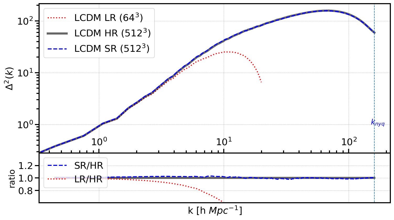
(a) LCDM

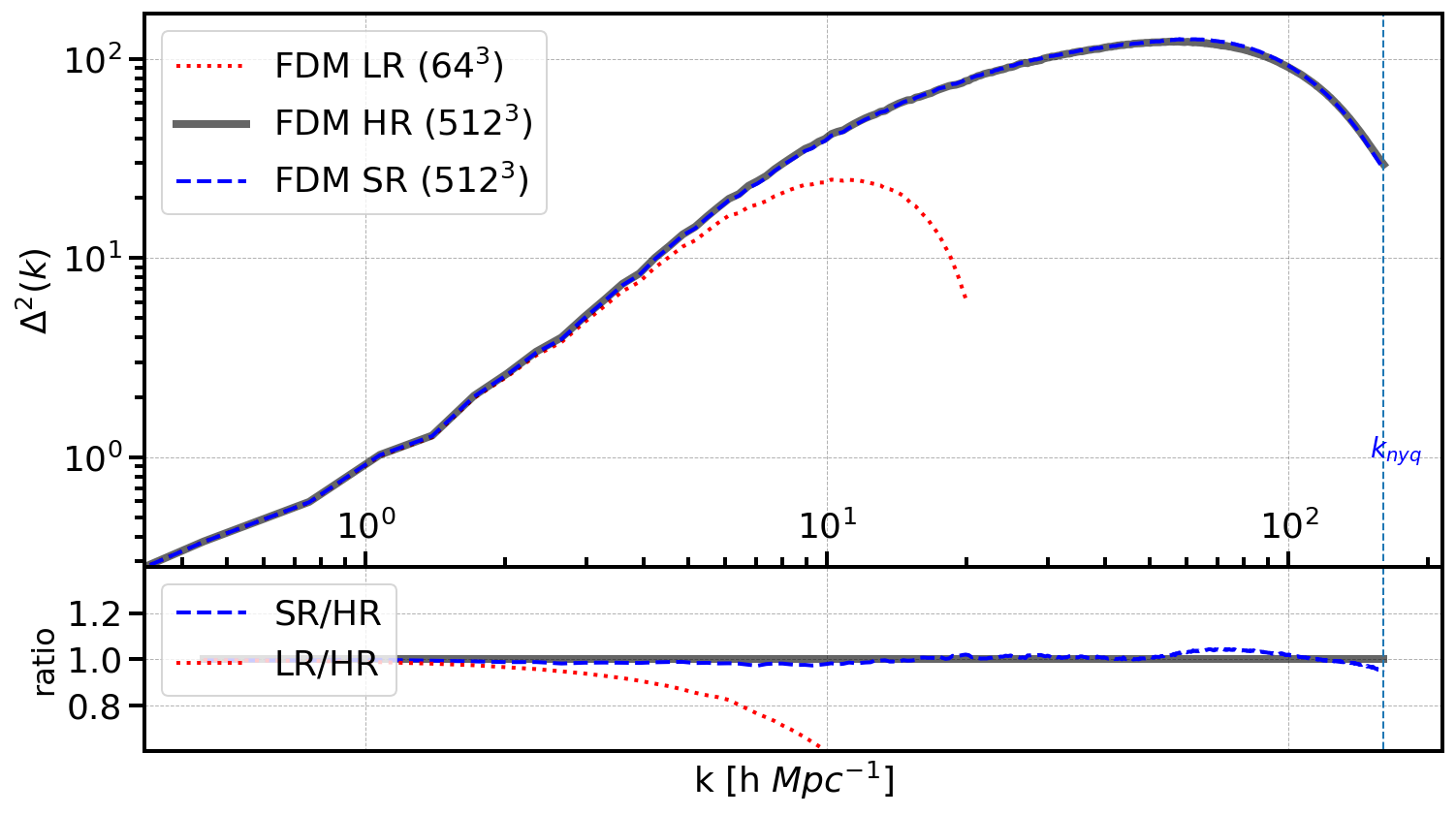
(b) FDM

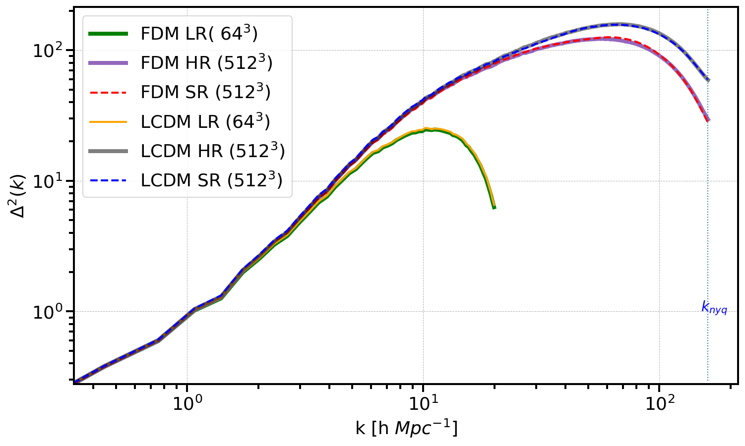
(c) Combined

Figure 2: The power spectra for both LCDM and FDM. (a) gives the LCDM dimensionless matter power spectrum $\Delta^{2}$ computed for LR (dotted red), HR (black), and SR (dashed blue). The bottom panel gives the ratio of of both LR (dotted red) and SR (dashed blue) to HR (b) displays the same for FDM. (c) displays all power spectra for both LCDM and FDM on a combined plot. The dashed black line on the right of the figure marks the Nyquist frequency.

3.2 Power spectrum

We compute the power spectra, $P(k)$ for all simulations after assigning the particles to a grid with the same dimensions as the intial particle grid. In Fig. 2, the dimensionless power spectra ($\delta^{2}(k)=k^{3}P(k)$ for both dark matter models are shown, with all results being at our chosen redshift of $z=2$. We plot all curves up to the Nyquist frequency of the grid, including for the LR simulations, for which this is a factor of 8 lower than for HR and SR. The LCDM model at this redshift has more power on small scales than FDM, 50% less at the Nyquist frequency, the smallest scale plotted. The SR power spectrum matches the HR spectrum within 5% on all scales for both FDM and LCDM indicating the GAN was successfully trained.

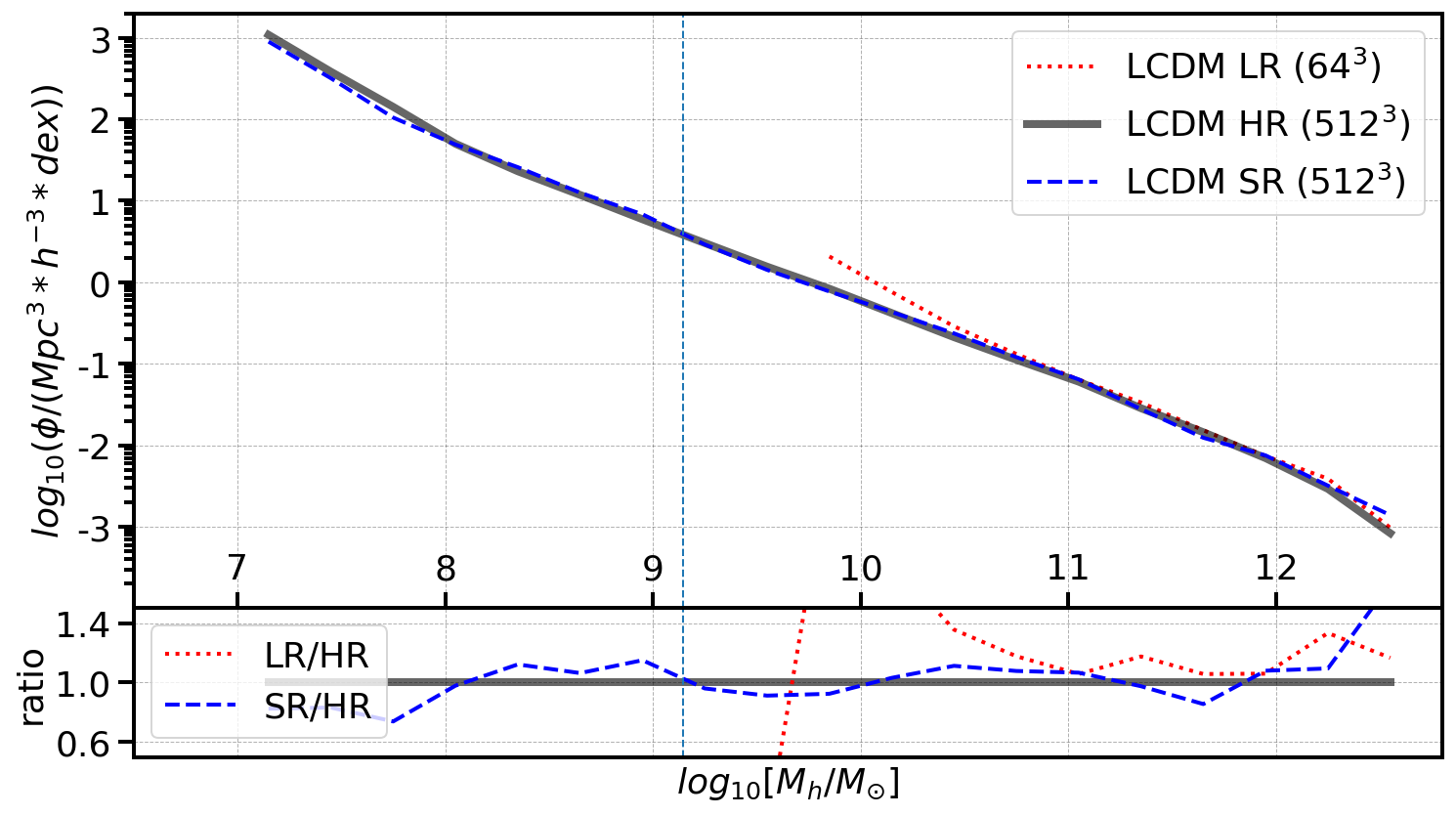
(a) LCDM

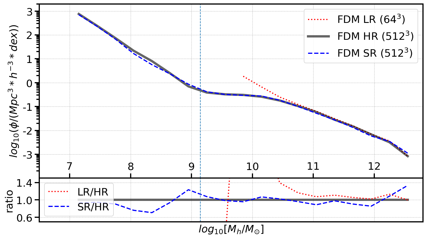
(b) FDM

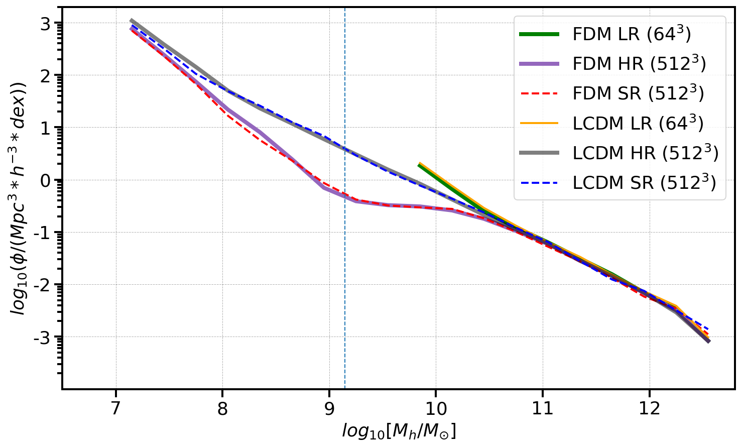
(c) Combined

Figure 3: The halo mass functions for LCDM and FDM. (a) gives the LCDM halo mass functions of the LR (dotted red), HR (black) and SR (dashed blue). The bottom panel gives the ratios of LR (dotted red) and SR (dashed blue) to HR. (b) displays the same for FDM. (c) displays all mass functions for both LCDM and FDM on a combined plot. The vertical dashed grey line indicates the 300 particle cutoff for halo size.

3.3 Halo mass function

We make halo catalogues from the simulation output, using a Friend-of-Friends halo finder (Davis et al. 1985), with a linking length of 0.2 times the mean interparticle separation. Following N19 we choose 300 particles as the cutoff below which halos are not simulated reliably. Numerical artefacts strongly affect the small halo mass function in models with low power on halo scales as mentioned in Section 3.1 above.

In Figure 3, we show the halo mass functions are given for both LCDM and FDM. We can see that the SR and HR mass functions match within 5% for both FDM and LCDM. Near the 300 particle cutoff, which corresponds to halo masses of $1.4\times 10^{9}\,M_{\odot}$, we can see that the HR and SR mass functions for FDM are less than those of LCDM by an order of magnitude. This corresponds to a deficit of low mass galaxies with respect to LCDM which could be used to constrain the FDM particle mass (e.g., N19). At redshift $z=2$ which we are plotting here, the deficit is smaller than at higher redshifts, but still substantial for the relatively low FDM mass we are simulating ($2.5\times 10^{-22}$ eV).

We plot halos down to 2 particles, a mass of $9\times 10^{6}\,M_{\odot}$ (for HR and SR). Even though most of the halos below 300 particles are not reliably simulated halos, due to both numerical problems with FDM/WDM (as mentioned above) and shot noise, we can see that both the SR and HR simulation results track each other closely all the way down to the lowest masses plotted. Because the SR simulation process works with the particle displacements and velocities it effectively generates simulation data in all its details, including the spurious halos that were present in the training set.

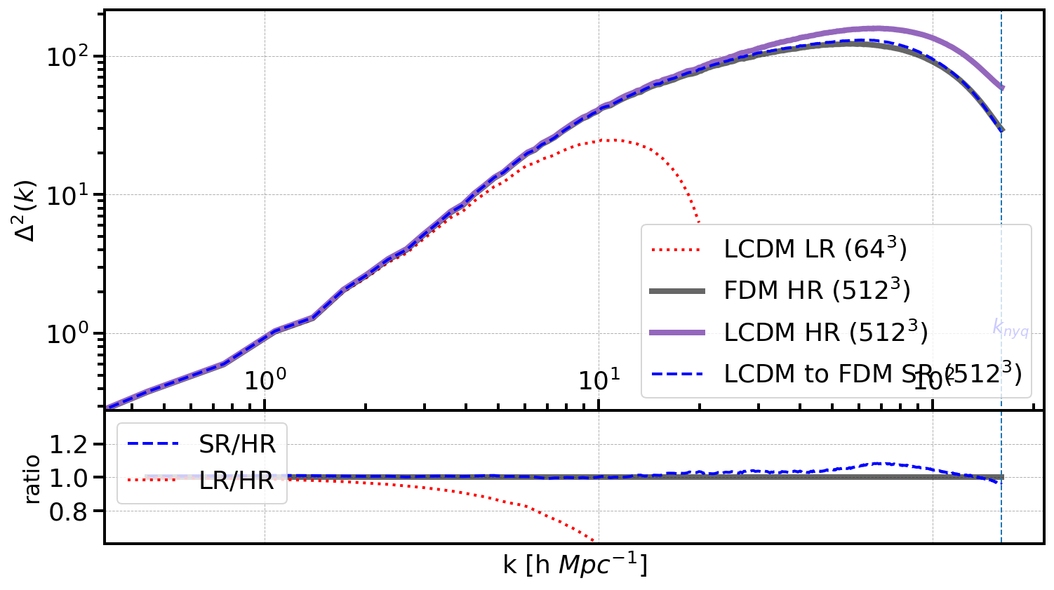
(a) Power Spectrum

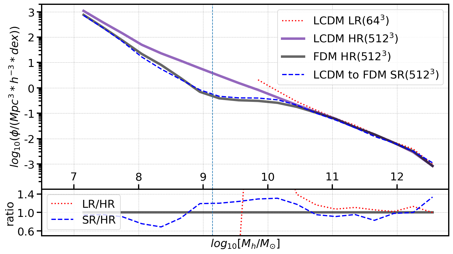
(b) Halo Mass Function

Figure 4: Summary statistics for an FDM SR simulation using LR from a different model (LCDM) as an input (see Section 3.4). (a) P(k) for the different models, as in Figure 2, with the FDM HR using an LCDM LR input shown as a dashed line. (b) The halo mass functions for the different models, as in Figure 3.

3.4 SR of FDM using LCDM LR

The LCDM and FDM simulations have very similiar initial (linear) power spectra at scales larger than the damping scale ($k=18\;h\;{\rm Mpc}^{-1}$ in the case of $m_{\rm FDM}=2.5\times 10^{-22}$ eV, see Figure 2 of N19.). This scale is above the Nyquist frequency of the LR simulations, and so opens the possibility of using LR simulations to make SR simulations for a different model. In our final test we have tried using the LR LCDM simulations as an input to the FDM-trained network. The results are shown in Figure 4(a), where we can see that the resulting SR FDM power spectrum is quite close to that of the HR FDM model, with a maximum deviation of 8%. The halo mass function, in Figure 4(b) is also within 20% of the FDM HR results.

These tests show that we could in principle use the same LR simulations to generate different SR dark matter models, as long as the differences in the power spectra are on small enough scales and the accuracy is sufficient for the desired use case (e.g., mock catalogues). The NNs in the present case are trained on a specific DM model, however, and so require full HR simulations of that a model. A more general tool would be able to train on a range of models and interpolate between them. The NN architecture StyleGAN2 (e.g., Karras et al. 2019) has shown some promise for field level emulation in different cosmological models (see e.g., Jamieson et al. 2022) and we hope to explore its use in super-resolution in future work.

4 Summary and Discussion

4.1 Summary

This work attempts to extend the use case of the super resolution architecture developed in Li et al. (2021) beyond the LCDM model. The results indicate this extension works well for the case of FDM. Other viable alternative DM models, such as self-interactive DM (Vogelsberger et al., 2012) or warm dark matter (Bode et al., 2001) also feature suppression of the linear matter power spectrum. Extensions like this indicate that the approach is ripe for further development to allow a single trained network to be able to produce simulations with different cosmological models, which would be an extremely useful tool in studying possible alternate cosmological models.

4.2 Discussion

This paper represents a small step on the way to the exploitation of AISR techniques in cosmology. We have shown that dwarf galaxies and subhalos with masses of $10^{9}\,M_{\odot}$ can be quite accurately simulated, even for the LCDM model, which has significant small scale structure, with orbit crossing and virialization obviously being very important on these scales. The models still only include dark matter, and the real test will come when methods to include hydrodynamics are developed. Hydrodynamics will also break the approximate scale invariance of the LCDM model on these scales and provide an even more strenuous test of the AISR technique.

An application of FDM simulations is to compare to the abundance and statistical properties of galaxies and therefore constrain the FDM particle mass. At present some of the tightest constraints on this parameter come from measurements of the Lyman-alpha forest power spectrum (e.g., Iršič et al. (2017a). N19 have shown that the high redshift galaxy population can also provide competitive constraints, and with different possible systematic errors (for example the Lyman-$\alpha$ forest is also sensitive to the temperature of the intergalactic medium). In this paper we have used simulations at the relatively high redshift of $z=2$ because non-linear evolution to lower redshifts tends to erase the differences between CDM and FDM. At higher redshifts relevant for JWST observations (e.g., $z=7-12$, Marshall et al. 2022, Bradley et al. 2022), N19 have shown using hydrodynamic simulations that there are significant differences in the galaxy stellar mass functions between an FDM and LCDM models. In our simulations, the maximum $\sim$ 5% differences between HR and SR are smaller than those between LCDM and FDM models with mass of $2.5\times 10^{-22}$ eV. As shown by Li et al. (2021), the accuracy of SR increases at higher redshift, meaning that heavier mass FDM models will be feasible to simulate with FDM.

Ideal applications for the AISR techniques will be studies of observational systematics using large mocks, where the uncertainties modelled are larger than the demonstrated accuracy of AISR. In a similar vein, semi-analytic models could be run on AISR FDM simulations, where the uncertainties in the model parameters are larger than AISR accuracy. The speed of AISR would allow many tens of thousands mock catalogs to be generated for the same computational cost of a single HR model. We have also shown that for models such as CDM where the large-scale P(k) is close to that of FDM, it is even possible to use the same LR simulation to make SR models with different particle masses, thereby saving on the cost of running the larger LR N-body simulation.

Because we have used a very simplified treatment of FDM, the truncation of the input power spectrum, our conclusions about the success of AISR also apply to other models when this approximation to the small scale behaviour is used, such as WDM. There is however nothing in principle to prevent the use of AI SR techniques together with more physically accurate methods for simulating structure formation in these models. The methods used by e.g., Mocz et al. (2017) and May & Springel (2021) to solve the Schrodinger-Poisson equation could be used to train the NN used in AISR. This could be used to produce rapid simulations that reproduce the quantum pressure effects seen by e.g., May & Springel (2022) beyond those linked directly to the suppression of power. We note that particle discreteness problems that cause fake substructures to form in models with low small scale power are also present in our current AIRS model results (and are visible in Figures 1). These could be corrected with better training simulations and analysis (e.g., Angulo et al. 2013, May & Springel 2021).

Data Availability

The SR models and the pipeline used to generate the SR fields are available at https://github.com/yueyingn/SRS-map2map. The simulation outputs and measured summary statistics are available on request from the authors.

References

- Angulo et al. (2013) Angulo R. E., Hahn O., Abel T., 2013, MNRAS, 434, 3337
- Arbey & Mahmoudi (2021) Arbey A., Mahmoudi F., 2021, Progress in Particle and Nuclear Physics, 119, 103865
- Bird et al. (2022) Bird S., Ni Y., Di Matteo T., Croft R., Feng Y., Chen N., 2022, MNRAS, 512, 3703
- Bode et al. (2001) Bode P., Ostriker J. P., Turok N., 2001, ApJ, 556, 93
- Bode et al. (2019) Bode M., Gauding M., Lian Z., Denker D., Davidovic M., Kleinheinz K., Jitsev J., Pitsch H., 2019, Using Physics-Informed Super-Resolution Generative Adversarial Networks for Subgrid Modeling in Turbulent Reactive Flows, doi:10.48550/ARXIV.1911.11380, %****␣FDMSR.bbl␣Line␣50␣****https://arxiv.org/abs/1911.11380
- Bond et al. (1980) Bond J. R., Efstathiou G., Silk J., 1980, Phys. Rev. Lett., 45, 1980
- Bradley et al. (2022) Bradley L. D., et al., 2022, arXiv e-prints, p. arXiv:2210.01777
- Colombi et al. (1996) Colombi S., Dodelson S., Widrow L. M., 1996, ApJ, 458, 1
- Davis et al. (1985) Davis M., Efstathiou G., Frenk C. S., White S. D. M., 1985, ApJ, 292, 371
- Del Popolo & Le Delliou (2017) Del Popolo A., Le Delliou M., 2017, Galaxies, 5, 17
- Goodfellow et al. (2014) Goodfellow I., Pouget-Abadie J., Mirza M., Xu B., Warde-Farley D., Ozair S., Courville A., Bengio Y., 2014, in Advances in neural information processing systems. pp 2672–2680
- Goodfellow et al. (2016) Goodfellow I. J., Bengio Y., Courville A., 2016, Deep Learning. MIT Press, Cambridge, MA, USA
- Gulrajani et al. (2017) Gulrajani I., Ahmed F., Arjovsky M., Dumoulin V., Courville A., 2017, arXiv e-prints, p. arXiv:1704.00028
- Hlozek et al. (2015) Hlozek R., Grin D., Marsh D. J. E., Ferreira P. G., 2015, Phys. Rev. D, 91, 103512
- Hu et al. (2000) Hu W., Barkana R., Gruzinov A., 2000, Phys. Rev. Lett., 85, 1158
- Hui et al. (2017) Hui L., Ostriker J. P., Tremaine S., Witten E., 2017, Phys. Rev. D, 95, 043541
- Iršič et al. (2017a) Iršič V., et al., 2017a, Phys. Rev. D, 96, 023522
- Iršič et al. (2017b) Iršič V., Viel M., Haehnelt M. G., Bolton J. S., Becker G. D., 2017b, Phys. Rev. Lett., 119, 031302
- Jamieson et al. (2022) Jamieson D., Li Y., Alves de Oliveira R., Villaescusa-Navarro F., Ho S., Spergel D. N., 2022, arXiv e-prints, p. arXiv:2206.04594
- Jiang et al. (2020) Jiang C. M., et al., 2020, CoRR, abs/2005.01463
- Kamionkowski & Liddle (2000) Kamionkowski M., Liddle A. R., 2000, Phys. Rev. Lett., 84, 4525
- Karras et al. (2019) Karras T., Laine S., Aittala M., Hellsten J., Lehtinen J., Aila T., 2019, Analyzing and Improving the Image Quality of StyleGAN, doi:10.48550/ARXIV.1912.04958, https://arxiv.org/abs/1912.04958
- Kodi Ramanah et al. (2020) Kodi Ramanah D., Charnock T., Villaescusa-Navarro F., Wandelt B. D., 2020, MNRAS, 495, 4227
- Lakshminarayanan et al. (2012) Lakshminarayanan V., Calvo M., T.Alieyva eds, 2012, Mathematical Optics Classical,Quantum and Computational Methods. CRC Press
- Li et al. (2021) Li Y., Ni Y., Croft R. A. C., Di Matteo T., Bird S., Feng Y., 2021, Proceedings of the National Academy of Science, 118, e2022038118
- Marshall et al. (2022) Marshall M. A., et al., 2022, MNRAS, 516, 1047
- May & Springel (2021) May S., Springel V., 2021, MNRAS, 506, 2603
- May & Springel (2022) May S., Springel V., 2022, arXiv e-prints, p. arXiv:2209.14886
- Melott & Shandarin (1989) Melott A. L., Shandarin S. F., 1989, ApJ, 343, 26
- Mocz et al. (2017) Mocz P., Vogelsberger M., Robles V. H., Zavala J., Boylan-Kolchin M., Fialkov A., Hernquist L., 2017, MNRAS, 471, 4559
- Mocz et al. (2018) Mocz P., Lancaster L., Fialkov A., Becerra F., Chavanis P.-H., 2018, Phys. Rev. D, 97, 083519
- Ni et al. (2019) Ni Y., Wang M.-Y., Feng Y., Di Matteo T., 2019, MNRAS, 488, 5551
- Ni et al. (2021) Ni Y., Li Y., Lachance P., Croft R. A. C., Matteo T. D., Bird S., Feng Y., 2021, Monthly Notices of the Royal Astronomical Society, 507, 1021
- Niemeyer (2020) Niemeyer J. C., 2020, Progress in Particle and Nuclear Physics, 113, 103787
- Paduroiu (2022) Paduroiu S., 2022, Universe, 8, 76
- Russell & Norvig (2020) Russell S. J., Norvig P., 2020, Artificial Intelligence: a modern approach, 4 edn. Pearson
- Schwabe & Niemeyer (2022) Schwabe B., Niemeyer J. C., 2022, Phys. Rev. Lett., 128, 181301
- Smith & Markovic (2011) Smith R. E., Markovic K., 2011, Phys. Rev. D, 84, 063507
- Spergel & Steinhardt (2000) Spergel D. N., Steinhardt P. J., 2000, Phys. Rev. Lett., 84, 3760
- Splinter et al. (1998) Splinter R. J., Melott A. L., Shandarin S. F., Suto Y., 1998, ApJ, 497, 38
- Springel (2005) Springel V., 2005, MNRAS, 364, 1105
- Tulin & Yu (2018) Tulin S., Yu H.-B., 2018, Phys. Rep., 730, 1
- Vogelsberger et al. (2012) Vogelsberger M., Zavala J., Loeb A., 2012, MNRAS, 423, 3740
- Vogelsberger et al. (2020) Vogelsberger M., Marinacci F., Torrey P., Puchwein E., 2020, Nature Reviews Physics, 2, 42
- Wang & White (2007) Wang J., White S. D. M., 2007, MNRAS, 380, 93
- Wang et al. (2019) Wang Z., Chen J., Hoi S. C. H., 2019, arXiv e-prints, p. arXiv:1902.06068
- Weinberg et al. (2015) Weinberg D. H., Bullock J. S., Governato F., Kuzio de Naray R., Peter A. H. G., 2015, Proceedings of the National Academy of Science, 112, 12249
- Werhahn et al. (2019) Werhahn M., Xie Y., Chu M., Thuerey N., 2019, CoRR, abs/1906.01689
- White & Croft (2000) White M., Croft R. A. C., 2000, ApJ, 539, 497