Periodic analogues of the Kerr solutions:
a numerical study

Abstract

In recent years black hole configurations with non standard topology or with non-standard asymptotic have gained considerable attention. In this article we carry out numerical investigations aimed to find periodic coaxial configurations of co-rotating 3+1 vacuum black holes, for which existence and uniqueness has not yet been theoretically proven. The aimed configurations would extend Myers/Korotkin-Nicolai’s family of non-rotating (static) coaxial arrays of black holes. We find that numerical solutions with a given value for the area $A$ and for the angular momentum $J$ of the horizons appear to exist only when the separation between consecutive horizons is larger than a certain critical value that depends only on $A$ and $|J|$. We also establish that the solutions have the same Lewis’s cylindrical asymptotic as Stockum’s infinite rotating cylinders. Below the mentioned critical value the rotational energy appears to be too big to sustain a global equilibrium and a singularity shows up at a finite distance from the bulk. This phenomenon is a relative of Stockum’s asymptotic’s collapse, manifesting when the angular momentum (per unit of axial length) reaches a critical value compared to the mass (per unit of axial length), and that results from a transition in the Lewis’s class of the cylindrical exterior solution. This remarkable phenomenon seems to be unexplored in the context of coaxial arrays of black holes. Ergospheres and other global properties are also presented in detail.

1 Introduction

In recent years vacuum black hole configurations with non standard topology or with non-standard asymptotic have gained considerable attention. In five dimensions, Emparan and Reall [1] have found asymptotically flat stationary solutions with ring-like $S^{1}\times S^{2}$ horizon and Elvang and Figueras [2] have found asymptotically flat black Saturns, where a black ring $S^{1}\times S^{2}$ rotates around a black sphere $S^{3}$. More recently Khuri, Weinstein and Yamada [3, 4], have found periodic static coaxial arrays of horizons either with spherical $S^{3}$ or ring-like $S^{1}\times S^{2}$ topology. Rather than asymptotically flat, these latter configurations have Levi-Civita/Kasner asymptotic and generalize to five dimensions the important Myers/Korotkin-Nicolai (MKN) family of vacuum static $3+1$ solutions [5, 6, 7], referred sometimes as “periodic Schwarzschild”, as their are obtained as “linear” superpositions of Schwarzschild’s solutions via Weyl’s method. The search for new solutions has branched rapidly to higher dimensions and to different fields, giving by now a rich landscape of topologies, [8]. However, the question whether “periodic Kerr” configurations generalizing the “periodic Schwarzschild” exist, either in four or higher dimensions, remains still open. In this article we aim to investigate this latter problem in four dimensions numerically. Specifically, we carry out numerical investigations pointing at constructing periodic coaxial configurations of co-rotating $3+1$ black holes.

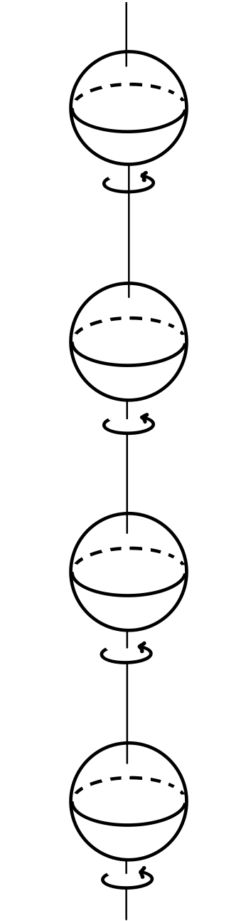
Figure 1: Periodic configuration of co-rotating coaxial black holes. The horizons are equally spaced, have the same area $A$ and angular momentum $J$.

The equally spaced horizons are all intended to have the same area $A$, angular momentum $J$ and angular velocity $\Omega_{H}$, (see Figure 1). This problem has been discussed by Korotkin and Nicolai in [7] (section 4) and also by Mavrin in [9], however non conclusively. Numerical investigations and an analysis of the solution space and of the global properties of the solutions appear to be carried out here for the first time.

This problem poses a number of difficulties on the numerical side. The central, relevant equation to solve is an harmonic map in two dimensions, whose solutions are found as the stationary regime of a heat-type flow for the harmonic map. The numerical study of the problem allowed us to find the correct formulation of the asymptotic boundary conditions, which constituted the main difficulty of the problem.

The results of this paper can be summarized as follows. Periodic configurations having a given value of $J$ and $A(>8\pi|J|)$, appear to exist only when the separation between the horizons is larger than a certain critical value that depends only on $A$ and $|J|$. The smaller the separation the bigger the angular velocity $|\Omega_{H}|$ and the bigger the rotational energy and the total energy. The asymptotic (suitably defined) matches always a Lewis’s solution [10] as in the Stockum’s rotating cylinders [11]. Furthermore, as the separation between horizons gets smaller than the critical value, no asymptotic can hold the given amount of energy and we evidence a singularity formation at a finite distance from the bulk. Roughly speaking, the asymptotic “closes up” due to too much rotational energy. This phenomenon is similar to Stockum’s asymptotic collapse, studied in [11], and manifesting when the angular momentum (per unit of axial length) increases past a critical value compared to the mass (per unit of axial length). When the rotation increases, the exterior Lewis solution transits from one extending to infinity to one blowing up at a finite distance from the material cylinder. There is a change in the Lewis’s class. This change of class, that prevents black holes from getting too close, appears to be entirely novel in our context and is in sharp contrast to what occurs for the periodic Schwarzschild configurations, where horizons can get arbitrarily near. The ergo-regions are always bounded and disjoint. We observe though that below the critical separation the ergospheres can indeed merge, but such solutions do not extend to infinity. The Komar mass $M$ per black hole satisfies the relevant inequality,

$$\sqrt{\frac{A}{16\pi}+\frac{4\pi J^{2}}{A}}\leq M,$$ (1)

and equality is approached as the separation between the black holes grows unboundedly and the geometry near the horizons approaches that of Kerr.

The paper is organized as follows. In section 2 we overview the theoretical and numerical problem commenting on the difficulties and strategies. We present the main equations to be solved and recall the Lewis’s classes. We also discuss the boundary condition for the harmonic map heat flow and give the precise set up for the numerical study. In section 3 we discuss the numerical techniques used to solve the equations. In section 4 we present our results, discussing several features of the numerical solutions obtained, and in section 5 we contextualize our work and give some possible future directions to our study.

2 The setup

2.1 Overview of the mathematical and numerical problem

The configurations that we are looking for have three degrees of freedom that we will take to be the area $A$, the angular momentum $J$, and the period $L$, with $L$ linked to the physical separation between consecutive black holes. These parameters need to be incorporated into the boundary conditions of the main equations. The stationary and axisymmetric metrics are assumed to be in Weyl-Papapetrou form and are recalled in (2), (see for instance [12]). In this expression $\rho\in\mathbb{R}^{+}$ and $z\in\mathbb{R}$ are the Weyl-Papapetrou cylindrical coordinates and play a role in what follow. For Weyl-Papapetrou metrics, the Einstein equations reduce to find an axisymmetric harmonic map $(\omega(\rho,z),\eta(\rho,z)):\mathbb{R}^{3}\rightarrow\mathbb{H}^{2}$ from $\mathbb{R}^{3}$ into the hyperbolic space $\mathbb{H}^{2}$. Here $\eta$ is the norm squared of the axisymmetric Killing field and $\omega$ is the twist potential. All the metric components can be recovered from $\eta$ and $\omega$ after line-integrations. The full set of reduced equations are presented in section 2.2. The harmonic map equations are (3)-(4) and the metric components are (5) after the line integrations of (6) and (7).

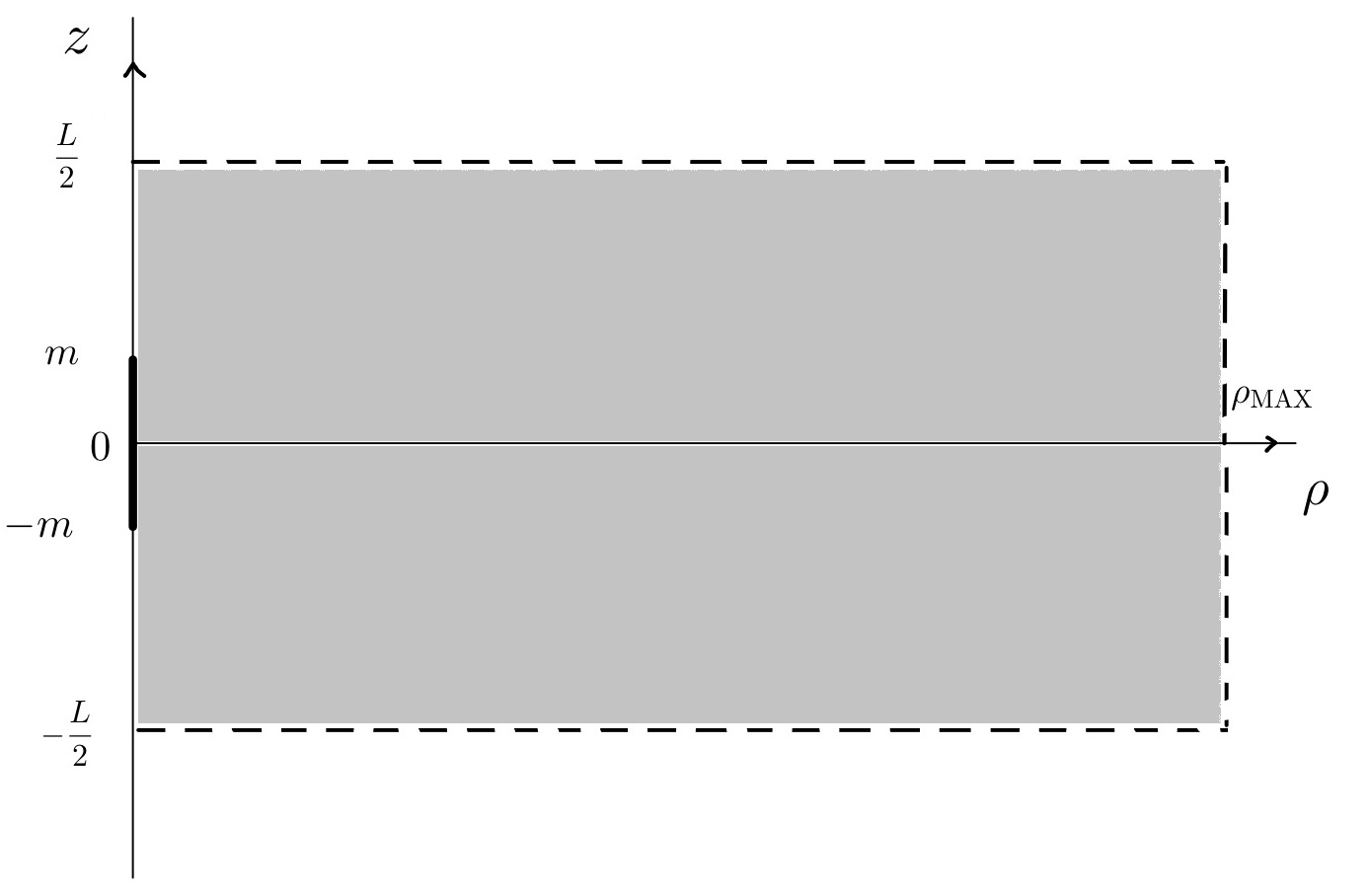
Figure 2: The numerical domain with the horizon marked as a thick interval.

As we look for metrics periodic in $z$, we restrict the analysis to the region $\{\rho\geq 0,-L/2\leq z\leq L/2\}$ keeping appropriate periodicity conditions on the top and bottom lines $\{\rho\geq 0,\ z=\pm L/2\}$. Here $L$ is the period mentioned earlier and is a free parameter. The harmonic map equations for $\omega$ and $\eta$ need to be supplied with boundary data on the border $\{\rho=0,-L/2\leq z\leq L/2\}$. This boundary contains the horizon $\mathcal{H}=\{\rho=0,\ -m\leq z\leq m\}$, and the two components of the axis ${\mathcal{A}}$ which is the complement of $\mathcal{H}$. The boundary conditions arise from two sides: from the natural conditions that $\eta$ and $\omega$ must verify on horizons and axes, and from fixing the values of the area $A$ and of the angular momentum $J$. The angular momentum $J$ is set by specifying Dirichlet data for $\omega$ on the axis, whereas the area $A$ is set by specifying the limit values of $\eta/\rho^{2}$ at the poles $z=\pm m$. The fact that one can incorporate $A$ and $J$ into the boundary conditions in this simple way is a great advantage of the formulation. The parameter $m$ that may seem to be a free parameter, is equal to the surface gravity $\kappa$, ($\kappa^{2}:=-\langle\nabla\partial_{t},\nabla\partial_{t}\rangle/2$), of the horizons times $A/4\pi$ and therefore can be fixed using the freedom in the definition of the stationary Killing field $\partial_{t}$, or the definition of time in (2). In this article we chose $\kappa=\kappa(A,J)$ equal to the surface gravity of the Kerr black holes for the given $A$ and $J$.

The full set of boundary conditions on $\{\rho=0,-L/2\leq z\leq L/2\}$ is discussed in section 2.4.

In practice, the harmonic map equations need to be solved numerically on a finite rectangle $[0,\rho_{\rm\small{MAX}}]\times[-L/2,L/2]$, and this adds the extra difficulty of finding natural boundary conditions also at $\rho=\rho_{\rm MAX}$, for $\omega$ and for $\eta$. On physical grounds one expects the solutions to become asymptotically independent of $z$ and indeed approaching the Lewis models of Stockum’s rotating cylinders that we recall in section 2.3. But the problem is that one does not know a priori which Lewis solution shows up for the given $A$, $J$ and $L$. If that information were known, then one could easily supply appropriate boundary conditions at $\rho_{\rm MAX}$. Now, all Lewis solutions have $\omega=wz$, so we make $\omega(\rho_{\rm MAX},z)=wz$. For $\eta$ however not such single choice is possible. We set a Neumann type of boundary condition for $\eta$ and for that we use that, on actual solutions, the Komar mass expression $M(\rho)$, in (34), is constant, so that $M(\rho_{\rm MAX})=M(\rho)$ easily relates $\partial_{\rho}\eta(\rho_{\rm MAX})$ to $\eta$ and $\omega$ at any $\rho<\rho_{\rm MAX}$. Then, to define the condition for $\eta$ we make use of this relation, equating $\partial_{\rho}\eta(\rho_{\rm MAX})$ to the average of the Komar mass expression in the bulk $0<\rho<\rho_{\rm MAX}$. We discuss this condition in section 2.4, and state it in (34). This peculiar Neumann condition for $\eta$ at $\rho_{\rm MAX}$ is what gave us the best numerical results in terms of the speed and the stability of our code.

To find solutions for the harmonic map system, we run a harmonic map heat flow with certain initial data, and look for the stationary solutions in the long time. We can show that the numerical solutions for two different values of $\rho$, say $1\ll\rho_{\rm MAX}^{1}<\rho_{\rm MAX}^{2}$, but the same values of $A$, $J$ and $L$, overlap on the smaller rectangle $[0,\rho^{1}_{\rm MAX}]\times[-L/2,L/2]$. This shows that the solutions constructed indeed depend on $A$, $J$ and $L$ only and the boundary condition at $\rho_{MAX}$ does not introduce any spurious new degree of freedom, but just drives the harmonic map heat flow to settle with the right asymptotic for the given $A$, $J$ and $L$.

2.2 The reduced stationary equations

The black hole configurations that we are looking for will be in Weyl-Papapetrou form,

$$g=-Vdt^{2}+2Wdtd\phi+\eta d\phi^{2}+\frac{e^{2\gamma}}{\eta}(d\rho^{2}+dz^{2}),$$ (2)

where $(t,\rho,z,\phi)\in\mathbb{R}\times\mathbb{R}^{+}\times\mathbb{R}\times S^{1}$ and where the components $V,W,\eta$ and $\gamma$ depend only on $(\rho,z)$. We require $V,W,\eta$ and $\gamma$ to be $z$-periodic with period $L$, and, to prevent struts on the axis, we demand in addition $V,W,\eta$ and $\gamma$ to be symmetric with respect to the reflection $z\rightarrow-z+L$.

If we denote by $\omega$ the twist potential of $\partial_{\varphi}$, then $\eta(\rho,z)$ and $\omega(\rho,z)$ satisfy the harmonic map equations (Ernst equations),

$$\Delta_{\rho}\eta =\frac{|\partial\eta|^{2}-|\partial\omega|^{2}}{\eta},$$ (3)

$$\Delta_{\rho}\omega =2\langle\partial\omega,\frac{\partial\eta}{\eta}\rangle,$$ (4)

where the inner product $\langle\ ,\ \rangle$ is with respect to the flat metric $d\rho^{2}+dz^{2}$, and $\Delta_{\rho}=\partial^{2}_{\rho}+\frac{1}{\rho}\partial_{\rho}+\partial^{2}_{z}$ is the $3$-dim Laplacian in cylindrical coordinates $(\rho,z,\phi)$ under axial symmetry. The metric components $W$ and $V$ follow from the identities,

$$W=\eta\Omega,\quad V=\frac{\rho^{2}-W^{2}}{\eta},$$ (5)

after finding the angular velocity function $\Omega$ by line integration of,

$$\Omega_{z}=\rho\frac{\omega_{\rho}}{\eta^{2}},\quad\Omega_{\rho}=-\rho\frac{\omega_{z}}{\eta^{2}}.$$ (6)

The exponent $\gamma$ is found after line integration of,

$$\gamma_{z}=\frac{\rho}{2\eta^{2}}(\eta_{\rho}\eta_{z}+\omega_{\rho}\omega_{z}),\quad\gamma_{\rho}=\frac{\rho}{4\eta^{2}}(\eta_{\rho}^{2}-\eta_{z}^{2}+\omega_{\rho}^{2}-\omega_{z}^{2}).$$ (7)

Thus, the Einstein equations are solved in a ladder-like fashion: first solve the harmonic map equations (3)-(4), then solve the quadratures (6) and (7), and finally get from them the other coefficients $V$ and $W$ of the metric (2).

2.3 Lewis solutions and the asymptotic models

The Lewis solutions [10] (see also [11]) are cylindrically symmetric (i.e. independent on $\varphi$ and $z$) rotating stationary vacuum solutions. Some of the solutions extend to infinity and some do not. The possible forms for $\eta$ are the following,

$${\rm(I\pm)}:\quad \eta=\rho\frac{|w|}{a}\sin(\pm a\ln(\rho)+b),\quad a>0,\ b\in\mathbb{R},$$ (8)

$${\rm(II\pm)}:\quad \eta=\rho|w|(\pm\ln(\rho)+b),\quad b\in\mathbb{R},$$ (9)

$${\rm(III\pm)}:\quad \eta=\rho\frac{|w|}{a}\sinh(\pm a\ln(\rho)+b),\quad a>0,\ b\in\mathbb{R},$$ (10)

and the twist potential is always,

$$\omega=wz,\quad w\neq 0.$$ (11)

The solutions extending to infinity are (9) and (10) with the $+$ sign (note that they are positive after some $\rho$). For the case (10,+), the metric components $V$, $W$, $\eta$ and $e^{2\gamma}/\eta$ get the form,

$$V=\frac{2a}{|w|}e^{-b}\rho^{1-a},\quad W=\text{s}(w)e^{-b}\rho^{1-a},$$ (12)

$$\eta=\frac{|w|}{2a}(e^{b}\rho^{1+a}-e^{-b}\rho^{1-a}),\quad\frac{e^{2\gamma}}{\eta}=c\rho^{(a^{2}-1)/2},$$ (13)

where $\text{s}(w)=w/|w|$ is the sign of $w$ and $b\in\mathbb{R},c>0$ and $a>0$ are free parameters. The angular velocity function $\Omega$ is,

$$\Omega=\frac{2a}{w}\frac{e^{-b}\rho^{-a}}{(e^{b}\rho^{a}-e^{-b}\rho^{-a})},$$ (14)

and note that $\Omega$ is set to be zero at infinity. Not all of the solutions can model the asymptotic of coaxial arrays of black holes like the ones we are considering. Concretely, if $a\geq 1$ the lapse function for the hypersurface $t=0$ tends to zero as infinity something that can be ruled out by the maximum principle on the lapse equation taking into account that the lapse is zero on the horizons. As $a$ tends to zero, $\eta$ in (III+) degenerates into (II+). The asymptotic models are therefore (III+) with $0<a<1$ and (II+).

The metrics of the models (III+) are Kasner to leading order (except for the cross term $-2\text{s}(w)e^{-b}\rho^{1-a}dtd\phi$). Recalling that the Kasner metrics have the form,

$$g_{K}=-e^{-b}\rho^{\alpha}dt^{2}+e^{b}\rho^{2-\alpha}d\phi^{2}+c\rho^{\alpha^{2}/2-\alpha}\left(d\rho^{2}+dz^{2}\right),$$ (15)

we see that in case (III+) we have $\alpha=1-a$. Thus, the Kasner exponent $\alpha$ of the models (III+) is restricted to vary in $(0,1)$.

2.3.1 Absence of angle defects in our periodic set up

Co-axial multi-black hole configuration can display angle defects on the axis sometimes called struts, (see for instance [12] and references therein). MKN solutions have no struts due to the periodicity and this is also the case for the configurations we are considering here. Let’s show this, so assume $(\sigma,\omega)$ is a solution with the symmetries we have considered, $\sigma$ even and $\omega$ odd on $[0,\infty)\times[-L/2,L/2]$.

Let $q=\gamma-\sigma-\ln\rho$. Then,

$$q_{\rho}=(\sigma_{\rho}^{2}+\sigma_{z}^{2})+\frac{\rho}{4\eta^{2}}(\omega_{\rho}^{2}-\omega_{z}^{2}),\quad q_{z}=\frac{\rho}{2}(\sigma_{z}\sigma_{\rho}+\frac{1}{\eta^{2}}\omega_{z}\omega_{\rho}).$$ (16)

Define,

$$\Delta q:=q\mid_{\mathcal{A}_{+}}-q\mid_{\mathcal{A}_{-}},$$ (17)

which is the difference in the value of $q$ on the two components of the axis. Absence of struts implies $\Delta q=0$. As $q$ is constant over the horizon, it suffices to show $q(L/2)=q(-L/2)$. The integral of the closed form,

$$\left(\frac{\rho}{4}(\sigma_{\rho}^{2}+\sigma_{z}^{2})+\frac{\rho}{4\eta^{2}}(\omega_{\rho}^{2}-\omega_{z}^{2})\right)d\rho+\frac{\rho}{2}(\sigma_{z}\sigma_{\rho}+\frac{1}{\eta^{2}}\omega_{z},\omega_{\rho})dz$$ (18)

on the segment from $(1,L/2)$ to $(1,L/2)$ is zero by the symmetries of $\sigma$ and $\omega$. Also for the symmetries, the integral on the segments $[0,1]\times\{L/2\}$ and $[0,1]\times\{-L/2\}$, oriented in the same direction are equal. Therefore the integral on the three consecutive intervals is zero, so $\Delta q=q(L/2)-q(-L/2)=0$.

2.4 Boundary conditions on the rectangle

From now it will be more convenient to work with $\sigma=\ln\eta-2\ln\rho$ (this choice has some advantages, see [13, 14, 12]). In terms of $(\sigma,\omega)$ the harmonic map equations (3) and (4) become,

$$\Delta_{\rho}\sigma =-\frac{e^{-2\sigma}|\partial\omega|^{2}}{\rho^{4}},$$ (19)

$$\Delta_{\rho}\omega =4\frac{\langle\partial\omega,\partial\rho\rangle}{\rho}+2\langle\partial\omega,\partial\sigma\rangle.$$ (20)

The boundary conditions for this system will be the same as the boundary condition for the harmonic map heat flow, and are as follows.

Boundary conditions on $\mathcal{A}$ and $\mathcal{H}$. Recall that $\mathcal{H}=\{-m<z<m\}$ and that the axis $\mathcal{A}$ has two components in $[-L/2,L/2]$, $\mathcal{A}_{+}=\{m\leq z\leq L/2\}$ and $\mathcal{A}_{-}=\{-L/2\leq z\leq-m\}$.

The boundary conditions for $\omega$ are,

$$\omega\big{|}_{\mathcal{A}_{+}}=4J,\quad\omega\big{|}_{\mathcal{A}_{-}}=-4J,$$ (21)

$$\partial_{\rho}\omega\big{|}_{\mathcal{H}}=0.$$ (22)

The first, Dirichlet condition, comes from fixing the angular momentum of the horizons to $J$. The second, Neumann condition, can be obtained by demanding the spacetime smoothness of $\Omega=W/\eta$ that is linked to $\omega$ by (6).

The boundary conditions for $\sigma$ are,

$$\partial_{\rho}\sigma\big{|}_{\mathcal{A}\setminus\partial\mathcal{H}}=0,$$ (23)

$$\partial_{\rho}(\sigma+2\ln\rho)\big{|}_{\mathcal{H}}=0,$$ (24)

$$\lim_{(\rho,z)\rightarrow(0,\pm m)}\frac{\sigma}{\sigma_{0}}=1,$$ (25)

where $\sigma_{0}$ is the reference Kerr solution given $A,J$ and $m(A,J)$, where

$$m=\sqrt{\frac{A}{16\pi}}\frac{1-\left(8\pi J/A\right)^{2}}{\sqrt{1+\left(8\pi J/A\right)^{2}}}.$$ (26)

This enforces the area of the solution to be actually $A$, noting that the area and temperature are given by

$$A =2\pi\int_{-m}^{m}e^{\gamma}dz,$$

$$\kappa =e^{-\gamma}$$

Boundary conditions at $\rho_{\rm MAX}$. Since we expect Lewis asymptotic and the Komar angular momentum is $J$, for the boundary condition of $\omega$ we simply set,

$$\omega(\rho_{\rm MAX},z)=(8J/L)z.$$ (27)

The boundary condition for $\sigma$ is delicate and we motivate it as follows. Given a solution to (3)-(4) one can get a Smarr type of expression for the Komar mass (per black hole) for the Killing field $\partial_{t}$ by integrating the Komar form on any 2-torus $t=0$ and $\rho={\rm const}$ of the spacetime, of course after identifying $z=-L/2$ to $z=L/2$. The expression is,

$$M(\rho)=\frac{1}{4}\int_{-L/2}^{L/2}(-\rho\partial_{\rho}\sigma+\Omega\partial_{z}\omega)dz,$$ (28)

which is in fact $\rho-$independent.

For the Lewis solutions (III+) we have $\Omega\rightarrow 0$ as $\rho\rightarrow\infty$, $\rho\partial_{\rho}\sigma\rightarrow a-1$ as $\rho\rightarrow\infty$, $\partial_{z}\omega=w$, so we obtain,

$$M=\frac{L}{4}(1-a).$$ (29)

Thus, the Kasner exponent $\alpha=1-a$ is equal to $4M/L$.

The Lewis solution (III+) on the finite rectangle $[0,\rho_{\rm MAX}]\times[-L/2,L/2]$ satisfies the decay

$$\partial_{\rho}\sigma\big{|}_{\rho_{\rm MAX}}=\frac{4M}{L\rho_{\rm MAX}}+o(1/\rho_{\rm MAX}),\quad\rho_{\rm MAX}\gg 1$$ (30)

where $M$ is the value of the Smarr mass, still unknown.

Now, since we are evolving a harmonic map heat flow, at any time $\tau\geq 0$ the integral in (28) associated to $(\sigma,\omega)$ at $\tau$ is not necessarily constant as a function of $\rho$, and even the function $\Omega$ is not well defined since the integrability conditions (6) do not necessarily hold. Therefore, we have to give a definition for $M(\rho,\tau)$ so that we can use the approximation (30) as boundary condition. By integrating by parts the last term in (28), and using (6), we have a candidate

$$M(\rho,\tau)=2\Omega(\rho,\tau)J\bigg{|}_{z=-L/2}-\frac{1}{4}\int_{\rho}(\rho\partial_{\rho}\sigma+\frac{\rho}{\eta^{2}}\partial_{\rho}\omega\omega)dz,$$ (31)

where $\Omega(\rho,\tau)$ is prescribed to be

$$\Omega(\rho,\tau)=\int_{\rho_{\rm MAX}}^{\rho}\frac{\rho^{\prime}}{\eta^{2}}\partial_{z}\omega d\rho^{\prime},$$ (32)

with the functions evaluated at $z=-L/2$. If $(\sigma,\omega)$ converges to a solution, then $M(\rho,\tau)$ converges to a constant function. Taking this into account, a natural dynamical condition arise if we take the $\rho$-average of $M(\rho,\tau)$ over the numerical domain, at each time step, and impose

$$M(\rho_{\rm MAX})=\overline{M}(\tau),$$ (33)

which in particular links the values of $M$ near the axis with those values far away. Then, our boundary condition for $\sigma$ at $\rho_{\rm MAX}$ is given by

$$\partial_{\rho}\sigma\big{|}_{\rho_{\rm MAX}}=-\frac{4\overline{M}(\tau)}{L\rho_{\rm MAX}}.$$ (34)

Observe that in this condition there is no explicit intervention of the total angular momentum, and there is also no reference to any specific asymptotic model. This is an important characteristic of this boundary condition: it will be the same for any periodic configuration, as long as the solutions become $z-$independent asymptotically.

It remains to fix the boundary conditions for the integration of the quadratures (6) and (16). For $\Omega$, we impose

$$\Omega\big{|}_{\rho_{\rm MAX}}=0,$$ (35)

which is the natural condition for the asymptotic models, and also consistent with the definition of $M$. The boundary condition on $q$ is just that it vanishes at just one point in $\mathcal{A}_{0}$. As it was presented above, the symmetries on $\sigma$ and $\omega$ and the integrability equations (16) imply this same condition holds at any other point of any axis component $\mathcal{A}_{i}$, preventing struts in between black holes.

2.5 Initial data for the harmonic map heat flow

We need some initial condition at $\tau=0$ of the heat flow, which we will call seed. In particular, it is desirable that the seed contains the prescribed singular behaviour of the solutions at the horizons, so that we can define a well-posed numerical problem without singularities. We decompose $\sigma$ and $\omega$ as follows: we split them as a sum of known solutions to the non-periodic problem plus a perturbation $\bar{\sigma},\bar{\omega}$. In the case a single horizon per period, this sum is constructed in the same fashion as the function $\sigma_{MKN}$ was defined: following [13], let $\sigma_{0}(\rho,z)$ and $\omega_{0}(\rho,z)$ be the solutions to the asymptotically flat Kerr black hole with momentum $J$ and horizon $\mathcal{H}_{0}$, and define

$$\begin{split}\sigma=&\sigma_{0}+\sigma_{r}+\bar{\sigma}\\ \omega=&\omega_{0}+\omega_{r}+\bar{\omega},\end{split}$$ (36)

where,

$$\sigma_{r}(\rho,z) =C+\sum_{n=1}^{\infty}\left(\sigma_{0}(\rho,z-nL,J)+\sigma_{0}(\rho,z+nL,J)-\frac{4M}{nL}\right)$$

$$\omega_{r}(\rho,z) =\sum_{n=1}^{\infty}\left(\omega_{0}(\rho,z-nL,J)+\omega_{0}(\rho,z+nL-D/2,J)\right).,$$

where $C$ is a constant such that $\sigma_{r}\mid_{\partial\mathcal{H}}=0$, that is, its value at the poles is zero. Here the constants $\frac{4M}{nL}$ are needed for the series to be convergent (since asymptotically, each term goes as $-\frac{2M}{\sqrt{(x-nL)^{2}+\rho^{2}}}$ and therefore we need to cancel out this divergent term, as in [6]). In our actual numerical calculations we use a cut-off value $N_{d}$ for $n$, which we take $N_{d}\gg 1$, which can be thought of as the number of “domains” we stack on both the top and below the central domain.

We expect $(\bar{\sigma},\bar{\omega})$ to be regular throughout the evolution. By inserting the decomposition (36) into (19) and (20), and using the fact that $(\sigma_{0},\omega_{0})$ is a solution, we obtain the evolution equations for $\bar{\sigma}$ and $\bar{\omega}$,

$$\begin{split}\dot{\bar{\sigma}}&=\Delta\bar{\sigma}+\Delta\sigma_{r}+\frac{e^{-2\sigma_{0}}|\partial\omega_{0}|}{\rho^{4}}\left(e^{-2(\bar{\sigma}+\sigma_{r})}-1\right)\\ &\quad+\frac{e^{-2(\sigma_{0}+\sigma_{r}+\bar{\sigma})}}{\rho^{4}}\left(|\partial\omega_{r}|^{2}+|\partial\bar{\omega}|^{2}+2\left(\partial_{i}\omega_{r}\partial^{i}\omega_{0}+\partial_{i}\omega_{r}\partial^{i}\bar{\omega}+\partial_{i}\bar{\omega}\partial^{i}\omega_{0}\right)\right),\end{split}$$ (37)

$$\begin{split}\dot{\bar{\omega}}&=\Delta\bar{\omega}+\Delta\omega_{r}-\frac{4}{\rho}\left(\partial_{\rho}\omega_{r}+\partial_{\rho}\bar{\omega}\right)-2\left(\partial_{i}\omega_{0}\partial^{i}\sigma_{r}+\partial_{i}\omega_{0}\partial^{i}\bar{\sigma}\right.\\ &\quad\left.+\partial_{i}\omega_{r}\partial^{i}\sigma_{0}+\partial_{i}\omega_{r}\partial^{i}\sigma_{r}+\partial_{i}\omega_{r}\partial^{i}\bar{\sigma}+\partial_{i}\bar{\omega}\partial^{i}\sigma_{0}+\partial_{i}\bar{\omega}\partial^{i}\sigma_{r}+\partial_{i}\bar{\omega}\partial^{i}\bar{\sigma}\right).\end{split}$$ (38)

These are the equations that we solve numerically, with the following boundary conditions, which can be read off from the conditions for the total functions $(\omega,\sigma)$,

$$\bar{\omega}(\rho_{\rm MAX})=0,\quad\partial_{\rho}\bar{\omega}\mid_{\mathcal{H}}=0,\quad\bar{\omega}\mid_{\mathcal{A}}=0,$$ (39)

since $\omega_{0}+\omega_{r}$ already satisfies the asymptotic linear behaviour for $\omega$, and

$$\partial_{\rho}\bar{\omega}\mid_{(\mathcal{A}\cup\mathcal{H})\setminus\partial\mathcal{H}}=0,\quad\bar{\sigma}\mid_{\partial\mathcal{H}}=0,$$ (40)

with the asymptotic condition

$$\partial_{\rho}\bar{\sigma}\big{|}_{\rho_{\rm MAX}}=-\frac{4\overline{M(\rho)}^{\rho}}{L\rho_{\rm MAX}}-\overline{\partial_{\rho}(\sigma_{0}+\sigma_{r})}^{z}\big{|}_{\rho_{\rm MAX}}$$ (41)

The last term is not $z-$independent, since the series are truncated, and therefore we take its average on $z$, denoting by $\overline{X}^{x}$ the average along $x$ coordinate of the variable $X$. We will call $\beta$ the dinamical quantity given by the right hand side of equations (41).

3 Numerical Implementation

We use a grid adapted to a finite computational region where the Weyl-Papapetrou coordinates range as follows,

$$(\rho,z)\in[0,\rho_{\rm MAX}]\times[-L/2,L/2].$$

We use $N_{\rho}+1$-point Chebyshev grid to discretize $\rho$ and a uniform grid of $N_{z}$ points, which are semi displaced with respect to the boundaries $z=\pm L/2,$ to discretize $z$. Along this section we use sub indices to identify grid points and grid values:

$$\begin{split}\rho_{i}&=\frac{1}{2}\rho_{\rm MAX}\left(1-\cos\Bigl{(}\frac{\pi}{N_{\rho}}i\Bigr{)}\right)\quad i=0,...,N_{\rho},\\ z_{j}&=-\frac{L}{2}+\frac{L}{N_{z}}\Bigl{(}j+\frac{1}{2}\Bigr{)},\quad j=0,...,N_{z}-1.\end{split}$$ (42)

Observe that the symmetry axis, $\{\rho=0\}$, is included in the grid while the axis $\{z=0\}$ is not. Also, the $z$-grid is defined in such a way that the poles $\mathcal{H}\cap\mathcal{A}$ are at the middle of two consecutive grid points. Derivatives with respect to $\rho$ are approximated by the derivatives of the polynomial interpolation on the Chebyshev grid, while derivatives with respect to $z$ are approximated as the derivatives of the standard Fourier interpolation on the uniform grid. This is, we use pseudo spectral and spectral collocation methods in $\rho$ and $z$ respectively.

We wrote two independent versions of Python codes to carry out the numerical computations to cross check the results. The implementation of the spectral method is through the standard rfft routines provided by NumPy, while for the pseudo spectral derivatives and integrals we tried various matrix implementations [15, 16, 17] that produce no significant differences between them. The values of the analytical Kerr solution and their derivatives were obtained as Python codification using SymPy and Maple.

As explained in section 2.4, every solutions to our problem is obtained as the final state of the parabolic flow (37),(38). The singularities of $\sigma$ at $\mathcal{H}$, and the starting point for the evolution of the parabolic flow, are handled via the splitting of $\sigma$ and $\omega$ as in equation (36) with the introduction of the seed $\sigma_{0}+\sigma_{r}$ and $\omega_{0}+\omega_{r}$. This is, the initial value for ${\bar{\sigma}}$ and ${\bar{\omega}}$ is always taken as zero, and the boundary conditions are given by equations (39)–(41).

A particular numerical problem is defined once the values of physical parameters: $J$, $A$, $L,$ the value of $N_{d}$ which amounts the number of periods we stack to build the seed, and the values of the numerical parameters: $\rho_{\rm MAX}$, $N_{\rho}$ and $N_{z},$ are chosen. As explained before, we choose the values of $L$ judiciously so that the poles fall at the middle of two consecutive gridponts at $\rho=0$. In section 4 we show the precise values used in our runs.

The time evolution for the parabolic flow is implemented with Euler’s method. One could argue that Euler’s method is a low precision method, but it is explicit, simple to implement, and more important we are only seeking for the final stationary solutions of the equations where all time variations go to zero together with the associated truncation error. We are not interested in the precision along the time evolution. Near the stationary state the truncation error is dominated by that of the space discretization. Of course the time step is subordinated to the grid sizes so as to obtain a numerically stable scheme at all times. The closer to the symmetry axis, the stricter the CFL condition becomes, since the Chebyshev mesh size is smaller and the derivatives of various functions involved are larger. In most of our runs a time step $\delta t=10^{-4}$ turned out to be suitable.

The boundary conditions.

Let us denote, as usual, the grid functions as

$${\bar{\sigma}}_{i,j}(t)={\bar{\sigma}}(\rho_{i},z_{j},t),\quad\mbox{and}\quad{\bar{\omega}}_{i,j}(t)={\bar{\omega}}(\rho_{i},z_{j},t),\quad i=0,\dots,N_{\rho},\quad j=0,\dots,N_{z}-1,$$

and the pseudo spectral derivative matrix associated to the Chebyshev $\rho$-grid as

$$D_{i,k},\quad i,k=0,\dots,N_{z}-1.$$

Given the grid functions at time $t$, a single Euler step determines both grid functions at time $t+\delta t$ in all gridpoints with $1\leq i\leq N_{\rho}-1.$ Periodicity in $z$ is an intrinsic part of the implementation. The values at $i=0$ (axis and horizon) and $i=N_{\rho}$ (outer boundary) at time $t+\delta t$ are determined by the boundary conditions as follows.

1. ${\bar{\omega}}_{N_{\rho},j}(t+\delta t)=0$ for all $j$ (homogenous Dirichlet condition for ${\bar{\omega}}$ at $\rho_{\rm MAX}$).

2. ${\bar{\omega}}_{0,j}(t+\delta t)=0$ for all $j$ such that $z_{j}\in{\cal A}$ (homogenous Dirichlet condition for ${\bar{\omega}}$ at the axis).

3. Solve $\sum_{k=1}^{N_{\rho}}D_{0,k}{\bar{\omega}}_{k,j}(t+\delta t)=0$ for ${\bar{\omega}}_{0,j}(t+\delta_{t})$, for those $j$ such that $z_{j}\in{\cal H}$ (homogeneous Neumann condition for ${\bar{\omega}}$ on the horizon).

4. ${\bar{\sigma}}_{0,j}(t+\delta t)$ and ${\bar{\sigma}}_{N_{\rho},j}$ are determined by solving a $2\times 2$ system that implements the homogeneous Neumann condition for ${\bar{\sigma}}$ at the axis and the dynamical inhomogeneous Neumann condition for ${\bar{\sigma}}$ at the outer boundary $\rho=\rho_{\rm MAX}.$ For each value of $j$ the system is

   $$\left(\begin{array}[]{cc}D_{0,0}&D_{0,N_{\rho}}\\ D_{N_{\rho},0}&D_{N_{\rho},N_{\rho}}\end{array}\right)\begin{pmatrix}{\bar{\sigma}}_{0,j}(t+\delta t)\\ {\bar{\sigma}}_{N_{\rho},j}(t+\delta t)\end{pmatrix}=\begin{pmatrix}c\\ d\end{pmatrix}$$

   where the inhomogeneity is

   $$\begin{split}c&=-\sum_{i=1}^{N_{\rho}-1}D_{0,i}{\bar{\sigma}}_{i,j}(t+\delta t),\\ d&=-\sum_{i=1}^{N_{\rho}-1}D_{N_{\rho},i}{\bar{\sigma}}_{i,j}(t+\delta t)+\beta,\end{split}$$

   where $\beta$ is the dynamical value given by the right hand side of equation (41).

5. Finally, to keep the homogeneous Dirichlet condition for ${\bar{\sigma}}$ at the poles we compute the (very small) violation ${\bar{\sigma}}_{\rm pole}$ as the average of the ${\bar{\sigma}}(t+\delta t)$ values at the two nearest neighbour grid points on $\rho=0$ to any of the poles, and subtract this value from ${\bar{\sigma}}(t+\delta t)$ on the whole grid.

The evolution of the parabolic flow approaches the stationary state only in an asymptotic manner. To meassure the distance to stationarity, we compute the $L_{2}$ norm of the right hand side equations (37),(38). This is an absolute meassure of the “error”. Then, we compute the relative errors

$$\varepsilon_{\bar{\sigma}}=\frac{\|\mbox{rhs}(\bar{\sigma})\|}{\|\bar{\sigma}\|},\quad\varepsilon_{\bar{\omega}}=\frac{\|\mbox{rhs}(\bar{\omega})\|}{\|\bar{\omega}\|},\quad\varepsilon_{\sigma}=\frac{\|\mbox{rhs}(\bar{\sigma})\|}{\|\sigma\|},\quad\mbox{and}\quad\varepsilon_{\omega}=\frac{\|\mbox{rhs}(\bar{\omega})\|}{\|\omega\|}.$$ (43)

Finally, the quadratures for the various functions that need to be done are implemented by standard spectral rfft routines along $z$ direction and Clenshaw-Curtis integration along $\rho$ direction.

4 Results

In this setion we present two series of simulations computed with our code for two different values of angular momentum: $J=1/4$ and $J=1/2$. For the series with $J=1/4$ we present and analyse in detail several aspects of the solutions obtained. For the series with $J=1/2,$ not to be redundant, we simply show a table with some relevant quantities computed. We choose to compute solutions whose horizon’s area is $A=16\pi.$ Thus, recalling that $\kappa$ is the Kerr temperature given $A$ and $J$, the horizon’s semi-length becomes

$$m=\frac{4-J^{2}}{2\sqrt{4+J^{2}}}.$$

In the cases we study, $m=0.9095$ for $J=1/2$ and $m=0.9768$ for $J=1/4$. The various solutions in each series correspond to different values of the parameter $L,$ that we choose as

$$L=\frac{N_{z}}{N_{h}}m,$$

where $N_{h}$ is the number of $z$-gridpoints inside each horizon. In all cases the computational domain has $\rho_{\rm MAX}=40,$ and the computing grid is defined with $N_{\rho}=79$ and $N_{z}=100$ (see (42)).

4.1 First series: $J=1/4$

Convergence of the parabolic flow and regularity of the solution.

The convergence of the parabolic flow to stationary state turns out to be slow. For all the solutions in this series, we stopped the flow after computing $8\times 10^{6}$ steps with $\delta t=10^{-4}$, where we found that the relative errors $\varepsilon_{{\bar{\sigma}}}$ and $\varepsilon_{{\bar{\omega}}}$ are comparably small. Typical plots of $\varepsilon_{\bar{\sigma}}$ and $\varepsilon_{\bar{\omega}}$, in logarithmic scale, along the evolution of the flow is shown in Figure 3.

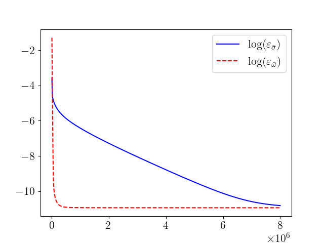
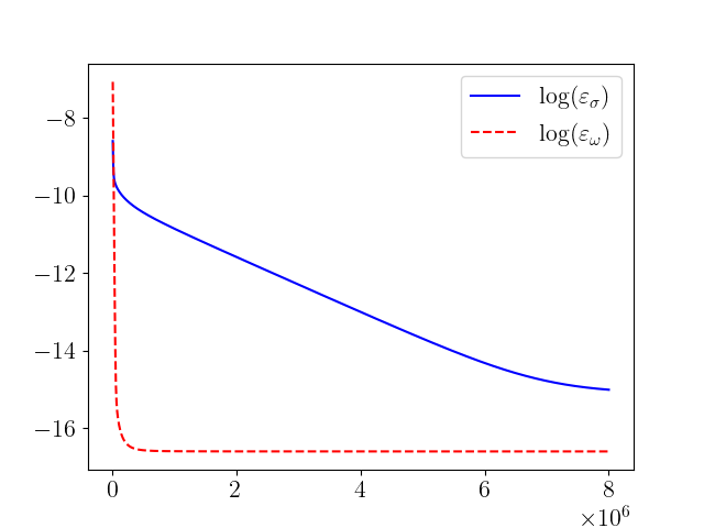
Figure 3: Convergence of the parabolic flow to stationary state as a function of time steps for the solution with $N_{h}=40$ in Table 1.

Also, the regularity of the solution at this final time is checked by computing $\Delta q,$ as defined in (17), by path integrating around the horizon from just above the upper pole to just below the lower pole. As it can be seen, the violation of regularity turns out to be extremely small. The final values of the relative errors for all the runs in this series, together with the values of $\Delta q$ are shown in table 1.

$N_{h}$	$L$	$\varepsilon_{\bar{\sigma}}$	$\varepsilon_{\bar{\omega}}$	$\varepsilon_{\sigma}$	$\varepsilon_{\omega}$	$\Delta q$
22	8.8798	2.19$\times 10^{-6}$	1.40$\times 10^{-6}$	7.94$\times 10^{-8}$	3.22$\times 10^{-9}$	-6.66$\times 10^{-15}$
28	6.9770	2.21$\times 10^{-5}$	4.83$\times 10^{-6}$	1.31$\times 10^{-7}$	1.29$\times 10^{-8}$	-4.17$\times 10^{-14}$
34	5.7457	2.46$\times 10^{-5}$	1.06$\times 10^{-5}$	2.34$\times 10^{-7}$	3.25$\times 10^{-8}$	-5.10$\times 10^{-14}$
40	4.8839	2.01$\times 10^{-5}$	1.78$\times 10^{-5}$	3.04$\times 10^{-7}$	6.19$\times 10^{-8}$	-1.50$\times 10^{-13}$
46	4.2468	1.59$\times 10^{-5}$	2.62$\times 10^{-5}$	3.84$\times 10^{-7}$	1.03$\times 10^{-7}$	2.49$\times 10^{-14}$
50	3.9071	1.47$\times 10^{-5}$	3.27$\times 10^{-5}$	4.89$\times 10^{-7}$	1.40$\times 10^{-7}$	4.39$\times 10^{-14}$
52	3.7568	1.47$\times 10^{-5}$	3.63$\times 10^{-5}$	5.77$\times 10^{-7}$	1.62$\times 10^{-7}$	4.59$\times 10^{-14}$
54	3.6177	1.52$\times 10^{-5}$	4.01$\times 10^{-5}$	7.07$\times 10^{-7}$	1.87$\times 10^{-7}$	-2.07$\times 10^{-13}$
56	3.4885	1.63$\times 10^{-5}$	4.42$\times 10^{-5}$	9.04$\times 10^{-7}$	2.16$\times 10^{-7}$	-8.26$\times 10^{-14}$
58	3.3682	1.83$\times 10^{-5}$	4.87$\times 10^{-5}$	1.22$\times 10^{-6}$	2.48$\times 10^{-7}$	-1.32$\times 10^{-13}$
60	3.2559	2.17$\times 10^{-5}$	5.36$\times 10^{-5}$	1.75$\times 10^{-6}$	2.85$\times 10^{-7}$	-2.35$\times 10^{-13}$

Table 1: Relative error after $8\times 10^{6}$ time steps and violation of regularity, $\Delta q,$ for the solutions in the series.

We choose the run with $L=4.8839$ (corresponding to $N_{h}=40$) as an example to show the plots of the solution and relevant functions, Figure 4 shows the plots of ${\bar{\sigma}}$, ${\bar{\omega}}$, $\sigma$ and $\omega$.

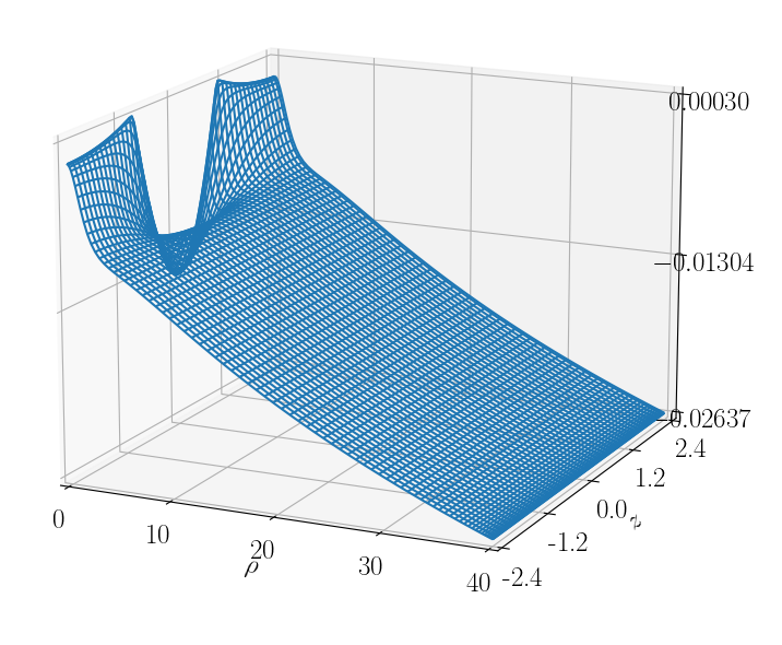
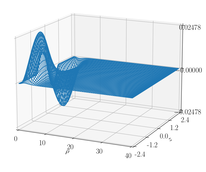
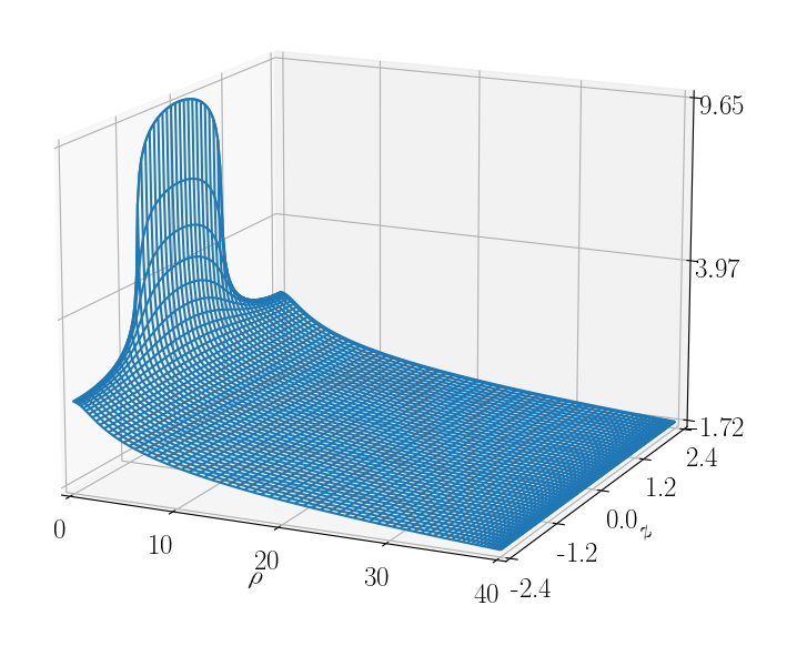
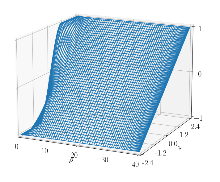
Figure 4: Plots of the solution corresponding to $L=4.8839$ of Table 1. From left to right, from top to bottom: ${\bar{\sigma}}$, ${\bar{\omega}}$, $\sigma$, $\omega$.

Mass, angular velocity and Kasner parameter.

At the final time we compute, for every solution, several relevant quantities. The mass $M$ is computed as the integral $M(\rho_{\rm MAX})$. The horizon’s angular velocity is obtained as the averaged value of $\Omega(\rho=0)$ in one of the horizons.. We also compute the Kasner exponent in two different ways: the first value is obtained from the Mass, as $4M/L$, while the second value is obtained from the asymptotic behaviour of the function $V$; more precisely, as the slope of a linear regression of $\ln(V)$ as function of $\ln(\rho)$ in the asymptotic region of the computational domain, see (12). We arbitrarily define the asymptotic region of the domain as the portion of the domain, adjacent to $\rho_{\rm MAX},$ corresponding to 30% of $\rho$ grid points. The two values obtained for the Kasner exponent are in very good agreement. All these quantities, for the solutions in this series are shown in Table 2.

$L$	$M$ (mass)	Angular velocity	$\alpha$ (from $M$)	$\alpha$ (from $V$)
8.8798	1.0095	6.5753$\times 10^{-2}$	4.5476$\times 10^{-1}$	4.5477$\times 10^{-1}$
6.9770	1.0119	7.0513$\times 10^{-2}$	5.8014$\times 10^{-1}$	5.8017$\times 10^{-1}$
5.7457	1.0164	7.9507$\times 10^{-2}$	7.0758$\times 10^{-1}$	7.0768$\times 10^{-1}$
4.8839	1.0250	9.6689$\times 10^{-2}$	8.3947$\times 10^{-1}$	8.3977$\times 10^{-1}$
4.2468	1.0422	1.3130$\times 10^{-1}$	9.8167$\times 10^{-1}$	9.8264$\times 10^{-1}$
3.9071	1.0640	1.7495$\times 10^{-1}$	1.0893	1.0916
3.7568	1.0807	2.0831$\times 10^{-1}$	1.1506	1.1541
3.6177	1.1036	2.5413$\times 10^{-1}$	1.2202	1.2257
3.4885	1.1358	3.1881$\times 10^{-1}$	1.3024	1.3113
3.3682	1.1831	4.1348$\times 10^{-1}$	1.4050	1.4201
3.2559	1.2557	5.5907$\times 10^{-1}$	1.5426	1.5698

Table 2: Relevant quantities computed for the solutions in the series.

Figure 5 shows the plots of relevant metric functions obtained for the solution corresponding to $N_{h}=40.$

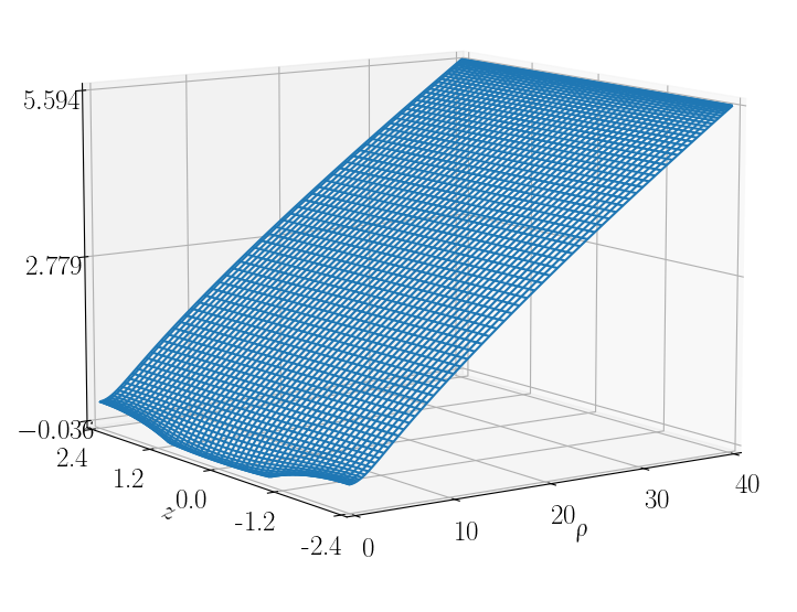
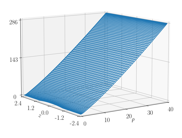
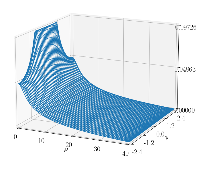
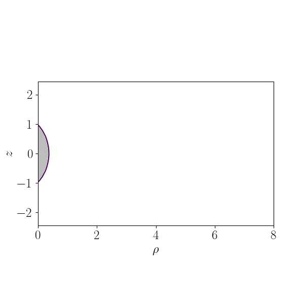
Figure 5: Plots of the metric functions $V$ (top left) and $\eta$ (top right), and plot of $\Omega$ and the ergosphere (as a gray region) at the bottom, for the solution with $N_{h}=40$ of Table 1.

The Smarr identity.

We found that an very sensitive test for checking the computations is the validity of the Smarr identity, this is, the constancy of $M(\rho)$ (see equation 28) as a function of $\rho$. In this sense the plot of $M(\rho)$ became crucial to test to correctness of the outer boundary condition for ${\bar{\sigma}}.$ In Figure 6 we show plots that compare $M(\rho)$ computed for the seed (initial data for the flow) and $M(\rho)$ at final time for the six numerically computed solutions with larger $L$ in the series.

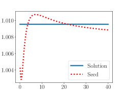
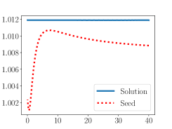
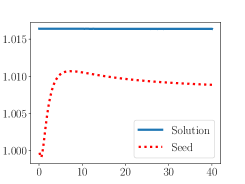
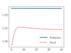
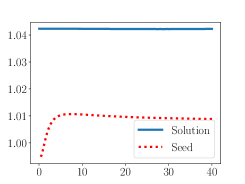
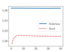
Figure 6: Plots of $M(\rho)$ for the seed and for the numerically computed solution compared for six of the solutions in the series. From left to right from top to bottom the plots correspond to the cases with $Nh=22,28,34,40,46,50$ in Table 1.

Best fitting asymptotic models

We want to check which of the asymptotic candidate solutions fits better the numerically computed solution. To this end, we take the average on the $z$ axis for the function $\eta$ as to get a $z$ independet function $\bar{\eta}(\rho).$ We then compute the best fitting model $\eta$-function for the six posibilities given by models (I$+$), (I$-$), (II$+$), (II$-$), (III$+$) and (III$-$) (see equations (8), (9), and (10)). To do this we minimize the deviation of the model $\eta(a,b,\rho)$ from $\bar{\eta}$ by varying the parameter $a$, or taking $a=0$ for the models (II), and choosing $b$ in such a way that $\eta$ functions are coincident at the outer boundary. We meassure the mentioned deviation by computing the integrated square difference in the asymptotic region:

$$\Delta\eta=\int_{\mbox{asympt. region}}\Bigl{(}\bar{\eta}(\rho)-\eta(a,b,\rho)\Bigr{)}^{2}\leavevmode\nobreak\ d\rho.$$

The results of fitting the eleven solutions in Table 1 are shown in Table 3.

	(III$+$)			(II$+$)		(I$+$)
$L$	$a$	$b$	$\Delta\eta$	$b$	$\Delta\eta$	$a$	$b$	$\Delta\eta$
8.8798	0.5451	2.6149	2.4$\times 10^{-7}$	89.9297	5.2$\times 10^{1}$	0.0001	0.0090	5.2$\times 10^{1}$
6.9770	0.4194	2.2513	1.4$\times 10^{-7}$	49.4932	1.6$\times 10^{1}$	0.0001	0.0049	1.6$\times 10^{1}$
5.7457	0.2906	1.8077	9.0$\times 10^{-9}$	26.8568	3.2	0.0001	0.0027	3.2
4.8839	0.1500	1.1372	1.5$\times 10^{-8}$	13.7707	2.3$\times 10^{-1}$	0.0001	0.0014	2.3$\times 10^{-1}$
4.2468	0.0001	0.0006	6.5$\times 10^{-2}$	6.0951	6.5$\times 10^{-2}$	0.1005	1.0170	6.0$\times 10^{-7}$
3.9071	0.0001	0.0003	2.9$\times 10^{-1}$	2.8198	2.9$\times 10^{-1}$	0.1536	0.9808	4.3$\times 10^{-2}$
3.7568	0.0001	0.0002	4.0$\times 10^{-1}$	1.5649	4.0$\times 10^{-1}$	0.1903	0.8483	8.5$\times 10^{-2}$
3.6177	0.0001	0.0001	5.0$\times 10^{-1}$	0.5104	5.0$\times 10^{-1}$	0.2381	0.6756	1.3$\times 10^{-1}$
3.4885	0.0001	-0.0000	5.9$\times 10^{-1}$	-0.3766	5.9$\times 10^{-1}$	0.3019	0.4511	1.6$\times 10^{-1}$
3.3682	0.0001	-0.0001	6.5$\times 10^{-1}$	-1.1241	6.5$\times 10^{-1}$	0.3898	0.1107	1.9$\times 10^{-1}$
3.2559	0.0001	-0.0002	7.1$\times 10^{-1}$	-1.7558	7.1$\times 10^{-1}$	0.5172	-0.3566	2.1$\times 10^{-1}$
	(I$-$)			(II$-$)		(III$-$)
$L$	$a$	$b$	$\Delta\eta$	$b$	$\Delta\eta$	$a$	$b$	$\Delta\eta$
8.8798	0.0106	1.4862	5.4$\times 10^{1}$	97.3074	5.6$\times 10^{1}$	0.0001	0.0097	5.6$\times 10^{1}$
6.9770	0.0188	1.6213	1.7$\times 10^{1}$	56.8710	1.9$\times 10^{1}$	0.0001	0.0057	1.9$\times 10^{1}$
5.7457	0.0327	1.6434	4.2	34.2346	5.1	0.0001	0.0034	5.1
4.8839	0.0572	1.7306	5.9$\times 10^{-1}$	21.1485	1.1	0.0001	0.0021	1.1
4.2468	0.1022	1.9351	3.6$\times 10^{-3}$	13.4728	1.4$\times 10^{-1}$	0.0001	0.0013	1.4$\times 10^{-1}$
3.9071	0.1250	1.4114	8.5$\times 10^{-9}$	10.1975	2.1$\times 10^{-2}$	0.0001	0.0010	2.1$\times 10^{-2}$
3.7568	0.1164	1.0874	1.6$\times 10^{-9}$	8.9426	5.8$\times 10^{-3}$	0.0001	0.0009	5.8$\times 10^{-3}$
3.6177	0.0909	0.7270	1.1$\times 10^{-9}$	7.8882	8.4$\times 10^{-4}$	0.0001	0.0008	8.4$\times 10^{-4}$
3.4885	0.0001	0.0007	2.3$\times 10^{-7}$	7.0012	2.3$\times 10^{-7}$	0.0147	0.1029	1.4$\times 10^{-9}$
3.3682	0.0001	0.0006	2.6$\times 10^{-4}$	6.2537	2.6$\times 10^{-4}$	0.1089	0.6775	2.2$\times 10^{-9}$
3.2559	0.0001	0.0006	4.7$\times 10^{-4}$	5.6220	4.7$\times 10^{-4}$	0.1629	0.9108	3.3$\times 10^{-9}$

Table 3: Fit of the solutions of Table 1 with the six possible models given by equations (8),(9), and (10).

It is very interesting to see how well the $z$-averaged $\eta$ function of our numerically computed solution fits, in the whole $\rho$ range, one of the model $\eta$ functions. As expected, for large values of $L$ the best fiting model is (III$+$). Then, for decreasing values of $L$ the best fitting model becomes (I$+$), then to (I$-$) and finally (III$-$). Figure 7 show six examples taken from Table 3.

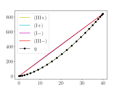
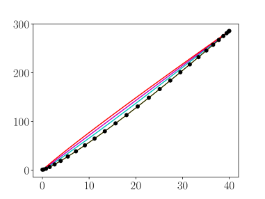
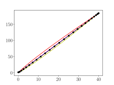
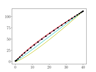
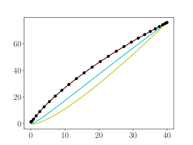
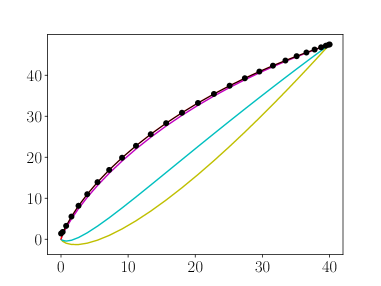
Figure 7: Plots of $\bar{\eta}$ together with the fitting models (III$+$), (I$+$), (I$+$) and (III$+$) for the six solutions in Table 3 corresponding, from left to right, from top to bottom, to $L=8.8798,\leavevmode\nobreak\ 4.8839,\leavevmode\nobreak\ 4.2468,\leavevmode\nobreak\ 3.7568,\leavevmode\nobreak\ 3.4885,\leavevmode\nobreak\ 3.2559$. The $\bar{\eta}$ curve overlaps the best fitting model in all cases, while some of the bad fitting model curves also overlap, that is why no all curves are visible in all plots.

The Smarr formula, presented in the usual form, is

$$M=\frac{1}{4\pi}\kappa A+2\Omega_{\mathcal{H}}J,$$ (44)

where $M$ and $J$ are the Komar mass and angular momentum, respectively, $\kappa$ is the horizon temperature, $A$ is the horizon area and $\Omega_{\mathcal{H}}$ is the horizon angular velocity. Since the solutions that reach infinity are those in family (III+), we have that Smarr formula reduces to

$$(1-a)L/4=\frac{1}{4\pi}\kappa A+2\Omega_{\mathcal{H}}J,$$ (45)

where $0<a\leq 1$. This positivity of $a$ allows us to obtain an interesting bound for $L$, since it can be shown $\Omega_{\mathcal{H}}J>0$, forcing

$$0<2\Omega_{\mathcal{H}}J\leq\frac{L}{4}-\frac{1}{4\pi}\kappa A=\frac{L}{4}-m.$$ (46)

Therefore, there are no solution that extend to infinity whenever $L<4m$. As we are checking with the numerical analysis, this is a rough lower bound for the critical $L$.

Ergosphere merging.

For large values of $L,$ ergospheric region associated to the horizon does not touch the $z=\pm L/2$ boundaries of the domain. This ergosphere is topologically $S^{2}$. When the value of $L$ decreases the ergospheric region get closer to the boundaries and at some point touches them. In other words the ergosphere becomes topologically a torus $T^{2}$. This change in the topology of the ergosphere is not new, as it has been studied in binary systems, so is not a surprise to see a development of such behaviour in the periodic set up. This process is shown in Figure 8.

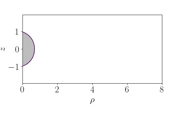
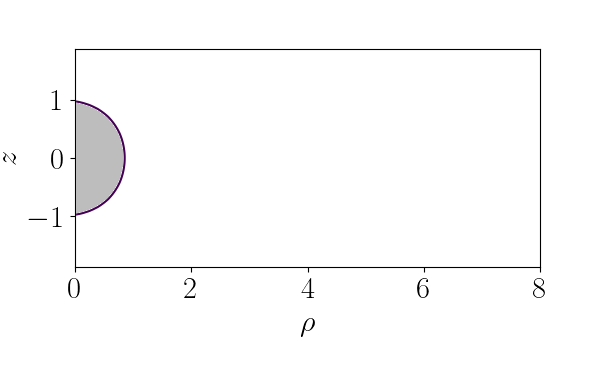
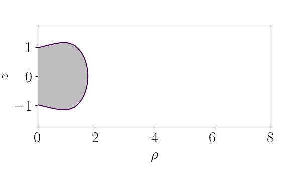
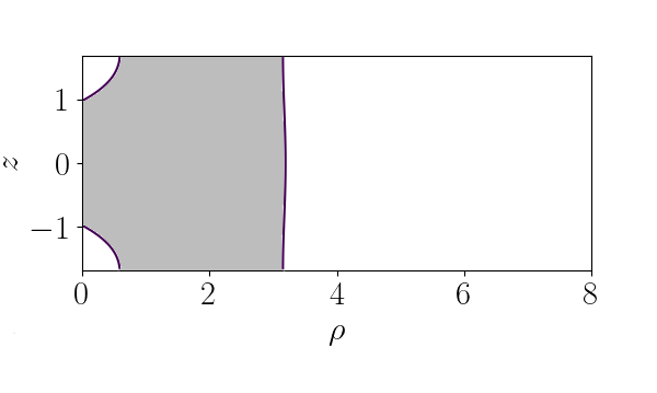
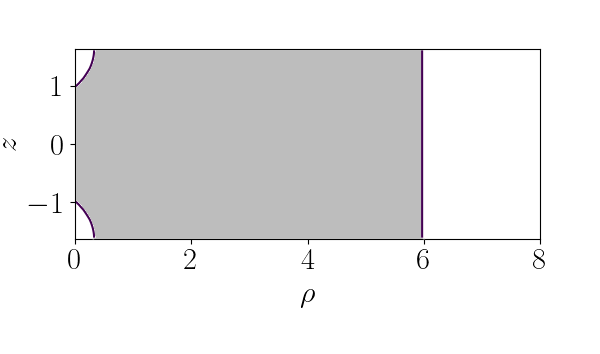
Figure 8: The shaded regions are the ergospheres of the last six solutions of Table 1. From left to right, from top to bottom the six plots correspond $L=8.8798,\leavevmode\nobreak\ 4.8839,\leavevmode\nobreak\ 4.2468,\leavevmode\nobreak\ 3.7568,\leavevmode\nobreak\ 3.4885,\leavevmode\nobreak\ 3.2559$.

4.2 Second series: $J=1/2$

We include here, for the sake of comparison, results corresponding to a series of four solutions with a higher value of $J$ and the same horizon’s area as the previous series. The three solutions with larger value of $L$ are better fitted by the asymptotic model (III$+$) of (10), while the solution with $L=4.5475$ is is better fitted with the model (I$+$) of equation (8).

In table 4 the relevant physical quantities of the solutions in this series are shown.

$N_{h}$	$L$	$M$ (mass)	Angular velocity	$\alpha$ (from $M$)	$\alpha$ (from $V$)
22	8.2683	1.0391	1.3024$\times 10^{-1}$	5.0272$\times 10^{-1}$	5.0278$\times 10^{-1}$
28	6.4965	1.0518	1.4287$\times 10^{-1}$	6.4761$\times 10^{-1}$	6.4781$\times 10^{-1}$
32	5.3501	1.0775	1.6860$\times 10^{-1}$	8.0560$\times 10^{-1}$	8.0632$\times 10^{-1}$
40	4.5475	1.1340	2.2516$\times 10^{-1}$	9.9745$\times 10^{-1}$	1.0003

Table 4: Relevant quantities computed for solutions with $J=1/2$.

5 Conclusions

In this work we present numerical solutions of the Einstein equations in a periodic set up, for stationary, coaxial and periodic co-rotating black holes, improving the knowledge of stationary solutions outside the standard asymptotically flat scenario and trivial topology. The solutions add angular momentum to the important Myers/Korotkin-Nicolai configurations of static, coaxial and periodic black holes, thus realizing a periodic analogue of the Kerr solution. The solution space contains a rich structure, sharing many qualitative and quantitative properties with the family of Stockum infinite rotating cylinders.

Periodic Kerr solutions and Stockum solutions have both Lewis asymptotic. Furthermore, both families posses a critical phenomenon: in the case of periodic Kerr we find that numerical solutions with a given value for the area $A$ and for the angular momentum $J$ of the horizons appear to exist only when the separation between consecutive horizons is larger than a certain critical value that depends only on $A$ and $|J|$. Below the mentioned critical value the rotational energy appears to be too big to sustain a global equilibrium and a singularity shows up at a finite distance from the bulk. For Stockum cylinders, instead, the asymptotic collapse manifest when the angular momentum (per unit of length) reaches a critical value compared to the mass (per unit of length). In both families the collapse is through a transition in the Lewis models of asymptotic.

The Smarr identity proved to be a powerful tool to define an appropriate Neumann-like asymptotic boundary condition for the harmonic map heat flow. This new dynamical Neumann condition can be used in other periodic configurations, for example in periodic arrangements of counter-rotating black holes, situation that we are presently investigating. In this case, the asymptotic model is not that of a rotating rod, but Kasner as the MKN family. The solution space seems to have quite different properties. This in particular poses interesting questions regarding the collapse of the asymptotic and the existence of solutions when the horizons get closer.

This work explores several features which are important in black hole physics in other contexts as well, such as string theory [18, 19, 20, 21, 22, 23], supergravity [24, 25] and binary solutions [26, 27, 28, 29].

Appendix A Simple deduction of Lewis’s models

Assume then that $\partial_{z}$ is a Killing field so that the metric coefficient $V,W,\eta$ and $\gamma$ are $z$-independent. This implies that $\sigma$ is independent of $z$ and it is simple to see that $\omega$ must be independent of $\rho$. The equations for $\sigma$ and $\omega$ thus become,

$$\partial^{2}_{\rho}\sigma+\frac{1}{\rho}\partial_{\rho}\sigma=-\frac{e^{-2\sigma}(\partial_{z}\omega)^{2}}{\rho^{4}},\quad\partial^{2}_{z}\omega=0.$$ (47)

Hence $\omega=wz+w_{1}$ with $w\neq 0$ and $w_{1}$ constants. Therefore,

$$\partial^{2}_{\rho}\sigma+\frac{1}{\rho}\partial_{\rho}\sigma=-\frac{e^{-2\sigma}w^{2}}{\rho^{4}}.$$ (48)

After making the change of variables $\bar{u}=-\sigma-\ln\rho$ the previous equation implies,

$$\left(\rho\bar{u}^{\prime}\right)^{2}=w^{2}e^{2\bar{u}}+C,$$ (49)

where ${}^{\prime}=d/d\rho$. The sign of the constant $C$ will be relevant. Set $C=\epsilon a^{2}$, with $a\geq 0$ and $\epsilon=-1,1$.

Now, letting $x=e^{-\bar{u}}(=\eta/\rho)$ and defining the new variable $\zeta=\ln\rho/\rho_{0}$ (for some $\rho_{0}>0$), we arrive at (we use $\partial_{\zeta}x=\dot{x}$), $\dot{x}^{2}=w^{2}+\epsilon a^{2}x^{2}$, to obtain after $\zeta$-derivation,

$$\ddot{x}=\epsilon a^{2}x.$$ (50)

Figure 9: Types of $x-$orbits in phase space $(x,\dot{x})$.

There are three types of solutions:

1. For $a=0$, we have,

   $$x=|w|\left(\pm\ln\rho+b\right),$$ (51)

2. For $a>0$ and $\epsilon=-1$, we have,

   $$x=\frac{|w|}{a}\sin(\pm a\ln\rho+b),$$ (52)

3. For $a>0$ and $\epsilon=1$, we have,

   $$x=\frac{|w|}{a}\sinh(\pm a\ln\rho+b).$$ (53)

   In the three cases $b$ is an arbitrary constant.

References

- [1] Roberto Emparan and Harvey S. Reall. A Rotating black ring solution in five-dimensions. Phys. Rev. Lett., 88:101101, 2002.
- [2] Henriette Elvang and Pau Figueras. Black Saturn. JHEP, 05:050, 2007.
- [3] Marcus Khuri, Gilbert Weinstein, and Sumio Yamada. 5-Dimensional Space-Periodic Solutions of the Static Vacuum Einstein Equations. JHEP, 12:002, 2020.
- [4] Marcus Khuri, Gilbert Weinstein, and Sumio Yamada. Balancing Static Vacuum Black Holes with Signed Masses in 4 and 5 Dimensions. Phys. Rev. D, 104:044063, 2021.
- [5] R. C. Myers. Higher-dimensional black holes in compactified space-times. Phys. Rev. D, 35:455–466, Jan 1987.
- [6] D. Korotkin and H. Nicolai. A Periodic analog of the Schwarzschild solution. 3 1994.
- [7] D. Korotkin and H. Nicolai. The Ernst equation on a Riemann surface. Nucl. Phys. B, 429:229–254, 1994.
- [8] Roberto Emparan and Harvey S. Reall. Black Holes in Higher Dimensions. Living Rev. Rel., 11:6, 2008.
- [9] B. Mavrin. The Search for the Compactified Kerr Solution. Concordia University, 2015.
- [10] Thomas Lewis. Some special solutions of the equations of axially symmetric gravitational fields. Proc. R. Soc. Lond., 57:135–154, 1932.
- [11] Willem Jacob van Stockum. The gravitational feild of a distribution of particles rotating about an axis of symmetry. Proc. Roy. Soc. Edinburgh A, 136:176–192, 1937.
- [12] Gilbert Weinstein. On rotating black holes in equilibrium in general relativity. Communications on Pure and Applied Mathematics, 43(7):903–948, 1990.
- [13] Sergio Dain and Omar E. Ortiz. Numerical evidences for the angular momentum-mass inequality for multiple axially symmetric black holes. Phys. Rev. D, 80:024045, Jul 2009.
- [14] Andrei V. Frolov and Valeri P. Frolov. Black holes in a compactified space-time. Phys. Rev. D, 67:124025, 2003.
- [15] S. Labrosse and A. Morison. dmsuite: A collection of spectral collocation differentiation matrices. https://github.com/labrosse/dmsuite, 2018.
- [16] L. N. Trefethen. Spectral Methods in MATLAB. SIAM, 2000.
- [17] Elsayed M.E. Elbarbary and Salah M. El-Sayed. Higher order pseudospectral differentiation matrices. Applied Numerical Mathematics, 55(4):425–438, 2005.
- [18] Ashoke Sen. Black hole solutions in heterotic string theory on a torus. Nucl. Phys. B, 440:421–440, 1995.
- [19] Ramzi R. Khuri. Black holes and solitons in string theory. Helv. Phys. Acta, 67:884–922, 1994.
- [20] Valeri P. Frolov. Black holes and cosmic strings. In 6th APCTP Winter School on Black Hole Astrophysics 2002, pages 39–58, 1 2002.
- [21] G. W. Gibbons and D. L. Wiltshire. Black Holes in Kaluza-Klein Theory. Annals Phys., 167:201–223, 1986. [Erratum: Annals Phys. 176, 393 (1987)].
- [22] Finn Larsen. Kaluza-Klein black holes in string theory. In 7th International Symposium on Particles, Strings and Cosmology, pages 57–66, 12 1999.
- [23] Finn Larsen. Rotating Kaluza-Klein black holes. Nucl. Phys. B, 575:211–230, 2000.
- [24] Robert C. Myers. Superstring Gravity and Black Holes. Nucl. Phys. B, 289:701–716, 1987.
- [25] Jaemo Park. Black hole solutions of Kaluza-Klein supergravity theories and string theory. Class. Quant. Grav., 15:775–785, 1998.
- [26] Vladimir Manko, E. Rodchenko, E. Ruiz, and Boris Sadovnikov. Exact solutions for a system of two counter-rotating black holes. Phys. Rev. D, 78, 12 2008.
- [27] Vladimir Manko, E. Ruiz, and M. Sadovnikova. Stationary configurations of two extreme black holes obtainable from the kinnersley-chitre solution. Physical Review D - PHYS REV D, 84, 05 2011.
- [28] Vladimir Manko and E. Ruiz. Metric for two equal kerr black holes. Physical Review D, 96, 02 2017.
- [29] Marco Astorino and Adriano Viganò. Charged and rotating multi-black holes in an external gravitational field. Eur. Phys. J. C, 82(9):829, 2022.