Coalescence and sampling distributions for Feller diffusions

Abstract

Consider the diffusion process defined by the forward equation $u_{t}(t,x)=\tfrac{1}{2}\{xu(t,x)\}_{xx}-\alpha\{xu(t,x)\}_{x}$ for $t,x\geq 0$ and $-\infty<\alpha<\infty$, with an initial condition $u(0,x)=\delta(x-x_{0})$. This equation was introduced and solved by Feller to model the growth of a population of independently reproducing individuals. We explore important coalescent processes related to Feller’s solution. For any $\alpha$ and $x_{0}>0$ we calculate the distribution of the random variable $A_{n}(s;t)$, defined as the finite number of ancestors at a time $s$ in the past of a sample of size $n$ taken from the infinite population of a Feller diffusion at a time $t$ since since its initiation. In a subcritical diffusion we find the distribution of population and sample coalescent trees from time $t$ back, conditional on non-extinction as $t\to\infty$. In a supercritical diffusion we construct a coalescent tree which has a single founder and derive the distribution of coalescent times.

1 Introduction

Feller [12, 13, Section 5] introduced the process governed by the diffusion equation

$$u_{t}(t,x)=\tfrac{1}{2}\{xu(t,x)\}_{xx}-\alpha\{xu(t,x)\}_{x},\qquad 0\leq x<\infty,\;\alpha\in\mathbb{R},$$ (1)

as the continuum analogue of a classical branching process, primarily with the intention of modelling the growth of a population of statistically independently reproducing individuals. This stochastic process has subsequently found broader applications in biology, genetics, ecology, nuclear physics, statistical physics, seismology and finance (see Gan and Waxman [16, Section I] for a detailed list of references).

In the present paper we are interested in the Feller diffusion as the continuum limit of a Bienaymé-Galton-Watson (BGW) process, and applications to population genetics including sampling distributions of populations undergoing neutral mutations between multiple types. Our approach is based on the coalescent. In common with the diffusion limit of the Wright-Fisher and Moran coalescent trees, the coalescent of a Feller diffusion has the property that it ‘comes down from infinity’. That is to say, the entire, uncountably infinite, population at any time chosen as the present has a finite number of ancestral lineages at any positive time in the past (see Fig. 1). The key step in our analysis is Theorem 1 in which we calculate the distribution of the discrete random variable $A_{\infty}(s;t)$, defined to be the number of ancestors at an earlier time $t-s$ of the entire population at the current time $t$ since initiation of the process.

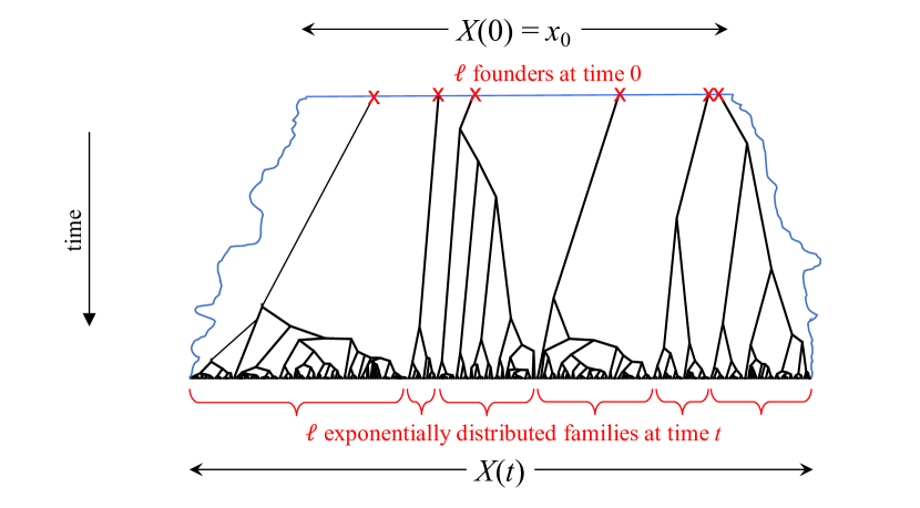
Figure 1: Structure of the ancestral tree of a Feller diffusion conditioned on $X(0)=x_{0}$. The ancestry of the population $X(t)$ “comes down from infinity”, that is, the number of ancestors (black lines) of the currently observed infinite population at any finite time in the past is finite. The blue lines either side represent the entire, infinite population at earlier times, most of whose descendant lines become extinct by time $t$. The final population is the sum of a Poisson number of independent exponentially distributed family sizes (see Eq. (2.3)).

Starting from this theorem we follow two paths. In the first we consider the limit $t\to\infty$ at fixed $s$ of a subcritical Feller diffusion conditioned on survival of the population. Results for expected inter-coalescent waiting times for a random sample agree with a recent, less straightforward derivation using the Laplace transform by Burden and Griffiths [6].

The second path involves taking the limit $s\to 0$ at fixed $t$. At any $s>0$ we find that the ancestry of the process over the interval $[0,t-s]$ is equivalent to the ancestry of a homogeneous birth-death (BD) process with $s$-dependent birth and death rates. Both of these rates become infinite as $s\to 0$ while their difference remains constant and equal to the parameter $\alpha$. Useful tools for characterising the properties of coalescent trees generated by a homogeneous birth-death (BD) process are the reconstructed process (RP) [25] and the reversed-reconstructed process (RRP) [2, 17, 27, 28, 19], which assumes an improper prior on the time since initiation of the process, starting with a single ancestor. We construct the coalescent tree for a Feller diffusion as the limit of a RP from a linear BD process, and from this construct a RRP for the supercritical process and hence calculate the distribution of coalescent times.

Previously Burden and Simon [7] and Burden and Soewongsono [8] have studied coalescence of the supercritical Feller diffusion from a frequentist point of view, in the sense that they calculate confidence intervals on the time since initiation and initial parameters of the Feller diffusion in terms of a later observation. The current paper is complementary in that the analysis of the supercritical diffusion is Bayesian in that the RRP requires a uniform prior on the time since initiation of the ancestral tree.

The Feller diffusion is implicit within the near-critical continuum limit of a continuous-time BGW process studied by O’Connell [26] and [18], who also calculate distributions of coalescent times. However their analysis differs in that it assumes a process initiated by a single progenitor, their near-critical limit consists of taking the time since initiation to infinity while keeping the branching time and reproduction rate constant, and results are stated in terms of the fraction of time since initiation. These differences make direct comparison with the current work problematic, though within the text of this paper we will note connections with O’Connell [26] where appropriate.

Crespo et al. [10] analyse coalescence in the infinite population limit of a RRP constructed from a BD process. Their limiting process differs from the $s\to 0$ diffusion limit in the current paper in that the time axis is rescaled. Numerical simulations of their coalescent model employ further approximations which amount to setting the population size as a deterministic function rather a stochastic process.

The layout of the paper is as follows. In Section 2 we summarise properties of the Feller diffusion including its connection with continuum limits of BD and BGW processes and the interpretation of Feller’s solution. This establishes known results and a notation required for subsequent sections. In Section 3 distributions are derived for $A_{n}(s,\;t)$, defined to be the number of ancestors at an earlier time $t-s$ of the entire population at the current time $t$ since initiation of the process, and for the corresponding count $A_{\infty}(s;t)$ of the number of ancestors of the entire population at time $t$. The limit $t\to\infty$ at fixed $s$ of a sub-critical Feller diffusion conditioned on survival and the quasi-stationary sampling distribution are dealt with in Section 4. The limit $s\to 0$ at fixed $t$ and the connection between the RP of a BD process and the coalescent tree of a Feller diffusion are dealt with in Section 5. In Section 6 the coalescent tree for the entire population generated by a a supercritical Feller diffusion is constructed as a RRP, from which the distributions of coalescent times for the population and for a finite sample are calculated in Section 7. Results are summarised in Section 8.

2 Properties of the Feller Diffusion

For any bounded continuous function $g$ with second derivatives existing, a standard backward Kolmogorov equation for a stochastic process $X(t)$ is

$$\frac{d}{dt}\mathbb{E}\left[g(X(t))\right]=\mathbb{E}\left[{\cal L}g(X(t))\right],$$

where the right side is the expectation of the function $h$ defined by $h={\cal L}g$. The operator $\cal L$ is referred to as the generator of the process. In general, if a continuous random variable $X(t)$ evolves so that

$$\begin{split}\mathbb{E}\left[X(t+\delta t)-X(t)\mid X(t)=x\right]&=a(x)\delta t+o(\delta t),\\ \mathbb{E}\left[(X(t+\delta t)-X(t))^{2}\mid X(t)=x\right]&=b(x)\delta t+o(\delta t),\\ \mathbb{E}\left[(X(t+\delta t)-X(t))^{k}\mid X(t)=x\right]&=o(\delta t),\quad k\geq 3,\\ \end{split}$$ (2)

as $\delta t\to 0$, then the generator takes the form 22, p214; 11, Chapter 4

$${\cal L}=\tfrac{1}{2}b(x)\frac{\partial^{2}}{\partial x^{2}}+a(x)\frac{\partial}{\partial x}.$$

For the particular case $a(x)=\alpha x$, $b(x)=x$ we refer to the process with generator

$${\cal L}=\tfrac{1}{2}x\frac{\partial^{2}}{\partial x^{2}}+\alpha x\frac{\partial}{\partial x},$$ (3)

as a Feller diffusion [13, 14]. The process is said to be sub-critical, critical or super-critical if $\alpha<0$, $\alpha=0$ or $\alpha>0$ respectively. A Feller diffusion can arise as a limit of a BD process or as a limit of a BGW process.

2.1 Feller Diffusion as the limit of a BD process

Baake and Wakolbinger [4] argue that Feller [13] regarded Eq. (1) primarily in terms of the large-population, near-critical limit of a continuous-time BD process. In Proposition 1 we set out details of how this limit scales, using notation which will prove useful in Section 5.

Consider a linear BD process with birth rate $\hat{\lambda}(\epsilon)$ and death rate $\hat{\mu}(\epsilon)$ specified as functions of a parameter $\epsilon\in\mathbb{R}_{\geq 0}$ with the property

$$\begin{split}\hat{\lambda}(\epsilon)&=\tfrac{1}{2}\epsilon^{-1}+\tfrac{1}{2}\alpha+\mathcal{O}(\epsilon),\\ \hat{\mu}(\epsilon)&=\tfrac{1}{2}\epsilon^{-1}-\tfrac{1}{2}\alpha+\mathcal{O}(\epsilon),\end{split}$$

as $\epsilon\to 0$. If $M_{\epsilon}(t)$ is the number of particles alive at time $t$, then for $n,y=0,1,2,\ldots$,

$$p_{n,y} := \mathbb{P}\left(M_{\epsilon}(t+\delta t)=y\mid M_{\epsilon}(t)=n\right)$$ (4)

$$= \begin{cases}n\hat{\lambda}\delta t+\mathcal{O}(\delta t^{2}),&y=n+1;\\ 1-n(\hat{\lambda}+\hat{\mu})\delta t+\mathcal{O}(\delta t^{2}),&y=n;\\ n\hat{\mu}\delta t+\mathcal{O}(\delta t^{2}),&y=n-1;\\ \mathcal{O}(\delta t^{2}),&\mbox{otherwise.}\end{cases}$$

Proposition 1.

Set $X(t)=\epsilon M_{\epsilon}(t)$. Then the limiting generator of the process $X(t)$ as $\epsilon\to 0$ is the Feller diffusion generator Eq. (3).

Proof.

With $x=\epsilon n$ consider the simultaneous limit $\epsilon\to 0$, $n\to\infty$ at fixed $x$:

$$\lim_{\epsilon\to 0,n\to\infty}\mathbb{E}\left[X(t+\delta t)-X(t)\mid X(t)=x\right]$$

$$= \lim_{\epsilon\to 0,n\to\infty}\epsilon(p_{n,n+1}\times 1+p_{n,n}\times 0+p_{n,n-1}\times(-1))$$

$$= \lim_{\epsilon\to 0,n\to\infty}\epsilon\{n(\alpha+\mathcal{O}(\epsilon))\delta t+\mathcal{O}(\delta t^{2})\}$$

$$= \alpha x\delta t+\mathcal{O}(\delta t^{2});$$

$$\lim_{\epsilon\to 0,n\to\infty}\mathbb{E}\left[(X(t+\delta t)-X(t))^{2}\mid X(t)=x\right]$$

$$= \lim_{\epsilon\to 0,n\to\infty}\epsilon^{2}(p_{n,n+1}\times 1+p_{n,n}\times 0+p_{n,n-1}\times 1)$$

$$= \lim_{\epsilon\to 0,n\to\infty}\epsilon^{2}\{n(\epsilon^{-1}+\mathcal{O}(\epsilon))\delta t+\mathcal{O}(\delta t^{2})\}$$

$$= x\delta t+\mathcal{O}(\delta t^{2});$$

and for $k\geq 3$

$$\lim_{\epsilon\to 0,n\to\infty}\mathbb{E}\left[(X(t+\delta t)-X(t))^{k}\mid X(t)=x\right]$$

$$= \lim_{\epsilon\to 0,n\to\infty}\epsilon^{k}(p_{n,n+1}\times 1+p_{n,n}\times 0+p_{n,n-1}\times(-1)^{k})$$

$$= \lim_{\epsilon\to 0,n\to\infty}\epsilon^{k}\{n\mathcal{O}(\epsilon^{-1}\delta t+\mathcal{O}(\delta t^{2})\}$$

$$= o(\delta t),$$

as $\delta t\to 0$, as required. ∎

2.2 Feller Diffusion as the limit of a BGW process

Consider a BGW branching process with discrete generations $i=0,1,2,\ldots$ and population size $Y(i)$ at generation $i$. Assume the numbers of offspring per individual per generation are identically and independently distributed (i.i.d.) random variables $S_{ik}$, $k=1,\ldots,Y(i)$, represented here by a generic random variable $S$ with $\Pr(S=0)>0$, $\mathbb{E}[S]=\lambda,\mbox{$\rm{Var}$\,}(S)=\sigma^{2}$, and finite moments to all orders. Then $Y(i+1)=\sum_{k=1}^{Y(i)}S_{ik}$. We also assume that the process begins with a specified population size $Y(0)=y_{0}$.

More specifically, consider the evolution of the subpopulation $\{M(i)\}_{i\geq 0},$ descended from a subset of of size $m_{0}\leq y_{0}$ of the initial population. A diffusion limit is obtained for a process beginning at $M(0)=m_{0}$, $Y(0)=y_{0}$ by defining a time $t\in\mathbb{R}_{\geq 0}$ and scaled population $X(t)$ such that

$$t=\frac{\sigma^{2}i}{y_{0}}\mbox{ for }i\in\mathbb{Z}_{\geq 0},\quad X(t)=\frac{M(i)}{y_{0}},$$ (5)

and by taking the limit $m_{0},y_{0}\rightarrow\infty$, $\lambda\rightarrow 1$, and $\sigma^{2}$ fixed, in such a way that

$$\alpha:=\frac{y_{0}\log\lambda}{\sigma^{2}}\quad\text{ and }\quad x_{0}:=\frac{m_{0}}{y_{0}}$$ (6)

remain fixed. Equivalently, we require that the mean number of offspring per parent is $\lambda=1+\alpha\sigma^{2}/y_{0}+o(1/y_{0})$ as $y_{0}\to\infty$.

Proposition 2.

The limiting generator of the BGW process $X(t)$ with initial condition $X(0)=x_{0}$, as described above, is the Feller diffusion generator Eq. (3).

That the Feller diffusion can be obtained as the limit of a BGW process is a classical result [9, Example 5.9, p235]. A proof consists of confirming that the functions $a$ and $b$ in Eq. (2), with $\delta t=\sigma^{2}/y_{0}$ corresponding to an increment of one generation, have the required limits. For a details in the context of the forward Kolmogorov equation with slightly different notational conventions see Burden and Simon [7, Section 2].

2.3 Solution to the Feller Diffusion with initial condition $X(0)=x_{0}$

Feller [14, Lemma 9] gives the solution for the density of $X(t)$ for a given initial condition. The method of solution involves solving for the Laplace transform by integrating along characteristics, and is set out in detail in Cox and Miller [9, Section 5.11]. The density of $X(t)$ corresponding to the initial condition $X(0)=x_{0}$ is

$$f_{X(t)}(x;\alpha,x_{0}) = \mathcal{P}(0;x_{0}\mu(t;\alpha))\delta(x)$$

$$+\,\sum_{l=1}^{\infty}\mathcal{P}(l;x_{0}\mu(t;\alpha))\frac{x^{l-1}}{\beta(t;\alpha)^{l}(l-1)!}e^{-x/\beta(t;\alpha)},\quad x\geq 0,$$

where $\delta(x)$ is the Dirac delta function,

$$\mathcal{P}(l;\mu)=e^{-\mu}\frac{\mu^{l}}{l!},\qquad l=0,1,2,\ldots,$$

and

$$\mu(t;\alpha)=\frac{2\alpha e^{\alpha t}}{e^{\alpha t}-1},\qquad\beta(t;\alpha)=\frac{e^{\alpha t}-1}{2\alpha}.$$ (8)

We set $\mu(t;0)=2/t$ and $\beta(t;0)=t/2$. The expansion represents a Poisson-Gamma mixture, with an atom at zero of mass $\exp(-x_{0}\mu(t;\alpha))$, the probability the population of extinction by time $t$, plus a continuous part for $x>0$.

The asymptotic limit as $t\to\infty$ of the atom at zero can be confirmed directly from a classical result stated in Athreya and Ney [3, Theorem 1] for the eventual extinction probability of a BGW process with a single founder. In the notation of Section 2.2, for the process $\{M(i)\}_{i\geq 0}$ with $M(0)=m_{0}$, the eventual extinction probability is

$$\mathbb{P}(M(\infty)=0\mid M(0)=m_{0})=\zeta^{m_{0}},$$ (9)

where $\zeta$ is the smallest non-negative root of the iterative equation $\zeta=G_{S}(\zeta)=\mathbb{E}[e^{\zeta S}]$. Moreover, this extinction probability is $<1$ or $=1$ according as $\lambda=\mathbb{E}[S]$ is $>1$ (supercritical case) or $\leq 1$ (critical or sub-critical cases). To obtain the near-critical limit of Proposition 2, note that the moment generating function satisfies

$$G_{S}(1)=1,\quad G^{\prime}_{S}(1)=\lambda,\quad\text{and }G^{\prime\prime}_{S}(1)=\sigma^{2}+\lambda^{2}-\lambda>0,$$

and hence

$$\zeta=1+\lambda(\zeta-1)+\tfrac{1}{2}(\sigma^{2}+\lambda^{2}-\lambda)(\zeta-1)^{2}+O\left((\zeta-1)^{3}\right),$$

as $\zeta\to 1$. Solving for the smallest non-negative root, and noting that $\zeta$ is close to 1 for $\lambda$ close to 1, we have either $\zeta=1$ if $\lambda\leq 1$, or

$$\zeta = 1+\frac{2(1-\lambda)}{\sigma^{2}}+O\left((\lambda-1)^{2}\right)$$

$$= 1-\frac{2\log\lambda}{\sigma^{2}}+O\left((\log\lambda)^{2}\right)$$

$$= 1-\frac{2\alpha}{y_{0}}+O\left(\frac{1}{y_{0}^{2}}\right),$$

if $\lambda>1$, using Eq. (6) in the last line. From Proposition 2 and Eq. (9), the probability of eventual extinction for a supercritical Feller diffusion is

$$\lim_{y_{0}\rightarrow\infty}\left(1-\frac{2\alpha}{y_{0}}\right)^{x_{0}y_{0}}=e^{-2\alpha x_{0}},$$

agreeing with asymptotic limit of the point mass in Eq. (2.3) for the $\alpha>0$ case. The $\alpha\leq 0$ case corresponds to the $\lambda\leq 1$ stable solution.

The interpretation of the continuous part of Eq. (2.3) is that the population at time $t$ is composed of independent families descended from $L=l$ founders at time $0$, where $L$ is Poisson with mean $x_{0}\mu(t;\alpha)$. The size of each family is an independent exponential random variable with means $\beta(t;\alpha)$, as observed by O’Connell [26, Theorem 2.1(ii)]. See also Harris et al. [18]. Fig. 1 represents a typical ancestry for a non-extinct population $X(t)$ with $l=6$ ancestors.

To understand the origin of this interpretation, consider the limiting process of a BGW process described in Subsection 2.2. The density of the distribution of the descendants of a single individual in the original population is approximated to $\mathcal{O}(1/y_{0})$ by setting $m_{0}$ to 1 in Eq. (6) and hence $x_{0}=1/y_{0}$ in Eq. (2.3):

$$f_{\text{1-family}}(x,t)=\left(1-\frac{\mu(t;\alpha)}{y_{0}}\right)\delta(x)+\frac{\mu(t;\alpha)}{y_{0}}\frac{1}{\beta(t;\alpha)}e^{-x/\beta(t;\alpha)}+{\cal O}\left(\frac{1}{y_{0}^{2}}\right),$$ (10)

as $y_{0}\rightarrow\infty$. The probability of extinction of a given family is $1-\mu(t;\alpha)/y_{0}+{\cal O}(1/{y_{0}^{2}})$, and the number of surviving families descended from an initial subpopulation of size $m_{0}$ at time $t$ as $m_{0},y_{0}\to\infty$ is therefore distributed as

$$\text{Binom}\left(m_{0},\frac{\mu(t;\alpha)}{y_{0}}+{\cal O}\left(\frac{1}{y_{0}^{2}}\right)\right)\rightarrow\text{Pois}(x_{0}\mu(t;\alpha))\quad\text{as }y_{0}\to\infty.$$ (11)

Eq. (10) also implies that, conditional on its survival, the limit in distribution of any family’s size is exponential with rate $1/\beta(t;\alpha)$ as $y_{0}\rightarrow\infty$.

Since families evolve independently, conditional on precisely $l\geq 1$ families surviving to time $t$, the total population size is thus Gamma-distributed with rate parameter $1/\beta(t)$ and shape parameter $l$. The interpretation of Eq. (2.3) for general $x_{0}$ as a sum over the number $l\geq 0$ of founders of the final population follows.

As an interesting aside, we note that for the critical case, $\alpha=0$, the classical Yaglom [29] theorem for the quasi-stationary limit of a critical BGW process is implicit in Eq. (2.3). In the notation of Section 2.2, Yaglom’s theorem states that [see 3, Theorem 2] in the critical case $\lambda=0$, for which eventual extinction of the population is almost certain, $\lim_{i\to\infty}\mathbb{P}(Y(i)/i>z\mid Y(i)>0)=e^{-2z/\sigma^{2}}$. In Burden and Griffiths [6, p191] it is shown that for a critical Feller diffusion, only the $l=1$-family contribution survives the quasi-stationary limit, and that $\lim_{t\to\infty}\mathbb{P}(X(t)/t>w\mid X(t)>0)=e^{-2w}$.

For a general $\alpha\in\mathbb{R}$, the Laplace transform of $X(t)$ is

$$\psi(\phi;t;\alpha,x_{0}) = \mathbb{E}\left[e^{-\phi X(t)}\right]$$ (12)

$$= \sum_{l=0}^{\infty}\mathcal{P}(l;x_{0}\mu(t;\alpha))\left(1+\phi\beta(t;\alpha)\right)^{-l}$$

$$= \exp\left\{-x_{0}\mu(t;\alpha)\left(1-\left(1+\phi\beta(t;\alpha)\right)^{-1}\right)\right\}$$

$$= \exp\left\{-\frac{\phi x_{0}\mu(t;\alpha)\beta(t;\alpha)}{1+\phi\beta(t;\alpha)}\right\}.$$

3 Coalescence

Let $A_{n}(s;t)$ be the number of ancestors of a sample of $n$ taken at the “current” time $t$, at time $s$ back from the present. $A_{\infty}(s;t)$ refers to the ancestors of the population (Seef Fig. 2). $A_{\infty}(t;t)$ is the number of ancestors at time zero of the population at time $t$ and has a Poisson$(x_{0}\mu(t;\alpha))$ distribution.

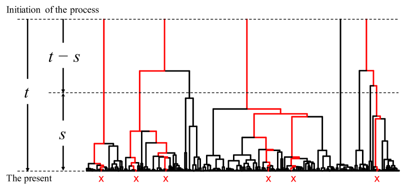
Figure 2: Number of ancestors of a sample of size $n$, $A_{n}(s;t)$, at time $t-s$. In this example, the number of ancestors of a sample of size $n=6$, shown in red, is $A_{6}(s,t)=4$. The number of ancestors of the entire population is $A_{\infty}(s;t)=8$.

3.1 Population Coalescence

Our initial aim is to calculate the distribution of $A_{\infty}(s;t)$. We begin with the following definition.

Definition 1.

[21, p378] If $N\sim\text{Pois}(\nu)$ is a Poisson random variable with mean $\nu$ and probability generating function (pgf) $G_{N}(z)=e^{-\nu(1-z)}$ and $M_{i}\sim\text{ShiftedGeom}(p)$, $0\leq p\leq 1$, $i=1,2,\ldots$, are i.i.d. shifted geometric random variables, independent of $N$, with common probability function $\mathbb{P}(M=m)=(1-p)p^{m-1}$, $m=1,2,\ldots$ and pgf $G_{M}(z)=(1-p)z(1-pz)^{-1}$, then the random variable

$$Q=\sum_{i=0}^{N}M_{i},$$

where $M_{0}:=0$, is said to be a geometric compound Poisson or Pólya-Aeppli random variable with parameters $(\nu,p)$.

The range of $Q$ is $\{0,1,2,\ldots\}$, with $\mathbb{P}(Q=0)=\mathbb{P}(N=0)=e^{-\nu}$. The corresponding pgf is

$$G_{Q}(z)=G_{N}(G_{M}(z))=\exp\left\{-\nu\frac{1-z}{1-pz}\right\}.$$ (13)

Theorem 1.

$A_{\infty}(s;t)$ is a Pólya-Aeppli random variable with parameters

$$\nu=x_{0}\mu(t;\alpha)=\frac{2\alpha x_{0}e^{\alpha t}}{e^{\alpha t}-1},\qquad p=p(s,t;\alpha)=\frac{e^{\alpha s}-e^{\alpha t}}{1-e^{\alpha t}}.$$ (14)

Proof.

Noting from Eq. (11) that, conditional on a scaled population $x$ at a time $s$ in the past, the number of families descendant from founder lineages at $t-s$ is Poisson with mean $x\mu(s;\alpha)$,

$$\mathbb{P}\left(A_{\infty}(s;t)=k\right) = \int_{0}^{\infty}\mathbb{P}\left(A_{\infty}(s;t)=k,X(t-s)\in(x,x+dx)\right)$$

$$= \int_{0}^{\infty}\mathcal{P}\left(k;x\mu(s;\alpha)\right)f_{X(t-s)}(x;\alpha,x_{0})dx.$$

The pgf of $A_{\infty}(s;t)$ is, from Eq. (12),

$$G_{A_{\infty}(s;t)}(z) = \int_{0}^{\infty}e^{-\mu(s;\alpha)x(1-z)}f_{X(t-s)}(x;\alpha,x_{0})dx$$

$$= \psi(\mu(s;\alpha)(1-z),t-s;\alpha,x_{0})$$

$$= \exp\left\{-\frac{\mu(s;\alpha)(1-z)x_{0}\mu(t-s;\alpha)\beta(t-s;\alpha)}{1+\mu(s;\alpha)(1-z)\beta(t-s;\alpha)}\right\}$$

$$= \exp\left\{\frac{2\alpha x_{0}e^{\alpha t}(1-z)}{1-e^{\alpha s}+(e^{\alpha s}-e^{\alpha t})(1-z)}\right\}$$

$$= \exp\left\{-x_{0}\mu(t;\alpha)\frac{1-z}{1-p(s,t;\alpha)z}\right\},$$

which is of the form of Eq. (13). ∎

It will be convenient below to consider the pgf of $A_{\infty}(s;t)$ conditional on $X(t)>0$, i.e. on survival of the population at time $t$. An equivalent condition is $A_{\infty}(s;t)>0$ since the population at time $t$ is not extinct if and only if it has ancestors at time $t-s$. Since the pgf of any random variable $Q$ with range $\{0,1,2,\ldots\}$ is $G_{Q}(z)=\sum_{n=0}^{\infty}\mathbb{P}(Q=n)z^{n}$, the pgf of $Q$ conditioned on $Q>0$ is

$$G_{Q\mid Q>0}(z)=\sum_{n=1}^{\infty}\mathbb{P}(Q=n\mid Q>0)z^{n}=\frac{G_{Q}(z)-G_{Q}(0)}{1-G_{Q}(0)}.$$

Hence

$$G_{A_{\infty}(s;t)\mid X(t)>0}(z) = G_{A_{\infty}(s;t)\mid A_{\infty}(s;t)>0}(z)$$

$$= \frac{G_{A_{\infty}(s;t)}(z)-G_{A_{\infty}(s;t)}(0)}{1-G_{A_{\infty}(s;t)}(0)}$$

$$= \frac{\exp\left\{-x_{0}\mu(t;\alpha)\frac{1-z}{1-p(s,t;\alpha)z}\right\}-\exp\left\{-x_{0}\mu(t;\alpha)\right\}}{1-\exp\left\{-x_{0}\mu(t;\alpha)\right\}}.$$

3.2 Sample Coalescence

To calculate the coalescent distribution for a sample of size $n$ in terms of the coalescent distribution of the population we begin with the following lemma.

Lemma 1.

Conditional on $A_{\infty}(s;t)=k>0$, the probability that a sample of size $n>0$ taken at time $t$ has $j\leq k$ ancestors at time $t-s$ is

$$\mathbb{P}(A_{n}(s;t)=j\mid A_{\infty}(s;t)=k)={k\choose j}\frac{n!}{k_{(n)}}{n-1\choose j-1},\qquad 1\leq j\leq k,$$

where $k_{(n)}=k(k+1)\cdots(k+n-1)$ is the rising factorial. The distribution of $A_{n}(s;t)$ conditional on $A_{\infty}(s;t)$ is independent of the total population size at $t$.

Proof.

Since at a given time each family size within the population descended from an individual is i.i.d. exponentially distributed, the distribution of relative family sizes of the population at time $t$ descended from the $k$ ancestors at time $t-s$ is Dirichlet$(\mathbf{1}_{k})$, where the vector $\mathbf{1}_{k}=(1,\ldots,1)$ has $k$ entries, independent of the total population size. Hence the distribution of family sizes $(N_{1},\ldots,N_{k})$ in a sample of size $n$ is Dirichlet-multinomial$(n,\mathbf{1}_{k})$ [20, p80],

$$\mathbb{P}(\mathbf{N}=\mathbf{n}\mid A_{\infty}(s;t)=k)=\frac{n!}{k_{(n)}}.$$

This is a uniform distribution over the simplicial lattice $\{n_{1},\ldots,n_{k}\geq 0:\sum_{i=1}^{k}n_{i}=n\}$. Any point $(n_{1},\ldots,n_{k})$ in this lattice corresponding to exactly $j$ ancestors has $j$ non-zero components and $n-j$ zero components, with the non-zero components summing to $n$. Thus the number of points in this lattice corresponding to $j$ ancestors is the number of ways of choosing the $j$ ancestors from $k$, times the number of points in the simplicial lattice $\{n_{1},\ldots,n_{j}>0:\sum_{i=1}^{j}n_{i}=n\}$, that is,

$${k\choose j}\times{n-1\choose j-1},$$

and the result follows. ∎

Theorem 2.

In a sample of size $n>0$ taken at time $t$, the distribution of the number of ancestors at time $t-s$ is

$$\mathbb{P}(A_{n}(s;t)=j)$$

$$= n!{n-1\choose j-1}\sum_{k=j}^{\infty}{k\choose j}\frac{1}{k_{(n)}}\mathbb{P}\left(A_{\infty}(s;t)=k\mid A_{\infty}(s;t)>0\right),\quad j=1,2,\ldots,n.$$

Proof.

Because the sample size $n$ is assumed to be strictly positive, so the number of ancestors of the entire population at time $t-s$ must also be strictly positive. Equivalently, conditioning on $A_{\infty}(s;t)>0$ has no effect on the probability of the event $A_{n}(s;t)=j$. Then from Lemma 1, for $1\leq j\leq k$ and $0<n<\infty$ we have the joint distribution

$$\mathbb{P}(A_{n}(s;t)=j,A_{\infty}(s;t)=k)$$

$$= \mathbb{P}(A_{n}(s;t)=j,A_{\infty}(s;t)=k\mid A_{\infty}(s;t)>0)$$

$$= \mathbb{P}(A_{n}(s;t)=j\mid A_{\infty}(s;t)=k)\mathbb{P}(A_{\infty}(s;t)=k\mid A_{\infty}(s;t)>0)$$

$$= n!{n-1\choose j-1}{k\choose j}\frac{1}{k_{(n)}}\mathbb{P}(A_{\infty}(s;t)=k\mid A_{\infty}(s;t)>0).$$

Note that the conditioning $A_{\infty}(s;t)>0$ in this proof is essential to ensure that the joint distribution is correctly normalised: The range of $A_{\infty}(s;t)$ includes zero, corresponding to extinction of the population, whereas the range of $A_{n}(s;t)$ for $n>0$, does not include zero. Since $A_{\infty}(s;t)\geq A_{n}(s;t)>0$, the event $A_{\infty}(s;t)=0$ must be excluded. Summing over $k\geq j$ then gives the required marginal distribution of $A_{n}(s;t)$. ∎

4 Coalescence at fixed $s$ as $t\to\infty$: subcritical case

The asymptotic limit as $t\to\infty$ of a subcritical branching process conditioned on survival of the population is known as the quasi-stationary limit [24]. Noting that for $\alpha<0$,

$$\lim_{t\to\infty}\mu(t;\alpha)=0,\qquad\lim_{t\to\infty}p(s,t;\alpha)=e^{-|\alpha|s},$$

the pgf of the number of ancestors $A_{\infty}(s;t)$ of the population at time $s$ back in the quasi-stationary limit is, from Eq. (3.1),

$$\lim_{t\to\infty}G_{A_{\infty}(s;t)\mid A_{\infty}(s;t)>0}(z)=\frac{(1-e^{-|\alpha|s})z}{1-ze^{-|\alpha|s}}.$$

This is the pgf of a shifted geometric distribution,

$$\lim_{t\to\infty}\mathbb{P}(A_{\infty}(s;t)=k\mid A_{\infty}(s;t)>0)=(1-e^{-|\alpha|s})e^{-|\alpha|(k-1)s},\qquad k=1,2,\ldots.$$ (17)

Let $\{W_{j}\}_{j=2}^{\infty}$ be the quasi-stationary inter-coalescent waiting times when the population has $j$ ancestors, and let $T_{k}=\sum_{j=k}^{\infty}W_{j}$ be the time back to when there are first $k-1$ ancestors (see Fig. 3). Then

$$\mathbb{P}(T_{k}>s) = \lim_{t\to\infty}\mathbb{P}(A_{\infty}(s;t)\geq k\mid A_{\infty}(s;t)>0)$$

$$= \sum_{j=k}^{\infty}(1-e^{-|\alpha|s})e^{-|\alpha|(j-1)s}$$

$$= e^{-|\alpha|(k-1)s}.$$

Thus $T_{k}$ has an exponential distribution with rate $|\alpha|(k-1)$ and mean $1/(|\alpha|(k-1))$. The mean coalescence times

$$\mathbb{E}\big{[}W_{k}\big{]}=\mathbb{E}\big{[}T_{k}-T_{k+1}]=\frac{1}{|\alpha|k(k-1)},$$

are the same as in the Kingman coalescent apart from scale. If a mutation occurs while $k$ ancestors then the mutant relative frequency $U$ in the population is Beta $(1,k-1)$ with density $(k-1)(1-u)^{k-2},\>u\in(0,1)$.

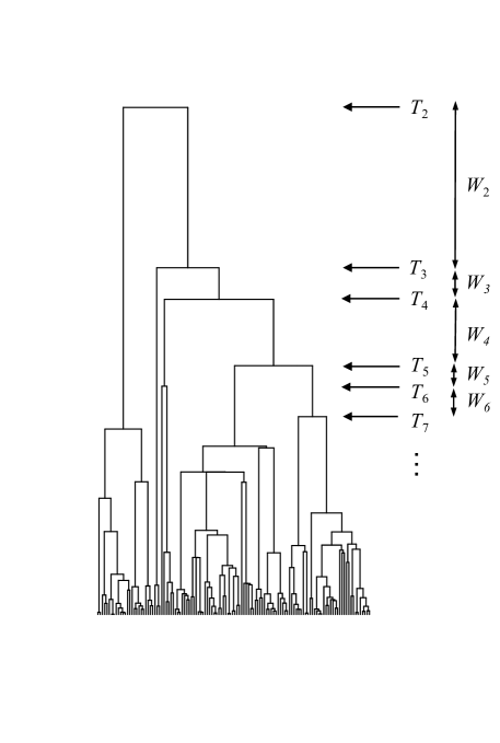
Figure 3: Coalescent times $T_{n}$ measured back from the present, and inter-coalescent times $W_{n}=T_{n}-T_{n+1}$.

4.1 Quasi-stationary subcritical sample coalescent

Substituting Eq. (17) into Eq. (2) gives

$$\mathbb{P}(A_{n}(s;\infty)=j)=n!{n-1\choose j-1}\sum_{k=j}^{\infty}{k\choose j}\frac{1}{k_{(n)}}(1-e^{-|\alpha|s})e^{-|\alpha|(k-1)s}.$$

Writing

$$\frac{1}{k_{(n)}}=\frac{(k-1)!}{(k+n-1)!}=\frac{1}{(n-1)!}\cdot B(k,n)=\frac{1}{(n-1)!}\int_{0}^{1}u^{k-1}(1-u)^{n-1}du,$$

we have

$$\mathbb{P}(A_{n}(s;\infty)=j)$$ (18)

$$= n{n-1\choose j-1}\sum_{k=j}^{\infty}{k\choose j}\int_{0}^{1}u^{k-1}(1-u)^{n-1}du\cdot(1-e^{-|\alpha|s})e^{-(k-1)|\alpha|s}$$

$$= n{n-1\choose j-1}(1-e^{-|\alpha|s})\int_{0}^{1}\frac{e^{-(j-1)|\alpha|s}}{(1-ue^{-|\alpha|s})^{j+1}}u^{j-1}(1-u)^{n-1}du.$$

We are interested in the expected sample inter-coalescent waiting times. Begin with the integral

$$\mathcal{I}_{j}(u)=\int_{0}^{\infty}(1-e^{-|\alpha|s})\frac{e^{-(j-1)|\alpha|s}}{(1-ue^{-|\alpha|s})^{j+1}}ds=\frac{1}{|\alpha|j(j-1)(1-u)^{j-1}},$$

which follows from induction by checking that $\mathcal{I}_{2}(u)=\{2|\alpha|(1-u)\}^{-1}$ and $\mathcal{I}_{j+1}(u)=(j+1)^{-1}\mathcal{I}_{j}^{\prime}(u)$. Then

$$\mathbb{E}\left[W_{j}\right] = \mathbb{E}[T_{j}-T_{j+1}]$$

$$= \int_{0}^{\infty}\{\mathbb{P}(T_{j}>s)-\mathbb{P}(T_{j+1}>s)\}ds$$

$$= \int_{0}^{\infty}\{\mathbb{P}(A_{n}(s;\infty)\geq j)-\mathbb{P}(A_{n}(s;\infty)\geq j+1)\}ds$$

$$= \int_{0}^{\infty}\mathbb{P}\left(A_{n}(s;\infty)=j\right)ds$$

$$= n{n-1\choose j-1}\frac{1}{|\alpha|j(j-1)}\int_{0}^{1}u^{j-1}(1-u)^{n-j}du$$

$$= n{n-1\choose j-1}\frac{1}{|\alpha|j(j-1)}B(j,n-j+1)$$

$$= \frac{1}{|\alpha|j(j-1)}.$$

Once again this leads to the same expected waiting times as the Kingman coalescent, up to a scale. If neutral mutations between multiple alleles are included, in the limit of small mutation rates these waiting times lead to an identical distribution as that for a neutral stationary Wright-Fisher population [5, Theorem 1]. This equivalence has also been discovered by Burden and Griffiths [6, Corollary 1] using Laplace transform methods.

In addition to its expectation, one can also deduce the distribution of $W_{k}=T_{k}-T_{k+1}$. Consider, with notation $w_{k}=t_{k}-t_{k+1}$,

$$\mathbb{P}(T_{k}>t_{k}\mid T_{k+1}=t_{k+1})=\mathbb{P}(A_{k}(W_{k},\infty)=k)$$

$$= k(1-e^{-|\alpha|w_{k}})\int_{0}^{1}\frac{e^{-|\alpha|(k-1)w_{k}}}{(1-ue^{-|\alpha|w_{k}})^{k+1}}u^{k-1}(1-u)^{k-1}du,$$

by substituting $s=w_{k}$, $n=j=l$ in Eq, (18). Since the conditional distribution does not depend on $t_{k+1}$,

$$\mathbb{P}(W_{k}>w)=k(1-e^{-|\alpha|w})\int_{0}^{1}\frac{e^{-|\alpha|(k-1)w}}{(1-ue^{-|\alpha|w})^{k+1}}u^{k-1}(1-u)^{k-1}du,$$

which differs from the exponential distribution waiting time for a Kingman coalescent. The formula applies both to the coalescent tree of the entire population and to the coalescent tree of a finite sample.

5 Population coalescence at fixed $t$ as $s\to 0$

Recall from Theorem 1 that the number of ancestors at time $t-s$ of the population at time $t$ follows a Pólya-Aeppli distribution, that is, the sum of a Poisson number of independent geometric random variables. Write

$$A_{\infty}(s;t)=\sum_{j=0}^{N(t)}M_{j}(s,t),$$

where $N(t)\sim\text{Pois}(x_{0}\mu(t;\alpha))$, $M_{j}(s,t)\sim\text{ShiftedGeom}(p(s,t))$, $j=1,2,\ldots$ with $p(s,t)$, defined by Eq. (14), are independent, and $M_{0}(s,t):=0$. The interpretation of Theorem 1 is that $N(t)$ is the number of founders at time $0$ of the entire population at time $t$, and $M_{j}(s,t)$ is the number of descendants of the $j$th founder alive at time $t-s$. For example, in the instance shown in Fig. 2, $N(t)=5$ and $(M_{1}(s,t),\ldots,M_{5}(s,t))=(1,2,1,1,3)$. Note that $M_{j}(s,t)>0$ for $j>0$ since the ancestral line of every member of the population at time $t$ passes through $t-s$ and that $A_{\infty}(s;t)=0$ if and only if the population is extinct at time $t$.

We next demonstrate that $M_{j}(s,t)$ can also be interpreted as a count of the descendants of a linear BD process with a single founder, conditioned on non-extinction. Consider a linear BD process $\{M(u)\}_{u\geq 0}$ with a single founder, $M(0)=1$, birth rate $\hat{\lambda}$, and death rate $\hat{\mu}$, and transition probabilities as defined in Eq. (4). Then Feller [15, p480] shows that

$$\mathbb{P}(M(u)=m)=\begin{cases}\hat{\mu}B(u)&m=0\\ (1-\hat{\lambda}B(u))(1-\hat{\mu}B(u))(\hat{\lambda}B(u))^{m-1}&m=1,2,\ldots,\end{cases}$$

where

$$B(u)=\frac{1-e^{(\hat{\lambda}-\hat{\mu})u}}{\hat{\mu}-\hat{\lambda}e^{(\hat{\lambda}-\hat{\mu})u}}.$$

Conditional on non-extinction of the process up to time $u$,

$$\mathbb{P}(M(u)=m\mid M(u)>0)=(1-\hat{\lambda}B(u))(\hat{\lambda}B(u))^{m-1},\qquad m=1,2,\ldots,$$

and so $(M(u)\mid M(u)>0)\sim\text{ShiftedGeom}(\hat{\lambda}B(u))$. Equating $\hat{\lambda}B(t-s)$ with $p(s,t;\alpha)$ defined by Eq. (14) at fixed $t$ gives

$$\hat{\lambda}-\hat{\mu}=\alpha,\qquad\frac{\hat{\mu}}{\hat{\lambda}}=e^{-\alpha s},$$

or

$$\hat{\lambda}(s)=\frac{\alpha}{1-e^{-\alpha s}},\qquad\hat{\mu}(s)=\frac{\alpha e^{-\alpha s}}{1-e^{-\alpha s}}.$$ (19)

Nee et al. [25] define the reconstructed process (RP) of a linear BD process with birth rate $\hat{\lambda}$ and death rate $\hat{\mu}$ stopped at time $T$ after initiation to be the time-inhomogeneous pure-birth process constructed by pruning lineages which have not survived to time $T$. Denote by $\mathcal{RP}(T,\hat{\lambda},\hat{\mu})$ the set of RPs for a given $T$, $\hat{\lambda}$ and $\hat{\mu}$. Elements of this set differ by their initial conditions $M(0)$. With this definition we have the following lemma, illustrated in Fig. 4.

Lemma 2.

For any $0<s<t$, that part of the coalescent tree of a parameter-$\alpha$ Feller diffusion $\{X(u)\}_{0\leq u\leq t}$ lying within the interval $[0,t-s]$ is generated by a process in $\mathcal{RP}(t-s,\hat{\lambda}(s),\hat{\mu}(s))$, where $\hat{\lambda}(s)$ and $\hat{\mu}(s)$ are defined by Eq. (19).

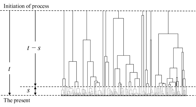
Figure 4: Illustration of Lemma 2: That part of the coalescent tree of the Feller diffusion $\{X(u)\}_{0\leq u\leq t}$ lying in the interval $[0,t-s]$ is generated by an element of $\mathcal{RP}(t-s,\hat{\lambda}(s),\hat{\mu}(s))$.

Proof.

The inhomogeneous birth rate of any process in $\mathcal{RP}(T,\hat{\lambda},\hat{\mu})$ at time $u$ since initiation is equal to [19, Eq. (1.5)]

$$\lambda^{\rm eff}(u;T,\lambda,\mu)$$

$$= \hat{\lambda}\times\mathbb{P}(\text{a single lineage born at time $u$ is not extinct by time $T$})$$

$$= \hat{\lambda}\times(1-\hat{\mu}B(u))$$

$$= \hat{\lambda}\times\frac{\hat{\lambda}-\hat{\mu}}{\hat{\lambda}-\hat{\mu}e^{-(\hat{\lambda}-\hat{\mu})(T-u)}},\qquad 0\leq u\leq T.$$

Substituting $t-s$ for $T$ and Eq. (19) for $\hat{\lambda}$ and $\hat{\mu}$, the inhomogeneous birth rate for any process in $\mathcal{RP}(t-s,\hat{\lambda}(s),\hat{\mu}(s))$ is

$$\lambda^{\rm eff}(u;t-s,\hat{\lambda}(s),\hat{\mu}(s)) = \frac{\hat{\lambda}(s)-\hat{\mu}(s)}{1-(\hat{\mu}(s)/\hat{\lambda}(s))e^{-(\hat{\lambda}(s)-\hat{\mu}(s))(t-s-u)}}$$ (20)

$$= \frac{\alpha}{1-e^{-\alpha(t-u)}},\qquad 0\leq u\leq t-s.$$

The important point to note is that this inhomogeneous birth rate does not depend on $s$, and hence elements of the set of reconstructed processes $\{\mathcal{RP}(t-s,\hat{\lambda}(s),\hat{\mu}(s)):0\leq s<t\}$ differ only to the extent that we choose to stop the processes at different times $s$ short of the limiting time $t$. Since the running parameters $\hat{\lambda}(s)$ and $\hat{\mu}(s)$ are constructed from a process which generates as its RP the number of ancestors $A_{\infty}(t-u,t)$ of the entire population of a Feller diffusion with parameter $\alpha$, the result follows. ∎

We are now in a position to construct the coalescent tree of a Feller diffusion as the limiting case of the RP of a linear BD process.

Theorem 3.

The coalescent tree of a Feller diffusion with parameter $\alpha$, observed at time $t$ since initiation, is a time-inhomogeneous pure-birth process with birth rate at time $u$ since initiation equal to

$$\lambda^{\rm coal}(u;t):=\frac{\alpha}{1-e^{-\alpha(t-u)}},\qquad 0\leq u<t.$$

Proof.

Consider the limit $s\to 0$ in Fig. (4). From Eq. (19),

$$\hat{\lambda}(s)=s^{-1}+\tfrac{1}{2}\alpha+\mathcal{O}(s),\quad\hat{\mu}(s)=s^{-1}-\tfrac{1}{2}\alpha+\mathcal{O}(s),\qquad\text{as }s\to 0.$$

Identify $\tfrac{1}{2}s$ with $\epsilon$ in Proposition 1 and define a random variable

$$X_{s}(t)=\tfrac{1}{2}sM(t-s),$$ (21)

where $\{M(u)\}_{0\leq u\leq t-s}$ is a birth-death process with rates $\hat{\lambda}(s)$, $\hat{\mu}(s)$. Then as $s\to 0$ the limiting generator of the process $X_{s}(t)$ is that of a Feller diffusion with parameter $\alpha$. The required result then follows immediately from Lemma 2 and that $\lambda^{\rm coal}(u;t)=\lambda^{\rm eff}(u;t-s,\hat{\lambda}(s),\hat{\mu}(s))$ is independent of $s$. ∎

In the context of population genetics, the Feller diffusion is usually approached as a limit of a BGW process as described in Section 2.2. The above procedure provides an alternative view in terms of that part of the population’s coalescent tree at times earlier than $t-s$. As $s\to 0$ the effective birth rate $\lambda^{\rm coal}(t-s;t)\to\infty$, consistent with the coalescent tree “coming down from infinity”. The running parameters $\hat{\lambda}(s)$, $\hat{\mu}(s)$ also become infinite as $s\to 0$ while their difference $\alpha$ remains fixed. Thus a Feller diffusion can be seen as the limit of a linear BD process in which births and deaths occur at an arbitrary high rate.

It remains to match the scale $s$ of the BD limit with the scale $y_{0}$ and parameters $\log\lambda$ and $\sigma^{2}$ of the BGW limit in such a way that the limiting process is the same Feller diffusion for both limits. From Eqs. (5), (6) and (21) we have

$$\tfrac{1}{2}s=\frac{1}{y_{0}}=\frac{\log\lambda}{\alpha\sigma^{2}}.$$ (22)

Implicit in this matching is the notion that the ancestry of a large-population, near-critical BGW process is well approximated by the coalescent tree of the corresponding linear BD process.

6 The coalescent tree of a super-critical Feller diffusion as a reversed reconstructed process

[17] and [19] generate the coalescent tree of a supercritical linear BD process as a RRP. The RRP is an inhomogeneous pure-death process which runs backwards in time from the present tracing the ancestral coalescent tree. Construction of the RRP from a BD process consists of first constructing the RP for a fixed time since initiation with a single ancestor, and then imposing an improper uniform prior on the time since initiation and conditioning on the present number of leaves [2, 28]. By effecting a time rescaling of the RRP to a rate-1 pure-death Yule process,  [19] reproduce earlier results of Gernhard [17, Theorem 4.1] for the distribution of coalescent times for a supercritical BD process with constant birth and death rates.

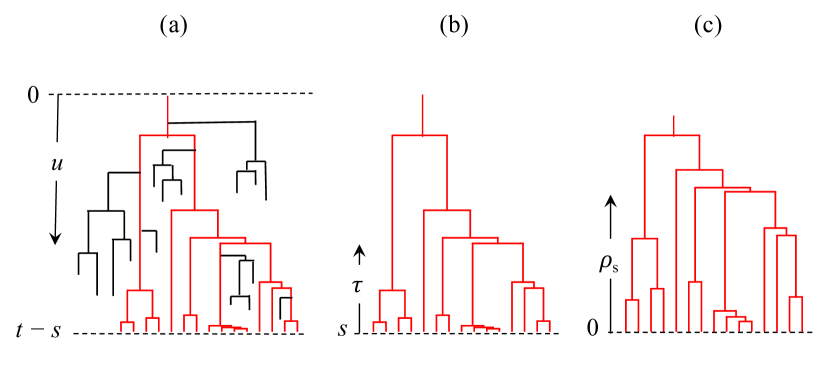
Figure 5: Construction of the RRP from the RP of a linear BD process, and subsequent mapping to a rate-1 pure death process: (a) a linear BD process process defined over the interval $0\leq u\leq t-s$, with the corresponding RP shown in red; (b) the constructed RRP over $s\leq\tau<\infty$; and (c) the corresponding rate-1 pure death process over the interval $0\leq\rho_{s}<\infty$.

Below we construct the coalescent tree for a super-critical Feller diffusion conditioned on $X(t)=x$ with an improper uniform prior on initiation of a process with a single ancestor. The construction is based on the $s\to 0$ limit of the RRP derived from the RP of a linear BD process on the interval $[0,t-s]$ with birth-rate $\hat{\lambda}(s)$ and death rate $\hat{\mu}(s)$. The RP of a linear BD process is represented in Fig 5(a). To construct the RRP represented in Fig. 5(b) we introduce a parameter $\tau=t-u$, $s\leq\tau<\infty$, measured backwards from a time $s$ in the past before the present and assume an improper uniform prior on the time since initiation of the forward process. From Eq. (20), the effective death rate of this RRP is

$$\mu_{\rm eff}(\tau)=\frac{\alpha}{1-e^{-\alpha\tau}},\qquad s\leq\tau<\infty.$$

The RRP is conditioned on a boundary at $\tau=s$ and is allowed to run backwards until the birth of the earliest ancestor.

Following Ignatieva et al. [19, Section 2.1], the inhomogeneous pure-death process can be mapped onto a time-reversed rate-1 Yule process, represented in Fig 5(c). To this end, define a rescaled time $\rho_{s}(\tau)$ such that, if the random variable $T$ is the time of death of an individual reversed lineage starting at time $s$, then $\mathbb{P}(T>\tau)=e^{-\rho_{s}(\tau)}$ for $\tau\geq s$ and $e^{\rho_{s}(s)}=1$. Thus

$$\mu_{\rm eff}(\tau)d\tau=\frac{\mathbb{P}(\tau\leq T<\tau+d\tau)}{\mathbb{P}(T\geq\tau)}=\frac{e^{-\rho_{s}(\tau)}-e^{-\rho_{s}(\tau+d\tau)}}{e^{-\rho_{s}(\tau)}}=\rho_{s}^{\prime}(\tau)d\tau,$$

which, together with the initial condition gives

$$\rho_{s}(\tau)=\int_{s}^{\tau}\mu_{\rm eff}(\xi)d\xi=\int_{s}^{\tau}\frac{\alpha e^{\alpha\xi}}{e^{\alpha\xi}-1}d\xi=\log\frac{e^{\alpha\tau}-1}{e^{\alpha s}-1}.$$

The mapping to a rate-1 Yule process inverts to

$$\alpha\tau=\log\left(1+(e^{\alpha s}-1)e^{\rho_{s}}\right),\qquad 0\leq\rho_{s}<\infty.$$ (23)

As an aside we note that the transformation to $\rho_{s}(\tau)$ accords with a remark of O’Connell [26, p425] regarding the limit of a near-critical continuous-time BGW process, once differences in notation and scaling, namely setting $\tau$ to unity and replacing $(\tau-s)/\tau$ with O’Connell’s $r$, are accounted for. A similar time change also appears in Harris et al. [18, below Eq. (4)].

Implicit in the above construction is an assumption that the RRP converges to a single ancestor. For the sub-critical case, $\alpha=\hat{\lambda}(s)-\hat{\mu}(s)<0$, one has that

$$\lim_{\tau\to\infty}\mathbb{P}(T>\tau)=\lim_{\tau\to\infty}e^{-\rho_{s}(\tau)}=1-e^{-|\alpha|s},$$

and there is a finite probability that an ancestral lines will never converge. For this reason the above construction only applies for the super-critical case $\alpha>0$.

It would be nice to dispense with the scale $s$ at this point by sending it to zero, but this entails beginning the time-reversed Yule process with an infinite number of particles at an infinite time in the past. This is a manifestation of the effect that the coalescent tree of a diffusion process comes down from infinity. However, recall from Eq. (22) that the scale $s$ also has meaning in terms of the BGW process underlying the Feller diffusion limit. With this interpretation, the parameter $\alpha$ and currently observed scaled population $X=x$ are related to the current (assumed arbitrarily large) physical population $M=y$ of an underlying BGW process with mean and variance $\lambda$ and $\sigma^{2}$ of the number of offspring per generation via Eqs. (21) and (22) by

$$x=\tfrac{1}{2}sy=\frac{\log\lambda}{\alpha\sigma^{2}}y.$$ (24)

Note that the initial conditions of the Feller diffusion process have been subsumed into the uniform prior on the time since initiation of the ancestral tree.

Figure 6 shows (a) a plot of a rate-1 pure death process and (b) the same tree mapped from the timescale $\rho_{s}$ onto the timescale $\alpha\tau$. This is a coalescent tree of the entire population with the branches over the recent short interval $0\leq\tau<s$ truncated.

Figure 6: (a) Tree constructed from a rate-1 pure-death process in time $\rho_{s}$ starting with $500$ leaves at time $\rho_{s}=0$, and (b) the corresponding reverse-reconstructed tree mapped from the time scale $\rho_{s}$ onto a time scale $\alpha\tau$ for $\tau>s$ using Eq. (23) with $\alpha s=0.001$.

7 Coalescent times in the RRP of a super-critical Feller diffusion

The following theorem gives the distribution of coalescent times as defined in Fig. 3 and of the number of ancestors at time $\tau$ before present.

Theorem 4.

Let $\cdots<T_{j}<\cdots<T_{3}<T_{2}<T_{1}$ be coalescence times in the coalescent tree of the reverse reconstructed process of a super-critical Feller diffusion beginning with population size $x$. The coalescent tree is assumed to be extended back in time so that there is a single ancestor. Then the coalescence times are distributed as a non-homogeneous Poisson process back in time with rate $\frac{d}{d\tau}\{-x/\beta(\tau)\}$, where $\beta(\tau)$ is defined by Eq. (8), and

$$\mathbb{P}\left(N(\tau)=j\right)=\frac{1}{j!}\left(\frac{x}{\beta(\tau)}\right)^{j}\exp\left\{-\frac{x}{\beta(\tau)}\right\},\>\tau>0,\ j=1,2,\ldots,$$ (25)

where $N(\tau)$ is be the number of ancestors at time $\tau$ back.

Proof.

Suppose that the current time is $t$ from the initiation of the population with one founder. We argue conditional on $M(t-s)=m$ where $\{M(u)\}_{0\leq u\leq t-s}$ is the RP in Fig. 5(a), then let $m\to\infty,s\to 0,\frac{1}{2}sm=x$, conditioning on the diffusion population size at $t$ being $x$ in the limit. Coalescent times before taking the limit form a reverse Markov chain with

$$\mathbb{P}\left(T_{j}>\tau_{j}\mid T_{j+1}=\tau_{j+1}\right) = \exp\left\{-j\int_{\tau_{j+1}}^{\tau_{j}}\mu_{\text{eff}}(\xi)d\xi\right\}$$ (26)

$$= \exp\left\{-j\log\left(\frac{e^{\alpha\tau_{j}}-1}{e^{\alpha\tau_{j+1}}-1}\right)\right\}$$

$$= \left(\frac{e^{\alpha\tau_{j+1}}-1}{e^{\alpha\tau_{j}}-1}\right)^{j},\ j=m-1,\ldots,1$$

$$\mathbb{P}\left(T_{m}>\tau_{m}\right) = \left(\frac{e^{\alpha s}-1}{e^{\alpha\tau_{m}}-1}\right)^{m},\ \tau_{m}>s.$$ (27)

The distribution of $T_{j}$ given $T_{j+1}=\tau_{j+1}$ is seen to be that of the minimum of $j$ independent random variables with distribution function $F$ such that

$$1-F_{\tau_{j+1}}(\tau)=\frac{e^{\alpha\tau_{j+1}}-1}{e^{\alpha\tau}-1},\quad\tau>\tau_{j+1}.$$

That is, $T_{m},T_{m-1},\ldots T_{1}$ are distributed as order statistics from small to large in an independent sample of $m$ from a distribution with

$$1-F(\tau)=\frac{e^{\alpha s}-1}{e^{\alpha\tau}-1},\quad\tau>s,$$

and corresponding density

$$f(\tau)=\frac{\alpha e^{\alpha\tau}(e^{\alpha s}-1)}{(e^{\alpha\tau}-1)^{2}},\quad\tau>s,$$

because

$$\mathbb{P}\left(T_{j}>\tau_{j}\mid T_{j+1}=\tau_{j+1}\right)=\left(\frac{1-F(\tau_{j})}{1-F(\tau_{j+1})}\right)^{j},$$

agreeing with (26). This is the probability that there are $j$ sample points larger than $\tau_{j}$ in the distribution truncated below at $\tau_{j+1}$. The dependence in $s$ appears in the distribution of $T_{m}$ in (27). Consider the pre-limit density of the $r$ maximal points $T_{1}>T_{2}>\cdots>T_{r}$ for fixed $r$,

$$\frac{m!}{(m-r)!}f(\tau_{1})\cdots f(\tau_{t})F(\tau_{r})^{m-r},\ \tau_{1}>\tau_{2}>\cdots>\tau_{r}.$$

Now

$$mf(\tau)\to\frac{2x\alpha^{2}e^{\alpha\tau}}{(e^{\alpha\tau}-1)^{2}}=\frac{d}{d\tau}\left(\frac{-x}{\beta(\tau)}\right),$$

and

$$F(\tau)^{m-r}\to\exp\left\{-\frac{2\alpha x}{e^{\alpha\tau}-1}\right\}=\exp\left\{\frac{-x}{\beta(\tau)}\right\}.$$

The limit density of $T_{1},\ldots,T_{r}$ is therefore

$$\left(\prod_{j=1}^{r}\frac{d}{d\tau_{j}}\left\{\frac{-x}{\beta(\tau_{j})}\right\}\right)\exp\left\{\frac{-x}{\beta(\tau_{r})}\right\},\quad\tau_{1}>\tau_{2}>\cdots>\tau_{r}>0.$$

These are finite-dimensional densities of points in the non-homogeneous Poisson process in the statement of the theorem, so the proof is completed. The Poisson distribution (25) follows, however it can be argued directly. In the pre-limit the probability that in a sample of $m$ there are $m-j$ points less than $\tau$ and $j$ points greater than $\tau$ is

$${m\choose j}\left(1-F(\tau)\right)^{j}F(\tau)^{m-j}$$

whose limit is Eq. (25).

∎

Corollary 1.

Let $N_{n}(\tau)$ be the number of ancestors of a sample of $n$ taken from a super-critical Feller diffusion with current population size $x$. The coalescent tree of the sample is assumed to be extended back in time so that there is a single ancestor. Then for $j=n,n-1,\ldots,1$

$$\mathbb{P}\left(N_{n}(\tau)=j\right) = \frac{n_{[j]}}{n_{(j)}j!}\left(\frac{x}{\beta(\tau)}\right)^{j}\exp\left\{-\frac{x}{\beta(\tau)}\right\}M\left(j,j+n,\frac{x}{\beta(\tau)}\right)$$

$$= \frac{1}{(j-1)!}{n\choose j}\left(\frac{x}{\beta(\tau)}\right)^{j}\int_{0}^{1}\exp\left\{-(1-v)\frac{x}{\beta(\tau)}\right\}v^{j-1}(1-v)^{n-1}dv,$$

where $M$ is Kummer’s confluent hypergeometric function defined by [1, Eq. (13.1.2)]

$$M(a,b,z)=\sum_{k=0}^{\infty}\frac{a_{(k)}}{b_{(k)}}\frac{z^{k}}{k!}.$$

Let $\left\{W^{(n)}_{j}\right\}_{j=2}^{n}$ be the inter-coalescent times in a sample of $n$. The mean inter-coalescent times are

$$\mathbb{E}\left[W^{(n)}_{j}\right]=\frac{2(2\alpha)^{j-1}x^{j}}{(j-1)!}{n\choose j}\int_{0}^{1}v^{j-1}(1-v)^{n-1}\int_{0}^{\infty}\frac{u^{j-1}}{1+u}e^{-2\alpha x(1-v)u}dudv.$$ (29)

Proof.

From Lemma 1

$$\mathbb{P}(N_{n}(\tau)=j\mid N(\tau)=l)={l\choose j}\frac{n!}{l_{(n)}}{n-1\choose j-1},\qquad 1\leq j\leq l,$$ (30)

because $N_{n}(\tau)$ is independent of the total current population size $X$ conditional on $N_{\infty}(\tau)$. The distribution (30) also only depends on the ancestry at time $\tau$ back from present time, not on the fact that the process is initiated from one founder.

Then from Theorem 4 the unconditional probability

$$\mathbb{P}\left(N_{n}(\tau)=j\right) = \sum_{l=j}^{\infty}{l\choose j}\frac{n!}{l_{(n)}}{n-1\choose j-1}\frac{1}{l!}\left(\frac{x}{\beta(\tau)}\right)^{l}\exp\left\{-\frac{x}{\beta(\tau)}\right\}$$

$$= \frac{1}{j!}\left(\frac{x}{\beta(\tau)}\right)^{j}\exp\left\{-\frac{x}{\beta(\tau)}\right\}\frac{(n-1)!n!}{(n-j)!(n-1+j)!}$$

$$\quad\times\sum_{k=0}^{\infty}\frac{1}{k!}\left(\frac{x}{\beta(\tau)}\right)^{k}\frac{j_{(k)}}{(j+n)_{(k)}}$$

$$\equiv \frac{n_{[j]}}{n_{(j)}j!}\left(\frac{x}{\beta(\tau)}\right)^{j}\exp\left\{-\frac{x}{\beta(\tau)}\right\}M\left(j,j+n,\frac{x}{\beta(\tau)}\right),$$

where the summation shift $l=k+j$ has been used in the second line. The alternate integral form in Eq. (1) follows from

$$e^{-x/\beta(\tau)}\sum_{k=0}^{\infty}\frac{1}{k!}\left(\frac{x}{\beta(\tau)}\right)^{k}\frac{j_{(k)}}{(j+n)_{(k)}}$$

$$= e^{-x/\beta(\tau)}\sum_{k=0}^{\infty}\frac{1}{k!}\left(\frac{x}{\beta(\tau)}\right)^{k}\frac{B(j+k,n)}{B(j,n)}$$

$$= \frac{1}{B(j,n)}e^{-x/\beta(\tau)}\sum_{k=0}^{\infty}\frac{1}{k!}\left(\frac{x}{\beta(\tau)}\right)^{k}\int_{0}^{1}v^{j+k-1}(1-v)^{n-1}dv$$

$$= \frac{(j+n-1)!}{(j-1)!(n-1)!}\int_{0}^{1}e^{-(1-v)x/\beta(\tau)}v^{j+k-1}(1-v)^{n-1}dv.$$

The mean inter-coalescent times are

$$\mathbb{E}\left[W^{(n)}_{j}\right]=\int_{0}^{\infty}\mathbb{P}\left(N_{n}(\tau)=j\right)d\tau$$

which evaluates to Eq. (29) after change of integration variable

$$u=\frac{1}{2\alpha\beta(\tau)}=\frac{1}{e^{\alpha\tau}-1},\qquad\tau=\frac{1}{\alpha}\log\left(1+\frac{1}{u}\right),$$

$$d\tau=-\frac{1}{\alpha}\frac{du}{u(u+1)}$$

and some further simplification. ∎

8 Summary and Conclusions

The results of this paper hinge on the two key theorems of Section 3 which give formulae for the distribution of the number of ancestors at time $t-s$ of the population (Theorem 1) and of a uniform random sample of size $n$ (Theorem 2) from a Feller diffusion at a time $t$ since initiation of the process in terms of the parameter $\alpha$ of the diffusion and an initial condition $X(0)=x_{0}$. Two applications of these theorems are given. The first application is an efficient derivation of sample coalescent waiting times for the quasi-stationary subcritical Feller diffusion (Section 4).

In the second application the coalescent tree of a supercritical Feller diffusion is identified as the limit of the RP of a BD process with appropriately scaled birth and death rates (Theorem 3). The corresponding coalescent tree assuming a single ancestor is then used to calculate the distribution of coalescent times before the present time (Theorem 4) and to obtain a formula for expected coalescent times in the ancestry of a finite sample (Corollary 1).

With the intention of being of interest to the population genetics community, who are familiar with the [23] limit in which the population size is taken to infinity while generation times and mutation rates shrink to zero, we have taken the approach of treating the Feller diffusion primarily as the continuum limit of a discrete BGW process. The results of our theorems can be translated to all physically meaningful quantities in the underlying BGW process being approximated, including the mean $\lambda$ and variance $\sigma^{2}$ of the number of offspring per parent per generation, initial population counts at initiation of a BG process $m_{0}$ and $y_{0}$, and observed population counts at a later time $y$, via Eqs. (5), (6), and (24).

References

- Abramowitz and Stegun [1965] Abramowitz, M., Stegun, I.A., 1965. Handbook of mathematical functions: with formulas, graphs, and mathematical tables. Dover Publications, New York.
- Aldous and Popovic [2005] Aldous, D., Popovic, L., 2005. A critical branching process model for biodiversity. Advances in Applied Probability 37, 1094–1115.
- Athreya and Ney [1972] Athreya, K.B., Ney, P.E., 1972. Branching Processes. Springer Berlin Heidelberg. doi:10.1007/978-3-642-65371-1.
- Baake and Wakolbinger [2015] Baake, E., Wakolbinger, A., 2015. Feller’s contributions to mathematical biology, in: René L. Schilling, Zoran Vondraček, W.A.W. (Ed.), Selected Papers of William Feller. Springer. volume 1.
- Burden and Griffiths [2019] Burden, C., Griffiths, R., 2019. The stationary distribution of a sample from the Wright-Fisher diffusion model with general small mutation rates. Journal of Mathematical Biology 78, 1211–1224.
- Burden and Griffiths [2023] Burden, C.J., Griffiths, R.C., 2023. The stationary and quasi-stationary properties of neutral multi-type branching process diffusions. Stochastic Models 39, 185–218.
- Burden and Simon [2016] Burden, C.J., Simon, H., 2016. Genetic drift in populations governed by a Galton–Watson branching process. Theoretical Population Biology 109, 63–74.
- Burden and Soewongsono [2019] Burden, C.J., Soewongsono, A.C., 2019. Coalescence in the diffusion limit of a Bienaymé–Galton–Watson branching process. Theoretical Population Biology 130, 50–59.
- Cox and Miller [1978] Cox, D.R., Miller, H.D., 1978. The theory of stochastic proceesses. Chapman and Hall, London.
- Crespo et al. [2021] Crespo, F.F., Posada, D., Wiuf, C., 2021. Coalescent models derived from birth-death processes. Theoretical Population Biology 142, 1–11.
- Ewens [2004] Ewens, W.J., 2004. Mathematical population genetics. volume 27. 2nd ed ed., Springer, New York.
- Feller [1939] Feller, W., 1939. Die Grundlagen der Volterraschen Theorie des Kampfes Ums Dasein in Wahrscheinlichkeitstheoretischer Behandlung. Acta Biotheoretica 5, 11–40. doi:10.1007/bf01602932.
- Feller [1951a] Feller, W., 1951a. Diffusion processes in genetics, in: Proc. Second Berkeley Symp. Math. Statist. Prob, University of California Press, Berkeley. pp. 227–246.
- Feller [1951b] Feller, W., 1951b. Two singular diffusion problems. Annals of Mathematics 54, 173–182.
- Feller [1968] Feller, W., 1968. An introduction to probability theory and its applications.. volume 1. 3rd edition ed., Wiley & Sons, New York, N.Y.
- Gan and Waxman [2015] Gan, X., Waxman, D., 2015. Singular solution of the Feller diffusion equation via a spectral decomposition. Physical Review E 91, 012123.
- Gernhard [2008] Gernhard, T., 2008. The conditioned reconstructed process. Journal of Theoretical Biology 253, 769–778.
- Harris et al. [2020] Harris, S.C., Johnston, S.G., Roberts, M.I., 2020. The coalescent structure of continuous-time Galton-Watson trees. The Annals of Applied Probability 30, 1368–1414.
- Ignatieva et al. [2020] Ignatieva, A., Hein, J., Jenkins, P.A., 2020. A characterisation of the reconstructed birth-death process through time rescaling. Theoretical Population Biology 134, 61–76.
- Johnson et al. [1997] Johnson, N.L., Kotz, S., Balakrishnan, N., 1997. Discrete multivariate distributions. Wiley, New York, N.Y.
- Johnson et al. [1993] Johnson, N.L., Kotz, S., Kemp, A.W., 1993. Univariate Discrete Distributions. 2nd ed., Wiley, New York, N.Y.
- Karlin and Taylor [1981] Karlin, S., Taylor, H.M., 1981. A Second Course in Stochastic Processes. Academic Press, New York, N.Y.
- Kimura [1964] Kimura, M., 1964. Diffusion models in population genetics. Journal of Applied Probability 1, 177–232.
- Lambert [2007] Lambert, A., 2007. Quasi-stationary distributions and the continuous-state branching process conditioned to be never extinct. Electronic Journal of Probability 12, 420–446.
- Nee et al. [1994] Nee, S., May, R.M., Harvey, P.H., 1994. The reconstructed evolutionary process. Philosophical Transactions of the Royal Society B: Biological Sciences 344, 305–311.
- O’Connell [1995] O’Connell, N., 1995. The genealogy of branching processes and the age of our most recent common ancestor. Advances in Applied Probability 27, 418–442.
- Stadler [2009] Stadler, T., 2009. On incomplete sampling under birth–death models and connections to the sampling-based coalescent. Journal of Theoretical Biology 261, 58–66.
- Wiuf [2018] Wiuf, C., 2018. Some properties of the conditioned reconstructed process with Bernoulli sampling. Theoretical Population Biology 122, 36–45.
- Yaglom [1947] Yaglom, A.M., 1947. Certain limit theorems of the theory of branching random processes, in: Doklady Akad. Nauk SSSR (NS), pp. 795–798.