Stochastic Mirror Descent for Large-Scale Sparse Recovery

Abstract

In this paper we discuss an application of Stochastic Approximation to statistical estimation of high-dimensional sparse parameters. The proposed solution reduces to resolving a penalized stochastic optimization problem on each stage of a multistage algorithm; each problem being solved to a prescribed accuracy by the non-Euclidean Composite Stochastic Mirror Descent (CSMD) algorithm. Assuming that the problem objective is smooth and quadratically minorated and stochastic perturbations are sub-Gaussian, our analysis prescribes the method parameters which ensure fast convergence of the estimation error (the radius of a confidence ball of a given norm around the approximate solution). This convergence is linear during the first “preliminary” phase of the routine and is sublinear during the second “asymptotic” phase. We consider an application of the proposed approach to sparse Generalized Linear Regression problem. In this setting, we show that the proposed algorithm attains the optimal convergence of the estimation error under weak assumptions on the regressor distribution. We also present a numerical study illustrating the performance of the algorithm on high-dimensional simulation data.

1 Introduction

Our original motivation is the well known problem of (generalized) linear high-dimensional regression with random design. Formally, consider a dataset of $N$ points $(\phi_{i},\eta_{i}),i\in\{1,\ldots,N\}$, where $\phi_{i}\in{\mathbf{R}}^{n}$ are (random) features and $\eta_{i}\in{\mathbf{R}}$ are observations, linked by the following equation

$$\eta_{i}=\mathfrak{r}(\phi_{i}^{T}x_{*})+\sigma\xi_{i},\quad i\in[N]:=\{1,\ldots,N\}$$ (1)

where $\xi_{i}\in{\mathbf{R}}$ are i.i.d. observation noises. The standard objective is to recover the unknown parameter $x_{*}\in{\mathbf{R}}^{n}$ of the Generalized Linear Regression (1) – which is assumed to belong to a given convex closed set $X$ and to be $s$-sparse, i.e., to have at most $s\ll n$ non-vanishing entries from the data-set.

As mentioned before, we consider random design, where $\phi_{i}$ are i.i.d. random variables, so that the estimation problem of $x_{*}$ can be recast as the following generic Stochastic Optimization problem:

$$g_{*}=\min_{x\in X}g(x),\quad\text{where}\quad g(x)={\mathbf{E}}\big{\{}G\big{(}x,(\phi,\eta)\big{)}\big{\}},\quad G(x,(\phi,\eta))=\mathfrak{s}(\phi^{T}x)-\phi^{T}x\eta,$$ (2)

with $\mathfrak{s}(\cdot)$ any primitive of $\mathfrak{r}(\cdot)$, i.e., $\mathfrak{r}(t)=\mathfrak{s}^{\prime}(t)$. The equivalence between the original and the stochastic optimization problems comes from the fact that $x_{*}$ is a critical point of $g(\cdot)$, i.e., $\nabla g(x_{*})=0$ since, under mild assumptions, $\nabla g(x)={\mathbf{E}}\{\phi[\mathfrak{r}(\phi^{T}x)-\mathfrak{r}(\phi^{T}x_{*})]\}$. Hence, as soon as $g$ as a unique minimizer (say, $g$ is strongly convex over $X$), solutions of both problems are identical.

As a consequence, we shall focus on the generic problem (2), that has already been widely tackled. For instance, when given an observation sample $(\phi_{i},\eta_{i})$, $i\in[N]$, one may build a Sample Average Approximation (SAA) of the objective $g(x)$

$${\widehat{g}}_{N}(x)=\frac{1}{N}\sum_{i=1}^{N}G(x,(\phi_{i},\eta_{i}))=\frac{1}{N}\sum_{i=1}^{N}[\mathfrak{s}(\phi^{T}_{i}x)-\phi^{T}_{i}x\eta_{i}]$$ (3)

and then solve the resulting problem of minimizing ${\widehat{g}}_{N}(x)$ over sparse $x$’s. The celebrated $\ell_{1}$-norm minimization approach allows to reduce this problem to convex optimization. We will provide a new algorithm adapted to this high-dimensional case, and instantiating it to the original problem 1.

Existing approaches and related works.

Sparse recovery by Lasso and Dantzig Selector has been extensively studied [11, 8, 5, 46, 10, 9]. It computes a solution ${\widehat{x}}_{N}$ to the $\ell_{1}$-penalized problem $\min_{x}{\widehat{g}}_{N}(x)+\lambda\|x\|_{1}$ where $\lambda\geq 0$ is the algorithm parameter [35]. This delivers “good solutions”, with high probability for sparsity level $s$ as large as $O\left(\frac{N\kappa_{\Sigma}}{\ln n}\right)$, as soon as the random regressors (the $\phi_{i}$) are drawn independently from a normal distribution with a covariance matrix $\Sigma$ such that $\kappa_{\Sigma}I\preceq\Sigma\preceq\rho\kappa_{\Sigma}I$, for some $\kappa_{\Sigma}>0,\rho\geq 1$. However, computing this solution may be challenging in a very high-dimensional setting: even popular iterative algorithms, like coordinate descent, loops over a large number of variables. To mitigate this, randomized algorithms [3, 22], screening rules and working sets [19, 30, 34] may be used to diminish the size of the optimization problem at hand, while iterative thresholding [1, 7, 20, 16, 33] is a “direct” approach to enhance sparsity of the solution.

Another approach relies on Stochastic Approximation (SA). As $\nabla G(x,(\phi_{i},\eta_{i}))=\phi_{i}(\mathfrak{r}(\phi^{T}_{i}x)-\eta_{i})$ is an unbiased estimate of $\nabla g(x)$, iterative Stochastic Gradient Descent (SGD) algorithm may be used to build approximate solutions. Unfortunately, unless regressors $\phi$ are sparse or possess a special structure, standard SA leads to accuracy bounds for sparse recovery proportional to the dimension $n$ which are essentially useless in the high-dimensional setting. This motivates non-Euclidean SA procedures, such as Stochastic Mirror Descent (SMD) [37], its application to sparse recovery enjoys almost dimension free convergence and it has been well studied in the literature. For instance, under bounded regressors and with sub-Gaussian noise, SMD reaches “slow rate” of sparse recovery of the type $g({\widehat{x}}_{N})-g_{*}=O\left({\sigma\sqrt{s\ln(n)/N}}\right)$ where ${\widehat{x}}_{N}$ is the approximate solution after $N$ iterations [44, 45]. Multistage routines may be used to improve the error estimates of SA under strong or uniform convexity assumptions [27, 29, 18]. However, they do not always hold, as in sparse Generalized Linear Regression, where they are replaced by Restricted Strong Convexity conditions. Then multistage procedures [2, 17] based on standard SMD algorithms [24, 38] control the $\ell_{2}$-error $\|{\widehat{x}}_{N}-x_{*}\|_{2}$ at the rate $O\Big{(}\frac{\sigma}{\kappa_{\Sigma}}\sqrt{\frac{s\ln n}{N}}\Big{)}$ with high probability. This is the best “asymptotic” rate attainable when solving (2). However, those algorithms have two major limitations. They both need a number of iterations to reach a given accuracy proportional to the initial error $R=\|x_{*}-x_{0}\|_{1}$ and the sparsity level $s$ must be of order $O\Big{(}\kappa_{\Sigma}\sqrt{\tfrac{N}{\ln n}}\Big{)}$ for the sparse linear regression. These limits may be seen as a consequence of dealing with non-smooth objective $g(x)$. Although it slightly restricts the scope of corresponding algorithms, we shall consider smooth objectives and algorithm for minimizing composite objectives (cf. [25, 32, 39]) to mitigate the aforementioned drawbacks of the multistage algorithms from [2, 17].

Principal contributions.

We provide a refined analysis of Composite Stochastic Mirror Descent (CSMD) algorithms for computing sparse solutions to Stochastic Optimization problem leveraging smoothness of the objective. This leads to a new “aggressive” choice of parameters in a multistage algorithm with significantly improved performances compared to those in [2]. We summarize below some properties of the proposed procedure for problem (2).

Each stage of the algorithm is a specific CSMD recursion; They fall into two phases. During the first (preliminary) phase, the estimation error decreases linearly with the exponent proportional to $\frac{\kappa_{\Sigma}}{s\ln n}$. When it reaches the value $O\Big{(}\frac{\sigma s}{\sqrt{\kappa_{\Sigma}}}\Big{)}$, the second (asymptotic) phase begins, and its stages contain exponentially increasing number of iterations per stage, hence the estimation error decreases as $O\Big{(}\frac{\sigma s}{{\kappa_{\Sigma}}}\sqrt{\frac{\ln n}{N}}\Big{)}$ where $N$ is the total iteration count.

Organization and notation

The remaining of the paper is organized as follows. In Section 2, the general problem is set, and the multistage optimization routine and the study of its basic properties are presented. Then, in Section 3, we discuss the properties of the method and conditions under which it leads to “small error” solutions to sparse GLR estimation problems. Finally, a small simulation study illustrating numerical performance of the proposed routines in high-dimensional GLR estimation problem is presented in Section 3.3.

In the following, $E$ is a Euclidean space and $\|\cdot\|$ is a norm on $E$; we denote $\|\cdot\|_{*}$ the conjugate norm (i.e., $\|x\|_{*}=\sup_{\|y\|\leq 1}{\langle}y,x{\rangle}$). Given a positive semidefinite matrix $\Sigma\in{\mathbf{S}}_{n}$, for $x\in{\mathbf{R}}^{n}$ we denote $\|x\|_{\Sigma}=\sqrt{x^{T}\Sigma x}$ and for any matrix $Q$, we denote $\|Q\|_{\infty}=\max_{ij}|[Q]_{ij}|$. We use a generic notation $c$ and $C$ for absolute constants; a shortcut notation $a\lesssim b$ ($a\gtrsim b$) means that the ratio $a/b$ (ratio $b/a$) is bounded by an absolute constant; the symbols $\bigvee$,$\bigwedge$ and the notation $(.)_{+}$ respectively refer to ”maximum between”, ”minimum between” and ”positive part”.

2 Multistage Stochastic Mirror Descent for Sparse Stochastic Optimization

This section is dedicated to the formulation of the generic stochastic optimization problem, the description and the analysis of the generic algorithm.

2.1 Problem statement

Let $X$ be a convex closed subset of an Euclidean space $E$ and $(\Omega,P)$ a probability space. We consider a mapping $G:X\times\Omega\rightarrow{\mathbf{R}}$ such that, for all $\omega\in\Omega$, $G(\cdot,\omega)$ is convex on $X$ and smooth, meaning that $\nabla G(\cdot,\omega)$ is Lipschitz continuous on $X$ with a.s. bounded Lipschitz constant,

$$\forall x,x^{\prime}\in X,\quad\|\nabla G(x,\omega)-\nabla G(x^{\prime},\omega)\|\leq{\cal L}(\omega)\|x-x^{\prime}\|,\qquad{\cal L}(\omega)\leq\nu\quad a.s..$$ (4)

We define $g(x):={\mathbf{E}}\{G(x,\omega)\}$, where ${\mathbf{E}}\{\cdot\}$ stands for the expectation with respect to $\omega$, drawn from $P$. We shall assume that the mapping $g(\cdot)$ is finite, convex and differentiable on $X$ and we aim at solving the following stochastic optimization problem

$$\min_{x\in X}[g(x)={\mathbf{E}}\{G(x,\omega)\}],$$ (5)

assuming it admits an $s$-sparse optimal solution $x_{*}$ for some sparsity structure.

To solve this problem, stochastic oracle can be queried: when given at input a point $x\in X$, generates an $\omega\in\Omega$ from $P$ and outputs $G(x,\omega)$ and $\nabla G(x,\omega):=\nabla_{x}G(x,\omega)$ (with a slight abuse of notations). We assume that the oracle is unbiased, i.e.,

$${\mathbf{E}}\{\nabla G(x,\omega)\}=\nabla g(x),\qquad\forall x\in X.$$

To streamline presentation, we assume, as it is often the case in applications of stochastic optimization problem (5), that $x_{*}$ is unconditional, i.e., $\nabla g(x_{*})=0$. or stated otherwise ${\mathbf{E}}\{\nabla G(x_{*},\omega)\}=0$; we also suppose the sub-Gaussianity of $\nabla G(x_{*},\omega)$, namely that, for some $\sigma_{*}<\infty$

$${\mathbf{E}}\Big{\{}\exp\Big{(}{\|\nabla G(x_{*},\omega)\|^{2}_{*}/\sigma_{*}^{2}}\Big{)}\Big{\}}\leq\exp(1).$$ (6)

2.2 Composite Stochastic Mirror Descent algorithm

As mentioned in the introduction, (stochastic) optimization over the set of sparse solutions can be done through ”composite” techniques. We take a similar approach here, by transforming the generic problem 5 into the following composite Stochastic Optimization problem, adapted to some norm $\|\cdot\|$, and parameterized by $\kappa\geq 0$,

$$\min_{x\in X}\big{[}F_{\kappa}(x):=\mbox{\small$\frac{1}{2}$}g(x)+\kappa\|x\|=\mbox{\small$\frac{1}{2}$}{\mathbf{E}}\{G(x,\omega)\}+\kappa\|x\|\big{]}.$$ (7)

The purpose of this section is to derive a new (proximal) algorithm. We first provide necessary backgrounds and notations.

Proximal setup, Bregman divergences and Proximal mapping.

Let $B$ be the unit ball of the norm $\|\cdot\|$ and $\theta:\,B\to{\mathbf{R}}$ be a distance-generating function (d.-g.f.) of $B$, i.e., a continuously differentiable convex function which is strongly convex with respect to the norm $\|\cdot\|$,

$${\langle}\nabla\theta(x)-\nabla\theta(x^{\prime}),x-x^{\prime}\rangle\geq\|x-x^{\prime}\|^{2},\quad\forall x,x^{\prime}\in X.$$

We assume w.l.o.g. that $\theta(x)\geq\theta(0)=0$ and denote $\Theta=\max_{\|z\|\leq 1}\theta(z)$.

We now introduce a local and renormalized version of the d.-g.f. $\theta$.

Definition 2.1

For any $x_{0}\in X$, let $X_{R}(x_{0}):=\{z\in X:\|z-x_{0}\|\leq R\}$ be the ball of radius $R$ around $x_{0}$. It is equipped with the d.-g.f. $\vartheta^{R}_{x_{0}}(z):=R^{2}\theta\left((z-x_{0})/R\right)$.

Note that $\vartheta^{R}_{x_{0}}(z)$ is strongly convex on ${X}_{R}(x_{0})$ with modulus 1, $\vartheta^{R}_{x_{0}}(x_{0})=0$, and $\vartheta^{R}_{x_{0}}(z)\leq\Theta R^{2}$.

Definition 2.2

Given $x_{0}\in X$ and $R>0$, the Bregman divergence $V$ associated to $\vartheta$ is defined by

$$V_{x_{0}}(x,z)=\vartheta^{R}_{x_{0}}(z)-\vartheta^{R}_{x_{0}}(x)-{\langle}\nabla\vartheta^{R}_{x_{0}}(x),z-x{\rangle},\quad x,z\in X.$$

We can now define composite proximal mapping on $X_{R}(x_{0})$ [39, 40] with respect to some convex and continuous mapping $h:\,X\to{\mathbf{R}}$.

Definition 2.3

The composite proximal mapping with respect to $h$ and $x$ is defined by

$$\mathrm{Prox}_{h,x_{0}}(\zeta,x) := \operatorname*{arg\,min}_{z\in{X_{R}(x_{0})}}\big{\{}\langle\zeta,z\rangle+h(z)+V_{x_{0}}(x,z)\big{\}}$$ (8)

$$= \operatorname*{arg\,min}_{z\in{X_{R}(x_{0})}}\big{\{}\langle\zeta-\nabla\vartheta^{R}_{x_{0}}(x),z\rangle+h(z)+\vartheta^{R}_{x_{0}}(z)\big{\}}$$

If (8) can be efficiently solved to high accuracy and $\Theta$ is “not too large” (we refer to [27, 36, 40]); those setups will be called “prox-friendly”. We now introduce the main building block of our algorithm, the Composite Stochastic Mirror Descent.

Composite Stochastic Mirror Descent algorithm.

Given a sequence of positive step sizes $\gamma_{i}>0$, the Composite Stochastic Mirror Descent (CSMD) is defined by the following recursion

$$x_{i} =\mathrm{Prox}_{\gamma_{i}h,x_{0}}(\gamma_{i-1}\nabla G(x_{i-1},\omega_{i}),x_{i-1}),\quad x_{0}\in X.$$ (9)

After $m$ steps of CSMD, the final output is ${\widehat{x}}_{m}$ (approximate solution) defined by

$${\widehat{x}}_{m}=\frac{\sum_{i=0}^{m-1}\gamma_{i}x_{i}}{\sum_{i=0}^{m-1}\gamma_{i}}$$ (10)

For any integer $L\in{\mathbf{N}}$, we can also define the $L$-minibatch CSMD. Let $\omega_{i}^{(L)}=[\omega_{i}^{1},...,\omega_{i}^{L}]$ be i.i.d. realizations of $\omega_{i}$. The associated (average) stochastic gradient is then simply defined as

$$H\left(x_{i-1},\omega^{(L)}_{i}\right)={1\over L}\sum_{\ell=1}^{L}\nabla G(x_{i-1},\omega^{\ell}_{i}),$$

which yields the following recursion for the $L$-minibatch CSMD recursion:

$$x_{i}^{(L)} =\mathrm{Prox}_{\gamma_{i}h,x_{0}}\left(\gamma_{i-1}H\left(x_{i-1},\omega^{(L)}_{i}\right),x_{i-1}^{(L)}\right),\quad x_{0}\in X,$$ (11)

with its approximate solution ${\widehat{x}}_{m}^{(L)}=\sum_{i=0}^{m-1}\gamma_{i}x_{i}^{(L)}/\sum_{i=0}^{m-1}\gamma_{i}$ after $m$ iterations.

From now on, we set $h(x)=\kappa\|x\|$.

Proposition 2.1

If step-sizes are constant, i.e., $\gamma_{i}\equiv\gamma\leq(4\nu)^{-1}$, $i=0,1,...$, and the initial point $x_{0}\in X$ such that $x_{*}\in X_{R}(x_{0})$ then for any $t\gtrsim\sqrt{1+\ln m}$, with probability at least $1-4e^{-t}$

$$F_{\kappa}({\widehat{x}}_{m})-F_{\kappa}({x_{*}})\lesssim m^{-1}\big{[}\gamma^{-1}R^{2}(\Theta+t)+\kappa R+\gamma\sigma^{2}_{*}(m+t)\big{]},$$ (12)

and the approximate solution ${\widehat{x}}_{m}^{(L)}$ of the $L$-minibatch CSMD satisfies

$$F_{\kappa}({\widehat{x}}_{m}^{(L)})-F_{\kappa}({x_{*}})\lesssim m^{-1}\big{[}\gamma^{-1}R^{2}(\Theta+t)+\kappa R+\gamma\sigma^{2}_{*}\Theta L^{-1}(m+t)\big{]}.$$ (13)

For the sake of clarity and conciseness, we denote CSMD($x_{0},\gamma,\kappa,R,m,L$) the approximate solution $\widehat{x}^{(L)}_{m}$ computed after $m$ iterations of $L$-minibatch CSMD algorithm with initial point $x_{0}$, step-size $\gamma$, and radius $R$ using recursion (11).

2.3 Main contribution: a multistage adaptive algorithm

Our approach to find sparse solution to the original stochastic optimization problem (7) consists in solving a sequence of auxiliary composite problems (7), with their sequence of parameters ($\kappa$, $x_{0}$, $R$) defined recursively. For the latter, we need to infer the quality of approximate solution to (5). To this end, we introduce the following Reduced Strong Convexity (RSC) assumption, satisfied in the motivating example (it is discussed in the appendix for the sake of fluency):

Assumption [RSC]

There exist some $\delta>0$ and $\rho<\infty$ such that for any feasible solution $\widehat{x}\in X$ to the composite problem (7) satisfying, with probability at least $1-\varepsilon$,

$$F_{\kappa}(\widehat{x})-F_{\kappa}(x_{*})\leq\upsilon,$$

it holds, with probability at least $1-\varepsilon$, that

$$\|{\widehat{x}}-x_{*}\|\leq\delta\left[\rho s\kappa+{\upsilon\kappa^{-1}}\right].$$ (14)

Given the different problem parameters $s,\nu,\delta,\rho,\kappa,R$ and some initial point $x_{0}\in X$ such that $x_{*}\in X_{R}(x_{0})$ Algorithm 1 works in stages. Each stage represents a run of CSMD algorithm with properly set penalty parameter $\kappa$. More precisely, at stage $k+1$, given the approximate solution $\widehat{x}^{k}_{m}$ of stage $k$, a new instance of CSMD is initialized on $X_{R_{k+1}}(x^{k+1}_{0})$ with $x^{k+1}_{0}=\widehat{x}^{k}_{m}$ and $R_{k+1}=R_{k}/2$.

Furthermore, those stages are divided into two phases which we refer to as preliminary and asymptotic:

Preliminary phase:

During this phase, the step-sizes $\gamma$ and the number of CSMD iterations per stage are fixed; the error of approximate solutions converges linearly with the total number of calls to stochastic oracle. This phase terminates when the error of approximate solution becomes independent of the initial error of the algorithm; then the asymptotic phase begins.

Asymptotic phase:

In this phase, the step-size decreases and the length of the stage increases linearly; the solution converges sublinearly, with the “standard” rate $O\big{(}N^{-1/2}\big{)}$ where $N$ is the total number of oracle calls. When expensive proximal computation (8) results in high numerical cost of the iterative algorithm, minibatches are used to keep the number of iterations per stage fixed.

Algorithm 1 CSMD-SR

Initialization : Initial point $x_{0}\in X$, step-size $\gamma=(4\nu)^{-1}$, initial radius $R_{0}$, confidence level $t$, total budget $N$.
Set $m_{0}\asymp{s\rho\nu\delta^{2}(\Theta+t)}$, $\overline{K}_{1}\asymp\ln\left({R_{0}^{2}\nu\over\delta^{2}\rho\sigma^{2}_{*}s}\right)\wedge{N\over m_{0}}$, $L=1$

if $R_{0}\gtrsim\sigma_{*}\delta\sqrt{\rho s\over\nu}$ continue with preliminary stage,

else proceed directly to asymptotic phase

end

for stage $k=1,\dots,\overline{K}_{1}$ do$\triangleright$ Preliminary Phase

     Set $\kappa_{k}\asymp R_{k}(\delta\rho s)^{-1}$

     Compute approximate solution $\widehat{x}^{k}_{m_{0}}=$CSMD($x_{0},\gamma,\kappa_{k},R_{k},m_{0},L$) at stage $k$

     Reset the prox-center $x_{0}=\widehat{x}^{k}_{m_{0}}$

     Set $R_{k}=R_{k-1}/2$

end for

Set $\widehat{x}_{N}=\widehat{x}_{m_{0}}^{\overline{K}_{1}}$, $B=N-m_{0}\overline{K}_{1}$, $m_{1}\asymp m_{0}$

if $m_{1}>B$ output : $\widehat{x}_{N}$ and return; endif$\triangleright$ Asymptotic Phase

Set $r_{0}=R_{\overline{K}_{1}}$

Set $k=1$

while $m_{k}\leq B$ do

     Set $\kappa_{k}\asymp 2^{-k}\sigma_{*}(\rho\nu s)^{-1/2}$, $\gamma_{k}\asymp 4^{-k}\nu^{-1}$

     Compute approximate solution $\widehat{x}^{k}_{m_{k}}=$CSMD($x_{0},\gamma_{k},\kappa_{k},r_{k},m_{k},L$) at stage $k$

     Reset the prox-center $x_{0}=\widehat{x}^{k}_{m_{k}}$

     Set $B=B-m_{k}$, $k=k+1$, $r_{k}=r_{k-1}/2$, $m_{k}\asymp 4^{k}m_{0}$

end while

output : $\widehat{x}_{N}=\widehat{x}^{k}$

In the algorithm description, $\overline{K}_{1}$ and $\overline{K}_{2}\asymp 1+\log(\frac{N}{m_{0}})$ stand for the respective maximal number of stages of the two phases of the method, here, $m_{0}\asymp{s\rho\nu\delta^{2}(\Theta+t)}$ is the length of stages of the first (preliminary) phase. The pseudo-code for the variant of the asymptotic phase with minibatches is given in Algorithm 2.

Algorithm 2 Asymptotic phase of CSMD-SR with minibatch

Input : The approximate solution $\widehat{x}^{\overline{K}_{1}}_{m_{0}}$ at the end of the preliminary stage, step-size parameter $\gamma$, radius at the end of the preliminary phase $R_{\overline{K}_{1}}$, initial batch size $\ell_{1}\asymp\Theta$

1:Set $r_{0}=R_{\overline{K}_{1}}$, $x_{0}=\widehat{x}^{\overline{K}_{1}}_{m_{0}}$, $B=N-m_{0}\overline{K}_{1}$$\triangleright$ Asymptotic Phase

2:$k=1$

3:while $m_{0}\ell_{k}\leq B$ do

4:     $\kappa_{k}\asymp 2^{-k}\sigma_{*}(\rho\nu s)^{-1/2}$

5:     Compute approximate solution $\widehat{x}^{k}_{m_{0}}=$CSMD($x_{0},\gamma_{k},\kappa_{k},r_{k},m_{0},L=\ell_{k}$) at stage $k$

6:     Reset the prox-center $x_{0}=\widehat{x}^{k}_{m_{0}}$

7:     Set $B=B-m_{0}\ell_{k}$, $k=k+1$, $r_{k}=r_{k-1}/2$, $\ell_{k}\asymp 4^{k}\ell_{1}$

8:end while

output: $\widehat{x}^{(b)}_{N}=\widehat{x}^{k}_{m_{2}}$

The following theorem states the main result of this paper, an upper bound on the precision of the estimator computed by our multistage method.

Theorem 2.1

Assume that the total sample budget satisfies $N\geq m_{0}$, so that at least one stage of the preliminary phase of Algorithm 1 is completed, then for $t\gtrsim\sqrt{\ln N}$ the approximate solution $\widehat{x}_{N}$ of Algorithm 1 satisfies, with probability at least $1-C(\overline{K}_{1}+\overline{K}_{2})e^{-t}$,

$$\|\widehat{x}_{N}-x_{*}\|\lesssim R\exp\left\{-\frac{c}{{\delta^{2}}\rho\nu}{N\over s(\Theta+t)}\right\}+{{\delta^{2}}\rho\sigma_{*}s}\sqrt{\frac{\Theta+t}{N}}.$$

The corresponding solution $\widehat{x}^{(b)}_{N}$ of the minibatch Algorithm 2 satisfies with probability $\geq 1-C(\overline{K}_{1}+\widetilde{K}_{2})e^{-t}$

$$\|\widehat{x}^{(b)}_{N}-x_{*}\|\lesssim R\exp\left\{-\frac{c}{{\delta^{2}}\rho\nu}{N\over s\left(\Theta+t\right)}\right\}+{{\delta^{2}}\rho\sigma_{*}s}{}\sqrt{\frac{\Theta\left(\Theta+t\right)}{N}}.$$

where $\widetilde{K}_{2}\asymp 1+\ln\big{(}\frac{N}{\Theta m_{0}}\big{)}$ is the bound for the number of stages of the asymptotic phase of the minibatch algorithm.

Remark 2.1

Along with the oracle computation, proximal computation to be implemented at each iteration of the algorithm is an important part of the computational cost of the method. It becomes even more important during the asymptotic phase when number of iterations per stage increases exponentially fast with the stage count, and may result in poor real-time convergence. The interest of minibatch implementation of the second phase of the algorithm is in reducing drastically the number of iterations per asymptotic stage. The price to paid is an extra factor $\sqrt{\Theta}$ that could also theoretically hinder convergence. However, in the problems of interest (sparse and group-sparse recovery, low rank matrix recovery) $\Theta$ is logarithmic in problem dimension. Furthermore, in our numerical experiments we did not observe any accuracy degradation when using the minibatch variant of the method.

3 Sparse generalized linear regression by stochastic approximation

3.1 Problem setting

We now consider again the original problem of recovery of a $s$-sparse signal $x_{*}\in X\subset{\mathbf{R}}^{n}$ from random observations defined by

$$\eta_{i}=\mathfrak{r}(\phi_{i}^{T}x_{*})+\sigma\xi_{i},\;\;\;i=1,2,...,N,$$ (15)

where $\mathfrak{r}:{\mathbf{R}}\to{\mathbf{R}}$ is some non-decreasing and continuous “activation function”, and $\phi_{i}\in{\mathbf{R}}^{n}$ and $\xi_{i}\in{\mathbf{R}}$ are mutually independent. We assume that $\xi_{i}$ are sub-Gaussian, i.e., ${\mathbf{E}}\big{\{}e^{\xi_{i}^{2}}\big{\}}\leq\exp(1)$, while regressors $\phi_{i}$ are bounded, i.e., $\|\phi_{i}\|_{\infty}\leq{\overline{\nu}}$. We also denote $\Sigma={\mathbf{E}}\{\phi_{i}\phi_{i}^{T}\}$, with $\Sigma\succeq\kappa_{\Sigma}I$ with some $\kappa_{\Sigma}>0$, and $\|\Sigma_{j}\|_{\infty}\leq\upsilon<\infty$.

We will apply the machinery developed in Section 2, with respect to

$$g(x)={\mathbf{E}}\big{\{}\mathfrak{s}(\phi^{T}x)-x^{T}\phi\eta\big{\}}$$

where $\mathfrak{r}(t)=\nabla\mathfrak{s}(t)$ for some convex and continuously differentiable $\mathfrak{s}$, applied with the norm $\|\cdot\|=\|\cdot\|_{1}$ (hence $\|\cdot\|_{*}=\|\cdot\|_{\infty}$), from some initial point $x_{0}\in X$ such that $\|x_{*}-x_{0}\|_{1}\leq R$. It remains to prove that the different assumptions of Section 2 are satisfied.

Proposition 3.1

Assume that $\mathfrak{r}$ is ${\overline{r}}$-Lipschitz continuous and ${\underline{r}}$-strongly monotone (i.e., $|\mathfrak{r}(t)-\mathfrak{r}(t^{\prime})|\geq{\underline{r}}|t-t^{\prime}|$ which implies that $\mathfrak{s}$ is ${\underline{r}}$-strongly convex) then

1. [Smoothness] $G(\cdot,\omega)$ is $\mathcal{L}(\omega)$-smooth with $\mathcal{L}(\omega)\leq{\overline{r}}{\overline{\nu}}^{2}.$

2. [Quadratic minoration] $g$ satisfies

   $$g(x)-g(x_{*})\geq\mbox{\small$\frac{1}{2}$}{\underline{r}}\|x-x_{*}\|^{2}_{\Sigma}.$$ (16)

3. [Reduced Strong Convexity] Assumption [RSC] holds with $\delta=1$ and $\rho=(\kappa_{\Sigma}{\underline{r}})^{-1}$.

4. [Sub-Gaussianity] $\nabla G(x_{*},\omega_{i})$ is $\sigma^{2}{\overline{\nu}}^{2}$-sub Gaussian.

The proof is postponed to the appendix. The last point is a consequence of a generalization of the Restricted Eigenvalue property [5], that we detail below (as it gives insight on why Proposition 3.1 holds).

This condition, that we state and call ${\mathbf{Q}}(\lambda,\psi)$ in the following Lemma 3.1, and is reminiscent of [26] with the corresponding assumptions of [41, 14].

Lemma 3.1

Let $\lambda>0$ and $0<\psi\leq 1$, and suppose that for all subsets $I\subset\{1,...,n\}$ of cardinality smaller than $s$ the following property is verified:

$$\forall z\in{\mathbf{R}}^{n}\quad\|z_{I}\|_{1}\leq\sqrt{s\over\lambda}\|z\|_{\Sigma}+\mbox{\small$\frac{1}{2}$}(1-\psi)\|z\|_{1} {\mathbf{Q}}(\lambda,\psi)$$

where $z_{I}$ is obtained by zeroing all its components with indices $i\notin I$.

If $g(\cdot)$ satisfies the quadratic minoration condition, i.e., for some $\mu>0$,

$$g(x)-g(x_{*})\geq\mbox{\small$\frac{1}{2}$}\mu\|x-x_{*}\|_{\Sigma}^{2},$$ (17)

and that ${\widehat{x}}$ is an admissible solution to (7) satisfying, with probability at least $1-\varepsilon$,

$$F_{\kappa}({\widehat{x}})\leq F_{\kappa}(x_{*})+\upsilon.$$

Then, with probability at least $1-\varepsilon$,

$$\|{\widehat{x}}-x_{*}\|_{1}\leq{s\kappa\over\lambda\mu\psi}+{\upsilon\over\kappa\psi}.$$ (18)

Remark 3.1

Condition ${\mathbf{Q}}(\lambda,\psi)$ generalizes the classical Restricted Eigenvalue (RE) property [5] and Compatibility Condition [46], and is the most relaxed condition under which classical bounds for the error of $\ell_{1}$-recovery routines were established. Validity of ${\mathbf{Q}}(\lambda,\psi)$ with some $\lambda>0$ is necessary for $\Sigma$ to possess the celebrated null-space property [13]

$$\exists\psi>0:\;\max_{I,\,|I|\leq s}\|z_{I}\|_{1}\leq\mbox{\small$\frac{1}{2}$}(1-\psi)\|z\|_{1}\;\;\forall z\in\mathrm{Ker}(\Sigma)$$

which is necessary and sufficient for the $s$-goodness of $\Sigma$ (i.e., $\widehat{x}\in\mathop{\mathrm{missing}}{Argmin}_{u}\left\{\|u\|:\;\Sigma u=\Sigma x_{*}\right\}$ reproduces exactly every $s$-sparse signal $x_{*}$ in the noiseless case).

When $\Sigma$ possesses the nullspace property, ${\mathbf{Q}}(\lambda,\psi)$ may hold for $\Sigma$ with nontrivial kernel; this is typically the case for random matrices [41, 42] such as rank deficient Wishart matrices, etc. When $\Sigma$ is a regular matrix, condition ${\mathbf{Q}}(\lambda,\psi)$ may also holds with constant $\lambda$ which is much higher that the minimal eigenvalue of $\Sigma$ when the eigenspace corresponding to small eigenvalues of $\Sigma$ does not contain vectors $z$ with $\|z_{I}\|_{1}>\mbox{\small$\frac{1}{2}$}(1-\psi)\|z\|_{1}$.

Remarks.

In the case of linear regression where $\mathfrak{r}(t)=t$, it holds

$$g(x) = {\mathbf{E}}\big{\{}\mbox{\small$\frac{1}{2}$}(\phi^{T}x)^{2}-x^{T}\phi\eta\big{\}}=\mbox{\small$\frac{1}{2}$}{\mathbf{E}}\big{\{}(\phi^{T}(x_{*}-x))^{2}-(\phi^{T}x_{*})^{2}\big{\}}$$

$$= \mbox{\small$\frac{1}{2}$}(x-x_{*})^{T}\Sigma(x-x_{*})-\mbox{\small$\frac{1}{2}$}x_{*}^{T}\Sigma x_{*}=\mbox{\small$\frac{1}{2}$}\|x-x_{*}\|_{\Sigma}^{2}-\mbox{\small$\frac{1}{2}$}\|x_{*}\|_{\Sigma}^{2}$$

and $\nabla G(x,\omega)=\phi\phi^{T}(x-x_{*})-\sigma\xi\phi$. In this case ${\cal L}(\omega)\leq\|\phi\phi^{T}\|_{\infty}\leq{\overline{\nu}}^{2}.$

Note that quadratic minoration bound (16) for $g(x)-g(x_{*})$ is often overly pessimistic. Indeed, consider for instance, Gaussian regressor $\phi\sim{\cal N}(0,\Sigma)$ (such regressors are not a.s. bounded, we consider this example only for illustration purposes) and activation $\mathfrak{r}$, define for some $0\leq\alpha\leq 1$ (with the convention, $0/0=0$)

$$\mathfrak{r}(t)=\left\{\begin{array}[]{ll}t,&|t|\leq 1,\\ \hbox{\rm sign}(t)[\alpha^{-1}(|t|^{\alpha}-1)+1],&|t|>1.\end{array}\right.$$ (21)

When passing from $\phi$ to $\varphi=\Sigma^{-1/2}\phi$ and from $x$ to $z=\Sigma^{1/2}x$ and using the fact that

$$\varphi={zz^{T}\over\|z\|_{2}^{2}}\varphi+\underbrace{\left(I-{zz^{T}\over\|z\|_{2}^{2}}\right)\varphi}_{=:\chi}$$

with independent ${zz^{T}\over\|z\|_{2}^{2}}\varphi$ and $\chi$, we obtain

$$H(x)={\mathbf{E}}\{\phi[\mathfrak{r}(\phi^{T}x)]\}={\mathbf{E}}\left\{{zz^{T}\over\|z\|_{2}^{2}}\varphi\,\mathfrak{r}(\varphi^{T}z)\right\}={z\over\|z\|_{2}}{\mathbf{E}}\left\{\varsigma\mathfrak{r}(\varsigma\|z\|_{2})\right\}={\Sigma^{1/2}x\over\|x\|_{\Sigma}}{\mathbf{E}}\left\{\varsigma\mathfrak{r}(\varsigma\|x\|_{\Sigma})\right\}$$

where $\varsigma\sim{\cal N}(0,1)$. Thus, $H(x)$ is proportional to ${\Sigma^{1/2}x\over\|x\|_{\Sigma}}$ with coefficient

$$h\big{(}\|x\|_{\Sigma}\big{)}={\mathbf{E}}\left\{\varsigma\mathfrak{r}(\varsigma\|x\|_{\Sigma})\right\}.$$

Figure 1 represents the mapping $h$ for different values of $\alpha$ (on the left), along with the corresponding mapping $H$ on a $\|\cdot\|_{\Sigma}$-ball centered at the origin of radius $r$ (on the right).

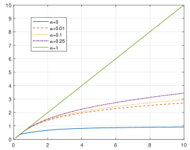
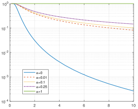
Figure 1: Given the activation function $\mathfrak{r}$ in (21) and $\alpha=(0,0.01,0.1,0.25,1)$; left plot: mappings $h$; right plot: moduli of strong monotonicity of mappings $H$ on $\{x:\|x\|_{\Sigma}\leq r\}$ as function of $r$.

3.2 Stochastic Mirror Descent algorithm

In this section, we describe the statistical properties of approximate solutions of Algorithm 1 when applied to the sparse recovery problem. We shall use the following distance-generating function of the $\ell_{1}$-ball of ${\mathbf{R}}^{n}$ (cf. [27, Section 5.7.1])

$$\theta(x)={c\over p}\|x\|_{p}^{p},\quad p=\left\{\begin{array}[]{ll}2,&n=2\\ 1+\frac{1}{\ln(n)},&n\geq 3,\end{array}\right.\quad c=\left\{\begin{array}[]{ll}2,&n=2,\\ e\ln n,&n\geq 3.\end{array}\right.$$ (26)

It immediately follows that $\theta$ is strongly convex with modulus 1 w.r.t. the norm $\|\cdot\|_{1}$ on its unit ball, and that $\Theta\leq e\ln n$. In particular, Theorem 2.1 entails the following statement.

Proposition 3.2

For $t\gtrsim\sqrt{\ln N}$, assuming the samples budget is large enough, i.e., $N\geq m_{0}$ (so that at least one stage of the preliminary phase of Algorithm 1 is completed), the approximate solution $\widehat{x}_{N}$ output satisfies with probability at least $1-Ce^{-t}\ln N$,

$${\|\widehat{x}_{N}-x_{*}\|_{1}}\lesssim R\exp\left\{-c\frac{{\underline{r}}\kappa_{\Sigma}}{{\overline{r}}{\overline{\nu}}^{2}}{N\over s({\ln n}+t)}\right\}+\frac{\sigma{\overline{\nu}}s}{{\underline{r}}\kappa_{\Sigma}}\sqrt{\frac{{\ln n}+t}{N}}$$ (27)

The corresponding solution $\widehat{x}^{(b)}_{N}$ of the minibatch variant of the algorithm satisfies with probability $\geq 1-Ce^{-t}\ln N$,

$${\|\widehat{x}_{N}^{(b)}-x_{*}\|_{1}}\lesssim R\exp\left\{-c\frac{{\underline{r}}\kappa_{\Sigma}}{{\overline{r}}{\overline{\nu}}^{2}}{N\over s\left({\ln n}+t\right)}\right\}+\frac{\sigma{\overline{\nu}}s}{{\underline{r}}\kappa_{\Sigma}}\sqrt{\frac{{\ln n}\left({\ln n}+t\right)}{N}}$$

Remark 3.2

Bounds for the $\ell_{1}$-norm of the error ${\widehat{x}}_{N}-x_{*}$ (or $\widehat{x}_{N}^{(b)}-x_{*}$) established in Proposition 3.2 allows us to quantify prediction error $g({\widehat{x}}_{N})-g(x_{*})$ (and $g({\widehat{x}}^{(b})_{N})-g(x_{*})$, and also lead to bounds for $\|{\widehat{x}}_{N}-x_{*}\|_{\Sigma}$ and $\|{\widehat{x}}_{N}-x_{*}\|_{2}$ (respectively, for $\|{\widehat{x}}_{N}^{(b)}-x_{*}\|_{\Sigma}$ and $\|{\widehat{x}}_{N}^{(b)}-x_{*}\|_{2}$). For instance, Proposition 2.1 in the present setting implies the bound on the prediction error after $N$ steps of the algorithm that reads

$$g({\widehat{x}}_{N})-g(x_{*})\lesssim{R^{2}\kappa_{\Sigma}{\underline{r}}\over s}\exp\left\{-\frac{c\kappa_{\Sigma}{\underline{r}}}{\delta^{2}{\overline{r}}{\overline{\nu}}^{2}}{N\over s(\Theta+t)}\right\}+{\sigma^{2}{\overline{\nu}}^{2}s(\Theta+t)\over\kappa_{\Sigma}{\underline{r}}N}$$

with probability $\geq 1-C\ln Ne^{-t}$. We conclude by (16) that

$$\|{\widehat{x}}_{N}-x_{*}\|_{2}^{2}\leq\kappa_{\Sigma}^{-1}\|{\widehat{x}}_{N}-x_{*}\|^{2}_{\Sigma}\leq 2\kappa_{\Sigma}^{-1}{\underline{r}}^{-1}[g({\widehat{x}}_{N})-g(x_{*})]$$

$$\quad\lesssim{R^{2}\over s}\exp\left\{-\frac{c\kappa_{\Sigma}{\underline{r}}}{\delta^{2}{\overline{r}}{\overline{\nu}}^{2}}{N\over s(\Theta+t)}\right\}+{\sigma^{2}{\overline{\nu}}^{2}s(\Theta+t)\over\kappa^{2}_{\Sigma}{\underline{r}}^{2}N}.$$

In other words, the error $\|{\widehat{x}}_{N}-x_{*}\|_{2}$ converges geometrically to the “asymptotic rate” ${\sigma{\overline{\nu}}\over\kappa_{\Sigma}{\underline{r}}}\sqrt{s(\Theta+t)\over N}$ which is the “standard” rate established in the setting (cf. [1, 5, 35], etc).

Remark 3.3

The proposed approach allows also to address the situation in which regressors are not a.s. bounded. For instance, consider the case of random regressors with i.i.d sub-Gaussian entries such that

$$\forall j\leq n,\quad{\mathbf{E}}\left[\exp\left(\tfrac{[\phi_{i}]_{j}^{2}}{\varkappa^{2}}\right)\right]\leq 1.$$

Using the fact that the maximum of uniform norms $\|\phi_{i}\|_{\infty}$, $1\leq i\leq m$, concentrates around $\varkappa\sqrt{\ln mn}$ along with independence of noises $\xi_{i}$ of $\phi_{i}$, the “smoothness” and “sub-Gaussianity” assumptions of Proposition 3.2 can be stated “conditionally” to the event $\left\{\omega:\;\max_{i\leq m}\|\phi_{i}\|_{\infty}^{2}\lesssim\varkappa^{2}(\ln[mn]+t)\right\}$ of probability greater than $1-e^{-t}$. For instance, when replacing the bound for the uniform norm of regressors with $\varkappa^{2}(\ln[mn]+t)$ in the definition of algorithm parameters and combining with appropriate deviation inequality for martingales (cf., e.g., [4]), one arrives at the bound for the error $\|\widehat{x}_{N}-x_{*}\|_{1}$ of Algorithm 1 which is similar to (27) of Proposition 3.2 in which ${\overline{\nu}}$ is replaced with $\varkappa\sqrt{\ln[mn]+t}$.

3.3 Numerical experiments

In this section, we present results of a small simulation study illustrating the theoretical part of the previous section. We consider the GLR model (15) with activation function (21) where $\alpha=1/2$. In our simulations, $x_{*}$ is an $s$-sparse vector with $s$ nonvanishing components sampled independently from the standard $s$-dimensional Gaussian distribution; regressors $\phi_{i}$ are sampled from a multivariate Gaussian distribution $\phi\sim\mathcal{N}(0,\Sigma)$, where $\Sigma$ is a diagonal covariance matrix with diagonal entries $\sigma_{1}\leq...\leq\sigma_{n}$. In Figure 2 we report on the experiment in which we compare the performance of the CSMD-SR algorithm from Section 2.3 to that of four other methods. The contenders are (1) “vanilla” non-Euclidean SMD algorithm constrained to the $\ell_{1}$-ball equipped with the distance generating function (26), (2) composite non-Euclidean dual averaging algorithm ($p$-Norm RDA) from [47], (3) multistage SMD-SR of [23], and (4) “vanilla” Euclidean SGD. The regularization parameter of the $\ell_{1}$ penalty in (2) is set to the theoretically optimal value $\lambda=2\sigma\sqrt{2\log(n)/T}$. The corresponding dimension of the parameter space is $n=500000$, the sparsity level of the optimal point $x_{*}$ is $s=200$, and the “total budget” of oracle calls is $N=250000$; we use the identity regressor covariance matrix ($\Sigma=I_{n}$) and $\sigma\in\{0.001,0.1\}$. To reduce computation time we use the minibatch versions of the multi-stage algorithms—CSMD-SR and algorithm (3)), the data to compute stochastic gradient realizations $\nabla G(x_{i},\omega)=\phi(\mathfrak{r}(\phi^{T}x_{i})-\eta)$ at the current search point $x_{i}$ being generated “on the fly.” We repeat simulations 20 times and plot the median value along with the first and the last deciles of the error $\|{\widehat{x}}_{i}-x_{*}\|_{1}$ at each iteration of the algorithm against the number of oracle calls.

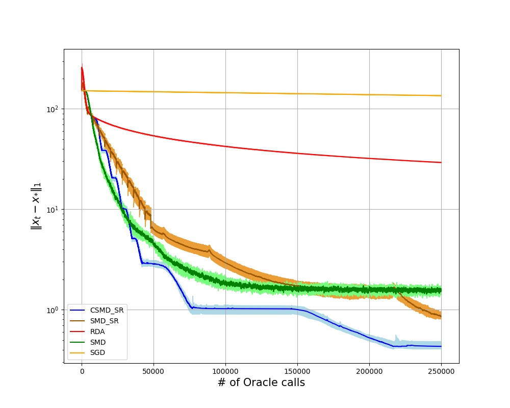
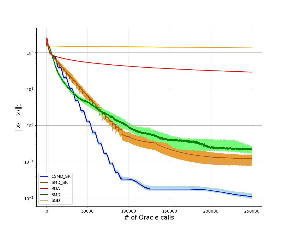
$\sigma=0.1$	$\sigma=0.001$

Figure 2: CSMD-SR and “vanilla” SMD in Generalized Linear Regression problem: $\ell_{1}$ error as a function of the number of oracle calls

The proposed method outperforms other algorithms which struggle to reach the regime where the stochastic noise is dominant.

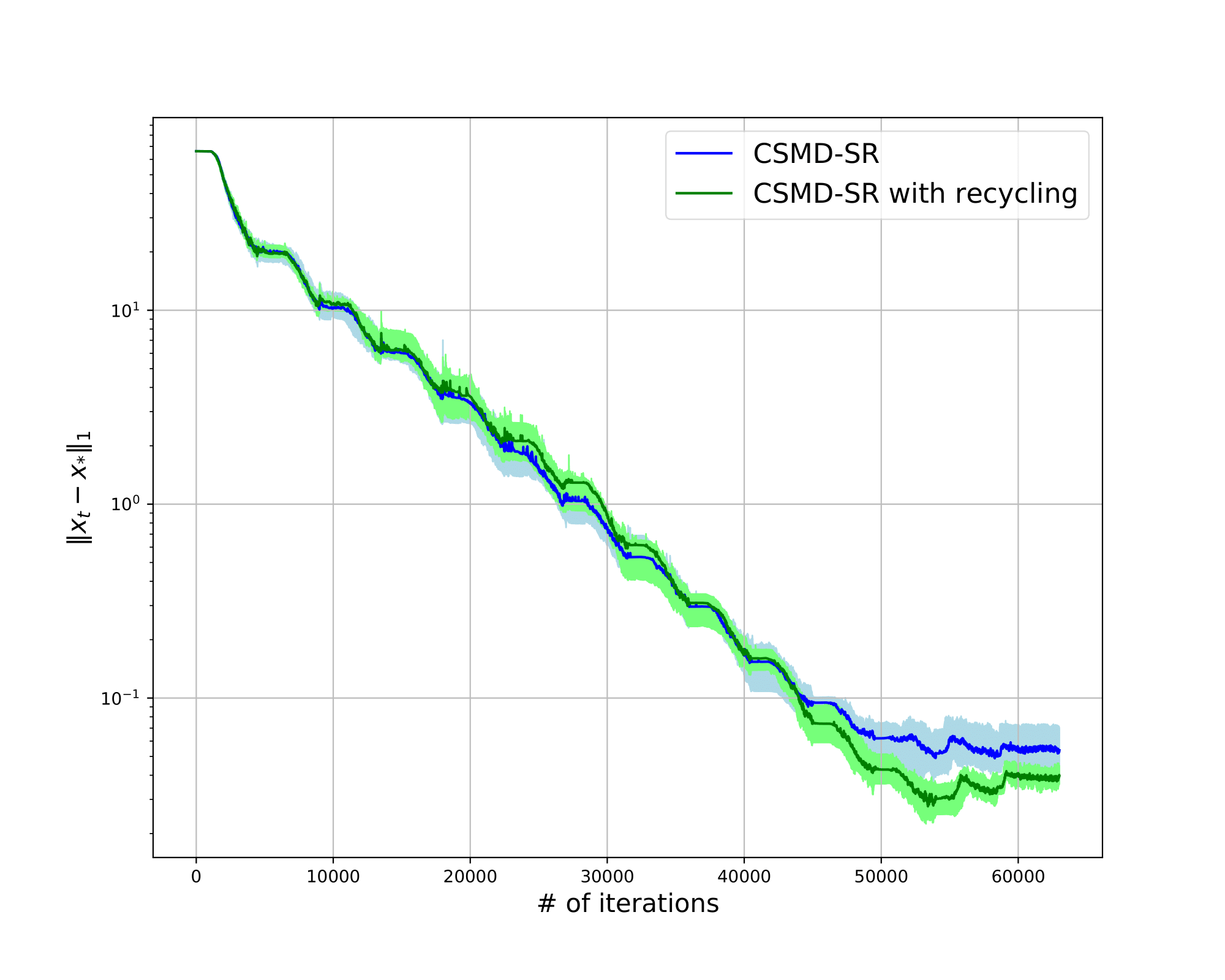
Figure 3: Preliminary stages of the CSMD-SR and its variant with data recycling: linear regression experiment (left pane), GLR with activation $\mathfrak{r}_{1/10}(t)$ (right pane).

In the second experiment we report on here, we study the behavior of the multistage algorithm derived from Algorithm 2 in which, instead of using independent data samples, we reuse the same data at each stage of the method. In Figure 3 we present results of comparison of the CSMD-SR algorithm with its variant with data recycle. This version is of interest as it attains fast the noise regime while using limited amount of samples. In our first experiment, we consider linear regression problem with parameter dimension $n=100\,000$ and sparsity level $s=75$ of the optimal solution; we consider the GLR model (15) with activation function $\mathfrak{r}_{1/10}(t)$ in the second experiment. We choose $\Sigma=I_{n}$ and $\sigma=0.001$; we run 14 (preliminary) stages of the algorithm with $m_{0}=3500$ in the first simulation and $m_{0}=4500$ in the second. We believe that the results speak for themselves.

Acknowledgements

This work was supported by Multidisciplinary Institute in Artificial intelligence MIAI @ Grenoble Alpes (ANR-19-P3IA-0003), “Investissements d’avenir” program (ANR20-CE23-0007-01), FAIRPLAY project, LabEx Ecodec (ANR11-LABX-0047), and ANR-19-CE23-0026. The authors would also like to acknowledge CRITEO AI Lab for supporting this work.

Appendix A Proofs

We use notation ${\mathbf{E}}_{i}$ for conditional expectation given $x_{0}$ and $\omega_{1},...,\omega_{i}$.

A.1 Proof of Proposition 2.1

The result of Proposition 2.1 is an immediate consequence of the following statement.

Proposition A.1

Let

$$f(x)=\mbox{\small$\frac{1}{2}$}g(x)+h(x),\quad x\in X.$$

In the situation of Section 2.2, let $\gamma_{i}\leq(4\nu)^{-1}$ for all $i=0,1,...$, and let $\widehat{x}_{m}$ be defined in (10), where $x_{i}$ are iterations (9). Then for any $t\geq 2\sqrt{2+\ln m}$ there is $\overline{\Omega}_{m}\subset\Omega$ such that $\hbox{\rm Prob}(\overline{\Omega}_{m})\geq 1-4e^{-t}$ and for all $\omega^{m}=[\omega_{1},...,\omega_{m}]\in\overline{\Omega}_{m}$,

$$\left(\sum_{i=0}^{m-1}\gamma_{i}\right)[f(\widehat{x}_{m})-f(x_{*})] \leq\sum_{i=0}^{m-1}\Big{[}\mbox{\small$\frac{1}{2}$}\gamma_{i}{\langle}\nabla g(x_{i}),x_{i}-x_{*}{\rangle}+\gamma_{i+1}(h(x_{i+1})-h(x_{*}))\Big{]}$$

$$\leq V({x_{0}},x_{*})+\gamma_{0}[h(x_{0})-h(x_{*})]-\gamma_{m}[h(x_{m})-h(x_{*})]$$

$$\qquad+V(x_{0},x_{*})+{15}tR^{2}+\sigma^{2}_{*}\left[{7}\sum_{i=0}^{m-1}\gamma_{i}^{2}+24t\overline{\gamma}^{2}\right].$$ (28)

In particular, when using the constant stepsize strategy with $\gamma_{i}\equiv\gamma$, $0<\gamma\leq(4\nu)^{-1}$, one has

$$\mbox{\small$\frac{1}{2}$}[g({\widehat{x}}_{m})-g(x_{*})]+[h({\widehat{x}}_{m})-h(x_{*})]$$

$$\qquad\leq{V(x_{0},x_{*})+{15}tR^{2}\over\gamma m}+{h(x_{0})-h(x_{m})\over m}+\gamma\sigma^{2}_{*}\left({7}+{24t\over m}\right).$$ (29)

Proof.

Denote $H_{i}=\nabla G(x_{i-1},\omega_{i})$. In the sequel, we use the shortcut notation $\vartheta(z)$ and $V(x,z)$ for $\vartheta_{x_{0}}^{R}(z)$ and $V_{x_{0}}(x,z)$ when exact values $x_{0}$ and $R$ are clear from the context.

1^o.

From the definition of $x_{i}$ and of the composite prox-mapping (8) (cf. Lemma A.1 of [40]), we conclude that there is $\eta_{i}\in\partial h(x_{i})$ such that

$${\langle}\gamma_{i-1}H_{i}+\gamma_{i}\eta_{i}+\nabla\vartheta(x_{i})-\nabla\vartheta(x_{i-1}),z-x_{i}{\rangle}\geq 0,\;\;\forall\;z\in{\cal X},$$

implying, as usual [12], that $\forall z\in{\cal X}$

$${\langle}\gamma_{i-1}H_{i}+\gamma_{i}\eta_{i},x_{i}-z{\rangle}\leq V(x_{i-1},z)-V(x_{i},z)-V(x_{i-1},x_{i}).$$

In particular,

$$\gamma_{i-1}{\langle}H_{i},x_{i-1}-x_{*}{\rangle}+\gamma_{i}{\langle}\eta_{i},x_{i}-x_{*}{\rangle}$$

$$\leq V(x_{i-1},x_{*})-V(x_{i},x_{*})-V(x_{i-1},x_{i})+\gamma_{i-1}{\langle}H_{i},x_{i-1}-x_{i}{\rangle}$$

$$\leq V(x_{i-1},x_{*})-V(x_{i},x_{*})+\mbox{\small$\frac{1}{2}$}\gamma^{2}_{i-1}\|H_{i}\|_{*}^{2}.$$

Observe that due to the Lipschitz continuity of $\nabla G(\cdot,\omega)$ one has

$$\nu{\langle}\nabla G(x,\omega)-\nabla G(x^{\prime},\omega),x-x^{\prime}{\rangle}\geq\|\nabla G(x,\omega)-\nabla G(x^{\prime},\omega)\|_{*}^{2},\quad\forall x,x^{\prime}\in{\cal X},$$ (30)

so that

$$\|\nabla G(x,\omega)\|_{*}^{2} \leq 2\|\nabla G(x,\omega)-\nabla G(x_{*},\omega)\|_{*}^{2}+2\|\nabla G(x_{*},\omega)\|_{*}^{2}$$

$$\leq 2\nu{\langle}\nabla G(x,\omega)-\nabla G(x_{*},\omega),x-x_{*}{\rangle}+2\|\nabla G(x_{*},\omega)\|_{*}^{2}$$

$$=2\nu{\langle}\nabla G(x,\omega),x-x_{*}{\rangle}-2\nu{\langle}\nabla G(x_{*},\omega),x-x_{*}{\rangle}+2\|\nabla G(x_{*},\omega)\|_{*}^{2}$$

so that

$$\gamma_{i-1}{\langle}H_{i},x_{i-1}-x_{*}{\rangle}+\gamma_{i}{\langle}\eta_{i},,x_{i}-x_{*}{\rangle}$$

$$\leq V(x_{i-1},x_{*})-V(x_{i},x_{*})+\gamma^{2}_{i-1}[\nu{\langle}H_{i},x_{i-1}-x_{*}{\rangle}-\nu\zeta_{i}+\tau_{i}]$$

where $\zeta_{i}={\langle}\nabla G(x_{*},\omega_{i}),x_{i-1}-x_{*}{\rangle}$ and $\tau_{i}=\|\nabla G(x_{*},\omega)\|_{*}^{2}$. As a result, by convexity of $h$ we have for $\gamma_{i}\leq(4\nu)^{-1}$

$$\mbox{\small$\frac{3}{4}$}\gamma_{i-1}{\langle}\nabla g(x_{i-1}),x_{i-1}-x_{*}{\rangle}+\gamma_{i}[h(x_{i})-h(x_{*})]$$

$$\leq(\gamma_{i-1}-\gamma_{i-1}^{2}\nu){\langle}\nabla g(x_{i-1}),x_{i-1}-x_{*}{\rangle}+\gamma_{i}{\langle}\eta_{i},x_{i}-x_{*}{\rangle}$$

$$\leq V(x_{i-1},x_{*})-V(x_{i},x_{*})+(\gamma_{i-1}-\gamma_{i-1}^{2}\nu){\langle}\xi_{i},x_{i-1}-x_{*}{\rangle}+\gamma_{i-1}^{2}[\tau_{i}-\nu\zeta_{i}]$$

where we put $\xi_{i}=H_{i}-\nabla g(x_{i-1})$. When summing from $i=1$ to $m$ we obtain

$$\sum_{i=1}^{m}\gamma_{i-1}\Big{(}\mbox{\small$\frac{3}{4}$}{\langle}\nabla g(x_{i-1}),x_{i-1}-x_{*}{\rangle}+[h(x_{i-1})-h(x_{*})]\Big{)}$$

$$\qquad\leq V(x_{0},x_{*})+\underbrace{\sum_{i=1}^{m}[\gamma_{i-1}^{2}(\tau_{i}-\nu\zeta_{i})+\gamma_{i-1}(1-\gamma_{i-1}\nu){\langle}\xi_{i},x_{i-1}-x_{*}{\rangle}]}_{=:R_{m}}$$

$$\qquad\qquad+\gamma_{0}[h(x_{0})-h(x_{*})]-\gamma_{m}[h(x_{m})-h(x_{*})].$$ (31)

2^o.

We have

$$\gamma_{i-1}{\langle}\xi_{i},x_{i-1}-x_{*}{\rangle} = \gamma_{i-1}\overbrace{{\langle}[\nabla G(x_{i-1},\omega_{i})-\nabla G(x_{*},\omega_{i})]-\nabla g(x_{i-1}),x_{i-1}-x_{*}{\rangle}}^{\upsilon_{i}}$$

$$+\gamma_{i-1}{\langle}\nabla G(x_{*},\omega_{i}),x_{i-1}-x_{*}{\rangle}$$

$$= \gamma_{i-1}[\upsilon_{i}+\zeta_{i}],$$

so that

$$R_{m}={\sum_{i=1}^{m}\gamma_{i-1}^{2}\tau_{i}}+{\sum_{i=1}^{m}(\gamma_{i-1}-\gamma^{2}_{i-1}\nu)\upsilon_{i}}+{\sum_{i=1}^{m}(\gamma_{i-1}-2\nu\gamma_{i-1}^{2})\zeta_{i}}=:r^{(1)}_{m}+r^{(2)}_{m}+r^{(3)}_{m}.$$ (32)

Note that $r^{(3)}_{m}$ is a sub-Gaussian martingale. Indeed, one has ${\mathbf{E}}_{i-1}\{\zeta_{i}\}=0$ a.s., and

$$|\zeta_{i}|\leq\|x_{i-1}-x_{*}\|\,\|\nabla G(x_{*},\omega)\|_{*},$$

so that by the sub-Gaussian hypothesis (6), ${\mathbf{E}}_{i-1}\Big{\{}\exp\Big{(}\underbrace{\zeta^{2}_{i}\over 4R^{2}\sigma_{*}^{2}}_{\nu_{*}^{2}}\Big{)}\Big{\}}\leq\exp(1)$. As a result (cf. the proof of Proposition 4.2 in [28]),

$$\forall t\quad{\mathbf{E}}_{i-1}\left\{e^{t\zeta_{i}}\right\}\leq\exp\left(t{\mathbf{E}}_{i-1}\{\zeta_{i}\}+{\tfrac{3}{4}t^{2}\nu^{2}_{*}}\right)=\exp\left({3t^{2}R^{2}\sigma^{2}_{*}}\right),$$

and applying (37a) to $S_{m}=r_{m}^{(3)}$ with

$$r_{m}=6R^{2}\sigma_{*}^{2}\sum_{i=0}^{m-1}(\gamma_{i}-2\nu\gamma_{i}^{2})^{2}\leq{6}R^{2}\sigma_{*}^{2}\sum_{i=0}^{m-1}\gamma^{2}_{i}$$

we conclude that for some $\Omega^{(3)}_{m}$ such that $\hbox{\rm Prob}(\Omega^{(3)}_{m})\geq 1-e^{-t}$ and all $\omega^{m}\in\Omega^{(3)}_{m}$

$$r^{(3)}_{m}\leq 2\sqrt{{3tR^{2}\sigma_{*}^{2}}\sum_{i=0}^{m-1}\gamma_{i}^{2}}\leq{{3}tR^{2}}+{3}\sigma_{*}^{2}\sum_{i=0}^{m-1}\gamma_{i}^{2}.$$ (33)

Next, again by (6), due to the Jensen inequality, ${\mathbf{E}}_{i-1}\{\tau_{i}\}\leq\sigma_{*}^{2}$, and

$${\mathbf{E}}_{i-1}\left\{\exp\left(t\|\nabla G(x_{*},\omega_{i})\|_{*}\right)\right\}\leq\exp\left(t{\mathbf{E}}_{i-1}\{\|\nabla G(x_{*},\omega_{i})\|_{*}\}+{\tfrac{3}{4}t^{2}\sigma^{2}_{*}}\right)\leq\exp\left(t\sigma_{*}+\tfrac{3}{4}t^{2}\sigma^{2}_{*}\right).$$

Thus, when setting

$$\mu_{i}=\gamma_{i-1}\sigma_{*},\;\;s_{i}^{2}=\tfrac{3}{2}\gamma_{i-1}\sigma_{*}^{2},\;\;\overline{s}=\max_{i}\gamma_{i}s_{i},$$

$M_{m}=r^{(1)}_{m}$, $v_{m}+h_{m}=\tfrac{21}{4}\sigma_{*}^{4}\sum_{i=0}^{m-1}\gamma_{i}^{4}$, and applying the bound (37b) of Lemma A.1 we obtain

$$r^{(1)}_{m}\leq 3\sigma^{2}_{*}\sum_{i=0}^{m-1}\gamma_{i}^{2}+\underbrace{\sqrt{21t\sigma_{*}^{4}\sum_{i=0}^{m-1}\gamma_{i}^{4}}}_{=:\Delta^{(1)}_{m}}+3t\overline{\gamma}^{2}\sigma_{*}^{2}$$

for $\overline{\gamma}=\max_{i}\gamma_{i}$ and $\omega^{m}\in\Omega^{(1)}_{m}$ where $\Omega^{(1)}_{m}$ is of probability at least $1-e^{-x}$. Because

$$\overline{\gamma}^{2}\sum_{i=0}^{m-1}\gamma_{i}^{2}\geq\sum_{i=0}^{m-1}\gamma_{i}^{4},$$

whenever $\sqrt{21t\sigma_{*}^{4}\sum_{i=0}^{m-1}\gamma_{i}^{4}}\geq\sum_{i=0}^{m-1}\gamma_{i}^{2},$ one has $21t\overline{\gamma}^{2}\geq\sum_{i=0}^{m-1}\gamma_{i}^{2}$ and

$$21t\sum_{i=0}^{m-1}\gamma_{i}^{4}\leq{21t\overline{\gamma}^{2}\sum_{i=0}^{m-1}\gamma_{i}^{2}}\leq(21t\overline{\gamma}^{2})^{2}$$

Thus,

$$\Delta^{(1)}_{m}\leq\min\left[21t\sigma^{2}_{*}\overline{\gamma}^{2},\sigma_{*}^{2}\sum_{i=0}^{m-1}\gamma_{i}^{2}\right]\leq 21t\sigma^{2}_{*}\overline{\gamma}^{2}+\sigma_{*}^{2}\sum_{i=0}^{m-1}\gamma_{i}^{2},$$

and

$$r^{(1)}_{m}\leq\sigma^{2}_{*}\left[4\sum_{i=0}^{m-1}\gamma_{i}^{2}+24t\overline{\gamma}^{2}\right]$$ (34)

for $\omega^{m}\in\Omega^{(1)}_{m}$.

Finally, by the Lipschitz continuity of $\nabla G$ (cf. (30)), when taking expectation w.r.t. the distribution of $\omega_{i}$, we get

$${\mathbf{E}}_{i-1}\{\upsilon_{i}^{2}\} \leq 4R^{2}{\mathbf{E}}_{i-1}\{\|\nabla G(x_{i-1},\omega_{i})-\nabla G(x_{*},\omega_{i})\|_{*}^{2}\}$$

$$\leq 4R^{2}\nu{\mathbf{E}}_{i-1}\{{\langle}\nabla G(x_{i-1},\omega_{i})-\nabla G(x_{*},\omega_{i}),x_{i-1}-x_{*}{\rangle}\}=4R^{2}\nu{\langle}\nabla g(x_{i-1}),x_{i-1}-x_{*}{\rangle}.$$

On the other hand, one also has $|\upsilon_{i}|\leq 2\nu\|x_{i-1}-x_{i}\|^{2}\leq 8\nu R^{2}$. We can now apply Lemma A.2 with $\sigma_{i}^{2}=4\gamma_{i-1}^{2}R^{2}\nu{\langle}\nabla g(x_{i-1}),x_{i-1}-x_{*}{\rangle}$ to conclude that for $t\geq 2\sqrt{2+\ln m}$

$$r_{m}^{(2)}\leq{4}\underbrace{\sqrt{tR^{2}\nu\sum_{i=0}^{m-1}\gamma_{i}^{2}{\langle}\nabla g(x_{i}),x_{i}-x_{*}{\rangle}}}_{=:\Delta^{(2)}_{m}}+{{16}t\nu R^{2}\overline{\gamma}}$$

for all $\omega^{m}\in\Omega^{(2)}_{m}$ such that $\hbox{\rm Prob}(\Omega^{(2)}_{m})\geq 1-2e^{-t}$. Note that

$$\Delta_{m}^{(2)}\leq{2}{tR^{2}}+{\tfrac{1}{4}}\nu\sum_{i=0}^{m-1}\gamma_{i}^{2}{\langle}\nabla g(x_{i}),x_{i}-x_{*}{\rangle},$$

and $\gamma_{i}\leq(4\nu)^{-1}$, so that

$$r_{m}^{(2)}\leq\nu\sum_{i=0}^{m-1}\gamma_{i}^{2}{\langle}\nabla g(x_{i}),x_{i}-x_{*}{\rangle}+{12}{tR^{2}}\leq\tfrac{1}{4}\sum_{i=0}^{m-1}\gamma_{i}{\langle}\nabla g(x_{i}),x_{i}-x_{*}{\rangle}+{12}{tR^{2}}$$ (35)

for $\omega^{m}\in\Omega^{(2)}_{m}$.

3^o.

When substituting bounds (33)–(35) into (32) we obtain

$$R_{m} \leq \tfrac{1}{4}\sum_{i=0}^{m-1}\gamma_{i}{\langle}\nabla g(x_{i}),x_{i}-x_{*}{\rangle}+{12}{tR^{2}}+\sigma^{2}_{*}\left[4\sum_{i=0}^{m-1}\gamma_{i}^{2}+24t\overline{\gamma}^{2}\right]+{2}\sqrt{{3}tR^{2}\sigma_{*}^{2}\sum_{i=0}^{m-1}\gamma_{i}^{2}}$$

$$\leq \tfrac{1}{4}\sum_{i=0}^{m-1}\gamma_{i}{\langle}\nabla g(x_{i}),x_{i}-x_{*}{\rangle}+{15}tR^{2}+\sigma^{2}_{*}\left[{7}\sum_{i=0}^{m-1}\gamma_{i}^{2}+24t\overline{\gamma}^{2}\right]$$

for all $\omega^{m}\in\overline{\Omega}_{m}=\bigcap_{i=1}^{3}\Omega^{(i)}_{m}$ with $\hbox{\rm Prob}(\overline{\Omega}_{m})\geq 1-4e^{-t}$ and $t\geq 2\sqrt{2+\ln m}$.

When substituting the latter bound into (31) and utilizing the convexity of $g$ and $h$ we arrive at

$$\left(\sum_{i=0}^{m-1}\gamma_{i}\right)\Big{(}\mbox{\small$\frac{1}{2}$}[g({\widehat{x}}_{m})-g(x_{*})]+[h({\widehat{x}}_{m})-h(x_{*})]\Big{)}\leq\sum_{i=0}^{m-1}\gamma_{i}\Big{(}\mbox{\small$\frac{1}{2}$}[g(x_{i})-g(x_{*})]+[h(x_{i})-h(x_{*})]\Big{)}$$

$$\leq\sum_{i=1}^{m}\gamma_{i-1}\Big{(}\mbox{\small$\frac{1}{2}$}{\langle}\nabla g(x_{i-1},x_{i-1}-x_{*}{\rangle}+[h(x_{i-1})-h(x_{*})]\Big{)}$$

$$\leq V(x_{0},x_{*})+{15}tR^{2}+\sigma^{2}_{*}\left[{7}\sum_{i=0}^{m-1}\gamma_{i}^{2}+24t\overline{\gamma}^{2}\right]+\gamma_{0}[h(x_{0})-h(x_{*})]-\gamma_{m}[h(x_{m})-h(x_{*})].$$

In particular, for constant stepsizes $\gamma_{i}\equiv\gamma$ we get

$$\mbox{\small$\frac{1}{2}$}[g({\widehat{x}}_{m})-g(x_{*})]+[h({\widehat{x}}_{m})-h(x_{*})]$$

$$\quad\leq{V(x_{0},x_{*})+{15}tR^{2}\over\gamma m}+{h(x_{0})-h(x_{m})\over m}+\gamma\sigma^{2}_{*}\left({7}+\frac{24t}{m}\right).$$

This implies the first statement of the proposition.

5^o.

To prove the bound for the minibatch solution ${\widehat{x}}_{m}^{(L)}=\left(\sum_{i=0}^{m-1}\gamma_{i}\right)^{-1}\sum_{i=0}^{m-1}\gamma_{i}x_{i}^{(L)}$, it suffices to note that minibatch gradient observation $H(x,\omega^{(L)})$ is Lipschitz-continuous with Lipschitz constant $\nu$, and that $H(x_{*},\omega^{(L)})$ is sub-Gaussian with parameter $\sigma_{*}^{2}$ replaced with ${\overline{\sigma}}^{2}_{*,L}\lesssim{\Theta\sigma_{*}^{2}\over L}$, see Lemma A.3. $\Box$

A.2 Deviation inequalities

Let us assume that $(\xi_{i},{\cal F}_{i})_{i=1,2,...}$ is a sequence of sub-Gaussian random variables satisfying

$${\mathbf{E}}_{i-1}\left\{e^{t\xi_{i}}\right\}\leq e^{t\mu_{i}+\frac{t^{2}s_{i}^{2}}{2}},\hskip 14.22636pta.s.$$ (36)

for some nonrandom $\mu_{i},s_{i}$, $s_{i}\leq\overline{s}$. We denote by $S_{n}=\sum_{i=1}^{n}{\xi_{i}-\mu_{i}}$, $r_{n}=\sum_{i=1}^{n}{s_{i}^{2}}$, $v_{n}=\sum_{i=1}^{n}{s_{i}^{4}},M_{n}=\sum_{i=1}^{n}\xi_{i}^{2}-(s_{i}^{2}+\mu_{i}^{2})$, and $h_{n}=\sum_{i=1}^{n}2\mu_{i}^{2}s_{i}^{2}.$ The following well known result is provided for reader’s convenience.

Lemma A.1

For all $x>0$ one has

$$\hbox{\rm Prob}\left\{S_{n}\geq\sqrt{2xr_{n}}\right\} \leq e^{-x},$$ (37a)

$$\hbox{\rm Prob}\left\{M_{n}\geq 2\sqrt{x(v_{n}+h_{n})}+2x{\overline{s}}^{2}\right\} \leq e^{-x}.$$ (37b)

Proof.

The inequality (37a) is straightforward. To prove (37b), note that for $t<\frac{1}{2}\overline{s}^{-2}$ and $\eta\sim\mathcal{N}(0,1)$ independent of $\xi_{0},...,\xi_{n}$ , we have:

$${\mathbf{E}}_{i-1}\left\{e^{t\xi_{i}^{2}}\right\} ={\mathbf{E}}_{i-1}\left\{{\mathbf{E}}_{\eta}\left\{e^{\sqrt{2t}\xi_{i}\eta}\right\}\right\}={\mathbf{E}}_{\eta}\left\{{\mathbf{E}}_{i-1}\left\{e^{\sqrt{2t}\xi_{i}\eta}\right\}\right\}$$

$$\leq{\mathbf{E}}_{\eta}\left\{\exp\left\{\sqrt{2t}\eta\mu_{i}+t\eta^{2}s_{i}^{2}\right\}\right\}=(1-2ts_{i}^{2})^{-1/2}\exp\left\{\frac{t\mu_{i}^{2}}{1-2ts_{i}^{2}}\right\}\hskip 5.69046pt\text{a.s.},$$

and because, cf [31, Lemma 1],

$$-\tfrac{1}{2}\text{ln}(1-2ts_{i}^{2})+\frac{t\mu_{i}^{2}}{1-2ts_{i}^{2}}-t(s_{i}^{2}+\mu_{i}^{2})\leq\frac{t^{2}s_{i}^{2}(s_{i}^{2}+2\mu_{i}^{2})}{1-2ts_{i}^{2}}\leq\frac{t^{2}s_{i}^{2}(s_{i}^{2}+2\mu_{i}^{2})}{1-2t\overline{s}^{2}},$$

one has for $t<\tfrac{1}{2}\overline{s}^{-2}$

$${\mathbf{E}}\left\{e^{tM_{n}}\right\}\leq\exp\left\{\frac{t^{2}(v_{n}+h_{n})}{1-2t\overline{s}^{2}}\right\}.$$

By Lemma 8 of [6], this implies that

$$\hbox{\rm Prob}\left\{M_{n}\geq 2\sqrt{x(v_{n}+h_{n})}+2x{\overline{s}}^{2}\right\}\leq e^{-x}$$

for all $x>0$. $\Box$

Now, suppose that $\zeta_{i},\;i=1,2,...$ is a sequence of random variables satisfying

$${\mathbf{E}}_{i-1}\{\zeta_{i}\}=\mu_{i},\,{\mathbf{E}}_{i-1}\{\zeta_{i}^{2}\}\leq\sigma_{i}^{2},\;\;|\zeta_{i}|\leq 1\;\;\mathrm{a.s.}$$ (38)

Denote $M_{n}=\sum_{i=1}^{n}[\zeta_{i}-\mu_{i}]$ and $q_{n}=\sum_{i=1}^{n}\sigma_{i}^{2}$. Note that $q_{n}\leq n$.

Lemma A.2

Let $x\geq 1$; one has

$$\hbox{\rm Prob}\left\{M_{n}\geq\sqrt{2xq_{n}}+{x}\right\}\leq\left[e\left(2x\ln\left[{9n\over 2x}\right]+1\right)+1\right]e^{-x}.$$

In particular, for $x\geq 4\sqrt{2+\ln n}$ one has

$$\hbox{\rm Prob}\left\{M_{n}\geq\sqrt{2xq_{n}}+{x}\right\}\leq 2e^{-x/2}.$$

Proof. In the premise of the lemma, applying Bernstein’s inequality for martingales [4, 15] we obtain for all $x>0$ and $u>0$,

$$\hbox{\rm Prob}\left\{M_{n}\geq\sqrt{2xu}+{x\over 3},\,q_{n}\leq u\right\}\leq e^{-x}.$$

We conclude that

$$\hbox{\rm Prob}\left\{M_{n}\geq{x},\,q_{n}\leq{2x\over 9}\right\}\leq e^{-x},$$

and for any $u>0$

$$\hbox{\rm Prob}\left\{M_{n}\geq\sqrt{2(x+1)q_{n}}+{x\over 3},\,u\leq q_{n}\leq u\big{(}1+{1/x}\big{)}\right\}\leq e^{-x},$$

so that

$$\delta_{n}(x;u):=\hbox{\rm Prob}\left\{M_{n}\geq\sqrt{2xq_{n}}+{x\over 3},\,u\leq q_{n}\leq u\big{(}1+{1/x}\big{)}\right\}\leq e^{-x+1}.$$

Let now $u_{0}=2x/9$, $u_{j}=\min\{n,(1+1/x)^{j}u_{0}\}$, $j=0,...,J$, with

$$J=\left\rfloor\ln\big{[}{n/u_{0}}\big{]}\ln^{-1}[1+1/x]\right\lfloor.$$

Note that $\ln[1+1/x]\geq 1/(2x)$ for $x\geq 1$, so that

$$J\leq\ln\big{[}{n/u_{0}}\big{]}\ln^{-1}[1+1/x]+1\leq 2x\ln\big{[}{n/u_{0}}\big{]}+1.$$

On the other hand,

$$\hbox{\rm Prob}\left\{M_{n}\geq\sqrt{2xq_{n}}+{x}\right\} \leq e^{-x}+\sum_{j=1}^{J}\delta_{n}(x;u_{j})\leq e^{-x}+Je^{-x+1}$$

$$\leq \Big{[}e\Big{(}2x\ln\Big{[}{9n\over 2x}\Big{]}+1\Big{)}+1\Big{]}e^{-x}$$

Finally, we verify explicitly that for $x\geq 4\sqrt{2+\ln n}$ one has

$$\Big{[}e\Big{(}2x\ln\Big{[}{9n\over 2x}\Big{]}+1\Big{)}+1\Big{]}e^{-x/2}\leq 2,$$

implying that for such $x$

$$\hbox{\rm Prob}\left\{M_{n}\geq\sqrt{2xq_{n}}+{x}\right\}\leq 2e^{-x/2}. \Box$$

Let $(\xi_{i})_{i=1,...}$ be a sequence of independent random vectors in ${\mathbf{R}}^{n}$ such that

$${\mathbf{E}}_{i-1}\left\{\exp\left({\|\xi_{i}\|_{*}^{2}\over s^{2}}\right)\right\}\leq\exp(1),$$

and let $\eta=\sum_{i=1}^{m}\xi_{i}$, $m\in{\mathbf{Z}}_{+}$. We are interested in “sub-Gaussian characteristics” of r.v. $\zeta={\langle}u,\eta{\rangle}$ for some $u\in{\mathbf{R}}^{n}$, $\|u\|\leq R$, and of $\tau=\|\eta\|_{*}$.

Because ${\mathbf{E}}\{{\langle}u,\xi_{i}{\rangle}\}=0$ and $|{\langle}u,\xi_{i}{\rangle}|\leq\|u\|\,\|\xi_{i}\|_{*}$, for all $t$ one has (cf.,e.g., Proposition 4.2 of [28])

$${\mathbf{E}}\Big{\{}e^{t{\langle}u,\eta{\rangle}}\Big{\}}=\prod_{i=1}^{m}{\mathbf{E}}\Big{\{}e^{t{\langle}u,\xi_{i}{\rangle}}\Big{\}}\leq\prod_{i=1}^{m}\exp\left({\tfrac{3}{4}t^{2}s^{2}}\right)=\exp\left(\tfrac{3}{4}mt^{2}s^{2}\right).$$

Let $\xi_{\ell}$, $\ell=1,2,...$ be a sequence of independent random vectors $\xi_{\ell}\in E$, such that ${\mathbf{E}}\{\xi_{\ell}\}=0$ and ${\mathbf{E}}\Big{\{}e^{\|\xi_{\ell}\|_{*}^{2}/s^{2}}\Big{\}}\leq\exp(1)$. Denote $\eta_{j}=\sum_{\ell=1}^{j}\xi_{\ell}$. We have the following result.

Lemma A.3

$$\forall L\in{\mathbf{Z}}_{+}\quad{\mathbf{E}}\left\{\exp\left({\|\eta_{L}\|_{*}^{2}\over 10\Theta s^{2}L}\right)\right\}\leq\exp(1)$$ (39)

where $\Theta=\max_{\|z\|\leq 1}\theta(z)$ for the d.-g.f. $\theta$ of the unit ball of norm $\|\cdot\|$ in $E$, as defined in Section 2.2.

Proof. Let for $\eta\in E$, $\pi(\eta)=\sup_{\|z\|\leq 1}[{\langle}\eta,z{\rangle}-\theta(z)]$. Observe that for all $\beta>0$,

$$\|\eta_{L}\|_{*}=\sup_{\|z\|\leq 1}{\langle}\eta_{L},z{\rangle}\leq\max_{\|z\|\leq 1}\beta\theta(z)+\beta\pi(\eta_{L}/\beta)\leq\beta\Theta+\beta\pi\big{(}{\eta_{L}\over\beta}\big{)}.$$ (40)

On the other hand, we know (cf. [38, Lemma 1]) that $\pi$ is smooth with $\|\nabla\pi\|\leq 1$, and $\nabla\pi$ is Lipschitz-continuous w.r.t. to $\|\cdot\|_{*}$, i.e.,

$$\|\nabla\pi(z)-\nabla\pi(z^{\prime})\|\leq\|z-z^{\prime}\|_{*}\quad\forall z,z^{\prime}\in E.$$

As a consequence of Lipschitz continuity of $\pi$, when denoting $\pi_{\beta}(\eta)=\beta\pi\big{(}{\eta\over\beta}\big{)}$, we have

$$\pi_{\beta}(\eta_{j-1}+\xi_{j})-\pi_{\beta}(\eta_{j-1})\leq\|\xi_{j}\|_{*},$$

so that ${\mathbf{E}}\left\{\exp\left([\pi_{\beta}(\eta_{j})-\pi_{\beta}(\eta_{j-1})]^{2}/s^{2}\right)\right\}\leq\exp(1)$. Furthermore,

$$\pi_{\beta}(\eta_{j-1}+\xi_{j})\leq\pi_{\beta}(\eta_{j-1})+{\langle}\nabla\pi_{\beta}(\eta_{j-1}),\xi_{j}/\beta{\rangle}+{\|\xi_{j}\|_{*}^{2}/\beta},$$

and, because $\eta_{j-1}$ does not depend on $\xi_{j}$ and ${\mathbf{E}}\{\|\xi_{j}\|_{*}^{2}\}\leq s^{2}$, we get

$${\mathbf{E}}_{j-1}\{\pi_{\beta}(\eta_{j})-\pi_{\beta}(\eta_{j-1})\}\leq{s^{2}/\beta}.$$

By [28, Proposition 4.2] we conclude that random variables $\delta_{j}=\pi_{\beta}(\eta_{j})-\pi_{\beta}(\eta_{j-1})$ satisfy for all $t\geq 0$,

$${\mathbf{E}}_{j-1}\left\{e^{t\delta_{j}}\right\}\leq\exp\left(ts^{2}\beta^{-1}+{\tfrac{3}{4}t^{2}s^{2}}\right).$$

Consequently,

$${\mathbf{E}}\left\{e^{t\pi_{\beta}(\eta_{L})}\right\}\leq{\mathbf{E}}\left\{e^{t\pi_{\beta}(\eta_{L-1})}\right\}\exp\left({ts^{2}\beta^{-1}}+{\tfrac{3}{4}t^{2}s^{2}}\right)\leq\exp\left({ts^{2}L\beta^{-1}}+{\tfrac{3}{4}t^{2}s^{2}L}\right).$$

When substituting the latter bound into (40), we obtain for $\beta^{2}={s^{2}L/\Theta}$

$${\mathbf{E}}\left\{e^{t\|\eta_{L}\|_{*}}\right\}\leq\exp\left(ts\sqrt{\Theta L}+\tfrac{3}{4}t^{2}s^{2}L\right)\quad\forall t\geq 0.$$ (41)

To complete the proof of the lemma, it remains to show that (41) implies (39). This is straightforward. Indeed, for $\chi\sim{\cal N}(0,1),\,\alpha>0$ and $\zeta=\|\eta_{L}\|_{*}$ one has

$${\mathbf{E}}\Big{\{}e^{\alpha\zeta^{2}}\Big{\}} ={\mathbf{E}}\left\{{\mathbf{E}}_{\eta}\left(e^{\sqrt{2\alpha}\zeta\chi}\right)\right\}={\mathbf{E}}_{\chi}\left\{{\mathbf{E}}\left\{e^{\sqrt{2\alpha}\zeta\chi}\right\}\right\}$$

$$\leq{\mathbf{E}}_{\chi}\left\{\exp\left(\sqrt{2\alpha\Theta L}\,s\chi+\tfrac{3}{2}\alpha Ns^{2}\chi^{2}\right)\right\}=(1-3\alpha Ns^{2})^{-1/2}\exp\left\{\frac{\alpha\Theta Ls^{2}}{1-3\alpha Ns^{2}}\right\}$$

When setting $\alpha=(10\Theta s^{2}L)^{-1}$, we conclude that

$${\mathbf{E}}\Big{\{}e^{\alpha\zeta^{2}}\Big{\}}\leq\exp(1)$$

due to $\Theta\geq 1/2$. $\Box$

A.3 Proof of Theorem 2.1

We start with analysing the behaviour of the approximate solution ${\widehat{x}}^{k}_{m_{0}}$ at the stages of the preliminary phase of the procedure.

Lemma A.4

Let $m_{0}=\lceil 64\delta^{2}\rho\nu s(4\Theta+{60}t)\rceil$ ((here $\lceil a\rceil$ stands for the smallest integer greater or equal to $a$), $\gamma=(4\nu)^{-1}$, and let $t$ satisfy $t\geq 4\sqrt{2+\log(m_{0})}$.

Suppose that $R\geq 2\delta\sigma_{*}\sqrt{6\rho s/\nu}$, that initial condition $x_{0}$ of Algorithms 1 and 2 satisfies $\|x_{0}-x_{*}\|\leq R$, and that at the stage $k$ of the preliminary phase we choose

$$\kappa_{k}=R_{k-1}\sqrt{\frac{\nu(4\Theta+{60}t)}{\rho sm_{0}}}$$ (42)

where $(R_{k})_{k\geq 0}$ is defined recursively:

$$R_{k+1}=\mbox{\small$\frac{1}{2}$}{R_{k}}+\frac{{16}\sigma_{*}^{2}\delta^{2}\rho s}{\nu R_{k}},\quad R_{0}=R.$$

Then the approximate solution ${\widehat{x}}_{m_{0}}^{k}$ at the end of the $k$th stage of the CSMD-SR algorithm satisfies, with probability $\geq 1-4ke^{-t}$

$$\|{\widehat{x}}_{m_{0}}^{k}-x_{*}\| \leq R_{k}\leq 2^{-k}R+{4}\sigma_{*}\delta\sqrt{{2}\rho s/\nu}.$$ (43)

In particular, the estimate ${\widehat{x}}^{{\overline{K}}_{1}}_{m_{0}}$ after $\overline{K}_{1}=\left\lceil\mbox{\small$\frac{1}{2}$}\log_{2}\left(\frac{R^{2}\nu}{{32}\sigma^{2}_{*}\delta^{2}\rho s}\right)\right\rceil$ stages satisfies with probaility at least $1-4{\overline{K}}_{1}e^{-t}$

$$\|\overline{x}_{m_{0}}^{\overline{K}_{1}}-x_{*}\|\leq{8}\sigma_{*}\delta\sqrt{{2}\rho s/\nu}.$$ (44)

Proof of the lemma.
1^o. Note that initial point $x_{0}$ satisfies $x_{0}\in X_{R}(x_{*})$. Suppose that the initial point $x^{k}_{0}={\widehat{x}}^{k-1}_{m_{0}}$ of the $k$th stage of the method satisfy $x_{0}^{k}\in X_{R_{k-1}}(x_{*})$ with probability $1-4(k-1)e^{-t}$. In other words, there is a set ${\cal B}_{k-1}\subset\Omega$, $\hbox{\rm Prob}({\cal B}_{k-1})\geq 1-4(k-1)e^{-t}$, such that for all ${\overline{\omega}}^{k-1}=[\omega_{1};...;\omega_{m_{0}(k-1)}]\subset{\cal B}_{k-1}$ one has $x_{0}^{k}\in X_{R_{k-1}}(x_{*})$. Let us show that upon termination of the $k$the stage ${\widehat{x}}^{k}_{m_{0}}$ satisfy $\|x_{m_{0}}^{k}-x_{*}\|\leq R_{k}$ with probability $1-4ke^{-t}$. By Proposition A.1 (with $h(x)=\kappa_{k}\|x\|$) we conclude that for some ${\overline{\Omega}}_{k}\subset\Omega$, $\hbox{\rm Prob}({\overline{\Omega}}_{k})\geq 1-4e^{-t}$, solution ${\widehat{x}}^{k}_{m_{0}}$ after $m_{0}$ iterations of the stage satisfies, for all for all $\omega^{k}=[\omega_{(k-1)m_{0}+1},...,\omega_{km_{0}}]\in{\overline{\Omega}}_{k}$,

$${F}({\widehat{x}}^{k}_{m_{0}})-{F}(x_{*})\leq\tfrac{1}{m_{0}}\left(\nu R^{2}_{k-1}(4\Theta+{60}t)+{\kappa_{k}R_{k-1}}\right)+\frac{\sigma_{*}^{2}}{\nu}\left({\tfrac{7}{4}}+\tfrac{6t}{m_{0}}\right).$$

When using the relationship (14) of Assumption [RSC] we now get

$$\|{\widehat{x}}^{k}_{m_{0}}-x_{*}\|\leq\delta\left[\rho s\kappa_{k}+\frac{R_{k-1}}{m_{0}}+\frac{\nu R^{2}_{k-1}}{\kappa_{k}m_{0}}\left(4\Theta+{60}t\right)+\frac{\sigma_{*}^{2}}{\nu\kappa_{k}}\left({\tfrac{7}{4}}+\tfrac{6t}{m_{0}}\right)\right].$$ (45)

Note that $\kappa_{k}$ as defined in (42) satisfies $\kappa_{k}\leq R_{k-1}(8\delta\rho s)^{-1},$ while $\kappa_{k}m_{0}\geq 8\delta(4\Theta+{60}t)R_{k-1}\nu$. Because $m_{0}\geq{3840}t$ due to $\rho\nu\geq 1$ and $\delta\geq 1$, one also has $\left({\tfrac{7}{4}}+\tfrac{6t}{m_{0}}\right)\kappa_{k}^{-1}<{16}\delta\rho s/R_{k-1}$. When substituting the above bounds into (45) we obtain

$$\|{\widehat{x}}^{k}_{m_{0}}-x_{*}\|\leq\delta R_{k-1}\left(\tfrac{1}{4\delta}+\tfrac{1}{m_{0}}\right)+\frac{{16}\delta^{2}\rho s\sigma_{*}^{2}}{R_{k-1}\nu}\leq\mbox{\small$\frac{1}{2}$}{R_{k-1}}+\frac{{16}\delta^{2}\rho s\sigma_{*}^{2}}{R_{k-1}\nu}=R_{k}.$$ (46)

We conclude that ${\widehat{x}}^{k}_{m_{0}}\in X_{R_{k}}(x_{*})$ for all ${\overline{\omega}}^{k}\in{\cal B}_{k}={\cal B}_{k-1}\cap{\overline{\Omega}}_{k}$, and

$$\hbox{\rm Prob}({\cal B}_{k})\geq\hbox{\rm Prob}({\cal B}_{k-1})-\hbox{\rm Prob}({\overline{\Omega}}_{k}^{c})\geq 1-4ke^{-t}.$$

2^o.

Let now $a={16}\delta^{2}\rho s\sigma_{*}^{2}/\nu$, and let us study the behaviour of the sequence

$$R_{k}=\frac{R_{k-1}}{2}+\frac{a}{R_{k-1}}=:f(R_{k-1}),\quad R_{0}=R\geq\sqrt{2a}.$$

Function $f$ admits a fixed point at $R=\sqrt{2a}$ which is also the minimum of $f$, so one has $R_{k}\geq\sqrt{2a}$ $\forall k$. Thus,

$$d_{k}:=R_{k}-\sqrt{2a}=\frac{R_{k-1}-\sqrt{2a}}{2}+\frac{2a-\sqrt{2a}R_{k-1}}{2R_{k-1}}\leq\mbox{\small$\frac{1}{2}$}d_{k-1}\leq 2^{-k}d_{0}\leq 2^{-k}(R-\sqrt{2a}).$$

We deduce that $R_{k}\leq 2^{-k}R_{0}+\sqrt{2a}$ which is (43). Finally, after running $\overline{K}_{1}$ stages of the preliminary phase, the estimate ${\widehat{x}}^{\overline{K}_{1}}_{m_{0}}$ satisfies

$$\|{\widehat{x}}_{m_{0}}^{{\overline{K}}_{1}}-x_{*}\|\leq{8}\delta\sigma_{*}\sqrt{{2}\rho s/\nu}. \Box$$

We turn next to the analysis of the asymptotic phase of Algorithm 2. We assume that the preliminary phase of the algorithm has been completed.

Lemma A.5

Let $t$ be such that $t\geq 4\sqrt{2+\log(m_{1})}$, with $m_{1}=\lceil 81\delta^{2}\rho s\nu(4\Theta+{60}t)\rceil$, $\gamma=(4\nu)^{-1}$, and let $\ell_{k}=\lceil 10\times 4^{k-1}\Theta\rceil$. We set

$$\kappa_{k}=r_{k-1}\sqrt{\frac{\nu(4\Theta+{60}t)}{\rho sm_{1}}},\quad r_{k}=2^{-k}r_{0},\quad r_{0}={8}\delta\sigma_{*}\sqrt{{2}\rho s/\nu}.$$

Then the approximate solution by Algorithm 2 ${\widehat{x}}_{m_{1}}^{k}$ at the end of the $k$th stage of the asymptotic phase satisfies, with probability $\geq 1-4(\overline{K}_{1}+k)e^{-t}$, $\|{\widehat{x}}_{m_{1}}^{k}-x_{*}\|\leq r_{k}$, implying that

$$\|{\widehat{x}}_{m_{1}}^{k}-x_{*}\|\lesssim\delta^{2}\sigma_{*}\rho s\sqrt{\frac{\Theta\left(\Theta+t\right)}{N_{k}}},$$ (47)

where $N_{k}=m_{1}\sum_{i=1}^{k}\ell_{i}$ is the total count of oracle calls for $k$ asymptotic stages.

Proof of the lemma. Upon terminating the preliminary phase, the initial condition $x_{0}={\widehat{x}}_{m_{0}}^{{\overline{K}}_{1}}$ of the asymptotic phase satisfies (44) with probability greater or equal to $1-4\overline{K}_{1}e^{-t}$. We are to show that $\forall k\geq 1$, with probability at least $1-4({\overline{K}}_{1}+k)e^{-t}$,

$$\|{\widehat{x}}^{k}_{m_{1}}-x_{*}\|\leq r_{k}=2^{-k}r_{0},\quad r_{0}={8}\delta\sigma_{*}\sqrt{{2}\rho s/\nu}.$$

The claim is obviously true for $k=0$. Let let us suppose that it holds at stage $k-1\geq 0$, and let us prove that it also holds at stage $k$. To this end, we reproduce the argument used in the proof of Lemma A.4, while taking into account that now $\ell_{k}$ observations are averaged at each iteration of the CSMD algorithm. Recall (cf. Lemma A.3) that this amounts to replacing sub-Gaussian parameter $\sigma_{*}^{2}$ with ${\overline{\sigma}}_{*}^{2}=10\Theta\sigma_{*}^{2}/\ell_{k}$. When applying the result of Proposition A.1 and the bound of (14) we conclude (cf. (45)) that, with probability $1-({\overline{K}}_{1}+k)e^{-t}$,

$$\|{\widehat{x}}^{k}_{m_{1}}-x_{*}\|\leq\delta\left[\rho s\kappa_{k}+\frac{r_{k-1}}{m_{1}}+\frac{\nu r^{2}_{k-1}}{\kappa_{k}m_{1}}\left(4\Theta+{60}t\right)+\frac{10\Theta\sigma_{*}^{2}}{\nu\kappa_{k}\ell_{k}}\left({\tfrac{7}{4}}+\tfrac{6t}{m_{1}}\right)\right]$$

By simple algebra, we obtain the following analogue of (46):

$$\|{\widehat{x}}^{k}_{m_{1}}-x_{*}\|<\delta r_{k-1}\left(\tfrac{2}{9\delta}+\tfrac{1}{{m_{1}}}\right)+{10}\frac{4^{-k+1}\delta^{2}\rho s\sigma_{*}^{2}}{r_{k-1}\nu}<\tfrac{r_{k-1}}{4}+\tfrac{r_{k-1}}{4}=r_{k}.$$

Observe that upon the end of the $k$th stage we used $N_{k}=m_{1}\sum_{i=1}^{k}\ell_{k}<3m_{1}\Theta\sum_{j=1}^{k}4^{j-1}\leq 4^{k}\Theta m_{1}$ observations of the asymptotic stage. As a consequence, $4^{-k}<\Theta m_{1}/N_{k}$ and

$$r_{k}=2^{-k}r_{0}\lesssim\delta^{2}\sigma_{*}\sqrt{\Theta(\Theta+t)s\nu\rho\over N_{k}}. \Box$$

Assuming that the preliminary phase of Algorithm 1 was completed, we now consider the asymptotic phase of the algorithm.

Lemma A.6

Let $t\geq 4\sqrt{2+\log m_{k}}$, $m_{k}=\left\lceil 4^{k+4}(4\Theta+{60}t)\delta^{2}\rho s\nu\right\rceil$,

$$\gamma^{k}={r_{k-1}\over{2}\sigma_{*}}\sqrt{(4\Theta+{60}t)\over{2}m_{k}},\quad\kappa_{k}^{2}={{5}\sigma_{*}r_{k-1}\over\rho s}\sqrt{{}\left(4\Theta+{60}t\right)\over m_{k}}$$ (48)

where

$$r_{k}:=2^{-k}r_{0},\quad r_{0}={8}\delta\sigma_{*}\sqrt{{2}\rho s/\nu}.$$

Then the approximate solution ${\widehat{x}}^{k}_{m_{k}}$ upon termination of the $k$th asymptotic stage satisfies with probability $\geq 1-4(\overline{K}_{1}+k)e^{-t}$

$$\begin{array}[]{rll}\|{\widehat{x}}_{m_{k}}^{k}-x_{*}\|\leq 2^{-k}r_{0}\lesssim&2^{-k}\sigma_{*}\delta\sqrt{\rho s\nu^{-1}}\lesssim&\delta^{2}\sigma_{*}\rho s\sqrt{\frac{\Theta+t}{N_{k}}}\end{array}$$ (50)

where $N_{k}=\sum_{j=1}^{k}m_{j}$ is the total iteration count of $k$ stages of the asymptotic phase.

Proof of the lemma.

We are to show that $\forall k\geq 0$, $\|{\widehat{x}}^{k}_{m_{k}}-x_{*}\|\leq r_{k}$ with probability $\geq 1-4(\overline{K}_{1}+k)e^{-t}$ is true. By Lemma A.4, the claim is true for $k=0$ (at the start of the asymptotic phase, the initial condition $x_{0}={\widehat{x}}^{{\overline{K}}_{1}}_{m_{0}}$ satisfies the bound (44)). We now assume it to hold for $k-1\geq 0$, our objective is to implement the recursive step $k-1\to k$ of the proof. First, observe that the choice of $\gamma^{k}$ in (48) satisfies $\gamma^{k}\leq(4\nu)^{-1}$, $k=1,...$, so that Proposition A.1 can be applied. From the result of the proposition and bound (14) we conclude (cf. (45)) that it holds, with probability $1-({\overline{K}}_{1}+k)e^{-t}$,

$$\|{\widehat{x}}^{k}_{m_{k}}-x_{*}\|\leq\delta\left[\rho s\kappa_{k}+\frac{r_{k-1}}{m_{k}}+\frac{r^{2}_{k-1}\left(4\Theta+{60}t\right)}{\gamma^{k}\kappa_{k}{m_{k}}}+{8\frac{\gamma^{k}\sigma_{*}^{2}}{\kappa_{k}}}\right]$$

When substituting the value of $\gamma^{k}$ from (48) we obtain

$$\|{\widehat{x}}^{k}_{m_{k}}-x_{*}\|\leq\delta\left[\rho s\kappa_{k}+\frac{r_{k-1}}{m_{k}}+\frac{{4}\sigma_{*}r_{k-1}}{\kappa_{k}}\sqrt{{2}(4\Theta+{60}t)\over m_{k}}\right],$$

which, by the choice of $\kappa_{k}$ in (48), results in results in

$$\|{\widehat{x}}^{k}_{m_{k}}-x_{*}\|^{2}\leq 2\delta^{2}\left[{10}\rho s\sigma_{*}r_{k-1}\sqrt{{}4\Theta+{60}t\over m_{k}}+\frac{r^{2}_{k-1}}{m_{k}^{2}}\right]\leq\frac{r_{k-1}^{2}}{4}=r_{k}^{2}.$$

It remains to note that the total number $N_{k}=\sum_{j=1}^{k}m_{j}$ of iterations during $k$ stages of the asymptotic phase satisfies $N_{k}\lesssim 4^{k}(\Theta+t)\delta^{2}\rho s\nu$, and $2^{-k}\lesssim\delta\sqrt{(\Theta+t)\rho s\nu\over N_{k}}$, which along with definition of $r_{0}$ implies (50). $\Box$

Proof of Theorem 2.1.

We can now terminate the proof of the theorem. Let us prove the accuracy bound of the theorem for the minibatch variant of the procedure.

Assume that the “total observation budget” $N$ is such that only the preliminary phase of the procedure is implemented. This is the case when either $m_{0}\overline{K}_{1}\geq N$, or $m_{0}\overline{K}_{1}<N$ and $m_{0}\overline{K}_{1}+m_{1}\ell_{1}>N$. The output ${\widehat{x}}_{N}$ of the algorithm is then the last update of the preliminary phase, and by Lemma A.4 it satisfies $\|{\widehat{x}}_{N}-x_{*}\|\leq R2^{-k}$ where $k$ is the count of completed stages. In the case of $m_{0}\overline{K}_{1}\geq N$ this clearly implies that (recall that $N\geq m_{0}$) that $k\geq cN/m_{0}$ and, with probability $\geq 1-4ke^{-t}$

$$\|{\widehat{x}}_{N}-x_{*}\|\lesssim R\exp\left\{-\frac{c^{\prime}N}{\delta^{2}\rho s\nu(\Theta+t)}\right\}.$$ (51)

On the other hand, when $m_{0}\overline{K}_{1}<N<m_{0}\overline{K}_{1}+m_{1}\ell_{1}$, by definition of $m_{1}$ and $\ell_{1}$, one has $N\leq Cm_{0}\overline{K}_{1}$, so that bound (51) still holds in this case.

Now, consider the case where at least one asymptotic stage has been completed. When $m_{0}\overline{K}_{1}>\frac{N}{2}$ we still have $N\leq Cm_{0}\overline{K}_{1}$, so that the bound (51) holds for the approximate solution ${\widehat{x}}^{(b)}_{N}$ at the end of the asymptotic stage. Otherwise, the number of oracle calls $N_{k}$ of asymptotic stages satisfies $N_{k}\geq N/2$, and by (47) this implies that with probability $\geq 1-4(\overline{K}_{1}+\overline{K}_{2})e^{-t}$,

$$\|{\widehat{x}}^{(b)}_{N}-x_{*}\|\lesssim\delta^{2}\sigma_{*}\rho s\sqrt{\frac{\Theta(\Theta+t)}{N}}.$$

To summarize, in both cases, the bound of Theorem 2.1 holds with probability at least $1-4(\overline{K}_{1}+\overline{K}_{2})e^{-t}$.

The proof of the accuracy bound for the “standard” solution ${\widehat{x}}_{N}$ is completely analogous, making use of the bound (50) of Lemma A.6 instead of (47). $\Box$

Remark A.1

Theorem 2.1 as stated in Section 2.3 does not say anything about convergence of $g({\widehat{x}}_{N})$ to $g(x_{*})$. Such information can be easily extracted from the proof of the theorem. Indeed, observe that at the end of a stage of the method, one has, with probability $1-Cke^{-t}$,

$$F_{\kappa_{k}}({\widehat{x}}^{k})-F_{\kappa_{k}}\leq\upsilon_{k},$$

or

$$g({\widehat{x}}^{k})-g(x_{*})\leq\upsilon_{k}+\kappa_{k}(\|{\widehat{x}}^{k}\|-\|x_{*}\|)\leq\upsilon_{k}+\kappa_{k}\|{\widehat{x}}^{k}-x_{*}\|$$

where ${\widehat{x}}^{k}$ is the approximate solution at the end of the stage $k$. One the other hand, at the end of the $k$th stage of the preliminary phase one has $\|{\widehat{x}}^{k}-x_{*}\|\leq R_{k}\leq 2^{-k}R$, with $\kappa_{k}\lesssim R_{k}(\delta\rho s)^{-1}\leq 2^{-k}R(\delta\rho s)^{-1}$ and $\upsilon_{k}\lesssim{4^{-k}R^{2}\over\delta^{2}\rho s}$ implying that

$$g({\widehat{x}}^{k})-g(x_{*})\lesssim\upsilon_{k}+{R_{k}^{2}\over\delta^{2}\rho s}\lesssim(\delta^{-2}+\delta^{-1}){R^{2}\over\rho s}\exp\left\{-\frac{c}{\delta\rho\nu}{N\over s(\Theta+t)}\right\}$$

where $N$ is the current iteration count. Furthermore, at the end of the $k$th asymptotic stage, one has, with probability $1-({\overline{K}}_{1}+k)e^{-t}$, $\|{\widehat{x}}^{k}-x_{*}\|\leq R_{k}\lesssim{\delta^{2}\sigma_{*}\rho s}\sqrt{\frac{\Theta+t}{m_{k}}},$ while $\kappa_{k}\asymp 2^{-k}\delta\sigma_{*}(\rho\nu s)^{-1/2}\lesssim\delta\sigma_{*}\sqrt{\Theta+t\over m_{k}},$ and $\upsilon_{k}\lesssim{\delta^{2}\sigma_{*}^{2}\rho s(\Theta+t)/m_{k}}$. As a result, the corresponding ${\widehat{x}}^{k}$ satisfies

$$g({\widehat{x}}^{k})-g(x_{*})\leq\upsilon_{k}+\kappa_{k}\|{\widehat{x}}^{k}-x_{*}\|\lesssim(\delta^{2}+\delta^{3})\rho\sigma_{*}^{2}s{\Theta+t\over m_{k}}.$$

When putting the above bounds together, assuming that at least 1 stage of the algorithm was completed, we arrive at the bound after $N$ steps:

$$g({\widehat{x}}_{N})-g(x_{*})\lesssim(\delta^{-2}+\delta^{-1}){R^{2}\over\rho s}\exp\left\{-\frac{c}{\delta^{2}\rho\nu}{N\over s(\Theta+t)}\right\}+(\delta^{2}+\delta^{3})\rho\sigma_{*}^{2}s{\Theta+t\over N}$$ (52)

with probability $1-({\overline{K}}_{1}+{\overline{K}}_{2})e^{-t}$.

A.4 Proof of Proposition 3.1

1^o. Recall that $\mathfrak{r}$ is ${\overline{r}}$-Lipschitz continuous, i.e., for all $t,t^{\prime}\in{\mathbf{R}}^{m}$

$$|\mathfrak{r}(t)-\mathfrak{r}(t^{\prime})|\leq{\overline{r}}|t-t^{\prime}|.$$

As a result, for all $x,x^{\prime}\in X$,

$$\|\phi[\mathfrak{r}(\phi_{i}^{T}x)-\mathfrak{r}(\phi_{i}^{T}x^{\prime})]\|_{\infty} \leq{\overline{r}}\|\phi_{i}\|_{\infty}|\phi_{i}^{T}(x-x^{\prime})|\leq{\overline{r}}\|\phi_{i}\|^{2}_{\infty}\|x-x^{\prime}\|_{1}\leq{\overline{r}}{\overline{\nu}}^{2}\|x-x^{\prime}\|_{1},$$

so that $\nabla G(x,\omega)=\phi[\mathfrak{r}(\phi^{T}x)-\eta]$ is Lipschitz continuous w.r.t. $\ell_{1}$-norm with Lipschitz constant ${\cal L}(\omega)\leq{\overline{r}}{\overline{\nu}}^{2}.$

2^o.

Due to strong monotonicity of $\mathfrak{r}$,

$$g(x)-g(x_{*}) = \int_{0}^{1}\nabla g(x_{*}+t(x-x_{*}))^{T}(x-x_{*})dt$$

$$= \int_{0}^{1}{\mathbf{E}}\Big{\{}\phi[\mathfrak{r}(\phi^{T}(x_{*}+t(x-x_{*}))-\mathfrak{r}(\phi^{T}x_{*})]\Big{\}}^{T}(x-x_{*})dt$$

$$\geq \int_{0}^{1}{\underline{r}}{\mathbf{E}}\big{\{}(\phi^{T}(x-x_{*}))^{2}\big{\}}tdt=\mbox{\small$\frac{1}{2}$}{\underline{r}}\|x-x_{*}\|^{2}_{\Sigma},$$

what is (16).

3^o.

The sub-Gaussianity in the “batchless” case is readily given by $\nabla G(x_{*},\omega_{i})=\sigma\phi_{i}\xi_{i}$ with $\|\phi_{i}\xi_{i}\|_{\infty}\leq\|\phi_{i}\|_{\infty}|\xi_{i}|\leq{\overline{\nu}}\|\xi_{i}\|_{2}$ and

$${\mathbf{E}}\left\{\exp\left({\|\nabla G(x_{*},\omega_{i})\|_{\infty}^{2}\over\sigma^{2}{\overline{\nu}}^{2}}\right)\right\}\leq e$$

due to ${\mathbf{E}}\big{\{}e^{\xi_{i}^{2}}\big{\}}\leq\exp(1)$. Because $\Theta$ variation of the d.-g.f. $\theta$, as defined in (26), is bounded with $C\ln n$, by Lemma A.3 we conclude that batch observation

$$H\left(x_{*},\omega^{(L)}_{i}\right)={1\over L}\sum_{\ell=1}^{L}\nabla G(x_{*},\omega^{\ell}_{i})={1\over L}\sum_{\ell=1}^{L}\sigma\phi^{\ell}_{i},\xi^{\ell}_{i}$$

is sub-Gaussian with parameter $\lesssim\sigma^{2}{\overline{\nu}}^{2}\ln n$.

4^o.

In the situation of Section 3.1, $\Sigma$ is positive definite, $\Sigma\succeq\kappa_{\Sigma}I$, $\kappa_{\Sigma}>0$, and condition ${\mathbf{Q}}(\lambda,\psi)$ is satisfied with $\lambda=\kappa_{\Sigma}$ and $\psi=1$. Because quadratic minoration condition (17) for $g$ is verified with $\mu\geq{\underline{r}}$ due to (16), when applying the result of Lemma 3.1, we conclude that Assumption [RSC] holds with $\delta=1$ and $\rho=(\kappa_{\Sigma}{\underline{r}})^{-1}$. $\Box$

Appendix B Properties of sparsity structures

B.1 Sparsity structures

The scope of results of Section 2 is much broader than “vanilla” sparsity optimization. We discuss here general notion of sparsity structure which provides a proper application framework for these results.

In what follows we assume to be given a sparsity structure [21] on $E$—a family ${\cal P}$ of projector mappings $P=P^{2}$ on $E$ such that

• every $P\in{\cal P}$ is assigned a linear map ${\overline{P}}$ on $E$ such that $P{\overline{P}}=0$ and a nonnegative weight $\pi(P)$;

• whenever $P\in{\cal P}$ and $f,g\in E$ such that $\|f\|_{*}\leq 1$, $\|g\|_{*}\leq 1$,

  $$\|P^{*}f+{\overline{P}}^{*}g\|_{*}\leq 1$$

  where for a linear map $Q:\,E\to F$, $Q^{*}:\,F\to E$ is the conjugate mapping.

Following [21], we refer to a collection of the just introduced entities and sparsity structure on $E$. For a nonnegative real $s$ we set

$${\cal P}_{s}=\{P\in{\cal P}:\pi(P)\leq s\}.$$

Given $s\geq 0$ we call $x\in E$ $s$-sparse if there exists $P\in{\cal P}_{s}$ such that $Px=x$.

Typically, one is interested in the following “standard examples”:

1. “Vanilla (usual)” sparsity: in this case $E={\mathbf{R}}^{n}$ with the standard inner product, ${\cal P}$ is comprised of projectors on all coordinate subspaces of ${\mathbf{R}}^{n}$, $\pi(P)={\hbox{\rm rank}}(P)$, and $\|\cdot\|=\|\cdot\|_{1}$.

2. Group sparsity: $E={\mathbf{R}}^{n}$, and we partition the set $\{1,...,n\}$ of indices into $K$ nonoverlapping subsets $I_{1},...,I_{K}$, so that to every $x\in{\mathbf{R}}^{n}$ we associate blocks $x^{k}$ with corresponding indices in $I_{k},\,k=1,...,K$. Now ${\cal P}$ is comprised of projectors $P=P_{I}$ onto subspaces $E_{I}=\{[x^{1},...,x^{K}]\in{\mathbf{R}}^{n}:\,x^{k}=0\,\forall k\notin I\}$ associated with subsets $I$ of the index set $\{1,...,K\}$. We set $\pi(P_{I})={\mathrm{card}}I$, and define $\|x\|=\sum_{k=1}^{K}\|x_{k}\|_{2}$—block $\ell_{1}/\ell_{2}$-norm.

3. Low rank structure: in this example $E={\mathbf{R}}^{p\times q}$ with, for the sake of definiteness, $p\geq q$, and the Frobenius inner product. Here ${\cal P}$ is the set of mappings $P(x)=P_{\ell}xP_{r}$ where $P_{\ell}$ and $P_{r}$ are, respectively, $q\times q$ and $p\times p$ orthoprojectors, ${\overline{P}}(x)=(I-P_{\ell})x(I-P_{r})$, and $\|\cdot\|$ is the nuclear norm $\|x\|=\sum_{i=1}^{q}\sigma_{i}(x)$ where $\sigma_{1}(x)\geq\sigma_{2}(x)\geq...\geq\sigma_{q}(x)$ are singular values of $x$, $\|\cdot\|_{*}$ is the spectral norm, so that $\|x\|_{*}=\sigma_{1}(x)$, and $\pi(P)=\max[{\hbox{\rm rank}}(P_{\ell}),{\hbox{\rm rank}}(P_{r})]$.

   In this case, for $\|f\|_{*}\leq 1$ and $\|g\|_{*}\leq 1$ one has

   $$\|P^{*}(f)\|_{*}=\|P_{\ell}fP_{r}\|_{*}\leq 1,\quad\|{\overline{P}}^{*}(g)\|_{*}=\|(I-P_{\ell})g(I-P_{r})\|_{*}\leq 1,$$

   and because the images and orthogonal complements to the kernels of $P$ and ${\overline{P}}$ are orthogonal to each other, $\|P^{*}(f)+{\overline{P}}^{*}(g)\|_{*}\leq 1$.

B.2 Condition ${\mathbf{Q}}(\lambda,\psi)$

We say that a positive semidefinite mapping $\Sigma:\,E\to E$ satisfies condition ${\mathbf{Q}}(\lambda,\psi)$ for given $s\in{\mathbf{Z}}_{+}$ if for some $\psi,\lambda>0$ and all $P\in{\cal P}_{s}$ and $z\in E$

$$\|Pz\|\leq\sqrt{s/\lambda}\|z\|_{\Sigma}+\|{\overline{P}}z\|-\psi\|z\|.$$ (53)

Lemma B.1

Suppose that $x_{*}$ is an optimal solution to (5) such that for some $P\in{\cal P}_{s}$, $\|(I-P)x_{*}\|\leq\delta$, and that condition ${\mathbf{Q}}(\lambda,\psi)$ is satisfied. Furthermore, assume that objective $g$ of (5) satisfies the following minoration condition

$$g(x)-g(x_{*})\geq\mu\big{(}\|x-x_{*}\|_{\Sigma}\big{)}$$

where $\mu(\cdot)$ is monotone increasing and convex. Then a feasible solution $\widehat{x}\in\mathcal{X}$ to (7) such that

$$\hbox{\rm Prob}\left\{F_{\kappa}(\widehat{x})-F_{k}(x_{*})\leq\upsilon\right\}\geq 1-\epsilon.$$

satisfies, with probability at least $1-\epsilon$,

$$\|\widehat{x}-x_{*}\|\leq{\mu^{*}\left(\kappa\sqrt{s/\lambda}\right)+\upsilon\over\kappa\psi}+{2\delta\over\psi}$$ (54)

where $\mu^{*}:\,{\mathbf{R}}_{+}\to{\mathbf{R}}_{+}$ is conjugate to $\mu(\cdot)$, $\mu^{*}(t)=\sup_{u\geq 0}[tu-\mu(u)]$.

Proof.

When setting $z={\widehat{x}}-x_{*}$ one has

$${\widehat{x}} =\|x_{*}+z\|=\|Px_{*}+(I-P)x_{*}+z\|\geq\|Px_{*}+z\|-\|(I-P)x_{*}\|$$

$$\geq\|Px_{*}\|+\|{\overline{P}}z\|-\|Pz\|-\delta$$

where we used the relation

$$\|Px_{*}+z\|\geq\|Px_{*}\|-\|Pz\|+\|{\overline{P}}z\|$$

(cf. Lemma 3.1 of [21] applied to $w=Px_{*}$). When using condition ${\mathbf{Q}}(\lambda,\psi)$ we obtain

$$\|{\widehat{x}}\|\geq\|Px_{*}\|-\sqrt{s/\lambda}\|z\|_{\Sigma}+\psi\|z\|-\delta,$$

so that $F_{k}({\widehat{x}})\leq F_{k}(x_{*})+\upsilon$ implies

$$\kappa\left(\|Px_{*}\|+\psi\|z\|-\delta\right) \leq\mbox{\small$\frac{1}{2}$}[g(x_{*})-g({\widehat{x}})]+\kappa\sqrt{s/\lambda}\|z\|_{\Sigma}+\kappa\|x_{*}\|+\upsilon$$

$$\leq-\mbox{\small$\frac{1}{2}$}\mu(\|z\|_{\Sigma})+\kappa\sqrt{s/\lambda}\|z\|_{\Sigma}+\kappa\|x_{*}\|+\upsilon$$

$$\leq\mbox{\small$\frac{1}{2}$}\mu^{*}(2\kappa\sqrt{s/\lambda})+\kappa\|x_{*}\|+\upsilon,$$

and we conclude that

$$\kappa\psi\|z\|\leq\mbox{\small$\frac{1}{2}$}\mu^{*}(2\kappa\sqrt{s/\lambda})+2\kappa\delta+\upsilon$$

due to $\|x_{*}\|-\|Px_{*}\|\leq\|(I-P)x_{*}\|\leq\delta$. $\Box$

Note that when $\mu(u)=\tfrac{\mu}{2}u^{2}$, one has $\mu^{*}(t)=\tfrac{1}{2\mu}t^{2}$, and in the case of $\|\cdot\|=\|\cdot\|_{1}$, with probability $1-\epsilon$,

$$\|{\widehat{x}}-x_{*}\|_{1}\leq{s\kappa\over\mu\lambda\psi}+{\upsilon\over\kappa\psi}+{2\delta\over\psi}.$$

This, in particular, implies bound (18) of Lemma 3.1.

Remark B.1

We discuss implications of condition ${\mathbf{Q}}(\lambda,\psi)$ and result of Lemma B.1 for “usual” sparsity in Section 3 of the paper. Now, let us consider the case of the low rank sparsity. Let $z\in{\mathbf{R}}^{p\times q}$ with $p\geq q$ for the sake of definiteness. In this case, $\|\cdot\|$ is the nuclear norm, and we put $P(z)=P_{\ell}zP_{r}$ where $P_{\ell}$ and $P_{r}$ are orthoprojectors of rank $s\leq q$ such that $\|(I-P)(x)\|=\|x_{*}-P_{\ell}x_{*}P_{r}\|\leq\delta$.

Furthermore, for a $p\times q$ matrix $z$ let us put

$$\sigma^{(k)}(z)=\sum_{i=1}^{k}\sigma_{i}(z),\,\,1\leq k\leq q.$$

With the sparsity parameter $s$ being a nonnegative integer,

$$\forall(z\in{\mathbf{R}}^{p\times q},P\in{\cal P}_{s}):\quad\|P(z)\|\leq\sigma^{(s)}(z),\,\;\;\|\overline{P}(z)\|\geq\|z\|-\sigma^{(2s)}(z).$$

and we conclude that in the present situation condition

$$\sigma^{(s)}(z)+\sigma^{(2s)}(z)\leq\sqrt{s/\lambda}\|z\|_{\Sigma}+(1-\psi)\|z\|$$ (55)

is sufficient for the validity of ${\mathbf{Q}}(\lambda,\psi)$. As a result, condition (55) with $\psi>0$ is sufficient for applicability of the bound of Lemma B.1. It may also be compared to the necessary and sufficient condition of “$s$-goodness of $\Sigma$” in [43]:

$$\exists\psi>0:\;2\sigma^{(s)}(z)\leq(1-\psi)\|z\|\;\;\forall z\in\mathrm{Ker}(\Sigma).$$

Appendix C Supplementary numerical experiments

This section complements the numerical results appearing on the main body of the paper. We consider the setting in Section 3.3 of sparse recovery problem from GLR model observations (15). In the experiments below, we consider the choice (21) of activation function $\mathfrak{r}_{\alpha}(t)$ with values $\alpha=1$ and $\alpha=1/10$; value $\alpha=1$ corresponds to linear regression with $\mathfrak{r}(t)=t$, whereas when $\alpha=0.1$ activation have a flatter curve with rapidly decreasing with $r$ modulus of strong convexity for $|t|\leq r$. Same as before, in our experiments, the dimension of the parameter space is $n=500\,000$, the sparsity level of the optimal point $x_{*}$ is $s=100$; we use the minibatch Algorithm 2 with the maximal number of oracle calls is $N=250\,000$. In Figures 4 and 5 we report results for $\kappa_{\Sigma}\in\{0.1,1\}$ and $\sigma\in\{0.001,0.1\}$; the simulations are repeated 10 times, we trace the median of the estimation error $\|{\widehat{x}}_{i}-x_{*}\|_{1}$ along with its first and the last deciles against the number of oracle calls.

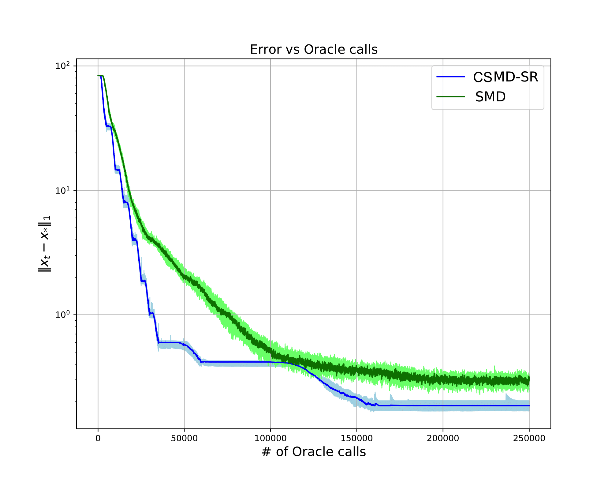
(a) $\kappa_{\Sigma}=1,\sigma=0.1,m_{0}=5000$

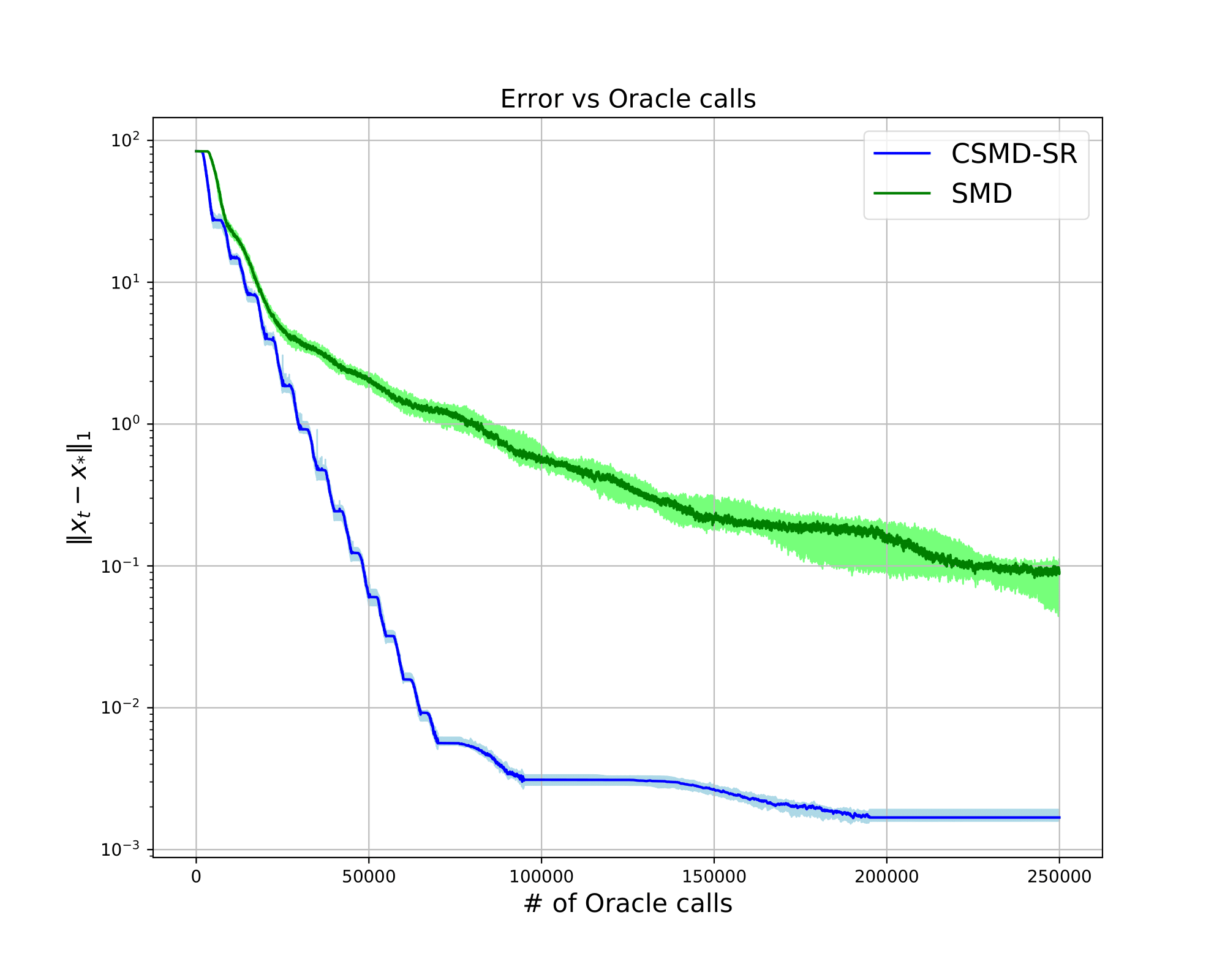
(b) $\kappa_{\Sigma}=1,\sigma=0.001,m_{0}=5000$

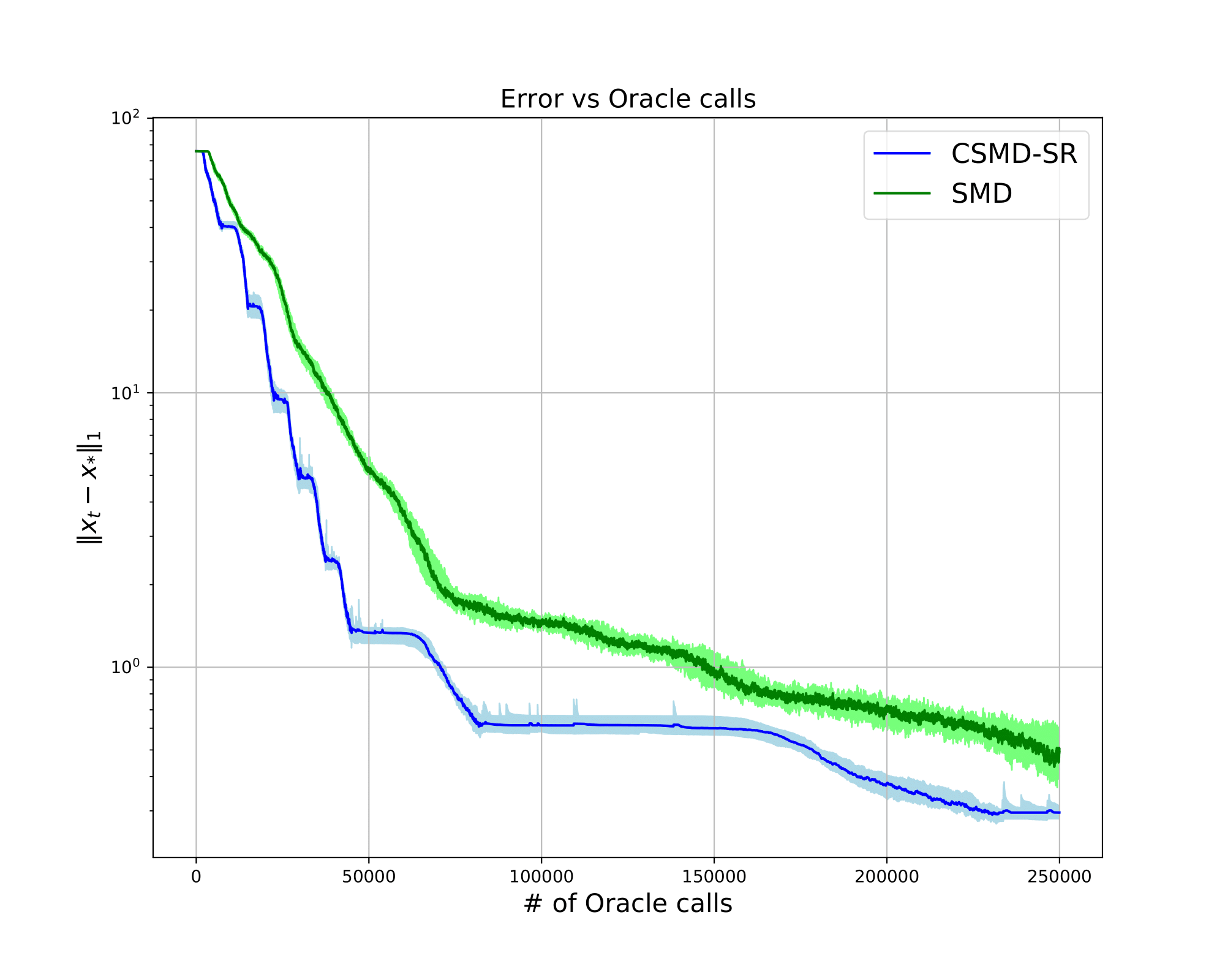
(c) $\kappa_{\Sigma}=0.1,\sigma=0.1,m_{0}=7500$

(d) $\kappa_{\Sigma}=0.1,\sigma=0.001,m_{0}=7500$

Figure 4: CSMD-SR and “vanilla” SMD in Linear Regression problem (activation function $\mathfrak{r}(t)=t$); $\ell_{1}$ error as a function of the number of oracle calls

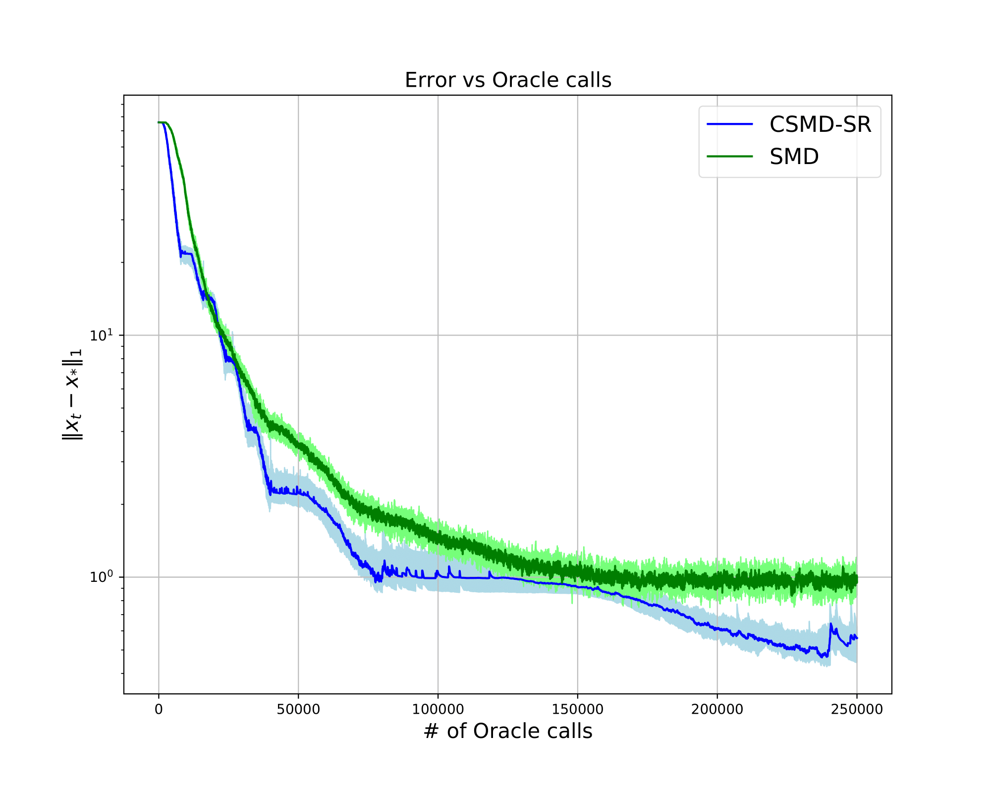
(a) $\kappa_{\Sigma}=1,\sigma=0.1,m_{0}=8000$

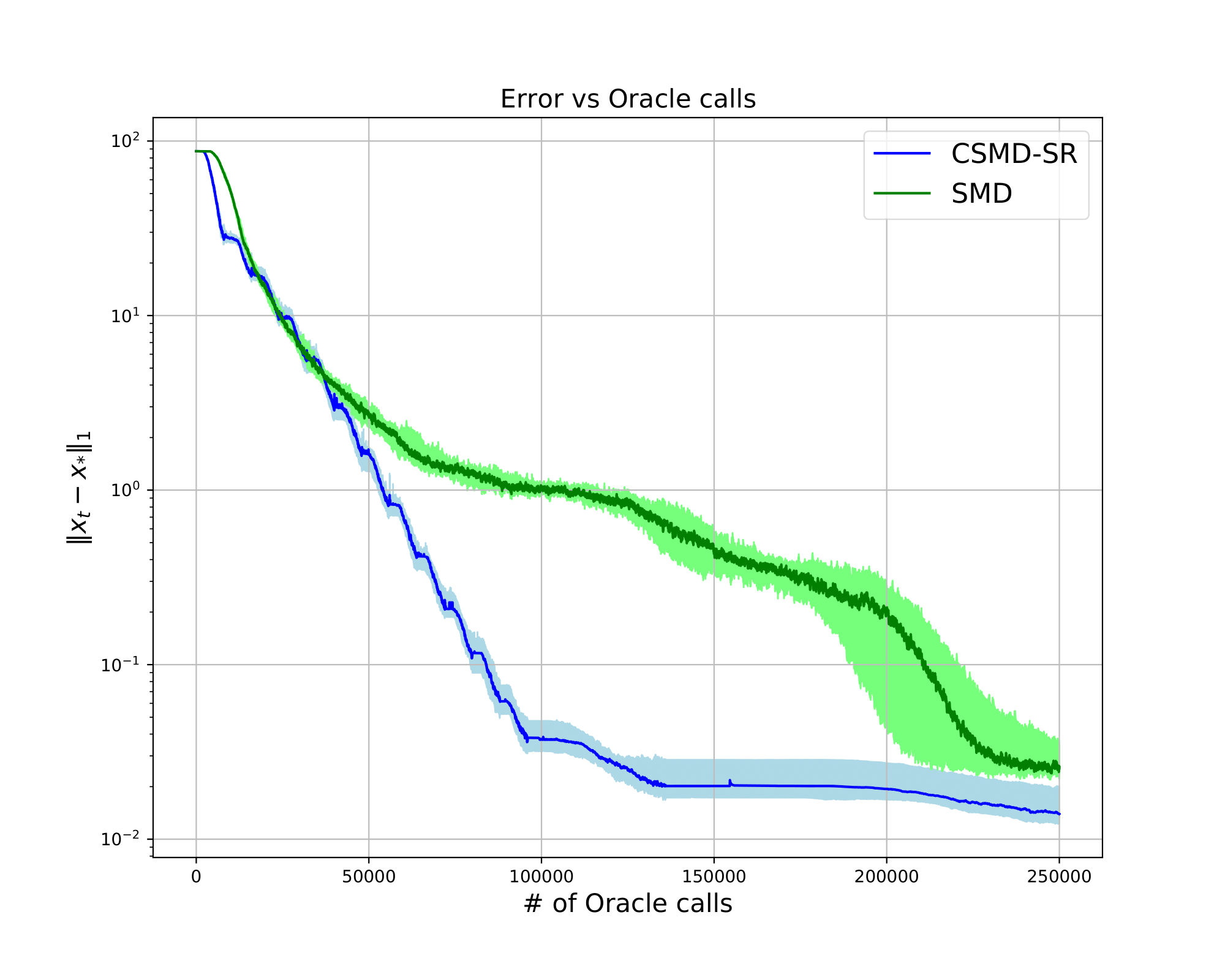
(b) $\kappa_{\Sigma}=1,\sigma=0.001,m_{0}=8000$

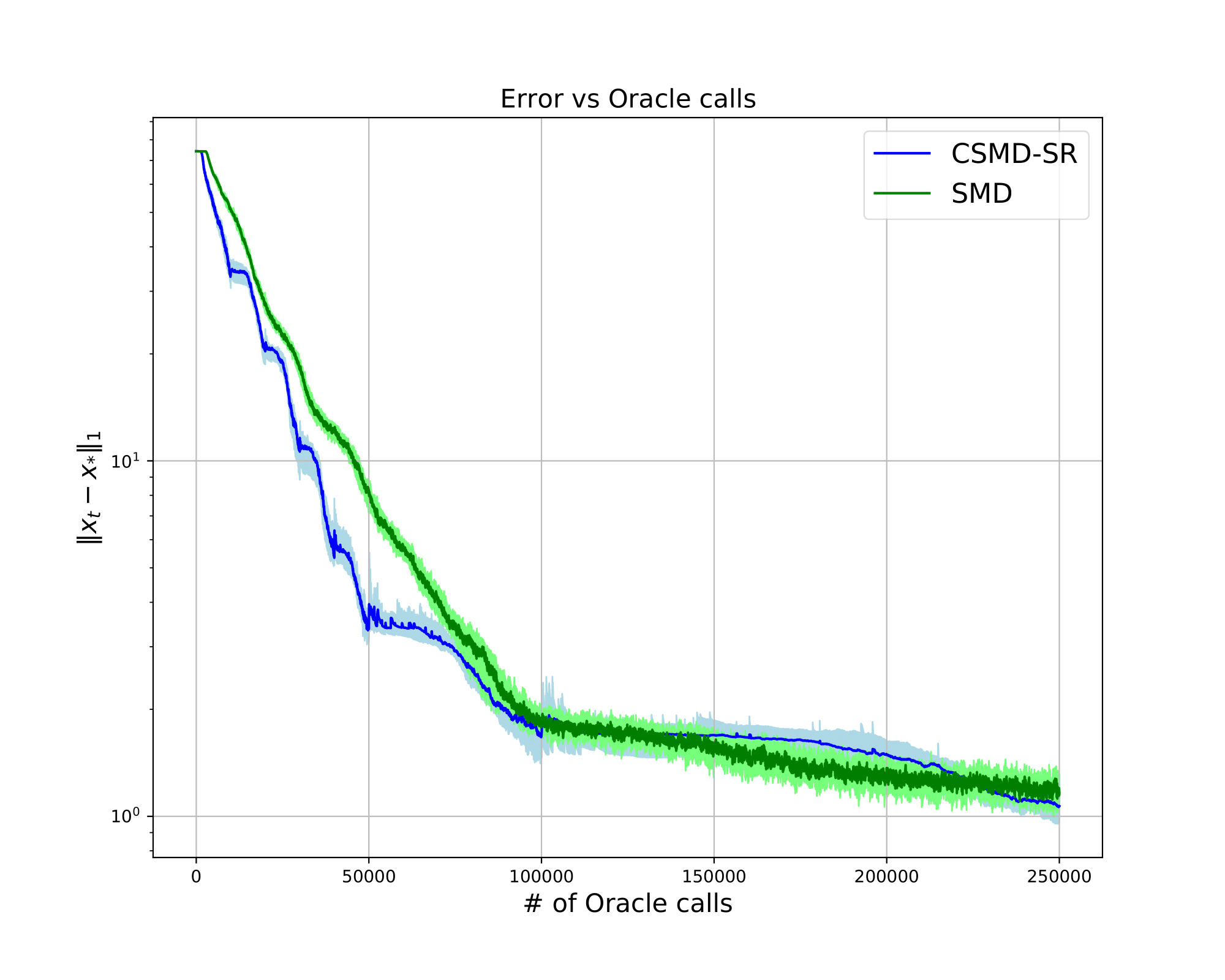
(c) $\kappa_{\Sigma}=0.1,\sigma=0.1,m_{0}=10\,000$

(d) $\kappa_{\Sigma}=0.1,\sigma=0.001,,m_{0}=10\,000$

Figure 5: CSMD-SR and “vanilla” SMD in Generalized Linear Regression problem: activation function $\mathfrak{r}_{1/10}(t)$ ; $\ell_{1}$ error as a function of the number of oracle calls

In our experiments, multistage algorithms exhibit linear convergence on initial iterations. Surprisingly, “standard” (non-Euclidean) SMD also converges fast in the “preliminary” regime. This may be explained by the fact that iteration $x_{i}$ of the SMD obtained by the “usual” proximal mapping $\mathrm{Prox}(\gamma_{i-1}\nabla G(x_{i-1},\omega_{i}),x_{i-1})$ is computed as a solution to the optimization problem with “penalty” $\theta(x)=c\|x\|_{p}^{p}$, $p=1+1/\ln n$ which results in a “natural” sparsification of $x_{i}$. As iterations progress, such “sparsification” becomes insufficient, and the multistage routine eventually outperforms the SMD. Implementing the method for “flatter” nonlinear activation $\mathfrak{r}(t)$ or increased condition number of the regressor covariance matrix $\Sigma$ requires increasing the length $m_{0}$ of the stage of the algorithm.

References

• [1] A. Agarwal, S. Negahban, and M. J. Wainwright. Fast global convergence of gradient methods for high-dimensional statistical recovery. The Annals of Statistics, 40(5):2452 – 2482, 2012.
• [2] A. Agarwal, S. Negahban, and M. J. Wainwright. Stochastic optimization and sparse statistical recovery: Optimal algorithms for high dimensions. In Advances in Neural Information Processing Systems, pages 1538–1546, 2012.
• [3] M. Baes, M. Burgisser, and A. Nemirovski. A randomized mirror-prox method for solving structured large-scale matrix saddle-point problems. SIAM Journal on Optimization, 23(2):934–962, 2013.
• [4] B. Bercu, B. Delyon, and E. Rio. Concentration inequalities for sums and martingales. Springer, 2015.
• [5] P. Bickel, Y. Ritov, and A. Tsybakov. Simultaneous analysis of Lasso and Dantzig selector. The Annals of Statistics, 37(4):1705–1732, 2009.
• [6] L. Birgé, P. Massart, et al. Minimum contrast estimators on sieves: exponential bounds and rates of convergence. Bernoulli, 4(3):329–375, 1998.
• [7] T. Blumensath and M. E. Davies. Iterative hard thresholding for compressed sensing. Applied and computational harmonic analysis, 27(3):265–274, 2009.
• [8] E. Candes, T. Tao, et al. The dantzig selector: Statistical estimation when p is much larger than n. The annals of Statistics, 35(6):2313–2351, 2007.
• [9] E. J. Candes and Y. Plan. A probabilistic and ripless theory of compressed sensing. IEEE transactions on information theory, 57(11):7235–7254, 2011.
• [10] E. J. Candès, Y. Plan, et al. Near-ideal model selection by $\ell_{1}$ minimization. The Annals of Statistics, 37(5A):2145–2177, 2009.
• [11] E. J. Candes, J. K. Romberg, and T. Tao. Stable signal recovery from incomplete and inaccurate measurements. Communications on Pure and Applied Mathematics: A Journal Issued by the Courant Institute of Mathematical Sciences, 59(8):1207–1223, 2006.
• [12] G. Chen and M. Teboulle. Convergence analysis of a proximal-like minimization algorithm using bregman functions. SIAM Journal on Optimization, 3(3):538–543, 1993.
• [13] A. Cohen, W. Dahmen, and R. DeVore. Compressed sensing and best $k$-term approximation. Journal of the American mathematical society, 22(1):211–231, 2009.
• [14] A. Dalalyan and P. Thompson. Outlier-robust estimation of a sparse linear model using $\ell\_1$-penalized Huber’s $m$-estimator. In Advances in Neural Information Processing Systems, pages 13188–13198, 2019.
• [15] X. Fan, I. Grama, and Q. Liu. Hoeffding’s inequality for supermartingales. Stochastic Processes and their Applications, 122(10):3545–3559, 2012.
• [16] R. Foygel Barber and W. Ha. Gradient descent with non-convex constraints: local concavity determines convergence. Information and Inference: A Journal of the IMA, 7(4):755–806, 03 2018.
• [17] P. Gaillard and O. Wintenberger. Sparse accelerated exponential weights. In 20th International Conference on Artificial Intelligence and Statistics (AISTATS), 2017. arXiv preprint arXiv:1610.05022.
• [18] S. Ghadimi and G. Lan. Optimal stochastic approximation algorithms for strongly convex stochastic composite optimization, ii: shrinking procedures and optimal algorithms. SIAM Journal on Optimization, 23(4):2061–2089, 2013.
• [19] L. E. Ghaoui, V. Viallon, and T. Rabbani. Safe feature elimination for the lasso and sparse supervised learning problems. arXiv preprint arXiv:1009.4219, 2010.
• [20] P. Jain, A. Tewari, and P. Kar. On iterative hard thresholding methods for high-dimensional m-estimation. In Advances in Neural Information Processing Systems, pages 685–693, 2014.
• [21] A. Juditsky, F. K. Karzan, and A. Nemirovski. On a unified view of nullspace-type conditions for recoveries associated with general sparsity structures. Linear Algebra and its Applications, 441:124–151, 2014.
• [22] A. Juditsky, F. Kılınç Karzan, and A. Nemirovski. Randomized first order algorithms with applications to $\ell_{1}$-minimization. Mathematical Programming, 142(1):269–310, 2013.
• [23] A. Juditsky, A. Kulunchakov, and H. Tsyntseus. Sparse recovery by reduced variance stochastic approximation. arXiv preprint arXiv:2006.06365, 2020.
• [24] A. Juditsky, A. Nazin, A. Tsybakov, and N. Vayatis. Generalization error bounds for aggregation by mirror descent with averaging. In Advances in neural information processing systems, pages 603–610, 2006.
• [25] A. Juditsky and A. Nemirovski. First order methods for nonsmooth convex large-scale optimization, II: utilizing problems structure. Optimization for Machine Learning, pages 149–183.
• [26] A. Juditsky and A. Nemirovski. Accuracy guarantees for $\ell_{1}$-recovery. IEEE Transactions on Information Theory, 57(12):7818–7839, 2011.
• [27] A. Juditsky and A. Nemirovski. First order methods for nonsmooth convex large-scale optimization, I: general purpose methods. In S. Sra, S. Nowozin, and S. J. Wright, editors, Optimization for Machine Learning. MIT Press Cambridge, 2011.
• [28] A. Juditsky and A. S. Nemirovski. Large deviations of vector-valued martingales in 2-smooth normed spaces. arXiv preprint arXiv:0809.0813, 2008.
• [29] A. Juditsky and Y. Nesterov. Deterministic and stochastic primal-dual subgradient algorithms for uniformly convex minimization. Stochastic Systems, 4(1):44–80, 2014.
• [30] M. Kowalski, P. Weiss, A. Gramfort, and S. Anthoine. Accelerating ista with an active set strategy. In OPT 2011: 4th International Workshop on Optimization for Machine Learning, page 7, 2011.
• [31] B. Laurent and P. Massart. Adaptive estimation of a quadratic functional by model selection. Annals of Statistics, pages 1302–1338, 2000.
• [32] Y. Lei and K. Tang. Stochastic composite mirror descent: Optimal bounds with high probabilities. Advances in Neural Information Processing Systems, 31, 2018.
• [33] H. Liu and R. Foygel Barber. Between hard and soft thresholding: optimal iterative thresholding algorithms. Information and Inference: A Journal of the IMA, 9(4):899–933, 2020.
• [34] J. Mairal. Sparse coding for machine learning, image processing and computer vision. PhD thesis, Cachan, Ecole normale supérieure, 2010.
• [35] L. Meier, S. Van De Geer, and P. Bühlmann. The group lasso for logistic regression. Journal of the Royal Statistical Society: Series B (Statistical Methodology), 70(1):53–71, 2008.
• [36] A. Nemirovski, A. Juditsky, G. Lan, and A. Shapiro. Robust stochastic approximation approach to stochastic programming. SIAM Journal on Optimization, 19(4):1574–1609, 2009.
• [37] A. S. Nemirovski and D. B. Yudin. Complexity of problems and effectiveness of methods of optimization(Russian book). Nauka, Moscow, 1979. Translated as Problem complexity and method efficiency in optimization, J. Wiley & Sons, New York 1983.
• [38] Y. Nesterov. Primal-dual subgradient methods for convex problems. Mathematical programming, 120(1):221–259, 2009.
• [39] Y. Nesterov. Gradient methods for minimizing composite functions. Mathematical programming, 140(1):125–161, 2013.
• [40] Y. Nesterov and A. Nemirovski. On first-order algorithms for $\ell_{1}$/nuclear norm minimization. Acta Numerica, 22:509–575, 2013.
• [41] G. Raskutti, M. J. Wainwright, and B. Yu. Restricted eigenvalue properties for correlated gaussian designs. Journal of Machine Learning Research, 11(Aug):2241–2259, 2010.
• [42] H. Rauhut. Compressive sensing and structured random matrices. Theoretical foundations and numerical methods for sparse recovery, 9(1):92, 2010.
• [43] B. Recht, W. Xu, and B. Hassibi. Null space conditions and thresholds for rank minimization. Mathematical programming, 127(1):175–202, 2011.
• [44] S. Shalev-Shwartz and A. Tewari. Stochastic methods for l1-regularized loss minimization. Journal of Machine Learning Research, 12(Jun):1865–1892, 2011.
• [45] N. Srebro, K. Sridharan, and A. Tewari. Smoothness, low noise and fast rates. In Advances in neural information processing systems, pages 2199–2207, 2010.
• [46] S. Van De Geer and P. Bühlmann. On the conditions used to prove oracle results for the Lasso. Electronic Journal of Statistics, 3:1360–1392, 2009.
• [47] L. Xiao. Dual averaging methods for regularized stochastic learning and online optimization. Journal of Machine Learning Research, 11(88):2543–2596, 2010.