Global Selection of Contrastive Batches via Optimization on Sample Permutations

Abstract

Contrastive Learning has recently achieved state-of-the-art performance in a wide range of unimodal and multimodal tasks. Many contrastive learning approaches use mined hard negatives to make batches more informative during training but these approaches are inefficient as they increase epoch length proportional to the number of mined negatives and require frequent updates of nearest neighbor indices or mining from recent batches. In this work, we provide an alternative to hard negative mining, Global Contrastive Batch Sampling (GCBS), an efficient approximation to the batch assignment problem that upper bounds the gap between the global and training losses, $\mathcal{L}^{Global}-\mathcal{L}^{Train}$, in contrastive learning settings. Through experimentation we find GCBS improves state-of-the-art performance in sentence embedding and code-search tasks. Additionally, GCBS is easy to implement as it requires only a few additional lines of code, does not maintain external data structures such as nearest neighbor indices, is more computationally efficient than the most minimal hard negative mining approaches, and makes no changes to the model being trained. Code is available at https://github.com/vinayak1/GCBS.

1 Introduction

Contrastive Learning is used ubiquitously in training large representation models, such as transformers, and has been shown to achieve state-of-the-art performance in a wide range of unimodal and multimodal tasks across language, vision, code, and audio (Chen et al., 2020a; Gao et al., 2021; Yuxin Jiang & Wang, 2022; Guo et al., 2022; Yu et al., 2022; Radford et al., 2021; Ramesh et al., 2021; Saeed et al., 2021; Yang et al., 2021). In supervised contrastive learning, one is given a paired dataset $(X,Y)$ each with $N$ samples, where $x_{i}\sim y_{i}$ such as similar sentences, code and corresponding language descriptors, or images and their captions. For unsupervised settings, $X,Y$ are alternative ”views” of the same sample often constructed through data augmentation schemes or independent dropout masks (Chen et al., 2020a; Gao et al., 2021). Then batches of rows, $B$, are sampled from this pair of datasets and a model $f(\cdot)$ is trained to concurrently maximize inner products for outputs of similar (positive) data inputs, $f(x_{i})^{T}f(y_{i})$, and minimize inner product for outputs of dissimilar (negative) data inputs $f(x_{i})^{T}f(y_{j}),i,j\in B,i\neq j$.

Due to batch size constraints from hardware limitations, for a fixed batch size $k$, only $Nk$ inner products of the total $N^{2}$ in $f(X)f(Y)^{T}$ are observed in the training loss for each epoch of training. Through the rest of this paper, we will refer to this observed training loss over $Nk$ inner products as $\mathcal{L}^{Train}$ and the total loss over $N^{2}$ inner products as $\mathcal{L}^{Global}$. It has been observed, both in contrastive metric and representation learning (Saunshi et al., 2019; Iscen et al., 2018; Xuan et al., 2020; Mishchuk et al., 2017; Wu et al., 2017; Song et al., 2016; Schroff et al., 2015; Harwood et al., 2017; Ge et al., 2018), that in order for batches to be informative during training, they should be constructed to contain ”hard-negatives”, or large values of $f(x_{i})^{T}f(y_{j}),i\neq j$. Additionally, it has been shown that including hard negatives in batches better approximates global losses (Zhang & Stratos, 2021).

Currently, approaches for constructing batches, and controlling which inner products of the total $N^{2}$ should be used for training, broadly fall into one of two categories. One either uses random sampling or mines nearest neighbors of the reference sample $x_{i}$ in order to greedily insert hard negatives into the same batch as $x_{i}$. While greedily inserting hard negatives is effective in practice (Zhang et al., 2018; Xiong et al., 2021), these methods incur large costs both in time and resources as mining $l<k$ hard negatives per reference sample increases each training epoch by a factor $l$ and often requires maintaining and reranking nearest neighbor indices on expensive accelerated hardware during training. For instance, if $5$ hard negatives from $Y$ are mined for each sample in $X$ during batch construction one will increase the training time of a single epoch by a factor $5$, not including time taken for constructing nearest neighbor indices.

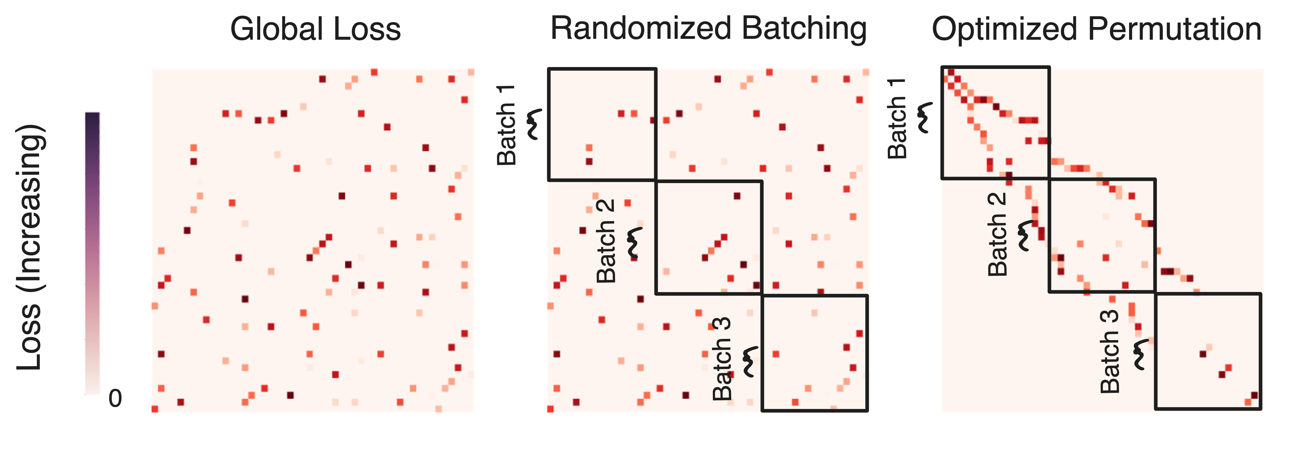
Figure 1: Visualization of inner products of $f(X)f(Y)^{T}$ in global, training with random sampling, and training with permutation optimized sampling for contrastive losses.

Furthermore, hard negative mining often requires frequent reranking to prevent negative anchors from being sampled from stale nearest neighbor indices. Work on momentum based memory banks have found that hard negative mining is especially useful with small lookback intervals (i.e. 2-4 previous batches) (Wang et al., 2021). In this paper, we propose a global alternative to hard negative mining, Global Contrastive Batch Sampling (GCBS), which seeks to efficiently learn a permutation over samples in $X$ and $Y$ to increase the likelihood of hard negatives before each epoch rather than through greedy insertion during training. In Figure 1 above, we visually depict $\mathcal{L}^{Global}$ and $\mathcal{L}^{Train}$ along with the modifications on batches, and therefore the observed loss, for our proposed approach GCBS.

First, we show theoretically that the upper bound on $\mathcal{L}^{Global}-\mathcal{L}^{Train}$, with no oversampling or assumptions on the data/model for commonly used scaled cross entropy losses, such as NT-Xent (Sohn, 2016), are only dependent on batch assignments, total samples $N$, and batch size $k$. We prove that, for fixed $N,k$, this upper bound is minimized as a Quadratic Bottleneck Assignment Problem which seeks to maximize the number of hard negatives in batches by learning a permutation $\pi\in\Pi_{N}$ on the rows of $X$ and $Y$. We then formulate an $\mathcal{\tilde{O}}(N^{2})$ approximation for optimizing over this permutation, GCBS, and show that it is more efficient than any hard negative mining approaches, even for $l=1$, per training epoch. We analyze the loss behavior of GCBS and show that GCBS better approximates the total contrastive loss. Lastly, we empirically evaluate GCBS in the context of supervised contrastive finetuning for sentence embedding (STS) and code search (CosQA, AdvTest, CodeSearchNet) and achieve state-of-the-art performance for all of these tasks.

In this work, we summarize our contributions as follows:

1. We prove that the upper bound of the gap between the total and observed losses in contrastive learning for a fixed batch size $B$ without oversampling, $\mathcal{L}^{Global}-\mathcal{L}^{Train}$, is constrained by a Quadratic Bottleneck Assignment Problem and can be relaxed to a Matrix Bandwidth Minimization problem.

2. We formulate a $\mathcal{\tilde{O}}(N^{2})$ time and $\mathcal{O}(Nk)$ space complexity approximation to the Matrix Bandwidth Minimization problem, GCBS, using the Cuthill-Mckee heuristic and implement this algorithm in less than 50 lines of PyTorch.

3. We analyze the loss behavior of GCBS and show that, in sentence embedding and code-search tasks, GCBS better approximates the total contrastive loss.

4. We empirically evaluate GCBS and achieve state-of-the-art performance on the STS taskset for sentence embeddings. Additionally, we achieve state-of-the-art performance for the CosQA, AdvTest, and CodeSearchNet tasks for joint programming language-natural language embeddings.

The rest of this paper is organized as follows. In Section 2 we discuss related work. In Section 3, we derive upper bounds on the gap between total and observed losses and in Section 4 formulate these bounds as Quadratic Assignment Problems. In Section 5, we relax our QBAP to a Matrix Bandwidth Minimization problem, introduce our proposed method, GCBS, for approximating global contrastive losses, and provide implementation details. In Section 6, we provide experimental results for sentence embedding and code search tasks using GCBS. Section 7 provides discussion and Section 8 concludes the paper.

2 Related Work

2.1 Contrastive Representation Learning

Contrastive Learning has been used ubiquitously for vision, language, and audio representation learning. In vision tasks, SimCLR (Chen et al., 2020a) showed that using augmented views of the same image as positive samples and the NT-Xent objective (Sohn, 2016) improves performance of unsupervised classification. MoCo (He et al., 2020; Chen et al., 2020b) used memory banks of negative samples from recent batches to increase the effective contrastive batch size, and Sylvain et al. (2020); Khosla et al. (2020) show improvements using supervised contrastive frameworks. For sentence embedding tasks, contrastive learning has been used both in pretraining (Logeswaran & Lee, 2018), finetuning and continuous prompt tuning settings (Gao et al., 2021; Yuxin Jiang & Wang, 2022) to provide state-of-the-art performance. Additionally, contrastive learning has been used extensively to align representations across different modalities for downstream use in multimodal tasks such as those involving language/code, language/vision, and vision/decision making (Guo et al., 2022; Feng et al., 2020; Guo et al., 2021; Radford et al., 2021; Ramesh et al., 2021; Laskin et al., 2020).

2.2 Hard Negative Mining in Metric and Contrastive Learning

Selection of hard negatives during batch construction is well-studied and has been shown, both theoretically and empirically, to improve metric and contrastive learning (Saunshi et al., 2019; Iscen et al., 2018; Xuan et al., 2020; Mishchuk et al., 2017; Wu et al., 2017). Prior work in metric learning (Song et al., 2016; Schroff et al., 2015; Harwood et al., 2017; Ge et al., 2018) has observed that ”hard negatives”, or negatives which are difficult to discriminate against with respect to a particular query’s embedding, are beneficial for downstream classifier performance. In contrastive learning, Zhang et al. (2018) uses Mixup to generate hard negatives in latent space. Chuang et al. (2020) proposes a debiased contrastive loss which approximates the underlying “true” distribution of negative examples and Yang et al. (2022) studies the effect of restricting negative sampling to regions around the query using a variational extension to the InfoNCE objective. In Kim et al. (2020); Ho & Nvasconcelos (2020) adversarial examples are used to produce more challenging positives and hard negatives. In Xiong et al. (2021), nearest neighbor indices and a secondary model from prior checkpoints are used to mine hard negatives for text retrieval tasks.

Robinson et al. (2021) reweights negative samples based on their Euclidean distance and debiases positive samples in order to control the level of difficulty in unsupervised contrastive learning. Kalantidis et al. (2020) show that harder negative examples are needed to improve performance and training speed in vision tasks and propose adding ”synthetic” hard negatives in training batches using convex combinations of nearest neighbors.

2.3 Quadratic Assignment Problems

The Quadratic Assignment Problem (QAP), stemming from facilities locations problems (Koopmans & Beckmann, 1957), in combinatorial optimization seeks to minimize the total cost of assigning $n$ facilities to $n$ locations. Formally, one seeks to optimize $\min_{\pi\in\Pi_{n}}\operatorname{Tr}(W\pi D\pi^{T})$ over $\Pi_{n}$, the set of $n\times n$ permutation matrices, for a given cost matrix $W\in\mathbb{R}^{n\times n}$ and distance matrix $D\in\mathbb{R}^{n\times n}$. The Quadratic Bottleneck Assignment Problem (QBAP) (Steinberg, 1961) takes a similar form but minimizes the maximum cost rather than the total cost, $\min_{\pi\in\Pi_{n}}\max_{i,j}(W\pi D\pi^{T})_{i,j}$. The Graph Bandwidth Minimization Problem, seeks to minimize the dispersion of nonzero costs from the main diagonal for a sparse distance matrix $D$ and is a special case of QBAP in which the cost matrix $W$ increases monotonically in $|i-j|$. In this paper, we prove that minimizing the upper bound between the total and the observed training losses $\mathcal{L}^{Global}-\mathcal{L}^{Train}$ over a pair of datasets $X,Y$ is bounded by Quadratic Assignment Problems and approximated by a Graph Bandwidth Minimization Problem. This connection is shown visually in Figure 1. As all of the aforementioned problems are NP-Hard, we utilize the Cuthill-McKee algorithm (Cuthill & McKee, 1969), a $\mathcal{\tilde{O}}(N^{2})$ approximation for bandwidth minimization.

3 Global and Training Losses for Cross-Entropy based Contrastive Objectives

In this section, we characterize the gap between training and global losses in supervised contrastive learning for the Normalized Temperature-scaled Cross Entropy (NT-Xent) loss (Sohn, 2016). The NT-Xent loss is a ubiquitous contrastive objective used in state-of-the-art models for sentence embedding, code-language tasks and vision-language tasks (Gao et al., 2021; Yuxin Jiang & Wang, 2022; Guo et al., 2022; Chen et al., 2020a; Radford et al., 2021).

Let $X,Y\in\mathbb{R}^{n\times d}$ be the output representations for two paired datasets each with $N$ samples. Consider a supervised setting where $x_{i},y_{i}$ are considered ”positive” pairs and $x_{i},y_{j}$ are considered negative pairs $\forall i\neq j$. Note that the analysis we provide can be modified to incorporate multiple positives, such as those from class information, which will have tighter bounds in terms of the number of samples $N$ and the batch size $k$. Additionally, let $\tau\in\mathbb{R}_{+}$ be a tunable temperature parameter which scales logit values in the objective. When $\tau$ is small, the NT-Xent loss is a proxy for the hard maximum loss. Assume that all representations have been normalized, that is $\|x_{i}\|_{2},\|y_{i}\|_{2},=1$ $\forall i$.

3.1 The Global and Training NT-Xent objectives, $\mathcal{L}^{Global}$ and $\mathcal{L}^{Train}$

First, we provide the contrastive loss over all $N^{2}$ pairs of inner products between $X$ and $Y$. We call this the global objective as it contains all pairwise contrastive information and, in the absence of resource constraints, is the loss one would seek to minimize. The Global NT-Xent objective is given as follows:

Definition 3.1 (Global NT-Xent objective).

The Global NT-Xent objective is given as follows: $\begin{aligned} \mathcal{L}^{Global}&=-\frac{1}{N}\sum_{i=1}^{N}\log\frac{\exp(x_{i}^{T}y_{i}{\tau}^{-1})}{\sum_{\begin{subarray}{c}j=1\end{subarray}}^{N}\exp(x_{i}^{T}y_{j}{\tau}^{-1})}.\\ &=\frac{1}{N}\sum_{i=1}^{N}\bigl{(}-x_{i}^{T}y_{i}\tau^{-1}+\log\sum_{\begin{subarray}{c}j=1\end{subarray}}^{N}\exp(x_{i}^{T}y_{j}{\tau}^{-1})\bigr{)}.\end{aligned}$

Due to memory constraints, during training one does not make all $N^{2}$ comparisons over pairs in $X$ and $Y$ during a training epoch. Instead, each sample $x_{i}$ is only contrasted against $k$ in-batch samples in $Y$, its positive anchor $y_{i}$ and $k-1$ negative anchors. This observed training loss will be strictly less than the global loss as it makes $k$ comparisons out of $N$ total for each sample. For a fixed batch assignment $B$, let $B_{i}$ be the indices of rows in $Y$ contained in a batch with $x_{i}$. The training NT-Xent objective is given as follows:

Definition 3.2 (Training NT-Xent objective).

The Training NT-Xent objective is given as follows: $\begin{aligned} \mathcal{L}^{Train}&=-\frac{1}{N}\sum_{i=1}^{N}\log\frac{\exp(x_{i}^{T}y_{i}{\tau}^{-1})}{\sum_{\begin{subarray}{c}j\in B_{i}\end{subarray}}\exp(x_{i}^{T}y_{j}{\tau}^{-1})}.\\ &=\frac{1}{N}\sum_{i=1}^{N}\bigl{(}-x_{i}^{T}y_{i}\tau^{-1}+\log\sum_{\begin{subarray}{c}j\in B_{i}\end{subarray}}\exp(x_{i}^{T}y_{j}{\tau}^{-1})\bigr{)}.\end{aligned}$

3.2 Minimizing the gap between $\mathcal{L}^{Global}$ and $\mathcal{L}^{Train}$

For a fixed set of batches $B$, we will first provide upper bounds on $\mathcal{L}^{Global}$ and lower bounds on $\mathcal{L}^{Train}$ using Log-Sum-Exp properties (Calafiore & El Ghaoui, 2014). Using the upper bound for Log-Sum-Exp, the following bound on $\mathcal{L}^{Global}$ can be obtained where equivalence is attained when all inner products have the same value.

3.2.1 Upper bound on $\mathcal{L}^{Global}$

Lemma 3.3 (Upper bound on $\mathcal{L}^{Global}$).

With Log-Sum-Exp properties (Calafiore & El Ghaoui, 2014), $\mathcal{L}^{Global}$ with the NT-Xent contrastive objective can be upper bounded as: $\begin{aligned} \mathcal{L}^{Global}&=\frac{1}{N}\sum_{i=1}^{N}-x_{i}^{T}y_{i}\tau^{-1}+\log\sum_{\begin{subarray}{c}j=1\end{subarray}}^{N}\exp(x_{i}^{T}y_{j}{\tau}^{-1})\\ &\leq\frac{1}{N}\sum_{i=1}^{N}-x_{i}^{T}y_{i}\tau^{-1}+\log(N\max_{j}\exp(x_{i}^{T}y_{j}{\tau}^{-1})\\ &=\frac{1}{N}\sum_{i=1}^{N}{\tau}^{-1}(-x_{i}^{T}y_{i}{\tau}^{-1}+\max_{j}x_{i}^{T}y_{j})+\log N.\end{aligned}$

3.2.2 Lower Bounds on $\mathcal{L}^{Train}$

Two lower bounds can be derived for $\mathcal{L}^{Train}$, first using the translation identity property (Nielsen & Sun, 2016) and then using the standard lower bound for Log-Sum-Exp (Calafiore & El Ghaoui, 2014).

Lemma 3.4 (First lower bound on $\mathcal{L}^{Train}$ using Translation Identity).

With the Log-Sum-Exp translation identity property (Nielsen & Sun, 2016), $\mathcal{L}^{Train}$ with the NT-Xent contrastive objective can be bounded as: $\begin{aligned} \mathcal{L}^{Train}&=\frac{1}{N}\sum_{i=1}^{N}-x_{i}^{T}y_{i}\tau^{-1}+\log\sum_{\begin{subarray}{c}j\in B_{i}\end{subarray}}\exp(x_{i}^{T}y_{j}{\tau}^{-1})\\ &\geq\frac{1}{N}\sum_{i=1}^{N}-x_{i}^{T}y_{i}\tau^{-1}+\log(k\min_{j\in B_{i}}\exp(x_{i}^{T}y_{j}{\tau}^{-1}))\\ &=\frac{1}{N}\sum_{i=1}^{N}{\tau}^{-1}(-x_{i}^{T}y_{i}+\min_{j\in B_{i}}x_{i}^{T}y_{j})+\log k.\end{aligned}$

Lemma 3.5 (Second lower bound on $\mathcal{L}^{Train}$ using standard Log-Sum-Exp bound).

With Log-Sum-Exp properties (Calafiore & El Ghaoui, 2014), $\mathcal{L}^{Train}$ with the NT-Xent contrastive objective can be bounded as:

$\begin{aligned} \mathcal{L}^{Train}&=\frac{1}{N}\sum_{i=1}^{N}-x_{i}^{T}y_{i}\tau^{-1}+\log\sum_{\begin{subarray}{c}j\in B_{i}\end{subarray}}\exp(x_{i}^{T}y_{j}{\tau}^{-1})\\ &\geq\frac{1}{N}\sum_{i=1}^{N}-x_{i}^{T}y_{i}\tau^{-1}+\log(\max_{j\in B_{i}}\exp(x_{i}^{T}y_{j}{\tau}^{-1}))\\ &=\frac{1}{N}\sum_{i=1}^{N}{\tau}^{-1}(-x_{i}^{T}y_{i}\tau^{-1}+\max_{j\in B_{i}}x_{i}^{T}y_{j}).\end{aligned}$

3.2.3 Upper bounds on $\mathcal{L}^{Global}-\mathcal{L}^{Train}$

We can now bound the gap between the global and training losses of the NT-Xent objective for a fixed batch set of batches $B$. The diagonal terms are included in both the global and training losses and will therefore not factor into characterizing the gap.

Theorem 3.6 (First upper bound on $\mathcal{L}^{Global}-\mathcal{L}^{Train}$).

An upper bound on $\mathcal{L}^{Global}-\mathcal{L}^{Train}$ for the NT-Xent objective using the lower bound from Lemma 3.4 is: $\begin{aligned} \mathcal{L}^{Global}-\mathcal{L}^{Train}\leq\frac{1}{N}\sum_{i=1}^{N}&{\tau}^{-1}(\max_{j}x_{i}^{T}y_{j}-\min_{j\in B_{i}}x_{i}^{T}y_{j})\\ &+\log\frac{N}{k}.\end{aligned}$

Theorem 3.7 (Second upper bound on $\mathcal{L}^{Global}-\mathcal{L}^{Train}$).

An upper bound on $\mathcal{L}^{Global}-\mathcal{L}^{Train}$ for the NT-Xent objective using the lower bound from Lemma 3.5 is: $\begin{aligned} \mathcal{L}^{Global}-\mathcal{L}^{Train}\leq\frac{1}{N}\sum_{i=1}^{N}&{\tau}^{-1}(\max_{j}x_{i}^{T}y_{j}-\max_{j\in B_{i}}x_{i}^{T}y_{j})\\ &+\log N.\end{aligned}$

4 Minimizing $\mathcal{L}^{Global}-\mathcal{L}^{Train}$ as Quadratic Assignment over Batches

Note that from Theorems 3.6 and 3.7 we have bounded the gap between $\mathcal{L}^{Global}-\mathcal{L}^{Train}$ without making any assumptions on data distribution or models. Additionally, we can see that the bounds are dependent on the batch assignments $j\in B_{i}$, batch size $k$, and total number of samples $N$. Note the losses we have characterized have been summed over samples in $X$ which we will denote as $\mathcal{L}^{Global}_{X},\mathcal{L}^{Train}_{X}$ and consider losses summed over samples in $Y$ as $\mathcal{L}^{Global}_{Y},\mathcal{L}^{Train}_{Y}$.

4.1 Batches assignment as optimization over row permutations

We will now rewrite our optimization problems over permutations $\pi\in\Pi_{N}$ instead of sets of batch assignments $\{B\}$, an equivalent formulation. First, recognize that our bounds are dependent only on batch assignments of negatives $j\in B_{i}$. Without loss of generality assume that batches are constructed sequentially after applying a row permutation $\pi\in\Pi_{N}$ on $X$ and $Y$. That is, batches are constructed over $\pi(X),\pi(Y)$ such that $j\in B_{i}\iff\lfloor\frac{j}{k}\rfloor=\lfloor\frac{i}{k}\rfloor$. Recognize that this batch construction can be written as a block diagonal matrix of the form $A\in\{0,1\}^{N\times N}$ and $A_{i,j}=1$ if $\lfloor\frac{j}{k}\rfloor=\lfloor\frac{i}{k}\rfloor$. Note this sequential constraint is not restrictive as it accommodates all possible batch assignments on $X,Y$ with the appropriate permutation $\pi\in\Pi_{N}$. When introducing a fixed sequential batching, we can rewrite the minimizer of the upper bound on $\mathcal{L}^{Global}-\mathcal{L}^{Train}$ from Theorems 3.6 and 3.7 as an optimization problem over permutations $\pi\in\Pi_{N}$ on $X,Y$ rather than explicitly on $\{B\}$. The form of these optimizations problems are the Quadratic Bottleneck Assignment Problem and the Quadratic Assignment Problem (Koopmans & Beckmann, 1957). These are well-known NP-Hard combinatorial optimization problems and in the following two sections we will discuss formulation and efficient approximations.

4.2 Bounds related to Quadratic Bottleneck Assignment Problems

The upper bound in Theorem 3.6, for the sum $(\mathcal{L}^{Global}_{X}-\mathcal{L}^{Train}_{X})+(\mathcal{L}^{Global}_{Y}-\mathcal{L}^{Train}_{Y})$, is minimized when the smallest inner product over in-batch negatives is maximized over $\pi\in\Pi_{N}$. Denote $Z_{ij}\triangleq\min\{x_{i}^{T}y_{j},y_{i}^{T}x_{j}\}$ and $\odot$ as the Hadamard product. This is a QBAP, the proof of which is deferred to Appendix A.1, as we are interested in the minimizing the maximum value of the elementwise product of two symmetric matrices $\pi Z\pi^{T}$ and $A$.

Theorem 4.1 (Formulation of QBAP for bound in Theorem 3.6).

The following Quadratic Bottleneck Assignment Problem, minimizes the upper bound provided in Theorem 3.6 summed over $X$ and $Y$:

$$\boxed{\min_{\pi\in\Pi_{N}}\max_{i,j}-A\odot\pi Z\pi^{T}.}$$

4.3 Bounds related to Quadratic Assignment Problems

The upper bound in Theorem 3.7, for the sum $(\mathcal{L}^{Global}_{X}-\mathcal{L}^{Train}_{X})+(\mathcal{L}^{Global}_{Y}-\mathcal{L}^{Train}_{Y})$, is minimized when the sum of inner products over in-batch negatives is maximized over permutations $\pi\in\Pi_{N}$. This can be formulated equivalently as either the Frobenius inner product between the symmetric matrices $\pi(XY^{T}+YX^{T})\pi^{T}$ and $A$ or the Trace of their product. These are QAPs, the proof of which is deferred to Appendix A.2.

Theorem 4.2 (Formulation of QAP for bound in Theorem 3.7).

The following Quadratic Assignment Problem minimizes the upper bound in Theorem 3.7:

$$\boxed{\max_{\pi\in\Pi_{N}}Tr(A\pi(XY^{T}+YX^{T})\pi^{T}).}$$

Heuristics for both the QAP and QBAP in $\mathcal{O}(N^{3})$ and $\tilde{\mathcal{O}}(N^{2})$ time complexity respectively are well-known (Kuhn, 1955; Munkres, 1957; Edmonds & Karp, 1972; Jonker & Volgenant, 1988; Cuthill & McKee, 1969). In the next section, we will formulate approximate solutions to the QBAP in Theorem 4.1 with $\mathcal{O}(Nk)$ space and $\tilde{\mathcal{O}}(N^{2})$ time complexity.

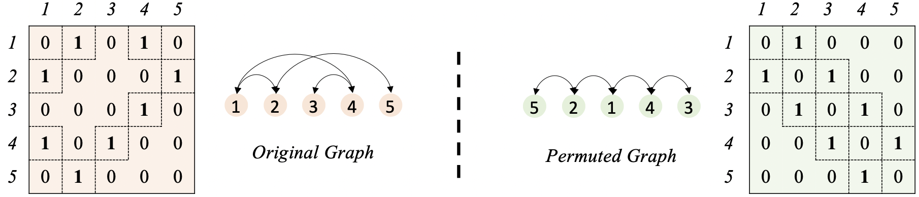
Figure 2: Visual depiction of connection between minimizing graph and matrix bandwidths.

5 Global Contrastive Batch Sampling: Efficient approximations to the QBAP with Cuthill-McKee

In practice, when $N$ is large it can be difficult to hold $XY^{T}$ in memory and approximation algorithms for the QAP problem (Kuhn, 1955; Munkres, 1957; Edmonds & Karp, 1972; Jonker & Volgenant, 1988) have $\mathcal{O}(N^{3})$ complexity. Therefore, in optimizing over $\pi\in\Pi_{N}$ we will make two modifications in order to develop a $\mathcal{O}(Nk)$ space and $\tilde{\mathcal{O}}(N^{2})$ worst-case time complexity approximation to the QBAP in Theorem 4.1. First, we will sparsify the matrix $XY^{T}$ on a quantile $q$ which censors values below the quantile to $0$. Secondly, we use an $\mathcal{\tilde{O}}(N^{2})$ matrix bandwidth minimization heuristic commonly used for sparse matrix multiplication and decomposition (Cuthill & McKee, 1969) to efficiently attain an assignment over sample permutations.

5.1 Approximating the QBAP: Sparsification and Matrix Bandwidth Minimization

Previous literature (Burkard, 1984) has shown the QBAP and Matrix Bandwidth Minimization Problem to be equivalent when the cost matrix is increasing in $|i-j|$ and (Burkard, 1984) proposes thresholding in order to reduce coefficients in the matrix $XY^{T}$. First, we sparsify $XY^{T}$ on a threshold quantile $q$ as follows:

$$(\tilde{XY}^{T})_{i,j}=\left\{\begin{aligned} 1,&\qquad&x_{i}^{T}y_{j}>q,i\neq j\\ 0,&&else.\end{aligned}\right.$$

Note that there exists a minimal quantile $q^{*}$ which constructs a sparse matrix $\tilde{XY}^{T}$ that achieves the same solution as the dense matrix $XY^{T}$. This is due to the fact that since we are interested in maximizing the minimum inner product over in-batch negatives, the smallest values of $XY^{T}$ in each row are not of interest for the batch assignment objective.

5.2 Approximating the QBAP: Cuthill-McKee Algorithm

Algorithm 1 Cuthill-Mckee algorithm on sparse graph

0:  Sparse Adjacency Matrix $G\in\{0,1\}^{N\times N}$

  (1) Get peripheral vertex $v_{i}$ with lowest degree from the vertices in $G$. Set $\pi=[v_{i}]$. $\mathbf{Time\hskip 5.69054ptCompl.:\mathcal{O}(|E|)=\mathcal{O}((1-q)N^{2})\approx\mathcal{O}(kN)}$

  (2) Perform Breadth First Search on the Graph $G$ rooted at $v_{i}$ excluding elements in $\pi$. $\mathbf{Time\hskip 5.69054ptCompl.:\mathcal{O}(N)}$

  (3) Label each vertex, other than $v_{i}$, on their distance from $v_{i}$, creating ”levels”. $\mathbf{Time\hskip 5.69054ptCompl.:\mathcal{O}(N)}$

  (4) Order vertices by level, tiebreaker of ascending vertex degree and append the first item to $\pi$. $\mathbf{Time\hskip 5.69054ptCompl.:\mathcal{O}(Nlog(N))}$

  (5) If $|\pi|<N$, return to Step (2) and repeat this process with the most recently added vertex as the root.

  (6) Return permutation $\pi=[i_{0},i_{1},\dots,i_{n}]$

On this sparsified matrix $\tilde{XY}^{T}$, we should seek to maximize the number of nonzero values in $\pi(\tilde{XY}^{T}+(\tilde{XY}^{T})^{T})\pi^{T}\odot A$ to minimize the upper bound in 4.1. The QBAP formulations and the Matrix Bandwidth Minimization problem are approximately equivalent due to the fixed sequential batching which assigns batches along the main diagonal of $\pi XY^{T}\pi^{T}$. Since $\{B\}$ is comprised of blocks on the main diagonal, minimizing the dispersion of non-zero entries, after sparsification, from the main diagonal will maximize the probability of large inner product values within batches. As a result, our algorithm for minimizing $(\mathcal{L}^{Global}_{X}-\mathcal{L}^{Train}_{X})+(\mathcal{L}^{Global}_{Y}-\mathcal{L}^{Train}_{Y})$, GCBS, is an $\mathcal{\tilde{O}}(N^{2})$ relaxation to the bound in Theorem 4.1. In Algorithm 1 we detail the Cuthill-Mckee algorithm for matrix bandwidth minimization (Cuthill & McKee, 1969) along with worst case runtimes for each step.

Additionally, we note that the Cuthill-Mckee algorithm has been extensively applied in graph bandwidth problems. In the directed unweighted graph setting, a linear graph arrangement (Feige, 2000) is applied on an adjacency matrix $G\in\{0,1\}^{N\times N}$ such that each node is placed at the corresponding row integer value $i$ on the x-axis with edges to nodes $j$ if $G_{ij}\neq 0$. The objective in this case is to minimize the length of the longest edge. By viewing the batch assignment problem in this graphical setting, one can recognize that in our sparse implementation GCBS seeks to minimize the distance between nodes $i,j$ where $x_{i}^{T}y_{j}$ is a relatively large inner product. This connection between minimizing graph and matrix bandwidths is shown visually in Figure 2.

Model	CosQA	AdvTest	Ruby	JS	Go	Python	Java	PHP	CSN Avg
RoBERTa	60.3	18.3	58.7	51.7	85.0	58.7	59.9	56.0	61.7
CodeBERT	65.7	27.2	67.9	62.0	88.2	67.2	67.6	62.8	69.3
GraphCodeBERT	68.4	35.2	70.3	64.4	89.7	69.2	69.1	64.9	71.3
SYNCoBERT	-	38.3	72.2	67.7	91.3	72.4	72.3	67.8	74.0
PLBART	65.0	34.7	67.5	61.6	88.7	66.3	66.3	61.1	68.5
CodeT5-base	67.8	39.3	71.9	65.5	88.8	69.8	68.6	64.5	71.5
UniXcoder	70.1	41.3	74.0	68.4	91.5	72.0	72.6	67.6	74.4
- with GCBS	71.1 (+1.0)	43.3 (+2.0)	76.7	70.6	92.4	74.6	75.3	70.2	76.6 (+2.2)

Table 1: The performance comparison of supervised models along with a comparison of the best performing model (UniXcoder) (Guo et al., 2022) when using GCBS vs the standard Random Sampling. The reported score is Mean Reciprical Rank magnified by a factor of 100. GCBS improves previous best MRR when used with UniXcoder by 2.2 points achieving new state-of-the-art results (Row shaded gray).

Model	STS12	STS13	STS14	STS15	STS16	STS-B	SICK-R	Avg
SBERTbase	70.97	76.53	73.19	79.09	74.30	77.03	72.91	74.89
SBERTbase-flow	69.78	77.27	74.35	82.01	77.46	79.12	76.21	76.60
SBERTbase-whitening	69.65	77.57	74.66	82.27	78.39	79.52	76.91	77.00
ConSERT-BERTbase	74.07	83.93	77.05	83.66	78.76	81.36	76.77	79.37
SimCSE-BERTbase	75.30	84.67	80.19	85.40	80.82	84.25	80.39	81.57
- with GCBS	75.81	85.30	81.12	86.58	81.68	84.80	80.04	82.19 (+0.62)
PromCSE-BERTbase	75.96	84.99	80.44	86.83	81.30	84.40	80.96	82.13
- with GCBS	75.20	85.00	81.00	86.82	82.55	84.76	79.95	82.18 (+0.05)
SimCSE-RoBERTabase	76.53	85.21	80.95	86.03	82.57	85.83	80.50	82.52
- with GCBS	76.94	85.64	81.87	86.84	82.78	85.87	80.68	82.95 (+0.43)
PromCSE-RoBERTabase	77.51	86.15	81.59	86.92	83.81	86.35	80.49	83.26
- with GCBS	77.33	86.77	82.19	87.57	84.09	86.78	80.05	83.54 (+0.28)
SimCSE-RoBERTalarge	77.46	87.27	82.36	86.66	83.93	86.70	81.95	83.76
- with GCBS	78.90	88.39	84.18	88.32	84.85	87.65	81.27	84.79 (+1.03)
PromCSE-RoBERTalarge	79.56	88.97	83.81	88.08	84.96	87.87	82.43	85.10
- with GCBS	80.49	89.17	84.57	88.61	85.38	87.87	81.49	85.37 (+0.27)

Table 2: The performance comparison of supervised models along with a comparison of the best performing models, SimCSE (Gao et al., 2021) and PromCSE (Yuxin Jiang & Wang, 2022), with and without GCBS. The reported score is Spearman correlation magnified by a factor of 100. For RoBERTa_large backbone models, GCBS improves previous best Spearman correlation when used with SimCSE by 1.03 points and PromCSE by 0.27 points achieving new state-of-the-art results.

6 Experimentation

In this section, we detail experiments for sentence embedding and code-search tasks when using GCBS instead of the standard Random Sampling. We find that GCBS improves state-of-the-art performance for both tasks while requiring minimal code changes. Specification of hyperparameters are included in Appendix Section H.

6.1 Code Search Experiments

Semantic code search is an important problem in representation learning that jointly embeds programming and natural languages (Husain et al., 2019). In this task, one is concerned with returning relevant code when given a natural language query. This is a problem of great interest due to the potential for aiding programmers when developing code and possesses challenges in aligning highly technical and abbreviated language with the programming language modality. Recently, models for this task have been improved using contrastive learning (Guo et al., 2022) by enforcing sequence embeddings for code and their corresponding natural language comments to have large inner products relative to unrelated natural language comments. GCBS provides further gains and achieves state-of-the-art performance when used with well-performing contrastive learning models, UniXcoder (Guo et al., 2022) as shown in Table 1.

6.2 Sentence Embedding Experiments

Recently, contrastive learning approaches, which enforce that pretrained sentence embeddings for mined pairs of similar sentences have large inner products relative to the inner products of random pairs of sentences, have provided state of the art performance for sentence embedding tasks. GCBS provides further gains and achieves state-of-the-art performance when used with well-performing contrastive learning models, SimCSE (Gao et al., 2021) and PromCSE (Yuxin Jiang & Wang, 2022), as shown in Table 2

6.3 Self-Supervised Image Classification Experiments

Additionally, we conduct experiments on vision datasets with strong and extensive self-supervised image classification baselines across a variety of methods from past literature. In particular, we evaluate on the Imagenette and Cifar10 vision classification datasets obtained from Lightly AI .

On these tasks, we find GCBS to be beneficial when implemented both with Moco (e.g., leveraging a memory bank) (He et al., 2020) and SimCLR (e.g., using various (learnable) data augmentations in training) (Chen et al., 2020a). Performance on the Imagenette and Cifar10 experiments are provided below in Table 3 and Table 4 respectively.

Model	Dataset	Test Accuracy (kNN)
SimCLR	Imagenette	89.2
SimCLR w/ GCBS	Imagenette	90.9 (+1.7)
Moco	Imagenette	87.6
Moco w/ GCBS	Imagenette	88.9 (+1.3)

Table 3: The performance of Moco and SimCLR models (He et al., 2020; Chen et al., 2020a) with and without GCBS on self-supervised image classification for the Imagenette dataset. The reported score is the Test Accuracy using kNN.

Model	Dataset	Test Accuracy (kNN)
SimCLR	Cifar10	87.5
SimCLR w/ GCBS	Cifar10	89.8 (+2.3)
Moco	Cifar10	90.0
Moco w/ GCBS	Cifar10	90.3 (+0.3)

Table 4: The performance of Moco and SimCLR models (He et al., 2020; Chen et al., 2020a) with and without GCBS on self-supervised image classification for the Imagenette dataset. The reported score is the Test Accuracy using kNN.

7 Discussion

In this section, we analyze the loss of contrastive learning models when using GCBS compared to Random Sampling. We find that Global Contrastive Batch Sampling empirically reduces the gap $\mathcal{L}^{Global}-\mathcal{L}^{Train}$, as intended, by $40\%$ in Code Search Net (Ruby) experiments. Additionally, runtime for each epoch when using GCBS is approximately $60\%$ that of the most minimal Hard Negative Mining implementation.

7.1 Runtime comparison

	Code Search
Step	Random	GCBS	Hard Negative (1)
Fwd+Bkwd Pass	381.45	381.45	762.9 (2x batches)
Add’l Fwd Pass	-	118.51	118.51
Comp. k-NN	-	-	1.19
GCBS	-	2.31	-
Total Time (s)	381.45	502.27	882.61

Table 5: Runtime in seconds per epoch for Random Sampling, GCBS, and Hard Negative (1) for the Code Search Net (Ruby) dataset $N=24,927,k=64$ with the UniXcoder model.

We provide runtime comparisons for GCBS, Random Sampling and Hard Negative (1), which mines one hard negative per sample and recomputation of nearest neighbors once an epoch. We find that GCBS is more efficient per epoch than this minimal implementation of Hard Negative mining. Runtimes were calculated using a single NVIDIA A100 GPU with CUDA 11.6 and PyTorch version 1.11.0, 52GB RAM, and 4 vCPUs. Runtime statistics for the Code Search Net (Ruby) dataset with the UniXcoder model in Table 5 and the SNLI+MNLI (entailment+hard neg) dataset for sentence embedding with the BERT_base model are shown in Table 6.

	Sentence Embedding
Step	Random	GCBS	Hard Negative (1)
Fwd+Bkwd Pass	442.26	442.26	884.52 (2x batches)
Add’l Fwd Pass	-	370.31	370.31
Comp. k-NN	-	-	225.99
GCBS	-	140.32	-
Total Time (s)	442.26	965.03	1480.82

Table 6: Runtime in seconds per epoch for Random Sampling, GCBS, and Hard Negative (1) for the SNLI+MNLI (entailment+hard neg) dataset $N=275,602,k=256$ for sentence embedding with the Bert-base-uncased model.

7.2 Global, Training losses for GCBS vs Random Sampling

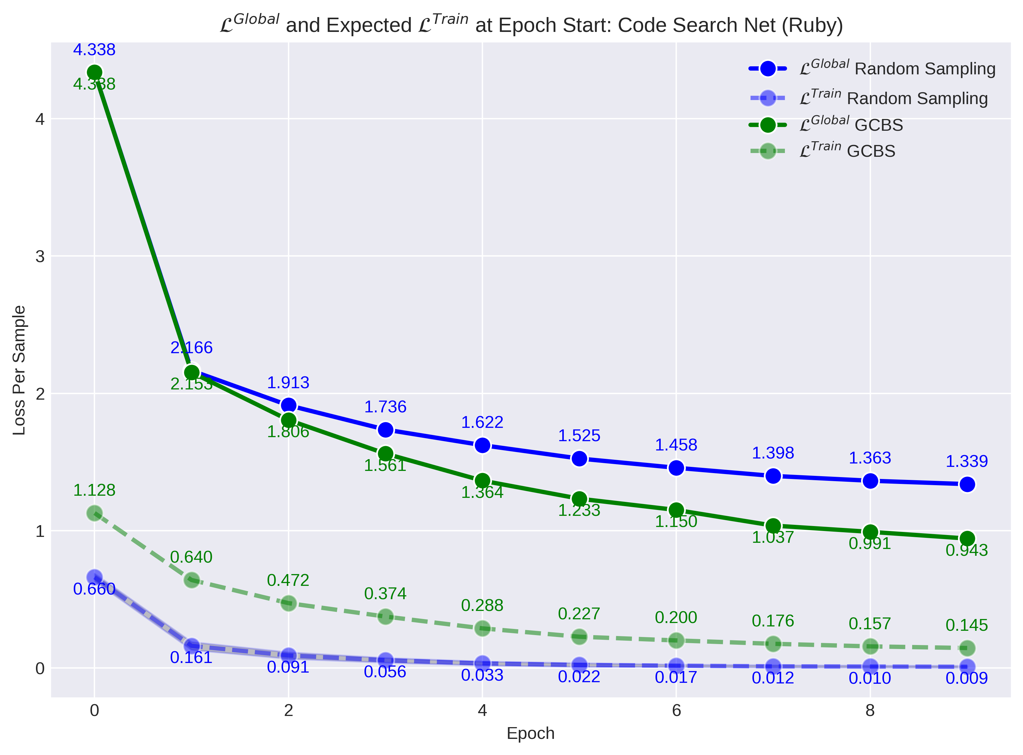
Figure 3: $\mathcal{L}^{Global}$ and Expected $\mathcal{L}^{Train}$ at the start of each epoch for Random Sampling and GCBS on the Code Search Net (Ruby) dataset with the UniXcoder model.

Empirically, we verify our theoretical contributions that Matrix Bandwidth Minimization will reduce the gap between $\mathcal{L}^{Global}-\mathcal{L}^{Train}$. To perform this study, we calculate the loss for in-batch negatives and the loss over all negatives for each sample when using either Random Sampling and GCBS for the Code Search Net (Ruby) dataset with the UniXcoder model. As shown in Figure 3, we find that using GCBS reduces the gap $\mathcal{L}^{Global}-\mathcal{L}^{Train}$ by  40% when compared to Random Sampling on the final epoch. Additionally, the total loss over all samples is reduced by 30% and, as shown in Appendix Section C, yields stronger validation/test performance.

8 Conclusion

In this paper, we introduced Global Contrastive Batch Sampling (GCBS), an efficient algorithm for better approximating global losses in contrastive learning through global batch assignments. GCBS is an approximation for quadratic assignment problems we prove characterize upper bounds for the gap between global and training losses in contrastive learning. Unlike previous approaches using hard negative mining, GCBS does not increase the training length of epochs by oversampling and is more efficient compared the most minimal hard negative mining approaches. We evaluate GCBS on sentence embedding and code search tasks and achieve state-of-the-art performance in both settings. Our method provides an efficient alternative to hard negative mining that is simple to implement, does not maintain additional data structures during training, provides strong performance, and performs global batch assignments.

Appendix A Derivation of Proofs for Theorems 4.1 and 4.2

In this section, we provide proof derivations of Theorems 4.1 and 4.2.

A.1 Proof of Theorem 4.1

We show that the formulation of the gap between the Global and Training contrastive losses $\mathcal{L}^{Global}-\mathcal{L}^{Train}$ when using the translation identity lower bound for Log-Sum-Exp (Nielsen & Sun, 2016) is approximated as a Quadratic Bottleneck Assignment Problem (QBAP). This optimization problem is associated with the lower bound in Theorem 3.6.

Since this formulation is not equivalent over $X$ and $Y$, we will first denote $\mathcal{L}^{Global}-\mathcal{L}^{Train}_{X}$ and $\mathcal{L}^{Global}-\mathcal{L}^{Train}_{Y}$ as the respective gaps over $X$ and $Y$ when using the translation identity lower bound on $\mathcal{L}^{Train}_{X},\mathcal{L}^{Train}_{Y}$:

$$\mathcal{L}^{Global}_{X}-\mathcal{L}^{Train}_{X}\leq \frac{1}{N}\sum_{i=1}^{N}{\tau}^{-1}(\max_{j}x_{i}^{T}y_{j}-\min_{j\in B_{i}}x_{i}^{T}y_{j})+\log\frac{N}{k}$$

$$\mathcal{L}^{Global}_{Y}-\mathcal{L}^{Train}_{Y}\leq \frac{1}{N}\sum_{i=1}^{N}{\tau}^{-1}(\max_{j}y_{i}^{T}x_{j}-\min_{j\in B_{i}}y_{i}^{T}x_{j})+\log\frac{N}{k}$$

Then we will minimize the optimization problem $\min_{B}\mathcal{L}^{Global}_{X}+\mathcal{L}^{Global}_{Y}-\mathcal{L}^{Train}_{X}-\mathcal{L}^{Train}_{Y}$ in order to equally weigh the selection of informative samples for both $X$ and $Y$. Lastly, denote $Z_{ij}\triangleq\min\{x_{i}^{T}y_{j},y_{i}^{T}x_{j}\}$ and $\odot$ as the Hadamard product.

Proof.

To formulate $\min_{B}\mathcal{L}^{Global}_{X}+\mathcal{L}^{Global}_{Y}-\mathcal{L}^{Train}_{X}-\mathcal{L}^{Train}_{Y}$ with the translation identity lower bound for Log-Sum-Exp as a QBAP, we need only use the fact that $\sum_{i}^{N}x_{i}\geq N\min_{i}x_{i}$.

$$\arg\min_{B}\mathcal{L}^{Global}_{X}+\mathcal{L}^{Global}_{Y}-\mathcal{L}^{Train}_{X}-\mathcal{L}^{Train}_{Y}= \arg\max_{B}\sum_{i=1}^{N}\min_{j\in B_{i}}x_{i}^{T}y_{j}+\min_{j\in B_{i}}y_{i}^{T}x_{j}$$ (1)

$$\geq 2\arg\max_{B}\sum_{i=1}^{N}\min\{\min_{j\in B_{i}}x_{i}^{T}y_{j},\min_{j\in B_{i}}y_{i}^{T}x_{j}\}$$

$$= 2\arg\max_{B}\sum_{i=1}^{N}\min_{j\in B_{i}}Z_{ij}$$

$$\geq 2N\arg\max_{B}\min_{i,j\in B}Z_{ij}$$

$$= 2N\arg\min_{\pi\in\Pi_{N}}\max_{i,j}-A\odot\pi Z\pi^{T}.$$

∎

A.2 Proof of Theorem 4.2

We show that the formulation of the gap between the Global and Training contrastive losses $\mathcal{L}^{Global}-\mathcal{L}^{Train}$ when using the standard lower bound for Log-Sum-Exp (Calafiore & El Ghaoui, 2014) is approximated as a Quadratic Assignment Problem (QAP). This optimization problem is associated with the lower bound Theorem 3.7.

Since this formulation is not equivalent over $X$ and $Y$, we will first denote $\mathcal{L}^{Global}-\mathcal{L}^{Train}_{X}$ and $\mathcal{L}^{Global}-\mathcal{L}^{Train}_{Y}$ as the respective gaps over $X$ and $Y$ when using the standard lower bound on $\mathcal{L}^{Train}_{X},\mathcal{L}^{Train}_{Y}$:

$$\mathcal{L}^{Global}_{X}-\mathcal{L}^{Train}_{X}\leq \frac{1}{N}\sum_{i=1}^{N}{\tau}^{-1}(\max_{j}x_{i}^{T}y_{j}-\max_{j\in B_{i}}x_{i}^{T}y_{j})+\log N$$

$$\mathcal{L}^{Global}_{Y}-\mathcal{L}^{Train}_{Y}\leq \frac{1}{N}\sum_{i=1}^{N}{\tau}^{-1}(\max_{j}y_{i}^{T}x_{j}-\max_{j\in B_{i}}y_{i}^{T}x_{j})+\log N$$

Then we will minimize the optimization problem $\min_{B}\mathcal{L}^{Global}_{X}+\mathcal{L}^{Global}_{Y}-\mathcal{L}^{Train}_{X}-\mathcal{L}^{Train}_{Y}$ in order to equally weigh the selection of informative samples for both $X$ and $Y$. Lastly, denote $\odot$ as the Hadamard product.

Proof.

To formulate $\min_{B}\mathcal{L}^{Global}_{X}+\mathcal{L}^{Global}_{Y}-\mathcal{L}^{Train}_{X}-\mathcal{L}^{Train}_{Y}$ as a QAP, we need only use the fact that $\max_{\{i\in 1,2,\dots,k\}}x_{i}\geq\frac{1}{k}\sum_{i}^{k}x_{i}$.

$$\arg\min_{B}\mathcal{L}^{Global}_{X}+\mathcal{L}^{Global}_{Y}-\mathcal{L}^{Train}_{X}-\mathcal{L}^{Train}_{Y}= \arg\max_{B}\sum_{i=1}^{N}\max_{j\in B_{i}}x_{i}^{T}y_{j}+\max_{j\in B_{i}}y_{i}^{T}x_{j}$$ (2)

$$\geq \frac{1}{k}\arg\max_{B}\sum_{i=1}^{N}\sum_{j\in B_{i}}x_{i}^{T}y_{j}+\frac{1}{k}\max_{B}\sum_{i=1}^{N}\sum_{j\in B_{i}}y_{i}^{T}x_{j}$$

$$= \frac{1}{k}\arg\max_{\pi\in\Pi_{N}}Tr(A\pi XY^{T}\pi^{T})+Tr((A\pi XY^{T}\pi^{T})^{T})$$

$$= \frac{1}{k}\arg\max_{\pi\in\Pi_{N}}Tr(A\pi(XY^{T}+YX^{T})\pi^{T}).$$

∎

Appendix B Expected loss values at Epoch Start for Random Sampling (10000 trials) in Code Search Net (Ruby)

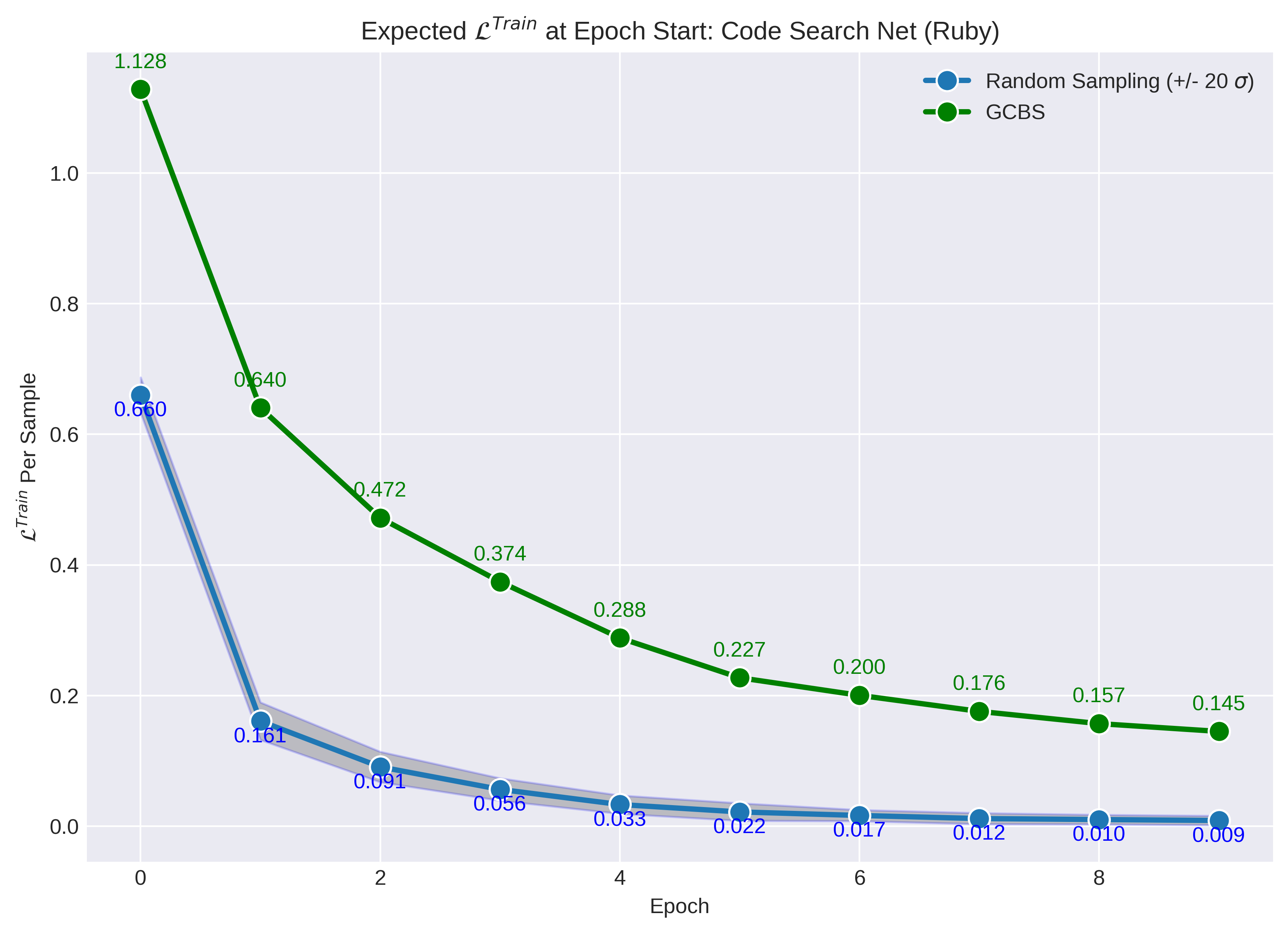
Figure 4: Expected $\mathcal{L}^{Train}$ for Random Sampling ($\pm 20\sigma$) and GCBS on the Code Search Net (Ruby) dataset with the UniXcoder model.

We calculate the expected loss for Random Sampling over 10,000 random batch assignments and compare these loss values to GCBS. The expected loss values for Random Sampling is clearly differentiated from Global Contrastive Batch Sampling even when compared with the mean over the 10,000 assignments plus $20$ standard deviations as shown in Figure 4. As a result, the loss incurred by GCBS is a better proxy of the global loss even compared to the largest loss incurred among 10,000 random assignments. Empirically, this shows that GCBS provides improvements in Global batch assignment that are unlikely to be obtained by selecting across random assignments.

Appendix C Validation Performance comparison for GCBS, Random Sampling, and Hard Negative Mining

In this section, we provide validation and test performance for GCBS, Random Sampling, and Hard Negative Mining for the Code Search Net (Ruby) dataset with the UniXcoder model. We find that GCBS provides validation and test performance improvements compared to both Random Sampling and Hard Negative (1). In particular, the gap between test performance for GCBS and Hard Negative (1) is greater than that of Hard Negative (1) and Random Sampling.

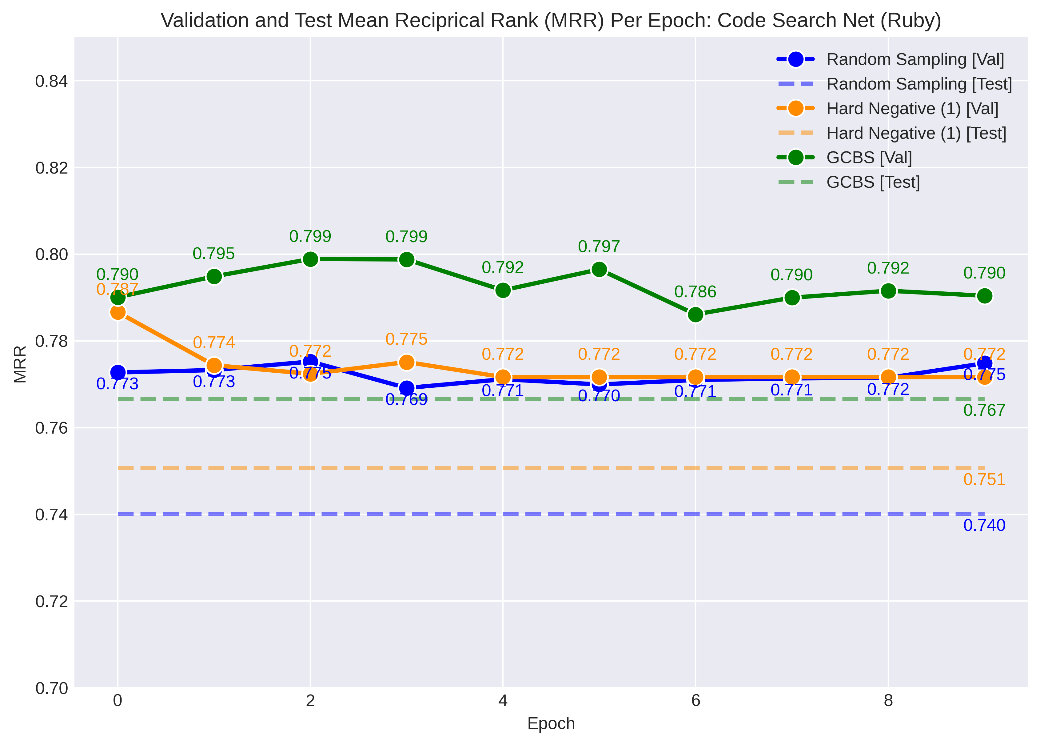
Figure 5: Validation and Test Performance for Random Sampling, Hard Negative (1), and GCBS on the Code Search Net (Ruby) dataset with the UniXcoder model (Guo et al., 2022).

Appendix D Expected positive class Softmax probability at epoch start for GCBS, Random Sampling, and Global

In this section, we provide the expected softmax probability at the start of each epoch across in-batch negatives when using GCBS and Random Sampling and across all negative samples (i.e. Global setting) for the Code Search Net (Ruby) task with the UniXcoder model. We find that GCBS better approximates the softmax probability of positive classes compared to random sampling and that random sampling results in loss saturation within a small number of epochs.

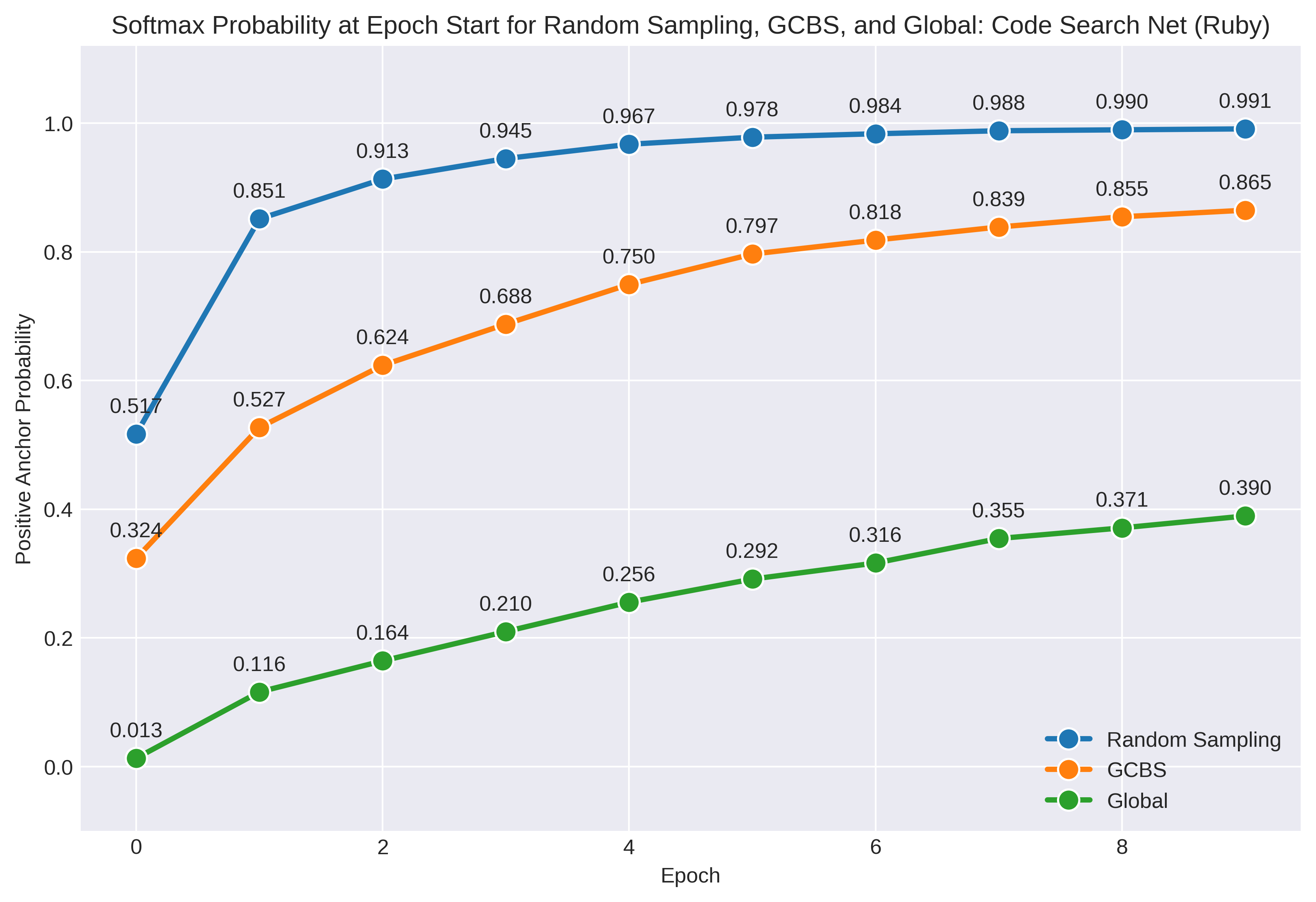
Figure 6: Expected positive anchor Softmax Probability for Code Search Net (Ruby) task using the UniXcoder model (Guo et al., 2022).

Appendix E Complexity Analysis of Global Contrastive Batch Sampling

E.1 Quantile Estimation

First, it is necessary to compute the value at the quantile $q$ in order to sparsify $XY^{T}$. For large datasets in our experiments, this operation is estimated over chunks of $XY^{T}$ and the median quantile value over the chunks is used. For each chunk of size $l$, this requires computing values of $XY^{T}$, performing a sort on these values and getting the index of the sorted values for the specified quantile. We denote matrix multiplication time complexity between two matrices as $MM(\cdot,\cdot)$ and show that this estimation has time complexity approximately equivalent to the matrix multiplication $XY^{T}$. We make the assumption that $d\geq\log(Nl)$.

$$\text{Space Complexity}= \underbrace{Nl^{-1}}_{\text{Chunk quantile values}}+\underbrace{Nl}_{\text{items in each chunk}}=\mathcal{O}(Nl)$$ (3)

$$\text{Time Complexity}= 2Nl^{-1}(\underbrace{\mathcal{O}(Nl\log(Nl))}_{\begin{subarray}{c}\text{Sort inner products}\end{subarray}}+\underbrace{MM(Nd,ld)}_{\text{Calculate inner products}})=\mathcal{O}(N^{2}d)$$

E.2 Optimizing over row permutations of X, Y

After estimating a value at which to sparsify, we need to get a sparsified similarity matrix $\tilde{XY}^{T}$, construct a sparse adjacency matrix and run the Cuthill McKee algorithm. We assume that $N(1-q)$, or the expected number of entries in each row is a small multiple of the batch size $k$. First, we detail the space and time complexity for constructing $\tilde{XY}^{T}$:

$$\text{Space Complexity}= \underbrace{3N^{2}(1-q)}_{\text{Row, Column, and Data values of $\tilde{XY}^{T}$}}=\mathcal{O}(Nk)$$ (4)

$$\text{Time Complexity}= \underbrace{Nl^{-1}MM(Nd,ld)}_{\text{Calculate inner products and threshold}}=\mathcal{O}(N^{2}d)$$

The space and time complexity for running the Cuthill McKee algorithm on $\tilde{XY}^{T}$ is detailed below, we assume the implementation from (Chan & George, 1980) is used which provides runtime bounded by $N^{2}$ up to logarithmic factors.

$$\text{Space Complexity}= \underbrace{3N^{2}(1-q)}_{\text{Row, Column, and Data values of $\tilde{XY}^{T}$}}=\mathcal{O}(Nk)$$ (5)

$$\text{Time Complexity}= \underbrace{\mathcal{O}(mN\log(m))}_{\text{Cuthill-Mckee Runtime}}\leq\underbrace{\mathcal{O}(N^{2}\log(N))}_{\text{Worst case, $m=N$}}$$

Note that $m$ is the maximum degree over nodes and for a large quantile value will typically be smaller than $N$. We find that Global Contrastive Batch Sampling incurs $\mathcal{O}(Nk)$ space complexity and $\mathcal{O}(N^{2}d)$ time complexity.

Appendix F Implementation in PyTorch

In this section, we detail efficient implementation of GCBS in PyTorch. Our implementation computes a permutation over samples $\pi$ at the beginning of each epoch, requires less than 50 lines of code, makes no changes to the model being trained, and does not maintain external data structures after being run between epochs.

The PyTorch pseudocode for the implementation of GCBS is contained below. In the case where $XY^{T}$ cannot be held in memory, the value of the quantile $q$ can be approximated over subsamples of entries from $XY^{T}$ and the sparse matrix $\tilde{XY}^{T}$ can be constructed similarly.

⬇

def compute_perm_bandwidth_min(X, Y, quantile_thresh = 0.999):

# (1) Normalize representations.

X, Y = normalize(X), normalize(Y)

# (2) Get value at quantile threshold on the inner product matrix.

quantile_thresh = torch.quantile(X @ Y.T, quantile_thresh)

# (3) Get inner product matrix hard thresholded on quantile.

row, col, data = [], [], []

# Get rows and columns of indices > estimated quantile value

ret = ((X @ Y.T).flatten() > quantile_thresh).nonzero

row += ((ret - (ret % num_samples))/num_samples).tolist()

col += (ret % num_samples).tolist()

data += [1.0 for _ in range(len(ret))]

# (4) Get perm which minimizes bandwidth of sparsified matrix with Cuthill-McKee.

permutation = list(cuthill_mckee(sparse_matrix((data, (row, col)),

shape=(num_samples, num_samples))))

return permutation

In the next code block, we provide PyTorch pseudocode which, when inserted at the beginning of each epoch, will call the previous method and apply the permutation over samples before training. Note that the SequentialSampler is utilized to control batches after samples are reordered.

⬇

## (1) At epoch start, run forward pass to get representations X, Y in the paired dataset.

model.eval()

with torch.no_grad():

X, Y = [], []

for batch in train_dataloader:

X.append(model(inputs=batch[0]))

Y.append(model(inputs=batch[1]))

## (2) Compute an approx to permutation which minimizes bandwidth of \pi XY^T \pi^T for entries greater than quantile q.

permutation = compute_perm_bandwidth_min(X, Y, quantile=q)

## (3) Reorder the dataset on the approximate solution.

train_dataset = torch.utils.data.Subset(train_dataset, permutation)

train_sampler = SequentialSampler(train_dataset)

train_dataloader = DataLoader(train_dataset,

sampler=train_sampler,

batch_size=train_batch_size)

model.train()

## (4) Continue training.

Appendix G Dataset Details

In Table 7 and Table 8, we provide details for all Sentence Embedding and Code Search datasets respectively.

Setting	Name	# of samples	Source
Train	SNLI+MNLI (entailment+hard neg)	275,602	Hugging Face Download
Test	STS12	3.1K	Hugging Face Download
Test	STS13	1.5K	Hugging Face Download
Test	STS14	3.7K	Hugging Face Download
Test	STS15	8.5K	Hugging Face Download
Test	STS16	9.2K	Hugging Face Download
Test	STS-B	1.4K	Hugging Face Download
Test	SICK-R	4.9K	Hugging Face Download

Table 7: Description of training and evaluation datasets for sentence embedding tasks, all datasets are from (Gao et al., 2021) and further details can be found in the repository.

Name	Train samples	Validation	Test Samples	# of Candidates	Source
CosQA	20,000	604	1,046	1,046	CodeBERT Repo
AdvTest	251,820	9,604	19,210	19,210	CodeBERT Repo
CSN Go	167,288	7,325	8,122	28,120	CodeBERT Repo
CSN Java	164,923	5,183	10,955	40,347	CodeBERT Repo
CSN JavaScript	58,025	3,885	3,291	13,981	CodeBERT Repo
CSN PHP	241,241	12,982	14,014	52,660	CodeBERT Repo
CSN Python	251,820	13,914	14,918	43,827	CodeBERT Repo
CSN Ruby	24,927	1,400	1,261	4,360	CodeBERT Repo

Table 8: Description of training and evaluation datasets for code search tasks, all datasets are from (Feng et al., 2020) and further details can be found in the repository.

Appendix H Hyperparameters

In Tables 9 and 10 below, we detail the hyperparameters used for the best performing sentence embedding and code search models respectively.

Model	Learning Rate	Batch Size	Number Epochs	Quantile $q$
SimCSE BERTbase	$3e{-5}$	256	5	0.999
SimCSE RoBERTabase	$3e{-5}$	256	5	0.999
SimCSE RoBERTalarge	$7e{-6}$	256	5	0.9999
PromCSE BERTbase	$7e{-3}$	256	10	0.999
PromCSE RoBERTabase	$7e{-3}$	256	10	0.999
PromCSE RoBERTalarge	$7e{-3}$	256	10	0.999

Table 9: Hyperparameters for best experimental results in Sentence Embedding tasks.

Task	Learning Rate	Batch Size	Number Epochs	Quantile $q$
CosQA	$2e{-5}$	64	10	0.999
AdvTest	$2e{-5}$	64	10	0.999
CSN Ruby	$2e{-5}$	64	10	0.999
CSN Go	$2e{-5}$	64	10	0.999
CSN JS	$2e{-5}$	64	10	0.999
CSN Python	$2e{-5}$	64	10	0.999
CSN Java	$2e{-5}$	64	10	0.999
CSN PHP	$2e{-5}$	64	10	0.999

Table 10: Hyperparameters for best experimental results in Code Search tasks for the UniXcoder model.

For Sentence Embedding tasks, hyperparameters do not vary significantly, other than the learning rate, between models and are similar to those used in the original models with random sampling (Gao et al., 2021; Yuxin Jiang & Wang, 2022). For Code Search tasks, we do not vary hyperparameters from the default values from the original paper using random sampling (Guo et al., 2022) and, as a result, we use identical settings to the UniXcoder paper other than batch assignments.

Appendix I Comparison of batch loss values between GCBS, Random Sampling, and Hard Negative Mining

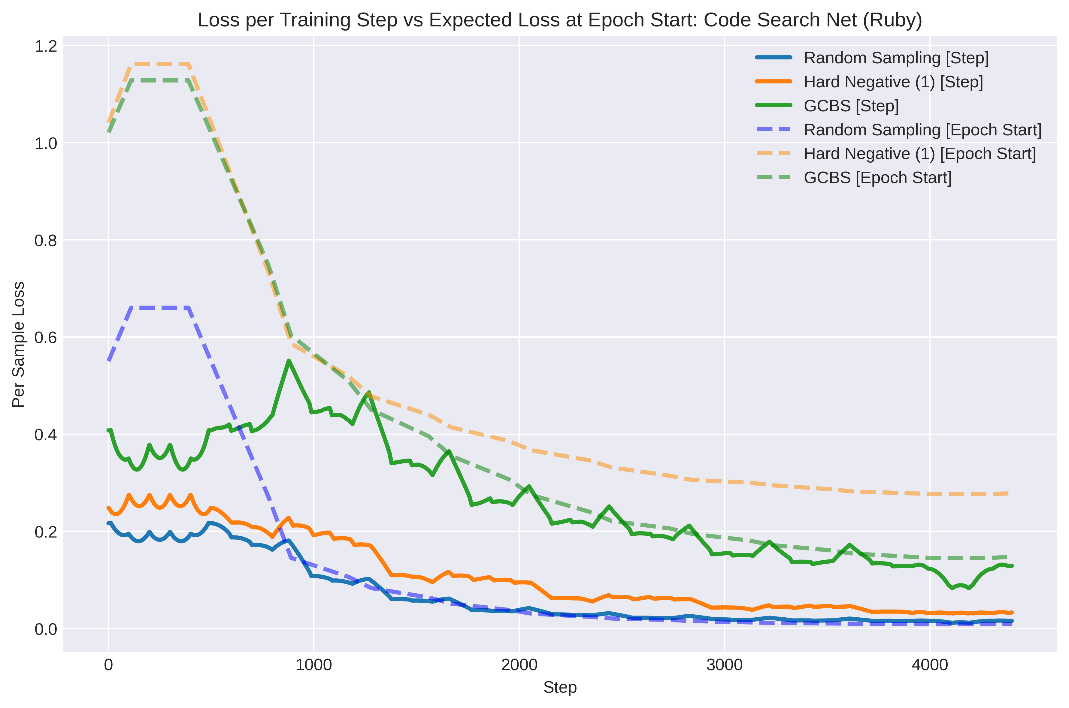
Figure 7: Loss per sample and expected loss computed at epoch start for GCBS, Random Sampling, and Hard Negative (1) for the Code Search Net (Ruby) dataset with the UniXcoder model.

In Figure 7, we show the loss per sample vs step number in the Code Search Net (Ruby) dataset with the UniXCoder model for Random Sampling, GCBS, and mining $1$ hard negative per sample at the beginning of each epoch which we denote as Hard Negative (1). This hard mining approach has a smaller computational burden compared with approaches commonly used in practice but incurs 2x the runtime of GCBS and 3x the runtime of random sampling as detailed in Section 7.1.

Additionally, we compare each training step loss to the expected loss over batches calculated at the beginning of each epoch. This requires performing a forward pass at the start of each epoch, assigning batches, and then computing the loss over in-batch negatives for each sample. After the first few epochs, while the expected loss over batches for Random Sampling and GCBS is well approximated by the expected loss at the epoch start, expected losses for Hard Negative Mining are substantially overestimated. This corroborates findings in previous literature (Wang et al., 2021; Xiong et al., 2021) which motivates the need to update nearest neighbor indices frequently within an epoch, further increasing the computational burden of Hard Negative Mining. Empirically, we find that the observed loss per sample for GCBS is significantly larger than that of Random Sampling or Hard Negative (1) and, like Random Sampling but not Hard Negative (1), can be well approximated by the expected loss at the epoch start. Losses are smoothed as a running average over the previous $500$ training steps.

Appendix J Runtime scaling of GCBS vs number of samples $N$

In order to empirically characterize the runtime scaling of GCBS with respect to the number of samples $N$, we run simulations with random embeddings of dimension 768 both in 1 GPU and 7 GPU settings. Results for these experiments are included in Table 12 and Table 12. For all experimentation, we scale the quantile value to keep 512 expected values in each row/column after sparsification (i.e. $q=1-\frac{512}{N}$).

N	Runtime (seconds)
10000	2.56
50000	14.77
100000	34.68
500000	322.52
1000000	1013.19

Table 11: Runtime scaling of GCBS on a single A40 GPU with respect to number of samples $N$

N	Runtime (seconds)
10000	31.05
50000	38.17
100000	52.85
500000	241.91
1000000	591.55
5000000	3956.39

Table 12: Runtime scaling of GCBS on 7 A40 GPUs with respect to number of samples $N$

We find that on a single A40 GPU, $N=10^{6}$ is tractable in under 20 minutes and for 7 GPUs $N=5\times 10^{6}$ is tractable in under 1 hour. We believe for very large scale datasets, initial space partitioning with a nearest neighbors library (i.e. FAISS) and then using our approach on partitions of size $10^{6}$ may be beneficial. An exact implementation of profiled code in these experiments for 1 GPU experiments are provided below.

⬇

import torch

import timeit

import math

from scipy.sparse.csgraph import reverse_cuthill_mckee

from scipy.sparse import csr_matrix

import statistics

def compute_gcbs(z1_outs, z2_outs, quantile):

start_time = timeit.default_timer()

# (1) Stack and normalize outputs

src_train_full = torch.nn.functional.normalize(z1_outs).cuda()

tgt_train_full = torch.nn.functional.normalize(z2_outs).cuda()

z1_outs, z2_outs = [], []

# (2) Estimate quantile

chunk_size, num_samples, quantiles = 3, len(tgt_train_full), []

for chunk_idx in range(math.ceil(len(tgt_train_full)/chunk_size)):

mat_val = src_train_full[chunk_idx*chunk_size:(chunk_idx+1)*chunk_size] @ tgt_train_full.T

quantiles.append(float(torch.quantile(mat_val, quantile)))

# (3) Get similarity graph thresholded on quantile

row, col, data, quantile = [], [], [], statistics.median(quantiles)

for chunk_idx in range(math.ceil(len(src_train_full)/chunk_size)):

mat_val = src_train_full[chunk_idx*chunk_size:(chunk_idx+1)*chunk_size] @ tgt_train_full.T

ret = (mat_val.flatten() > quantile).nonzero(as_tuple=True)[0].cpu()

row += ((ret - (ret % num_samples))/num_samples + chunk_idx*chunk_size).int().tolist()

col += (ret % num_samples).tolist()

data += [1.0 for _ in range(len(ret))]

# (4) Get permutation using graph bandwidth minimization on sparsified graph (cuthill-mckee)

permutation = list(reverse_cuthill_mckee(csr_matrix((data, (row, col)),

shape=(num_samples, num_samples))))

print(timeit.default_timer() - start_time)

return permutation

for size in [10000, 50000, 100000, 500000, 1000000]:

keep_per_sample = 512

z1, z2 = torch.rand(size, 768), torch.rand(size, 768)

quantile = 1 - float(keep_per_sample/size)

perm = compute_gcbs(z1, z2, quantile)

Appendix K Variation in Performance across Random Seeds

Since our proposed method GCBS is a deterministic algorithm, the only randomness in performance is from the parameter initialization of the pooling layer. We conduct 5 runs of the experiments with different seeds. The standard deviations on sentence embedding tasks with BERT base are:

Model	STS12	STS13	STS14	STS15	STS16	STS-B	SICK-R	Avg
SimCSE BERTbase w/ GCBS	75.82 $\pm$ 0.06	85.30 $\pm$ 0.02	81.12 $\pm$ 0.17	86.58 $\pm$ 0.11	81.68 $\pm$ 0.05	84.80 $\pm$ 0.01	80.04 $\pm$ 0.05	82.19 $\pm$ 0.05

Table 13: The performance and standard deviations across seeds for SimCSE BERT_base (Gao et al., 2021) with GCBS. The reported score is Spearman correlation magnified by a factor of 100.

The standard deviation on the CosQA code search task with the UniXcoder model are:

Model	CosQA
UniXcoder w/ GCBS	71.1 $\pm$ 0.26

Table 14: The performance and standard deviations across seeds for the UniXcoder (Guo et al., 2022) model with GCBS. The reported score is Mean Reciprical Rank magnified by a factor of 100.

The standard deviation of GCBS’s average performance on sentence embedding tasks is 0.05%, while the the relative performance is 0.62%. The standard deviation of GCBS’s performance on CosQA is 0.26%, while the relative improvement is 1.0%.

Appendix L Limitations

Our GCBS approach, while efficient compared to alternatives, does increase the runtime of standard contrastive learning approaches (i.e. SimCLR, Moco). As a result, it increases training costs for experiments which would be limiting for some researchers. In large scale settings (i.e. $>5\times 10^{6}$ paired samples), additional steps to partition the training data for parallel processing may be required before using our approach.

References

- Burkard (1984) Burkard, R. E. Quadratic assignment problems. European Journal of Operational Research, 15(3):283–289, 1984. ISSN 0377-2217. doi: https://doi.org/10.1016/0377-2217(84)90093-6. URL https://www.sciencedirect.com/science/article/pii/0377221784900936.
- Calafiore & El Ghaoui (2014) Calafiore, G. and El Ghaoui, L. Optimization Models. Control systems and optimization series. Cambridge University Press, October 2014.
- Chan & George (1980) Chan, W. M. and George, A. A linear time implementation of the reverse cuthill-mckee algorithm. BIT, 20(1):8–14, mar 1980. ISSN 0006-3835. doi: 10.1007/BF01933580. URL https://doi.org/10.1007/BF01933580.
- Chen et al. (2020a) Chen, T., Kornblith, S., Norouzi, M., and Hinton, G. A simple framework for contrastive learning of visual representations. In III, H. D. and Singh, A. (eds.), Proceedings of the 37th International Conference on Machine Learning, volume 119 of Proceedings of Machine Learning Research, pp. 1597–1607. PMLR, 13–18 Jul 2020a. URL https://proceedings.mlr.press/v119/chen20j.html.
- Chen et al. (2020b) Chen, X., Fan, H., Girshick, R. B., and He, K. Improved baselines with momentum contrastive learning. CoRR, abs/2003.04297, 2020b. URL https://arxiv.org/abs/2003.04297.
- Chuang et al. (2020) Chuang, C.-Y., Robinson, J., Lin, Y.-C., Torralba, A., and Jegelka, S. Debiased contrastive learning. In Larochelle, H., Ranzato, M., Hadsell, R., Balcan, M., and Lin, H. (eds.), Advances in Neural Information Processing Systems, volume 33, pp. 8765–8775. Curran Associates, Inc., 2020. URL https://proceedings.neurips.cc/paper/2020/file/63c3ddcc7b23daa1e42dc41f9a44a873-Paper.pdf.
- Cuthill & McKee (1969) Cuthill, E. and McKee, J. Reducing the bandwidth of sparse symmetric matrices. In Proceedings of the 1969 24th National Conference, ACM ’69, pp. 157–172, New York, NY, USA, 1969. Association for Computing Machinery. ISBN 9781450374934. doi: 10.1145/800195.805928. URL https://doi.org/10.1145/800195.805928.
- Edmonds & Karp (1972) Edmonds, J. and Karp, R. M. Theoretical improvements in algorithmic efficiency for network flow problems. J. ACM, 19(2):248–264, apr 1972. ISSN 0004-5411. doi: 10.1145/321694.321699. URL https://doi.org/10.1145/321694.321699.
- Feige (2000) Feige, U. Coping with the np-hardness of the graph bandwidth problem. In Algorithm Theory - SWAT 2000, pp. 10–19, Berlin, Heidelberg, 2000. Springer Berlin Heidelberg. ISBN 978-3-540-44985-0.
- Feng et al. (2020) Feng, Z., Guo, D., Tang, D., Duan, N., Feng, X., Gong, M., Shou, L., Qin, B., Liu, T., Jiang, D., and Zhou, M. CodeBERT: A pre-trained model for programming and natural languages. In Findings of the Association for Computational Linguistics: EMNLP 2020, pp. 1536–1547, Online, November 2020. Association for Computational Linguistics. doi: 10.18653/v1/2020.findings-emnlp.139. URL https://aclanthology.org/2020.findings-emnlp.139.
- Gao et al. (2021) Gao, T., Yao, X., and Chen, D. SimCSE: Simple contrastive learning of sentence embeddings. In Empirical Methods in Natural Language Processing (EMNLP), 2021.
- Ge et al. (2018) Ge, W., Huang, W., Dong, D., and Scott, M. R. Deep metric learning with hierarchical triplet loss. In ECCV, 2018.
- Guo et al. (2021) Guo, D., Ren, S., Lu, S., Feng, Z., Tang, D., LIU, S., Zhou, L., Duan, N., Svyatkovskiy, A., Fu, S., Tufano, M., Deng, S. K., Clement, C., Drain, D., Sundaresan, N., Yin, J., Jiang, D., and Zhou, M. Graphcode{bert}: Pre-training code representations with data flow. In International Conference on Learning Representations, 2021. URL https://openreview.net/forum?id=jLoC4ez43PZ.
- Guo et al. (2022) Guo, D., Lu, S., Duan, N., Wang, Y., Zhou, M., and Yin, J. UniXcoder: Unified cross-modal pre-training for code representation. In Proceedings of the 60th Annual Meeting of the Association for Computational Linguistics (Volume 1: Long Papers), pp. 7212–7225, Dublin, Ireland, May 2022. Association for Computational Linguistics. doi: 10.18653/v1/2022.acl-long.499. URL https://aclanthology.org/2022.acl-long.499.
- Harwood et al. (2017) Harwood, B., Kumar B.G., V., Carneiro, G., Reid, I., and Drummond, T. Smart mining for deep metric learning. In 2017 IEEE International Conference on Computer Vision (ICCV), pp. 2840–2848, 2017. doi: 10.1109/ICCV.2017.307.
- He et al. (2020) He, K., Fan, H., Wu, Y., Xie, S., and Girshick, R. Momentum contrast for unsupervised visual representation learning. In 2020 IEEE/CVF Conference on Computer Vision and Pattern Recognition (CVPR), pp. 9726–9735, 2020. doi: 10.1109/CVPR42600.2020.00975.
- Ho & Nvasconcelos (2020) Ho, C.-H. and Nvasconcelos, N. Contrastive learning with adversarial examples. In Larochelle, H., Ranzato, M., Hadsell, R., Balcan, M., and Lin, H. (eds.), Advances in Neural Information Processing Systems, volume 33, pp. 17081–17093. Curran Associates, Inc., 2020. URL https://proceedings.neurips.cc/paper/2020/file/c68c9c8258ea7d85472dd6fd0015f047-Paper.pdf.
- Husain et al. (2019) Husain, H., Wu, H.-H., Gazit, T., Allamanis, M., and Brockschmidt, M. CodeSearchNet challenge: Evaluating the state of semantic code search. arXiv preprint arXiv:1909.09436, 2019.
- Iscen et al. (2018) Iscen, A., Tolias, G., Avrithis, Y., and Chum, O. Mining on Manifolds: Metric Learning without Labels. In CVPR 2018 - IEEE Computer Vision and Pattern Recognition Conference, pp. 1–10, Salt Lake City, United States, June 2018. IEEE. URL https://hal.inria.fr/hal-01843085.
- Jonker & Volgenant (1988) Jonker, R. and Volgenant, T. A shortest augmenting path algorithm for dense and sparse linear assignment problems. In Schellhaas, H., van Beek, P., Isermann, H., Schmidt, R., and Zijlstra, M. (eds.), DGOR/NSOR, pp. 622–622, Berlin, Heidelberg, 1988. Springer Berlin Heidelberg. ISBN 978-3-642-73778-7.
- Kalantidis et al. (2020) Kalantidis, Y., Sariyildiz, M. B., Pion, N., Weinzaepfel, P., and Larlus, D. Hard negative mixing for contrastive learning. In Larochelle, H., Ranzato, M., Hadsell, R., Balcan, M., and Lin, H. (eds.), Advances in Neural Information Processing Systems, volume 33, pp. 21798–21809. Curran Associates, Inc., 2020. URL https://proceedings.neurips.cc/paper/2020/file/f7cade80b7cc92b991cf4d2806d6bd78-Paper.pdf.
- Khosla et al. (2020) Khosla, P., Teterwak, P., Wang, C., Sarna, A., Tian, Y., Isola, P., Maschinot, A., Liu, C., and Krishnan, D. Supervised contrastive learning. In Larochelle, H., Ranzato, M., Hadsell, R., Balcan, M., and Lin, H. (eds.), Advances in Neural Information Processing Systems, volume 33, pp. 18661–18673. Curran Associates, Inc., 2020. URL https://proceedings.neurips.cc/paper/2020/file/d89a66c7c80a29b1bdbab0f2a1a94af8-Paper.pdf.
- Kim et al. (2020) Kim, M., Tack, J., and Hwang, S. J. Adversarial self-supervised contrastive learning. In Larochelle, H., Ranzato, M., Hadsell, R., Balcan, M., and Lin, H. (eds.), Advances in Neural Information Processing Systems, volume 33, pp. 2983–2994. Curran Associates, Inc., 2020. URL https://proceedings.neurips.cc/paper/2020/file/1f1baa5b8edac74eb4eaa329f14a0361-Paper.pdf.
- Koopmans & Beckmann (1957) Koopmans, T. C. and Beckmann, M. Assignment problems and the location of economic activities. Econometrica, 25(1):53–76, 1957. ISSN 00129682, 14680262. URL http://www.jstor.org/stable/1907742.
- Kuhn (1955) Kuhn, H. W. The hungarian method for the assignment problem. Naval Research Logistics Quarterly, 2(1-2):83–97, 1955. doi: https://doi.org/10.1002/nav.3800020109. URL https://onlinelibrary.wiley.com/doi/abs/10.1002/nav.3800020109.
- Laskin et al. (2020) Laskin, M., Srinivas, A., and Abbeel, P. Curl: Contrastive unsupervised representations for reinforcement learning. Proceedings of the 37th International Conference on Machine Learning, Vienna, Austria, PMLR 119, 2020. arXiv:2004.04136.
- Logeswaran & Lee (2018) Logeswaran, L. and Lee, H. An efficient framework for learning sentence representations. In International Conference on Learning Representations, 2018. URL https://openreview.net/forum?id=rJvJXZb0W.
- Mishchuk et al. (2017) Mishchuk, A., Mishkin, D., Radenović, F., and Matas, J. Working hard to know your neighbor’s margins: Local descriptor learning loss. In Proceedings of the 31st International Conference on Neural Information Processing Systems, NIPS’17, pp. 4829–4840, Red Hook, NY, USA, 2017. Curran Associates Inc. ISBN 9781510860964.
- Munkres (1957) Munkres, J. Algorithms for the assignment and transportation problems. Journal of the Society for Industrial and Applied Mathematics, 5(1):32–38, 1957. ISSN 03684245. URL http://www.jstor.org/stable/2098689.
- Nielsen & Sun (2016) Nielsen, F. and Sun, K. Guaranteed bounds on the kullback-leibler divergence of univariate mixtures using piecewise log-sum-exp inequalities. CoRR, abs/1606.05850, 2016. URL http://arxiv.org/abs/1606.05850.
- Radford et al. (2021) Radford, A., Kim, J. W., Hallacy, C., Ramesh, A., Goh, G., Agarwal, S., Sastry, G., Askell, A., Mishkin, P., Clark, J., Krueger, G., and Sutskever, I. Learning transferable visual models from natural language supervision. CoRR, abs/2103.00020, 2021. URL https://arxiv.org/abs/2103.00020.
- Ramesh et al. (2021) Ramesh, A., Pavlov, M., Goh, G., Gray, S., Voss, C., Radford, A., Chen, M., and Sutskever, I. Zero-shot text-to-image generation. CoRR, abs/2102.12092, 2021. URL https://arxiv.org/abs/2102.12092.
- Robinson et al. (2021) Robinson, J. D., Chuang, C.-Y., Sra, S., and Jegelka, S. Contrastive learning with hard negative samples. In International Conference on Learning Representations, 2021. URL https://openreview.net/forum?id=CR1XOQ0UTh-.
- Saeed et al. (2021) Saeed, A., Grangier, D., and Zeghidour, N. Contrastive learning of general-purpose audio representations. In ICASSP 2021 - 2021 IEEE International Conference on Acoustics, Speech and Signal Processing (ICASSP), pp. 3875–3879, 2021. doi: 10.1109/ICASSP39728.2021.9413528.
- Saunshi et al. (2019) Saunshi, N., Plevrakis, O., Arora, S., Khodak, M., and Khandeparkar, H. A theoretical analysis of contrastive unsupervised representation learning. In Chaudhuri, K. and Salakhutdinov, R. (eds.), Proceedings of the 36th International Conference on Machine Learning, volume 97 of Proceedings of Machine Learning Research, pp. 5628–5637. PMLR, 09–15 Jun 2019. URL https://proceedings.mlr.press/v97/saunshi19a.html.
- Schroff et al. (2015) Schroff, F., Kalenichenko, D., and Philbin, J. Facenet: A unified embedding for face recognition and clustering. In 2015 IEEE Conference on Computer Vision and Pattern Recognition (CVPR), pp. 815–823, 2015. doi: 10.1109/CVPR.2015.7298682.
- Sohn (2016) Sohn, K. Improved deep metric learning with multi-class n-pair loss objective. In Lee, D., Sugiyama, M., Luxburg, U., Guyon, I., and Garnett, R. (eds.), Advances in Neural Information Processing Systems, volume 29. Curran Associates, Inc., 2016. URL https://proceedings.neurips.cc/paper/2016/file/6b180037abbebea991d8b1232f8a8ca9-Paper.pdf.
- Song et al. (2016) Song, H. O., Xiang, Y., Jegelka, S., and Savarese, S. Deep metric learning via lifted structured feature embedding. In Computer Vision and Pattern Recognition (CVPR), 2016.
- Steinberg (1961) Steinberg, L. The backboard wiring problem: A placement algorithm. SIAM Review, 3(1):37–50, 1961. ISSN 00361445. URL http://www.jstor.org/stable/2027247.
- Sylvain et al. (2020) Sylvain, T., Petrini, L., and Hjelm, D. Locality and compositionality in zero-shot learning. In International Conference on Learning Representations, 2020. URL https://openreview.net/forum?id=Hye_V0NKwr.
- Wang et al. (2021) Wang, J., Zhu, J., and He, X. Cross-batch negative sampling for training two-tower recommenders. Proceedings of the 44th International ACM SIGIR Conference on Research and Development in Information Retrieval, 2021.
- Wu et al. (2017) Wu, C.-Y., Manmatha, R., Smola, A. J., and Krähenbühl, P. Sampling matters in deep embedding learning. In 2017 IEEE International Conference on Computer Vision (ICCV), pp. 2859–2867, 2017. doi: 10.1109/ICCV.2017.309.
- Xiong et al. (2021) Xiong, L., Xiong, C., Li, Y., Tang, K.-F., Liu, J., Bennett, P. N., Ahmed, J., and Overwijk, A. Approximate nearest neighbor negative contrastive learning for dense text retrieval. In International Conference on Learning Representations, 2021. URL https://openreview.net/forum?id=zeFrfgyZln.
- Xuan et al. (2020) Xuan, H., Stylianou, A., Liu, X., and Pless, R. Hard negative examples are hard, but useful. In ECCV, 2020.
- Yang et al. (2022) Yang, C., An, Z., Cai, L., and Xu, Y. Mutual contrastive learning for visual representation learning. Proceedings of the AAAI Conference on Artificial Intelligence, 36(3):3045–3053, Jun. 2022. doi: 10.1609/aaai.v36i3.20211. URL https://ojs.aaai.org/index.php/AAAI/article/view/20211.
- Yang et al. (2021) Yang, Z., Yang, Y., Cer, D., Law, J., and Darve, E. Universal sentence representation learning with conditional masked language model. In Proceedings of the 2021 Conference on Empirical Methods in Natural Language Processing, pp. 6216–6228, 2021.
- Yu et al. (2022) Yu, J., Wang, Z., Vasudevan, V., Yeung, L., Seyedhosseini, M., and Wu, Y. Coca: Contrastive captioners are image-text foundation models, 2022. URL https://arxiv.org/abs/2205.01917.
- Yuxin Jiang & Wang (2022) Yuxin Jiang, L. Z. and Wang, W. Improved universal sentence embeddings with prompt-based contrastive learning and energy-based learning, 2022.
- Zhang et al. (2018) Zhang, H., Cisse, M., Dauphin, Y. N., and Lopez-Paz, D. mixup: Beyond empirical risk minimization. In International Conference on Learning Representations, 2018. URL https://openreview.net/forum?id=r1Ddp1-Rb.
- Zhang & Stratos (2021) Zhang, W. and Stratos, K. Understanding hard negatives in noise contrastive estimation. In Proceedings of the 2021 Conference of the North American Chapter of the Association for Computational Linguistics: Human Language Technologies, pp. 1090–1101, Online, June 2021. Association for Computational Linguistics. doi: 10.18653/v1/2021.naacl-main.86. URL https://aclanthology.org/2021.naacl-main.86.