Optimal Discriminant Analysis in High-Dimensional Latent Factor Models
Abstract
In high-dimensional classification problems, a commonly used approach is to first project the high-dimensional features into a lower dimensional space, and base the classification on the resulting lower dimensional projections. In this paper, we formulate a latent-variable model with a hidden low-dimensional structure to justify this two-step procedure and to guide which projection to choose. We propose a computationally efficient classifier that takes certain principal components (PCs) of the observed features as projections, with the number of retained PCs selected in a data-driven way. A general theory is established for analyzing such two-step classifiers based on any projections. We derive explicit rates of convergence of the excess risk of the proposed PC-based classifier. The obtained rates are further shown to be optimal up to logarithmic factors in the minimax sense. Our theory allows the lower-dimension to grow with the sample size and is also valid even when the feature dimension (greatly) exceeds the sample size. Extensive simulations corroborate our theoretical findings. The proposed method also performs favorably relative to other existing discriminant methods on three real data examples.
Keywords: High-dimensional classification, latent factor model, principal component regression, dimension reduction, discriminant analysis, optimal rate of convergence.
1 Introduction
In high-dimensional classification problems, a widely used technique is to first project the high-dimensional features into a lower dimensional space, and base the classification on the resulting lower dimensional projections (Ghosh, 2001; Nguyen and Rocke, 2002; Chiaromonte and Martinelli, 2002; Antoniadis et al., 2003; Biau et al., 2003; Boulesteix, 2004; Dai et al., 2006; Li, 2016; Hadef and Djebabra, 2019; Jin et al., 2021; Ma et al., 2020; Mallary et al., 2022). Despite having been widely used for years, theoretical understanding of this approach is scarce, and what kind of low-dimensional projection to choose remains unknown. In this paper we formulate a latent-variable model with a hidden low-dimensional structure to justify the two-step procedure that takes leading principal components of the observed features as projections.
Concretely, suppose our data consists of independent copies of the pair with features according to
| (1.1) |
and labels . Here is a deterministic, unknown loading matrix, are unobserved, latent factors and is random noise. We assume that
-
(i)
is independent of both and ,
-
(ii)
,
-
(iii)
has rank .
This mathematical framework allows for a substantial dimension reduction in classification for . Indeed, in terms of the Bayes’ misclassification errors, we prove in Lemma 1 of Section 2.1 the inequality
| (1.2) |
that is, it is easier to classify in the latent space than in the observed feature space . In this work, we further assume that
-
(iv)
is a mixture of two Gaussians
(1.3) with different means and , but with the same covariance matrix
(1.4) assumed to be strictly positive definite.
We emphasize that the distributions of given are not necessarily Gaussian as the distribution of could be arbitrary.
Within the above modelling framework, parameters related with the moments of and , such as
, and , are identifiable, while
, , , and are not. For instance, we can always replace by for any invertible matrix and write , and .
Since we focus on classification, there is no need to impose any conditions on the latter group of parameters that render them identifiable. Although our discussion throughout this paper is based on a fixed notation of , , and , it should be understood that our results are valid for all possible choices of these parameters such that model (1.1) and (1.3) holds, including sub-models under which such parameters are (partially) identifiable.
Our goal is to construct a classification rule based on the training data that consists of independent pairs from model (1.1) and (1.3) such that the resulting rule has small missclassification error for a new pair of from the same model that is independent of . In this paper, we are particularly interested in that is linear in , motivated by the fact that the restriction of equal covariance in (1.4) leads to a Bayes rule that is linear in when we observe (see display (1.6) below).
Linear classifiers have been popular for decades, especially in high-dimensional classification problems, due to their interpretability and computational simplicity. One strand of the existing literature imposes sparsity on the coefficients in linear classifiers for large (), see, for instance, Tibshirani et al. (2002); Fan and Fan (2008); Witten and Tibshirani (2011); Shao et al. (2011); Cai and Liu (2011); Mai et al. (2012); Cai and Zhang (2019a) for sparse linear discriminant analysis (LDA) and Tarigan and Van de Geer (2006); Wegkamp and Yuan (2011) for sparse support vector machines. For instance, in the classical LDA-setting, when itself is a mixture of Gaussians
| (1.5) |
with strictly positive definite, the Bayes classifier is linear with -dimensional vector . Sparsity of is then a reasonable assumption when is close to diagonal, so that sparsity of gets translated to that of the difference between the mean vectors . However, in the high-dimensional regime, many features are highly correlated and any sparsity assumption on is no longer intuitive and becomes in fact questionable. This serves as a main motivation for this work, in which we study a class of linear classifiers that no longer requires the sparsity assumption on , for neither construction of the classifier, nor its analysis.
1.1 Contributions
We summarize our contributions below.
1.1.1 Minimax lower bounds of rate of convergence of the excess risk
Our first contribution in this paper is to establish minimax lower bounds of rate of convergence of the excess risk for any classifier under model (1.1) and (1.3). The excess risk is defined relative to in (1.2) which we view as a more natural benchmark than because our proposed classifier is designed to adapt to the underlying low-dimensional structure in (1.1). The relation in (1.2) suggests is also a more ambitious benchmark than .
Since the gap between and quantifies the irreducible error for not observing , we start in Lemma 2 of Section 2.1 by characterizing how depends on , the signal-to-noise ratio for predicting from (conditioned on ), and , the Mahalanobis distance between random vectors and . Interestingly, it turns out that is small when either or is large, a phenomenon that is different from the setting when is linear in . Indeed, for the latter case, the excess risk of predicting by using the best linear predictor of relative to the risk of predicting from is small only when is large (Bing et al., 2021).
In Theorem 3 of Section 2.2, we derive the minimax lower bounds of the excess risk for any classifier with explicit dependency on the signal-to-noise ratio , the separation distance , the dimensions and and the sample size . Our results also fully capture the phase transition of the excess risk as the magnitude of varies. Specifically, when is of constant order, the established lower bounds are
The first term is the optimal rate of the excess risk even when were observable; the second term corresponds to the irreducible error of not observing in and the last term reflects the minimal price to pay for estimating the column space of . When as , the lower bounds become and get exponentially faster in . When as , the lower bounds get slower as , implying a more difficult scenario for classification. In Section 5.3, the lower bounds are further shown to be tight in the sense that the excess risk of the proposed PC-based classifiers have a matching upper bound, up to some logarithmic factors.
To the best of our knowledge, our minimax lower bounds are both new in the literature of factor models and the classical LDA. In the factor model literature, even in linear factor regression models, there is no known minimax lower bound of the prediction risk with respect to the quadratic loss function. In the LDA literature, our results cover the minimax lower bound of the excess risk in the classical LDA as a special case and are the first to fully characterize the phase transition in (see Remark 5 for details). The analysis of establishing Theorem 3 is highly non-trivial and encounters several challenges. Specifically, since the excess risk is not a semi-distance, as required by the standard techniques of proving minimax lower bounds, the first challenge is to develop a reduction scheme based on a surrogate loss function that satisfies a local triangle inequality-type bound. The second challenge of our analysis is to allow a fully non-diagonal structure of under model (1.1), as opposed to the existing literature on the classical LDA that assumes to be diagonal or even proportional to the identity matrix. To characterize the effect of estimating the column space of on the excess risk in deriving the third term of the lower bounds, our proof is based on constructing a suitable subset of the parameter space via the hypercube construction that is used for proving the optimal rates of the sparse PCA (Vu and Lei, 2013) (see the paragraph after Theorem 3 for a full discussion). Since the statistical distance (such as the KL-divergence) between thus constructed hypotheses could diverge as , this leads to the third challenge of providing a meaningful and sharp lower bound that is valid for both and .
1.1.2 A general two-step classification approach and the PC-based classifier
Our second contribution in this paper is to propose a computationally efficient linear classifier in Section 3.2 that uses leading principal components (PCs) of the high-dimensional feature, with the number of retained PCs selected in a data-driven way. This PC-based classifier is one instance of a general two-step classification approach proposed in Section 3.1. To be clear, it differs from naively applying standard LDA, using plug-in estimates of the Bayes rule, on the leading PCs.
To motivate our approach, suppose that the factors were observable. Then the optimal Bayes rule is to classify a new point as
| (1.6) |
where
| (1.7) |
This rule is optimal in the sense that it has the smallest possible misclassification error. Our approach in Section 3.1 utilizes an intimate connection between the linear discriminant analysis and regression to reformulate the Bayes rule as with (and is given in (3.1) of Section 3). The key difference is the use of the unconditional covariance matrix , as opposed to the conditional one in (1.7). As a result, can be interpreted as the coefficient of regressing on , suggesting to estimate by via the method of least squares, again, in case and had been observed. Here , is the centering projection matrix and denotes the Moore-Penrose inverse of any matrix throughout of this paper.
Since we only have access to , a realization of , , and , it is natural to estimate the span of by and to predict the span of by , for some appropriate matrix . This motivates us to estimate the inner-product by
| (1.8) |
By using a plug-in estimator of , the resulting rule is a general two-step, regression-based classifier and the choice of is up to the practitioner.
In this paper, we advocate the choice where contains the first right-singular vectors of , such that the projections become the first principal components of . Intuitively, this method has promise as Stock and Watson (2002a) proves that when is chosen as , the projection accurately predicts the span of under model (1.1). Since in practice is oftentimes unknown, we further use a data-driven selection of in Section 3.3 to construct our final PC-based classifier. The proposed procedure is computationally efficient. Its only computational burden is that of computing the singular value decomposition (SVD) of . Guided by our theory, we also discuss a cross-fitting strategy in Section 3.2 that improves the PC-based classifier by removing the dependence from using the data twice (one for constructing and one for computing in (1.8)) when and the signal-to-noise ratio is weak.
Retaining only a few principal components of the observed features and using them in subsequent regressions is known as principal component regression (PCR) (Stock and Watson, 2002a). It is a popular method for predicting from a high-dimensional feature vector when both and are generated via a low-dimensional latent factor . Most of the existing literature analyzes the performance of PCR when both and are linear in , for instance, Stock and Watson (2002a, b); Bair et al. (2006); Bai and Ng (2008); Hahn et al. (2013); Bing et al. (2021), just to name a few. When is not linear in , little is known. An exception is Fan et al. (2017), which studies the model and for some unknown general link function . Their focus is only on estimation of , the sufficient predictive indices of , rather than analysis of the risk of predicting . As is not linear in under our model (1.1) and (1.3), to the best of our knowledge, analysis of the misclassifcation error under model (1.1) and (1.3) for a general linear classifier has not been studied elsewhere.
1.1.3 A general strategy of analyzing the excess risk of based on any matrix
Our third contribution in this paper is to provide a general theory for analyzing the excess risk of the type of classifiers that uses a generic matrix in (1.8). In Section 4 we state our result in Theorem 5, a general bound for the excess risk of the classifier based on a generic matrix . It depends on how well we estimate and a margin condition on the conditional distributions , , nearby the hyperplane . This bound is different from the usual approach which bounds the excess risk of a classifier by , with , and involves analyzing the behavior of near (see our detailed discussion in Remark 7). The analysis of Theorem 5 is powerful in that it can easily be generalized to any distribution of , as explained in Remark 8. Our second main result in Theorem 7 of Section 4 provides explicit rates of convergence of the excess risk of for a generic and clearly delineates three key quantities that need to be controlled as introduced therein. The established rates of convergence reveal the same phase transition in from the lower bounds. It is worth mentioning that the analysis of Theorem 7 is more challenging under model (1.1) and (1.3) than the classical LDA setting (1.5) in which the excess risk of any linear classifier in has a closed-form expression.
1.1.4 Optimal rates of convergence of the PC-based classifier
Our fourth contribution is to apply the general theory in Section 4 to analyze the PC-based classifiers. Consistency of our proposed estimator of is established in Theorem 8 of Section 5.1. In Theorem 9 of Section 5.2, we derive explicit rates of convergence of the excess risk of the PC-based classifier that uses . The obtained rate of convergence exhibits an interesting interplay between the sample size and the dimensions and through the quantities , and . Our analysis also covers the low signal setting , a regime that has not been analyzed even in the existing literature of classical LDA. Our theoretical results are valid for both fixed and growing and are also valid even when is much lager than . In Theorem 10 of Section 5.2, we also show that a PC-based LDA that uses either auxiliary data or sample splitting could surprisingly yield faster rates of convergence of the excess risk by removing the dependence between and . These faster rates are further shown to be minimax optimal, up to a logarithmic factor, in Corollary 11 of Section 5.3. The benefit of using auxiliary data or sample splitting has also been recognized in other problems, such as the problem of estimating the optimal instrument in sparse high-dimensional instrumental variable model (Belloni et al., 2012) and the problem of inference on a low-dimensional parameter in the presence of high-dimensional nuisance parameters (Chernozhukov et al., 2018).
1.1.5 Extension to multi-class classification
Our fifth contribution is to extend the general two-step classification procedure in Section 3 to handle multi-class classification problems in Section 8. Rates of convergence of the excess risk of the proposed multi-class classifier that bases on any matrix are derived in Theorem 12. PC-based classifiers are analyzed subsequently in Corollary 13. Our theory is the first to explicitly characterize dependence of the excess risk on the number of classes, and to cover the weak separation case when .
We emphasize that
the methodology is of its own interest. It solves a long standing issue on generalizing regression-based classification methods (Hastie et al., 2009; Izenman, 2008; Mai et al., 2012) in the classical binary LDA setting to handle multi-class classification.
The paper is organized as follows.
In Section 2.1, we provide
an oracle benchmark that quantifies the excess risk of the optimal classifier based on . We state the minimax lower bounds of the excess risk in Section 2.2.
In Section 3,
we present a connection between the linear discriminant classifier by using and regression of onto . This key observation leads to our proposed PC-based classifier. Furthermore, we propose
a data-driven selection of the number of retained principal components.
A general theory is stated in Section 4 for analyzing the excess risk of the classifier that uses any for the estimate in (1.8). In Section 5 we apply the general result to analyze the PC-based classifiers. Simulation results are presented in Section 6 and a real data analysis is given in Section 7. Extension to multi-class classification is studied in Section 8. All the proofs are deferred to the Appendix.
Notation: We use the common notation for the standard normal density, and denote by its c.d.f.. For any positive integer , we write . For any vector , we use to denote its norm for . We also write for any commensurate, invertible square matrix . For any real-valued matrix , we use to denote the Moore-Penrose inverse of , and to denote the singular values of in non-increasing order. We define the operator norm . For a symmetric positive semi-definite matrix , we use to denote the eigenvalues of in non-increasing order. We write if is strictly positive definite. For any two sequences and , we write if there exists some constant such that . The notation stands for and . For two numbers and , we write and . We use to denote the identity matrix and use () to denote the vector with all ones (zeroes). For , we use to denote the set of all matrices with orthonormal columns. Lastly, we use to denote positive and finite absolute constants that unless otherwise indicated can change from line to line.
2 Excess risk and its minimax optimal rates of convergence
We start in Section 2.1 by introducing the oracle benchmark relative to which the excess risk is defined. Minimax optimal rates of convergence of the excess risk are derived in Section 2.2.
2.1 Oracle benchmark
Since our goal is to predict the Bayes rule under model (1.3), it is natural to choose the oracle risk in (1.2) as our benchmark, as opposed to . Furthermore, we always have the explicit expression
| (2.1) |
see, for instance, Izenman (2008, Section 8.3, pp 241–244). Here,
| (2.2) |
is the Mahalanobis distance between the conditional distributions and . In particular, when , the expression in (2.1) simplifies to
Remark 1.
It is immediate from (2.1) that implies . The case of zero Bayes error represents the easiest classification problem and we can expect fast rates of the excess risk. If , the Bayes risk converges to . When , the limit reduces to random guessing, which represents the hardest classification problem and slow rates are to be expected. When , we can expect fast rates, too, since the asymptotic Bayes rule always votes for the same label, to wit, the one with the largest unconditional probability. Thus, in a way, is the most interesting case to investigate.
The lemma below shows that , implying that is also an ambitious benchmark.
Lemma 1.
Under model (1.1) and (i) – (iii), we have
Proof.
See Appendix A.1.1. ∎
If , the inequality in Lemma 1 obviously becomes an equality. More generally, if the signal for predicting from under model (1.1) is large, we expect the gap between and to be small. To characterize such dependence, we introduce the following parameter space of ,
| (2.3) |
and recall from (2.2). For any , the quantity can be treated as the signal-to-noise ratio for predicting from given under model (1.1). The following lemma shows how the gap between and depends on and in the special case .
Lemma 2.
Under model (1.1) and (i) – (iv), suppose with . For any , we have
Proof.
See Appendix A.1.2. ∎
Remark 2.
The upper bound of Lemma 2 reveals that implies irrespective of the magnitude of . Regarding to , we also find that in the following scenarios: (1) if , irrespective of , (2) if and , (3) if and .
The lower bound of Lemma 2, on the other hand, establishes the irreducible error for not observing . This term will naturally appear in the minimax lower bounds of the excess risk derived in the next section.
2.2 Minimax lower bounds of the excess risk
In this section, we first establish minimax lower bounds of the excess risk under model (1.1) and (1.3) for any classifier . The results are established over the parameter space in (2.3) which is characterized by three quantities: , and , all of which are allowed to grow with the sample size . Our minimax lower bounds of the excess risk fully characterize the dependence on these quantities, in addition to the dimensions and and the sample size .
We use to denote the set of all distributions of parametrized by under model (1.1) and (1.3). For simplicity, we drop the dependence on for both and . Define
| (2.4) |
The following theorem states the minimax lower bounds of the excess risk for any classifier over the parameter space .
Theorem 3.
Under model (1.1), assume (i) – (iv), , , and for some sufficiently small constants . There exists some constants and such that
-
1.
If , then
-
2.
If and as , then
-
3.
If as , then
The infima in all statements are taken over all classifiers.
The lower bounds in Theorem 3 consist of three terms: the one related with is the optimal rate of the excess risk even when were observable; the second one related with is the irreducible error for not observing (see, Lemma 1); the last one involving is the price to pay for estimating the column space of . Although the third term could get absorbed by the second term as , we incorporate it here for transparent interpretation. The lower bounds in Theorem 3 are tight as we show in Section 5.3 that there exists a classifier whose excess risk has a matching upper bound.
Remark 3 (Phase transition in ).
Recall from (2.2) that quantifies the separation between and . We see in Theorem 3 a phase transition of the rates of convergence of the excess risk as varies. When is of constant order, the excess risk has minimax convergence rate
When , we see that the minimax rate of convergence of the excess risk gets faster exponentially in . For instance, if for some constant , then the minimax rate already becomes polynomially faster in as
for some depending on . Finally, when , a more challenging, yet important case, the minimax convergence rate of the excess risk gets slower. It is worth noting that although the oracle Bayes risk when , the minimax excess risk still converges to zero at least in -rate. If , the convergence gets faster as
Remark 4 (Proof technique).
In the proof of Theorem 3, the three terms in the lower bound are derived separately in the setting where is Gaussian. Since, for any classifier ,
in view of Lemma 1, it suffices to prove the two terms related with and constitute the lower bounds of . In fact, as a byproduct of our result, we also derive minimax lower bounds of the excess risk relative to . This derivation is based on constructing subsets of by fixing either or and separately. The choice of is based on the hypercube construction for matrices with orthonormal columns (Vu and Lei, 2013, Lemma A.5). The analyses of both terms are non-standard as the excess risk is not a semi-distance, as required by standard techniques of proving minimax lower bounds. Based on a reduction scheme established in Appendix B, we show that proving Theorem 3 suffices to establish a minimax lower bound of the following loss function
Here is taken with respect to and is the Bayes rule based on that minimizes over . Since is shown to satisfy a local triangle inequality-type bound such that a variant of Fano’s lemma can be applied (Azizyan et al., 2013, Proposition 2), we proved a crucial result, in Lemmas 28 and 29 of Appendix B, that
| (2.5) |
for some constant and .
Remark 5 (Comparison with the existing literature).
As mentioned above, a byproduct of our proof of Theorem 3 is the minimax lower bounds of in the setting where is Gaussian, which have exactly the same form as Theorem 3 but without the second term related with . It is informative to put this lower bound of in comparison to the existing literature in this special setting.
Under the classical LDA model (1.5), Cai and Zhang (2019b) derives the minimax lower bounds of over a suitable parameter space for , which have the same form as ours with replaced by for . In contrast, our lower bounds reflect the benefit of considering an approximate lower-dimensional structure of under (1.1) and (1.5) instead of directly assuming sparsity on . These two lower bounds coincide in the low-dimensional setting when there is no sparsity in , that is , and when there is no low-dimensional hidden factor model (that is, with , and ). On the other hand, Cai and Zhang (2019a) only established the phase transition between and whereas we are able to derive the minimax lower bound for , a case that has not even been analyzed in the classical LDA literature.
Technically, it is also worth mentioning that the latent model structure on via (1.1) brings considerable additional difficulties for establishing the lower bounds of . Indeed, for any , the covariance matrix of is which cannot be chosen as a diagonal matrix to simplify the analysis as done by Cai and Zhang (2019b). Furthermore, to derive the term in the lower bound for quantifying the error of estimating the column space of , we need to carefully choose the subset of via the hypercube construction (Vu and Lei, 2013, Lemma A.5) that has been used for proving the optimal rates of the sparse PCA. Since the statistical distance (such as KL-divergence) between any two of thus constructed hypotheses of is diverging whenever (see, Lemma 27 in Appendix B), a different analysis than the standard one (for instance, in Azizyan et al. (2013)) has to be used to allow and a large amount of work is devoted to provide a meaningful and sharp lower bound that is valid for both and (see Lemma 28 for details).
3 Methodology
In this section, we describe our classification method based on i.i.d. observations from model (1.1) and (1.3). We first state a general method in Section 3.1 which is motivated by the optimal oracle rule in (1.6) and (1.7), and is based on prediction of the unobserved factors in the features by projections. In Section 3.2 we state our proposed methods via principal component projections as well as a cross-fitting strategy for high-dimensional scenarios. Selection of the number of principal components is further discussed in Section 3.3.
3.1 General approach
The first idea is to change the classification problem into a regression problem, at the population level. The close relationship between LDA and regression has been observed before, see, for instance, Section 8.3.3 in Izenman (2008), Hastie et al. (2009) and Mai et al. (2012). Let be the unconditional covariance matrix of . Define
| (3.1) | ||||
Proposition 4.
Remark 6.
In fact, our proof shows that the first statement of Proposition 4 still holds if we replace in the definition of by any positive value coupled with corresponding modification of (see Lemma 14 in Appendix A.2 for the precise statement). The advantage of using in (3.1) is that can be obtained by simply regressing on . For this choice of , our proof also reveals
| (3.2) |
a key identity that will used later in Section 8 to extend our approach for handling multi-class classification problems.
Proposition 4 implies the equivalence between the linear rules in (1.7) and
| (3.3) |
based on, respectively, the halfspaces and . According to Proposition 4, if were observed, it is natural to use the least squares estimator to estimate . Recall that is the centering matrix and is the Moore-Penrose inverse of any matrix . Since in practice only is observed, we propose to estimate by
| (3.4) |
with being one realization of from model (1.1). Here in principal could be any matrix with any . Furthermore, we estimate by
| (3.5) |
based on standard non-parametric estimates
| (3.6) |
Our final classifier is
| (3.7) |
Notice that , and all depend on implicitly.
3.2 Principal component (PC) based classifiers
Though the classifier in (3.7) can use any matrix , in this paper we mainly consider the choice , for some , where the matrix consists of the first right-singular vectors of , the centered . In this case, is the famous principal component regression (PCR) predictor by using principal components (Hotelling, 1957). The optimal choice of would be , the number of latent factors, when it is known in advance. We analyze the classifier with in Theorem 9 of Section 5.2.
Suggested by our theory, in the high-dimensional setting , performance of the PC-based classifiers can be improved either by using an additional dataset or via data-splitting.
In several applications, such as semi-supervised learning, researchers also have access to an additional set of unlabelled data. Given an additional data matrix with i.i.d. (unlabelled) observations from model (1.1) with and independent of in (3.4), it is often beneficial to use based on the first right singular vectors of . This classifier is analyzed in Theorem 10 of Section 5.2.
When additional data is not available, we advocate to use a sample splitting technique called -fold cross-fitting (Chernozhukov et al., 2018). First, we randomly split the data into folds, and for each fold, we use it as to construct and use the remaining data as and to obtain and from (3.4) and (3.5), respectively. In the end, the final classifier is constructed via (3.7) based on the averaged pairs of and . Theoretically, it is straightforward to show that the resulting classifiers share the same conclusions as Theorem 10 for . Empirically, since this cross-fitting strategy ultimately uses all data points, it might mitigate the efficiency loss due to sample splitting. Standard choices of include and while the latter is reported to have smaller standard errors (Chernozhukov et al., 2018).
3.3 Estimation of the number of retained PCs
When is unknown, we propose to estimate it by
| (3.8) |
for absolute constants and . The latter is introduced to avoid division by zero and can be set arbitrarily large. The choice of is used in all of our simulations and has overall good performance. The sum , with non-increasing , is the singular-value-decomposition (SVD) of or .
Criterion (3.8) was originally proposed in Bing and Wegkamp (2019) for selecting the rank of the coefficient of a multivariate response regression model and is further adopted by Bing et al. (2021) for selecting the number of retained principal components under the framework of factor regression models. It also has close connection to the well-known elbow method. The main computation of solving (3.8) is to compute the SVD of once. In Section 5.1 we show the consistentcy of , ensuring that the classifier with shares the same theoretical properties as the one with .
4 A general strategy of bounding the excess classification error
In this section, we establish a general theory for analyzing the excess risk of the classifier in (3.7) that uses any matrix for the estimate in (3.4). The main purpose is to establish high-level conditions that yield a consistent classifier constructed in Section 3 in the strong sense
and further to provide its rate of convergence. We recall that is taken with respect to .
For convenience, we introduce the notation
| (4.1) |
such that from (3.7) and, using the equivalence in Proposition 4,
| (4.2) |
Recall that depends on the choice of via and .
The following theorem provides a general bound for the excess risk of that uses any in (3.4). Its proof can be found in Appendix A.3.1.
Theorem 5.
Remark 7.
The quantity in (4.4) is in fact
which describes the probabilistic behavior of the margin of the hyperplane that separates the distributions and . Conditions that control the margin between and are more suitable in our current setting and have a different perspective than the usual margin condition in Tsybakov (2004) that controls the probability for any , with .
Remark 8 (Extension to non-linear classifiers).
The proof of Theorem 5 also allows us to analyze more complex classifiers. Indeed, let be the logarithm of the ratio between and , and let be an arbitrary estimate of . We can easily derive from our proof of Theorem 5 the following excess risk bound for the classifier ,
| (4.5) | ||||
for any .
Therefore, bound in (4.5) can be
used as an initial step for analyzing any classification problems, particularly suitable for situations where conditional distributions are specified. The remaining difficulty is to find a good estimator and to control . For instance, when , for , have Gaussian distributions with different means and different covariances, the Bayes rule of using (equivalently, ) becomes quadratic, leading to an estimator that is quadratic in as well. Since both the procedure and the analysis are different, we will study this setting in a separate paper.
From (4.1), we find the identity
| (4.6) |
To establish its deviation inequalities, our analysis uses the following distributional assumption on from (1.1). We assume that
-
(v)
and is a mean-zero -subGaussian random vector with and , for all .
We stress that the distributions of need not be Gaussian. In addition, we require that
-
(vi)
and are fixed and bounded from below by some constant .
The following proposition states a deviation inequality of which holds with high probability under the law . It depends on three quantities:
| (4.7) |
For any matrix , let denote the projection onto its column space. From (4.6), appearance of the first two quantities in (4.7) is natural since and are independent of and , and and have subGaussian tails for any and under the distributional assumptions (iv) and (v). The third quantity in (4.7) originates from and reflects the benefit of using a matrix that estimates the column space of well.
Proposition 6.
Under model (1.1), assume (i) – (vi) and for some constant . For any , we have
| (4.8) |
Here, for some constant depending on only,
| (4.9) |
Proof.
See Appendix A.3.2. ∎
Proposition 6 implies that we need to control whose randomness solely depends on . In view of Theorem 5 and Proposition 6, we have the following result.
Theorem 7.
Under model (1.1), assume (i) – (vi) and for some constant . For any and any sequence , on the event , the following holds with probability under the law ,
Here and are some absolute positive constants and if .
Hence, it remains to find a deterministic sequence such that as . Further, in view of (4.9), all we need is to find deterministic upper bounds of and . In such way Theorem 7 serves as a general tool for analyzing the excess risk of the classifier constructed via (3.4) – (3.7) by using any matrix .
Later in Section 5 we apply Theorem 7 to analyze several classifiers, including the principal components based classifier by choosing and as well as their counterparts based on the data-dependent choice . For theses PC-based classifiers, we will find a sequence that closely matches the sequence in (2.4) under suitable conditions, up to logarithmic factors in , for our procedure. In view of Theorem 3, this rate turns out to be minimax-optimal over a subset of the parameter space considered in Theorem 3, up to factors.
Although not pursued in this paper, it is worth mentioning some other reasonable choices of including, for instance, the identity matrix which leads to the generalized least squares based classifier, the estimator of in Bing et al. (2020), the projection matrix from supervised PCA (Bair et al., 2006; Barshan et al., 2011) and the projection matrix obtained via partial least squares regression (Nguyen and Rocke, 2002; Barker and Rayens, 2003).
Remark 9.
We observe the same phase transition in Theorem 7 for amd as discussed in Remark 3. When , it is interesting to see that the rate of convergence depends on whether or not and are distinct, as explained in Remark 1.
To the best of our knowledge, upper bounds of the excess risk in the regime are not known in the existing literature. Our result in this regime relies on a careful analysis which does not require any condition on , in contrast to the existing analysis of the classical high-dimensional LDA problems. For instance, under model (1.5), Cai and Zhang (2019a) assumes and to derive the convergence rate of their estimator of with . As a result, their results of excess misclassification risk only hold for .
5 Rates of convergence of the PC-based classifier
We apply our general theory in Section 4 to several classifiers corresponding to different choices of , , and in (3.4). Since our analysis is beyond the parameter space in (2.3), we first generalize the signal-to-noise ratio of predicting from given by introducing
| (5.1) |
We also need the related quantity
| (5.2) |
that characterizes the signal-to-noise ratio of predicting from . Indeed, note that we replaced by
| (5.3) |
and the largest eigenvalue of the random matrix is of order under assumption (v) (see, for instance, Bing et al. (2021, Lemma 22)).
5.1 Consistent estimation of the latent dimension
Since in practice the true is often unknown, we analyze the estimated rank selected from (3.8).
Consistency of under the factor model (1.1) when is a zero-mean subGaussian random vector has been established in Bing et al. (2021, Proposition 8). Here we establish such property of under (1.1) where follows a mixture of two Gaussian distributions. Let denote the effective rank of .
Theorem 8.
Proof.
The proof is deferred to Appendix A.5.1 ∎
The condition holds, for instance, if with . Condition holds, for instance, in the commonly considered setting
while being more general.
Note that we require to be sufficiently large. This condition is also needed in deriving the rates for both our PC-based classification procedures in the next section.
Theorem 8 implies that the classifier that uses () has the same excess risk bound as that uses (). For this reason, we restrict our analysis in the remaining of this section to based on the first principal components of and .
5.2 PC-based LDA by using the true dimension
The following theorem states the excess risk bounds of that uses . Its proof can be found in Appendix A.5.2. We use the notation for the condition number of the matrix .
Theorem 9.
Remark 10.
Similarly, the classifier that uses also has the same guarantees as stated in Remark 10 when . However, for larger such as , the following theorem states a smaller excess risk bound of that uses comparing to Theorem 9. Its proof can be found in Appendix A.5.3.
Theorem 10.
Remark 11 (Polynomially fast rates).
Remark 12 (Advantage of using an independent dataset or data splitting).
Comparing to (5.4) in Theorem 9, the convergence rate of the excess risk of the classifier that uses does not have the third term . This advantage only becomes evident when and is not sufficiently large. We refer to Remark 13 below for detailed explanation.
To understand why using that is independent of yields smaller excess risk, recall that the third term in (5.4) originates from predicting from and its derivation involves controlling . Since is constructed from , hence also depends on , the dependence between and renders a slow rate for . The fact that auxiliary data can bring improvements (in terms of either smaller prediction / estimation error or weaker conditions) is a phenomenon that has been observed in other problems, such as the problem of estimating the optimal instrument in sparse high-dimensional instrumental variable model (Belloni et al., 2012) and the problem of inference on a low dimensional parameter in the presence of high-dimensional nuisance parameters (Chernozhukov et al., 2018).
Remark 13 (Simplified rates within ).
To obtain more insight from the results of Theorems 9 & 10, consider in (2.3) with such that , , and . In this case, combining Theorems 7, 9 and 10 reveals that, with probability ,
| if ; | (5.7) | ||||
| (5.8) |
We have the following conclusions.
-
(1)
If , the two rates above coincide and equal (5.8), whence consistency of both PC-based classifiers requires that and .
-
(2)
If , it depends on the signal-to-noise ratio (SNR) whether or not consistency of the classifier with requires additional condition.
- (a)
-
(b)
For relatively smaller values of SNR that fail (5.9), the effect of using based on an independent data set is real as evidenced in Figure 1 below where we keep , and fixed but let grow.
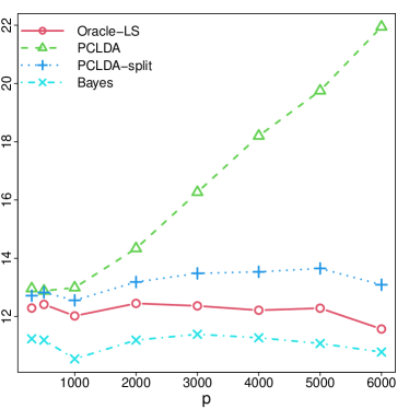
Figure 1: Illustration of the advantage of constructing from an independent dataset: PCLDA represents the PC-based classifier based on while PCLDA-split uses that is constructed from an independent . Oracle-LS is the oracle benchmark that uses both and while Bayes represents the risk of using the oracle Bayes rule. The y-axis represents the misclassification errors in percentage. We fix and and keep fixed, while we let grow. We refer to Section 6 for detailed data generating mechanism. - (c)
Conditions and are common in the analysis of factor models with a diverging number of features (Stock and Watson, 2002a; Bai and Li, 2012; Fan et al., 2013). For instance, holds when eigenvalues of are bounded and a fixed proportion of rows of are i.i.d. realizations of a sub-Gaussian random vector with covariance matrix having bounded eigenvalues as well. Nevertheless, consistency of the PC-based classifiers only requires for and for , both of which are much milder conditions.
5.3 Optimality of the PC-based LDA by sample splitting
We now show that the PC-based LDA by sample splitting achieves the minimax lower bounds in Theorem 3, up to multiplicative logarithmic factors of . Recalling that (2.3), for any , one has , , and . Based on Theorem 10, we have the following corollary for the classifier that uses . Its proof can be found in Appendix A.5.4. We use the notation for inequalities that hold up to a multiplicative logarithmic factor of . Recall from (2.4).
Corollary 11.
Under model (1.1), assume (i) – (v), and for some constants . For any , with probability , the classifier that uses satisfies the following statements.
-
(1)
If , then
-
(2)
If , and additionally, and as , then
-
(3)
If as , then
6 Simulation study
We conduct various simulation studies in this section to compare the performance of our proposed algorithm with other competitors. For our proposed algorithm, we call it PCLDA standing for the Principal Components based LDA. The name PCLDA- is reserved when the true is used as input. When is estimated by , we use PCLDA- instead. We call PCLDA-CF- the PCLDA with -fold cross-fitting. We consider in our simulation as suggested by Chernozhukov et al. (2018). To set a benchmark for PCLDA-CF-, we use PCLDA-split that uses an independent copy of to compute . On the other hand, we compare with the nearest shrunken centroids classifier (PAMR) (Tibshirani et al., 2002), the -penalized linear discriminant (PenalizedLDA) (Witten and Tibshirani, 2011) and the direct sparse discriminant analysis (DSDA) (Mai et al., 2012)111PAMR, PenalizedLDA and DSDA are implemented in the R packages pamr, penalizedLDA and TULIP, respectively.. Finally, we choose the performance of the oracle procedure (Oracle-LS) as benchmark in which Oracle-LS uses both and to estimate , and the classification rule in (3.3).
We generate the data as follows. First, we set , and . The parameter controls the signal strength in (2.2). We generate by independently sampling its diagonal elements from Unif(1,3) and set its off-diagonal elements as
The covariance matrix is generated in the same way, except we set . The rows of are generated independently from . Entries of are generated independently from . The training data , and are generated according to model (1.1) and (1.3). In the same way, we generate 100 data points that serve as test data for calculating the (out-of-sample) misclassification error for each algorithm.
In the sequel, we vary the dimensions and as well as the signal strength in (2.2), one at a time. For each setting, we repeat the entire procedure 100 times and averaged misclassification errors for each algorithm are reported.
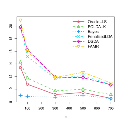
6.1 Vary the sample size
We set , , and vary within . The left-panel in Figure 2 shows the averaged misclassification error (in percentage) of each algorithm on the test data sets. Since consistently estimates , we only report the performance of PCLDA-. We also exclude the performance of PCLDA-split and PCLDA-CF- since they all have similar performance as PCLDA-222This is as expected since our data generating mechanism ensures in which case PCLDA-split has no clear advantage comparing to PCLDA- (see, discussions after Theorem 10).. The blue line represents the optimal Bayes error. All algorithms perform better as the sample size increases. As expected, Oracle-LS is the best because it uses the true and . Among the other algorithms, PCLDA- has the closest performance to Oracle-LS in all settings. The gap between PCLDA- and Oracle-LS does not close as increases. According to Theorem 9, this is because such a gap mainly depends on which does not vary with .
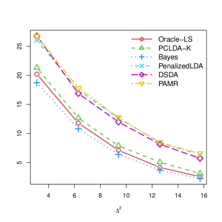
6.2 Vary the signal strength
We fix , , and vary within . As a consequence, the signal strength varies within . The right-panel of Figure 2 depicts the averaged misclassification errors of each algorithm. For the same reasoning as before, we exclude PCLDA-, PCLDA-CF- and PCLDA-split. It is evident that all algorithms have better performance as the signal strength increases. Among them, PCLDA- has the closest performance to Oracle-LS and Bayes in all settings.
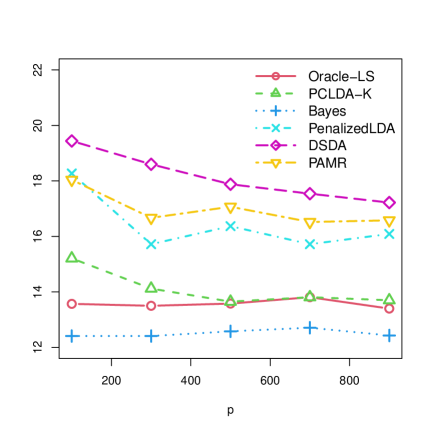
6.3 Vary the feature dimension
We examine the performance of each algorithm when the feature dimension varies across a wide range. Specifically, we fix , , and vary within . Figure 3 shows the misclassification errors of each algorithm. The performance of PCLDA- improves and gets closer to that of Oracle-LS as increases, in line with Theorem 9. The gap between Oracle-LS and Bayes is due to the fact that both and are held fixed.
7 Real data analysis
To further illustrate the effectiveness of our proposed method, we analyze three popular gene expression datasets (leukemia data, colon data and lung cancer data)333Leukemia data is available at www.broad.mit.edu/cgi-bin/cancer/datasets.cgi. Colon data is available from the R package plsgenomics. Lung cancer data is available at www.chestsurg.org., which have been widely used to test classification methods, see, for instance, Alon et al. (1999); Singh et al. (2002); Nguyen and Rocke (2002); Dettling (2004) and also, the more recent literature, Fan and Fan (2008); Mai et al. (2012); Cai and Zhang (2019a). These datasets contain thousands or even over ten-thousand features with around one hundred samples (see Table 1 for the summary). In such challenging settings, LDA-based classifiers that are designed for high-dimensional data are not only easy to interpret but also have competing and even superior performance than other, highly complex classifiers such as classifiers based on kernel support vector machines, random forests and boosting (Dettling, 2004; Mai et al., 2012).
| Data name | (category) | (category) | ||
|---|---|---|---|---|
| Leukemia | 7129 | 72 | 47 (acute lymphoblastic leukemia) | 25 (acute myeloid leukemia) |
| Colon | 2000 | 62 | 22 (normal) | 40 (tumor) |
| Lung cancer | 12533 | 181 | 150 (adenocarcinoma) | 31 (malignant pleural mesothelioma) |
Since the goal is to predict a dichotomous response, for instance, whether one sample is a tumor or normal tissue, we compare the classification performance of each algorithm. For all three data sets, the features are standardized to zero mean and unit standard deviation. For each dataset, we randomly split the data, within each category, into 70% training set and 30% test set. Different classifiers are fitted on the training set and their misclassification errors are computed on the test set. This whole procedure is repeated 100 times. The averaged misclassification errors (in percentage) as well as their standard deviations of each algorithm are reported in Table 2. Our proposed PC-based LDA classifiers have the smallest misclassification errors over all datasets. Although PCLDA-CF-5 only has the second best performance in Colon and Lung cancer data sets, its performance is very close to that of PCLDA-.
| PCLDA- | PCLDA-CF-5 | DSDA | PenalizedLDA | PAMR | |
|---|---|---|---|---|---|
| Leukemia | 3.57 (0.036) | 3.04 (0.032) | 5.52 (0.044) | 3.91 (0.043) | 4.61 (0.039) |
| Colon | 16.37 (0.077) | 18.11 (0.082) | 18.11 (0.07) | 33.95 (0.086) | 19.00 (0.089) |
| Lung cancer | 0.55 (0.008) | 0.60 (0.009) | 1.69 ( 0.017) | 1.80 (0.026) | 0.91 (0.011) |
8 Extension to multi-class classification
In this section, we discuss how to extend the previously discussed procedure to multi-class classification problems in which has classes, , for some positive integer , and model (1.3) holds, that is,
| (8.1) |
In particular, the covariance matrices for the classes are the same.
For a new point , the oracle Bayes rule assigns it to if and only if
| (8.2) |
where
| (8.3) |
Notice that and, for any , the proof of (3.2) reveals that,
| (8.4) |
with , ,
| (8.5) | ||||
In view of (8) and (8.4), for a new point and any matrix with , we propose the following multi-class classifier
| (8.6) |
where and, for any ,
| (8.7) |
with
Here and are the non-parametric estimates as (3.6) and both the submatrix of and the response vector correspond to samples with label in . Note that is encoded as for observations with label and otherwise.
To analyze the classifier in (8.6), its excess risk depends on
| (8.8) |
as well as as defined in (4.7). Here . Analogous to (4.9), for some constant , define
| (8.9) |
For ease of presentation, we also assume there exists some sequence and some absolute constants such that
| (8.10) |
The following theorem extends Theorem 7 to multi-class classification by establishing rates of convergence of the excess risk of in (8.6) for a general .
Theorem 12.
Proof.
The proof can be found in Appendix A.6. ∎
Condition (8.10) is only assumed to simplify the presentation. It is straightforward to derive results based on our analysis when the separation is not of the same order for all . For the third case, , our proof also allows to establish different convergence rates depending on whether or not and are distinct for each , analogous to the last two cases of Theorem 7. However, we opt for the current presentation for succinctness.
Theorem 12 immediately leads to the following corollary for the PC-based classfiers that use and . Furthermore, Theorem 8 also ensures that similar guarantees can be obtained for the classifiers in (8.6) that use and .
Corollary 13.
Proof.
See Appendix A.6.3. ∎
Remark 14.
Multi-class classification problems based on discriminant analysis have been studied, for instance, by Witten and Tibshirani (2011); Clemmensen et al. (2011); Mai et al. (2019); Cai and Zhang (2019b). Theoretical guarantees are only provided in Mai et al. (2019) and Cai and Zhang (2019b) under the classical LDA setting for moderate / large separation scenarios, , and for fixed , the number of classes. Our results fully characterize dependence of the excess risk on and also cover the weak separation case, . On the other hand, our proposed procedure solves a long standing issue on generalizing regression-based classification methods (Hastie et al., 2009; Izenman, 2008; Mai et al., 2012) in the classical binary LDA setting to handle multi-class classification.
Remark 15.
The classifier in (8.6) chooses as the baseline. In practice, we recommend taking each class as the baseline one at the time and averaging the predicted probabilities. Specifically, it is easy to see that, for any baseline choice and for any ,
where is defined analogous to (8) with in lieu of . Therefore, for any new data point , the averaged version of the classifier in (8.6) is
with defined analogous to (8.7). The empirical finite sample performance and theoretical analysis of this classifier will be studied elsewhere.
Appendix
Appendix A Main proofs
A.1 Proofs of Section 2
A.1.1 Proof of Lemma 1
We observe that
| (A.1) | ||||
In the derivation (A.1.1) above, the infima are taken over all measurable functions and , and note that the second inequality uses the independence between and . ∎
A.1.2 Proof of Lemma 2
We define
| (A.2) |
From standard LDA theory (Izenman, 2008, pp 241-244),
which simplifies for to . Hence, we have
Since, by an application of the Woodbury identity,
| (A.3) |
we have
| (A.4) |
with . Since
and the function is increasing for , we further find that
| (A.5) |
Finally, using the mean value theorem, we find
Our claim of the upper bound thus follows from for any .
To prove the lower bound of , note that
This implies
Similarly, by the mean value theorem and from (A.4),
The result follows from this inequality and for any . ∎
A.2 Proof of Proposition 4
We prove Proposition 4 by proving the following more general result. Define, for any scalar ,
| (A.6) | ||||
Lemma 14.
Proof.
To prove the first statement, write
| (A.7) |
It suffices to show that, for any ,
| (A.8) |
and
| (A.9) |
To show (A.9), observe that (see, Fact 1)
| (A.10) |
By the Woodbury formula,
This gives
| (A.11) |
which implies
| (A.12) |
Hence (A.9) follows as
We proceed to show (A.8). By using (A.10) and the Woodbury formula again,
This proves (A.8) and completes the proof of the first statement.
To prove the second statement, by definition and the choice of ,
On the other hand,
proving our claim.
The last statement follows immediately from (A.8) with . ∎
A.3 Proofs of Section 4
A.3.1 Proof of Theorem 5
Since is independent of , we treat quantities that are only related with fixed throughout the proof. Recall the definitions of and in (4.1). By definition,
and
Recall that and write for the p.d.f. of at the point for . We have
The penultimate step uses the assumption that is independent of both and . Notice that
with
from Lemma 14 and (A.7). This implies the identity
Define, for any , the event
| (A.13) |
We obtain
In the last step we use the basic inequality for all together with and on the event .
By using analogous arguments and from the identity
we find is equal to
Combining the bounds for and and using , we conclude that
Using the fact that
the proof easily follows. ∎
A.3.2 Proof of Proposition 6
Recall that
The proof of Proposition 6 consists of two parts: we first show that, for any , with probability at most ,
| (A.14) | ||||
Notice that randomness of the right-hand side only depends on . We then prove in Lemma 15 that with probability ,
| (A.15) |
which together with (A.14) yields the claim.
To prove (A.14), starting with
we observe that and are independent of and . Since given is subGaussian with parameter , we find that, for any ,
| (A.16) |
To bound , by conditioning on and , and by recalling that , we have
for all , where
By the Cauchy-Schwarz inequality and (A.10),
Furthermore, by (A.11), we have
These bounds of and yield that, for any ,
By the same arguments, the above also holds by conditioning on , hence further holds by unconditioning on . Together with (A.16), the proof of (A.14) is complete by taking , concluding the proof of Proposition 6. ∎
Lemma 15.
Proof.
By definition,
We proceed to bound and separately.
Bounding . By recalling that, for any ,
| (A.17) |
we have
The last step uses
and Cauchy-Schwarz inequality. By invoking Lemma 31 and using
| (A.18) |
from (vi), we further have
with probability . Lemma 30 yields
| (A.19) |
After collecting the above terms and using Fact 1 and , we obtain
with probability . Notice that
| by (A.19) | ||||
and, similarly,
Then use Lemma 32 to obtain
which further implies
with probability . Therefore, with the same probability, we have
| (A.20) |
In the last step, we also use from Fact 1 and to collect terms.
A.3.3 Proof of Theorem 7
On the event , we use the result of Theorem 5 with . It remains to bound from above
| (A.22) |
with
By the mean-value theorem, we have the bound
We consider three scenarios:
(1) . In this case, and , so that
(2) . In this case, , , whence with if , and
(3a) and and are distinct. In this case , , , , whence and
In view of the above three cases, on the event , the proof is complete by invoking Theorem 5. ∎
A.4 A general tool of bounding and for a generic choice
In this section, we provide a general result of establishing and for in (3.4) with . Here is any matrix and its dimension is also allowed to be random. Recall that is the projection matrix onto the column space of and . Define
For any , the following theorem bounds and in terms of the two quantities above as well as and
| (A.23) |
Theorem 16.
The following theorem states an alternative bound of which is potentially smaller than that in Theorem 16. It requires the following event,
| (A.25) |
where is some sufficiently small constant.
Theorem 17.
Under conditions of Theorem 16, assume for some . Then, on the event , the following holds with probability ,
We prove Theorem 16 below and the proof of Theorem 17 follows from the same argument in conjunction with Lemma 20.
Proof of Theorem 16.
A.4.1 Key lemmas used in the proof of Theorems 16 & 17
Lemma 18.
Under conditions of Theorem 16, with probability ,
Proof.
Lemma 19.
Suppose for some constant . On the event , the following inequalities hold with probability for any ,
Proof.
We start by proving the first three claims. By definition, for any ,
where the last equality uses . Take to obtain
| (A.28) |
where
| I | |||
| II |
On the event , by using , we further have
| I | |||
Note that
and
| (A.29) |
We conclude
Regarding II, one similarly has
with probability . The last step invokes Lemma 32. The first claim follows after we combine these bounds of I and II.
To prove the second claim. From (A.29) and , we find
where . Adding and subtracting gives
To bound from above , write the SVD of as where and are orthogonal matrices with . We have
| (A.30) |
where we used for any matrix in , in and
in . By collecting terms, the second result follows from (A.23) and Lemma 32.
Regarding the third result, the bound follows immediately from
and (A.4.1). To prove the other bound, start with
Display (A.4.1) and Lemma 33 ensure that, with probability , the second term on the right hand side is bounded by
| (A.31) |
For the first term, we have, on , with probability ,
| (A.32) |
where the last step uses Lemma 18 and together with (A.11). It remains to bound which is less than
| by (A.4.1). | |||
Observe that, on the event ,
| (A.33) |
The last step invokes Lemma 32 together with (A.4.1). Combining (A.31) with (A.4.1) and (A.4.1) yields the desired result. ∎
On the event defined in (A.25), the following lemma states potentially faster rates of the quantities analyzed in Lemma 19. Recall that (A.23).
Lemma 20.
Suppose for some constant . On the event , the following inequalities hold with probability for any
A.5 Proofs of Section 5
A.5.1 Proof of Theorem 8
We show with probability tending to one. Let . Under conditions of Theorem 8, Proposition 8 in Bing et al. (2021) shows that holds on the event
and . Thus it remains to prove on the event . From Corollary 10 of Bing and Wegkamp (2019), we need to verify
For the left-hand-side, invoking in (A.26) gives
Regarding the right-hand-side, by invoking and using
from (3.8), it can be bounded from above by
The proof is then completed by observing that
is sufficiently small. ∎
A.5.2 Proof of Theorem 9
We first prove the result when as stated in Remark 10. According to Theorem 7, it suffices to invoke Theorem 16 with , and together with a bound for . First, by using
| (A.34) |
for some constant , and by using Weyl’s inequality, we find that
| (A.35) |
with probability . Second, with the same probability, we find that
| (A.36) |
using Weyl’s inequality, inequality (A.35), our assumption and the event together with . Finally, invoke Lemma 21 to identify
in Theorem 16 as well as
with probability .
Plugging into the above upper bounds yields (5.5), completing the proof of Theorem 9 for .
When , Lemma 21 ensures that in (A.25) holds with probability such that we can invoke Theorem 17 for bounding . To this end, first note that, with probability ,
which together with and imply that and . Then invoking Theorem 17 gives that, with probability ,
We conclude (5.4) after collecting terms. ∎
Lemma 21.
Under conditions of Theorem 9, with probability , one has
A.5.3 Proof of Theorem 10
Similar as the proof of Theorem 9, we aim to invoke Theorem 17 with and . By invoking Lemma 21 with and replaced by and , respectively, we have
| (A.37) |
with probability . The event in (A.25) of Theorem 17 thus holds under . Furthermore, since is independent of , hence independent of , an application of Lemma 35 yields
where satisfies . It then follows that, with the same probability,
| (A.38) |
Similarly, the same proof for the last result of Lemma 32 with replaced by yields that, with probability ,
implying
To bound from below , we first find that
Since, with probability ,
where the last step uses (A.10) and , by also using and (A.34) together with , we conclude
| (A.39) |
Then invoking Theorem 17 gives that, with probability ,
implying that
We used in the last step. The proof is complete. ∎
A.5.4 Proof of Corollary 11
A.6 Proofs of Section 8
For notational convenience, define
| (A.40) |
In particular, for any , we have
Further recall that
For any , define the event
| (A.41) |
Finally, we write for simplicity
| (A.42) |
A.6.1 Proof of Theorem 12
By definition, we start with
Recall that is the p.d.f. of for each . Repeating arguments in the proof of Theorem 7 gives
with defined in (A.40). Since
| (A.43) |
the event implies
By repeating the arguments of analyzing term in the proof of Theorem 7, we obtain that, for any ,
| (A.44) | ||||
where
The penultimate step uses the fact that
while the last step applies the mean-value theorem. By choosing
and invoking condition (8.10) and , we find that:
-
(a)
If , then
-
(b)
If , then ensures that hence
- (c)
In view of cases (a) – (c), since the event implies
it remains to prove that, with probability , the right-hand side of the above display is no greater than . This is proved by combining Lemmas 22 and 23. ∎
A.6.2 Lemmas used in the proof of Theorem 12
The following lemma establishes the probability tail of the event defined in (A.41) for , a random sequence defined below whose randomness only depends on . Recall and from (8.8). Set
| (A.45) | ||||
Lemma 22.
Under conditions of Theorem 12, we have,
Proof.
Pick any . By definition,
where
| I | |||
| II | |||
| III | |||
First, notice that the numerator of I is bounded from above by
which, by the arguments of proving Proposition 6 and by conditioning on for any , with probability for any , is no greater than
In the second step, we also used
Again, by the arguments of proving Proposition 6, with probability for any ,
Taking for some positive constant in these two bounds yields the claim. ∎
Lemma 23.
Under conditions of Theorem 12, we have
Proof.
We first bound from above the numerators of the last two terms in defined in (A.45). By Lemma 30 and for all , we have
for some constant . With the same probability, using further yields that, for any ,
as well as
Pick any . By following the same arguments of proving Lemma 15 and using the condition , we have, with probability ,
| (A.46) |
By taking the union bounds over , the above bound also holds for all with probability .
It remains to bound from below . To this end, repeating arguments of proving Lemma 14 gives
and, by recalling that ,
It then follows that
Thus, by (A.6.2), condition (8.10) and condition we find that, with probability ,
Combining the last display with (A.6.2) gives that, with probability ,
completing the proof. ∎
A.6.3 Proof of Corollary 13
Appendix B Proof of the minimax lower bounds of the excess risk
Proof of Theorem 3.
Recall that . It suffices to consider Further recall that , and for sufficiently small positive constants and .
To prove Theorem 3, it suffices to consider the Gaussian case. Specifically, for any , consider
| (B.1) |
with
In this case, the Bayes rule of using is
| (B.2) |
For any classifier , one has
Lemma 2 together with ensures that, for any ,
| (B.3) |
Note that has the smallest risk over all measurable functions . We proceed to bound from below by splitting into two scenarios depending on the magnitude of .
Case 1: . We may assume for simplicity. It suffices to show
| (B.4) |
where
| (B.5) |
and
| (B.6) |
We take the leading constant in small enough such that
-
(a)
, where are defined in Theorem 3.
- (b)
These two requirements will become apparent soon.
To prove (B.4), we first introduce another loss function
| (B.7) |
We proceed to bound from below by using . By following the same arguments in the proof of Theorem 5 with replaced by , one can deduce that
where
For any ,
| I | |||
Similarly,
Combine these two lower bounds, the identity and the inequality for to obtain,
for any . From (A.2), we see that , and we easily find
and, similarly,
An application of the mean value theorem yields
| (B.8) |
for
Then, for , we easily find from (B.8) that
Hence, for any , we proved that
| (B.9) | ||||
Next, choose
with defined in (B.6). Inequality holds by using , , and requirement (a) of the constant in the definition (B.6) of .
In the proof of the lower bounds (B.14) and (B.15) below, we consider subsets of such that, for any ,
| (B.10) |
This implies
| (B.11) |
provided that , and, using (B.5),
| (B.12) |
Note that (B.10) further implies . Then, by plugging into (B.9) and using (B.11) and (B.12), we find
| (B.13) | ||||
In the next two sections we prove the inequalities
| (B.14) | ||||
| (B.15) |
for some positive constants and .
By using requirement (b) for the leading constant
in the definition (B.6) of , we can conclude from the final lower bound (B.13) the proof of Theorem 3 for .
Case 2: . We further consider two cases and recall that
When , we now prove the lower bound . By choosing
| (B.16) |
in (B.8) for some constant and by using , and , we find
From (B.14) and (B.15), it follows that
for some constant depending on and . Therefore, by using and and taking sufficiently small, we conclude
The above display together with (B.3) proves the lower bound .
B.1 Proof of (B.15)
Proof.
We aim to invoke the following lemma to obtain the desired lower bound. The lemma below follows immediately from the proof of Proposition 1 in Azizyan et al. (2013) together with Theorem 2.5 in Tsybakov (2009).
Lemma 24.
Let and . For some constant , and any classifier , if for all , and implies for all , then
To this end, we start by describing our construction of hypotheses of defined in (2.3). Without loss of generality, we assume and . We consider a subspace of where . By further writing with , we consider
| (B.17) |
where
| (B.18) |
with
| (B.19) |
for some constants and . Here are chosen according to the hypercube construction in Lemma 25 with . It is easy to see that for all . Lemma 26 below collects several useful properties of .
B.1.1 Lemmas used in the proof of (B.15)
The following lemma is adapted from Vu and Lei (2013, Lemma A.5).
Lemma 25 (Hypercube construction).
Let be an integer. There exist with the following properties:
-
1.
for all , and
-
2.
, where is an absolute constant.
Proof.
The case for is proved in Vu and Lei (2013, Lemma A.5) by taking . For , one can choose , for , and , for , such that and . Here represents the set of canonical vectors in . For , one can simply take for . ∎
Lemma 26.
Proof.
Let , for , denote the distribution of parametrized by . The following lemma provides upper bounds of the KL-divergence between and .
Lemma 27 (KL-divergence).
For any , let
with , and . Then
Proof.
Since contains i.i.d. copies of , it suffices to prove
By the formula of KL-divergence between two multivariate normal distributions,
From Vu and Lei (2013, Lemmas A.2 & A.3),
For , by using part (i) of Lemma 26 together with
from (B.18), we find
Combining the bounds of and and using complete the proof. ∎
Recall that is defined in (B.7). The following lemma establishes lower bounds of for any measurable .
Lemma 28.
Proof.
Pick any and any . For simplicity, we write and with corresponding and . We also write and . The proof consists of three steps:
-
(a)
Bound from below by a -dimensional integral;
-
(b)
Reduce the -dimensional integral to a -dimensional integral;
-
(c)
Bound from below the -dimensional integral.
Step (a)
Step (b)
In the following, we provide a lower bound for
Recall from (B.18) and (B.21) that
Further note from part (ii) of Lemma 26 that
Plugging these expressions in yields
Let such that
| (B.24) |
Such an exists since has rank and . By changing variables and by writing , we obtain
Denote
| (B.25) |
Notice that by (B.23). We further have
where is the first submatrix of . Recall that and on the area of integration we have
Splitting into two parts further gives
Step (c)
We bound from below first. Denote
| (B.26) |
where the second equality uses the Sherman-Morrison formula and the third equality is due to the fact that
| by (B.24) and (B.25) | |||||
| by (B.18). | (B.27) |
Further observe that
We obtain
By changing of variables again and writing
for simplicity, one has
Note that, the integral is simply the area within the half unit circle intersected by vectors and . We thus conclude
where , and denotes the length of the arc between and .
We proceed to calculate . First note that
Since
we obtain
The penultimate step uses the orthogonality between and . Since
which can be bounded by a sufficiently small constant, we have hence . Finally, similar arguments yield
We thus have, after a bit algebra,
hence
implying that
Following the same line of reasoning, we can derive the same lower bound for . We conclude that
which completes the proof. ∎
B.2 Proof of (B.14)
The proof of (B.14) follows the same lines of reasoning as the proof of (B.15). To construct hypotheses of , we consider
| (B.28) |
with and
| (B.29) |
Here for are again chosen according to Lemma 25 with and
| (B.30) |
for some constant and . Notice that for all , so that . From part (iii) of Lemma 26, we also have
Next, to invoke Lemma 24, it remains to verify
-
(1)
for all ;
-
(2)
, for all and any , with
To prove (1), note that the distribution of parametrized by is
with and . Following the arguments in the proof of Lemma 27 yields
| by (B.20), | |||||
| (B.31) | |||||
Claim (1) then follows from by using Lemma 25 and the additivity of KL divergence among independent distributions. Since claim (2) is proved in Lemma 29, the proof is complete.∎
Lemma 29.
Proof.
The proof uses the same reasoning for proving Lemma 28. Pick any and write and . From (B.1.1), one has
where . Let such that
By changing variable and writing , we find
where is the first matrix of
By another change of variable and the same reasoning in the proof of Lemma 28,
where
Since
and
| by (B.2) | ||||
we conclude
Using completes the proof. ∎
Appendix C Technical lemmas
Consider . This section contains some basic relations between and , collected in Fact 1, as well as some useful technical lemmas. For simplicity, we write for from now on.
Fact 1.
Let . One has
Additionally, for any , one has
As a result,
The following lemma provides concentration inequalities of .
Lemma 30.
For any and all ,
In particular, if , then for any ,
Furthermore, if for some sufficiently large constant , then
Proof.
The first result follows from an application of the Bernstein inequality for bounded random variables. The second one follows by choosing and the last one can be readily seen from the second display. ∎
C.1 Deviation inequalities of quantities related with
Recall that , and . Let the centered as
The following lemma provides concentration inequalities of and some useful bounds related with the random matrices and .
Lemma 31.
Suppose that model (1.3) holds.
-
(i)
For any deterministic vector , for all ,
-
(ii)
-
(iii)
With probability ,
-
(iv)
For any deterministic vector , with probability ,
-
(v)
With probability ,
-
(vi)
Assume for some sufficiently small constant . With probability ,
holds for some constants depending on only.
-
(vii)
Under conditions of (vi), there exists some absolute constants such that, with probability , one has
and
Proof.
Without loss of generality, we assume such that .
To prove (i), by conditioning on , the fact that are i.i.d. implies that, for all and any deterministic ,
The statement above yields (i) by unconditioning on .
To show part (ii), by taking and in (i) together with the union bounds over , we conclude
with probability . The last inequality also uses , deduced from (A.10).
To prove part (iii), without loss of generality, assume . By adding and subtracting terms and using
| (C.1) |
we obtain the identity
where in the third line we used and . Therefore, by recalling that (A.27) and (3.6),
Invoking part (ii) and Lemma 30, together with
| (C.2) |
deduced from (A.11), completes the proof of (iii).
To prove (iv), notice that
Since (A.10), (C.1) and Fact 1 imply
we obtain, for any ,
| (C.3) |
Notice that
with and . An application of Lemma 36 yields
with probability . By further invoking Lemma 30 and part (i), we conclude
with probability . Since
from the Cauchy-Schwarz inequality, by noting that
and invoking Fact 1 for
we conclude, with the same probability,
where we used (C.2) in the last line.
Next, we prove (v) by bounding from above
Recalling that (C.1), an application of Lemma 36 yields
with probability . The result follows by the same arguments of proving (iv) and also by noting that the other terms are bounded uniformly over .
As a result of (v), part (vi) follows from the bound (A.18) and Weyl’s inequality.
Finally, to prove (vii), observe that
with . Consequently,
Invoking (iii) and (v) gives the desired result. The bounds on eigenvalues of follow from Weyl’s inequality. ∎
C.2 Deviation inequalities of quantities related with
The following lemma provides deviation inequalities for various quantities related with . Recall that
Further recall that is defined in (A.26).
Lemma 32.
Grant assumption (i) – (vi) and . We have the following results.
Here is some absolute constant.
Proof.
Recall that . Invoke Lemma 35 with and together with , and to obtain
Similarly, by invoking Lemma 35 and using , the second result follows from
| (C.4) |
with probability at least .
Regarding the third result, since given is -subGaussian, Lemma 34 gives
| (C.5) |
with probability . The last inequality in (C.2) uses .
To prove the fourth result, let with . Further let be the -net of . By the properties of , we have
Furthermore,
| (C.6) |
By (iii) of Lemma 31 and (C.2), the second term can be bounded from above, uniformly over , as
with probability .
It remains to show that the same bound holds for the first term in (C.2). Since and are independent, conditioning on , we know is sub-Gaussian with sub-Gaussian constant equal to
recalling that . Thus, is sub-Gaussian with sub-Gaussian constant equal to
We conclude that, for each ,
The result follows by choosing for some sufficiently large constant , taking a union bounds over together with , and invoking (v) of Lemma 31.
The following lemma analyzes some of the quantities in Lemma 32 with replaced by any estimator .
Lemma 33.
Under conditions of Lemma 32, for any , we have
Proof.
In view of Lemma 32, the first and third results follow from the triangle inequality. For the second claim, it suffices to bound from above
Invoking gives the claim. ∎
Appendix D Auxiliary lemmas
The following lemma is the tail inequality for a quadratic form of sub-Gaussian random vectors. We refer to Bing et al. (2021, Lemma 16) for its proof, also see, Lemma 30 in Hsu et al. (2014).
Lemma 34.
Let be a sub-Gaussian random vector. For all symmetric positive semi-definite matrices , and all ,
The following lemma provides an upper bound on the operator norm of where is a random matrix and its rows are independent sub-Gaussian random vectors. It is proved in Lemma 22 of Bing et al. (2021).
Lemma 35.
Let be a matrix with rows that are independent sub-Gaussian random vectors with identity covariance matrix. Then for all symmetric positive semi-definite matrices ,
Another useful concentration inequality of the operator norm of the random matrices with i.i.d. sub-Gaussian rows is stated in the following lemma. This is an immediate result of Vershynin (2012, Remark 5.40).
Lemma 36.
[Bing et al. (2021, Lemma 16)] Let be by matrix whose rows are i.i.d. sub-Gaussian random vectors with covariance matrix . Then for every , with probability at least ,
with where and are positive constants depending on .
References
- Alon et al. (1999) Alon, U., Barkai, N., Notterman, D. A., Gish, K., Ybarra, S., Mack, D. and Levine, A. J. (1999). Broad patterns of gene expression revealed by clustering analysis of tumor and normal colon tissues probed by oligonucleotide arrays. Proceedings of the National Academy of Sciences 96 6745–6750.
- Antoniadis et al. (2003) Antoniadis, A., Lambert-Lacroix, S. and Leblanc, F. (2003). Effective dimension reduction methods for tumor classification using gene expression data. Bioinformatics 19 563–570.
- Azizyan et al. (2013) Azizyan, M., Singh, A. and Wasserman, L. (2013). Minimax theory for high-dimensional gaussian mixtures with sparse mean separation. In Advances in Neural Information Processing Systems (C. J. C. Burges, L. Bottou, M. Welling, Z. Ghahramani and K. Q. Weinberger, eds.), vol. 26. Curran Associates, Inc.
- Bai and Li (2012) Bai, J. and Li, K. (2012). Statistical analysis of factor models of high dimension. Ann. Statist. 40 436–465.
- Bai and Ng (2008) Bai, J. and Ng, S. (2008). Forecasting economic time series using targeted predictors. Journal of Econometrics 146 304 – 317. Honoring the research contributions of Charles R. Nelson.
- Bair et al. (2006) Bair, E., Hastie, T., Paul, D. and Tibshirani, R. (2006). Prediction by supervised principal components. Journal of the American Statistical Association 101 119–137.
- Barker and Rayens (2003) Barker, M. and Rayens, W. (2003). Partial least squares for discrimination. Journal of Chemometrics: A Journal of the Chemometrics Society 17 166–173.
- Barshan et al. (2011) Barshan, E., Ghodsi, A., Azimifar, Z. and Jahromi, M. Z. (2011). Supervised principal component analysis: Visualization, classification and regression on subspaces and submanifolds. Pattern Recognition 44 1357–1371.
- Belloni et al. (2012) Belloni, A., Chen, D., Chernozhukov, V. and Hansen, C. (2012). Sparse models and methods for optimal instruments with an application to eminent domain. Econometrica 80 2369–2429.
- Biau et al. (2003) Biau, G., Bunea, F. and Wegkamp, M. H. (2003). Functional classification in hilbert spaces. IEEE Transactions on Information Theory 11 1045 – 1076.
- Bing et al. (2020) Bing, X., Bunea, F., Ning, Y. and Wegkamp, M. (2020). Adaptive estimation in structured factor models with applications to overlapping clustering. The Annals of Statistics 48 2055–2081.
- Bing et al. (2021) Bing, X., Bunea, F., Strimas-Mackey, S. and Wegkamp, M. (2021). Prediction under latent factor regression: Adaptive pcr, interpolating predictors and beyond. Journal of Machine Learning Research 22 1–50.
- Bing and Wegkamp (2019) Bing, X. and Wegkamp, M. H. (2019). Adaptive estimation of the rank of the coefficient matrix in high-dimensional multivariate response regression models. Ann. Statist. 47 3157–3184.
- Boulesteix (2004) Boulesteix, A.-L. (2004). Pls dimension reduction for classification with microarray data. Statistical applications in genetics and molecular biology 3.
- Cai and Liu (2011) Cai, T. and Liu, W. (2011). A direct estimation approach to sparse linear discriminant analysis. Journal of the American Statistical Association 106 1566–1577.
- Cai and Zhang (2019a) Cai, T. and Zhang, L. (2019a). High dimensional linear discriminant analysis: optimality, adaptive algorithm and missing data. Journal of the Royal Statistical Society: Series B (Statistical Methodology) 81 675–705.
- Cai and Zhang (2019b) Cai, T. T. and Zhang, L. (2019b). A convex optimization approach to high-dimensional sparse quadratic discriminant analysis.
- Chernozhukov et al. (2018) Chernozhukov, V., Chetverikov, D., Demirer, M., Duflo, E., Hansen, C., Newey, W. and Robins, J. (2018). Double/debiased machine learning for treatment and structural parameters. The Econometrics Journal 21 C1–C68.
- Chiaromonte and Martinelli (2002) Chiaromonte, F. and Martinelli, J. (2002). Dimension reduction strategies for analyzing global gene expression data with a response. Mathematical Biosciences 176 123–144.
- Clemmensen et al. (2011) Clemmensen, L., Hastie, T., Witten, D. and Ersbøll, B. (2011). Sparse discriminant analysis. Technometrics 53 406–413.
- Dai et al. (2006) Dai, J. J., Lieu, L. and Rocke, D. (2006). Dimension reduction for classification with gene expression microarray data. Statistical applications in genetics and molecular biology 5.
- Dettling (2004) Dettling, M. (2004). BagBoosting for tumor classification with gene expression data. Bioinformatics 20 3583–3593.
- Fan and Fan (2008) Fan, J. and Fan, Y. (2008). High-dimensional classification using features annealed independence rules. The Annals of Statistics 36 2605 – 2637.
- Fan et al. (2013) Fan, J., Liao, Y. and Mincheva, M. (2013). Large covariance estimation by thresholding principal orthogonal complements. Journal of the Royal Statistical Society: Series B (Statistical Methodology) 75 603–680.
- Fan et al. (2017) Fan, J., Xue, L. and Yao, J. (2017). Sufficient forecasting using factor models. Journal of Econometrics 201 292 – 306.
- Ghosh (2001) Ghosh, D. (2001). Singular value decomposition regression models for classification of tumors from microarray experiments. In Biocomputing 2002. World Scientific, 18–29.
- Hadef and Djebabra (2019) Hadef, H. and Djebabra, M. (2019). Proposal method for the classification of industrial accident scenarios based on the improved principal components analysis (improved pca). Production Engineering 13 53–60.
- Hahn et al. (2013) Hahn, P. R., Carvalho, C. M. and Mukherjee, S. (2013). Partial factor modeling: Predictor-dependent shrinkage for linear regression. Journal of the American Statistical Association 108 999–1008.
- Hastie et al. (2009) Hastie, T., Tibshirani, R. and Friedman, J. (2009). The elements of statistical learning: data mining, inference and prediction. 2nd ed. Springer.
- Hotelling (1957) Hotelling, H. (1957). The relations of the newer multivariate statistical methods to factor analysis. British Journal of Statistical Psychology 10 69–79.
- Hsu et al. (2014) Hsu, D., Kakade, S. M. and Zhang, T. (2014). Random design analysis of ridge regression. Found. Comput. Math. 14 569–600.
- Izenman (2008) Izenman, A. J. (2008). Modern Multivariate Statistical Techniques: Regression, Classification, and Manifold Learning. Series: Springer Texts in Statistics.
- Jin et al. (2021) Jin, D., Henry, P., Shan, J. and Chen, J. (2021). Classification of cannabis strains in the canadian market with discriminant analysis of principal components using genome-wide single nucleotide polymorphisms. Plos one 16 e0253387.
- Li (2016) Li, H. (2016). Accurate and efficient classification based on common principal components analysis for multivariate time series. Neurocomputing 171 744–753.
- Ma et al. (2020) Ma, Z., Liu, Z., Zhao, Y., Zhang, L., Liu, D., Ren, T., Zhang, X. and Li, S. (2020). An unsupervised crop classification method based on principal components isometric binning. ISPRS International Journal of Geo-Information 9 648.
- Mai et al. (2019) Mai, Q., Yang, Y. and Zou, H. (2019). Multiclass sparse discriminant analysis. Statistica Sinica 29 97–111.
- Mai et al. (2012) Mai, Q., Zou, H. and Yuan, M. (2012). A direct approach to sparse discriminant analysis in ultra-high dimensions. Biometrika 99 29–42.
- Mallary et al. (2022) Mallary, C., Berg, C., Buck, J. R., Tandon, A. and Andonian, A. (2022). Acoustic rainfall detection with linear discriminant functions of principal components. The Journal of the Acoustical Society of America 151 A149–A149.
- Nguyen and Rocke (2002) Nguyen, D. V. and Rocke, D. M. (2002). Tumor classification by partial least squares using microarray gene expression data . Bioinformatics 18 39–50.
- Shao et al. (2011) Shao, J., Wang, Y., Deng, X. and Wang, S. (2011). Sparse linear discriminant analysis by thresholding for high dimensional data. The Annals of Statistics 39 1241 – 1265.
- Singh et al. (2002) Singh, D., Febbo, P. G., Ross, K., Jackson, D. G., Manola, J., Ladd, C., Tamayo, P., Renshaw, A. A., D’Amico, A. V., Richie, J. P., Lander, E. S., Loda, M., Kantoff, P. W., Golub, T. R. and Sellers, W. R. (2002). Gene expression correlates of clinical prostate cancer behavior. Cancer Cell 1 203–209.
- Stock and Watson (2002a) Stock, J. H. and Watson, M. W. (2002a). Forecasting using principal components from a large number of predictors. Journal of the American Statistical Association 97 1167–1179.
- Stock and Watson (2002b) Stock, J. H. and Watson, M. W. (2002b). Macroeconomic forecasting using diffusion indexes. Journal of Business & Economic Statistics 20 147–162.
- Tarigan and Van de Geer (2006) Tarigan, B. and Van de Geer, S. (2006). Classifiers of support vector machine type with complexity regularization. Bernoulli 12 1045 – 1076.
- Tibshirani et al. (2002) Tibshirani, R., Hastie, T., Narasimhan, B. and Chu, G. (2002). Diagnosis of multiple cancer types by shrunken centroids of gene expression. Proceedings of the National Academy of Sciences 99 6567–6572.
- Tsybakov (2004) Tsybakov, A. B. (2004). Optimal aggregation of classifiers in statistical learning. The Annals of Statistics 32 135–166.
- Tsybakov (2009) Tsybakov, A. B. (2009). Introduction to nonparametric estimation. Springer Series in Statistics. Springer, New York.
- Vershynin (2012) Vershynin, R. (2012). Introduction to the non-asymptotic analysis of random matrices. Cambridge University Press, 210 – 268.
- Vu and Lei (2013) Vu, V. Q. and Lei, J. (2013). Minimax sparse principal subspace estimation in high dimensions. The Annals of Statistics 41 2905–2947.
- Wegkamp and Yuan (2011) Wegkamp, M. and Yuan, M. (2011). Support vector machines with a reject option. Bernoulli 17 1368 – 1385.
- Witten and Tibshirani (2011) Witten, D. M. and Tibshirani, R. (2011). Penalized classification using fisher’s linear discriminant. Journal of the Royal Statistical Society: Series B (Statistical Methodology) 73 753–772.
- Yu et al. (2014) Yu, Y., Wang, T. and Samworth, R. J. (2014). A useful variant of the Davis–Kahan theorem for statisticians. Biometrika 102 315–323.