Deep-Learning-Based Precipitation Nowcasting with Ground Weather Station Data and Radar Data

Abstract

Recently, many deep-learning techniques have been applied to various weather-related prediction tasks, including precipitation nowcasting (i.e., predicting precipitation levels and locations in the near future). Most existing deep-learning-based approaches for precipitation nowcasting, however, consider only radar and/or satellite images as inputs, and meteorological observations collected from ground weather stations, which are sparsely located, are relatively unexplored. In this paper, we propose ASOC, a novel attentive method for effectively exploiting ground-based meteorological observations from multiple weather stations. ASOC is designed to capture temporal dynamics of the observations and also contextual relationships between them. ASOC is easily combined with existing image-based precipitation nowcasting models without changing their architectures. We show that such a combination improves the average critical success index (CSI) of predicting heavy (at least 10 mm/hr) and light (at least 1 mm/hr) rainfall events at 1-6 hr lead times by 5.7%, compared to the original image-based model, using the radar images and ground-based observations around South Korea collected from 2014 to 2020.

I Introduction

Recently, deep learning techniques, especially computer vision techniques, have been applied to forecasting various weather-related events, and such approaches [1, 2, 3, 4, 5, 6] often outperform traditional methods in the field. A representative example is precipitation nowcasting, which is short-term (e.g., at $0$-$6$ hour lead times [7, 8]) location-specific forecasting of precipitation. According to [9], current approaches equipped with deep convolutional networks outperform HRRR [10], which is one of the state-of-the-art numerical weather prediction models, with lead times up to $12$ hours.

For precipitation nowcasting, U-Net [11] and ConvLSTM [1], which were originally designed for semantic segmentation and spatio-temporal sequence forecast, respectively, have been used mainly as backbone network architectures. For example, Agrawal et al. [4] and Lebedev et al. [6] adapted U-Net and used radar-reflectivity images and satellite images as inputs. Ko et al. [3] also adapted U-Net to demonstrate the effectiveness of their proposed training strategies for deep-learning-based precipitation nowcasting. Shi et al. [1] demonstrated that ConvLSTM outperforms optical-flow-based methods and fully-connected LSTM on precipitation nowcasting. In order to improve the performance of precipitation nowcasting, ConvLSTM was extended to learn additional location-variant structures [2], and it was also extended with exponentially dilated convolution blocks, which enhance expressive power by capturing additional spatial information [9].

Most deep-learning-based approaches (e.g., [4, 6, 3, 1, 2]) consider only radar images and satellite images as inputs, and meteorological observations from ground weather stations have been underutilized. Although radar and satellite images, which are in a grid format, are naturally fed into deep convolutional neural networks (e.g., U-Net and ConvLSTM), ground-based meteorological observations are not naturally represented in a grid format since ground weather stations are sparsely located. Although interpolation techniques, such as Inverse Distance Weighting [12] and Kriging [13], can be used to resolve this issue, they are expensive both in time and memory, especially to obtain high-resolution data. Thus, in order to utilize ground-based meteorological observations together with radar and satellite images, deep-learning models should be able to utilize input data of different formats efficiently and effectively.

In this paper, to address the aforementioned challenge, we propose Attentive Sparse Observation Combiner (ASOC), a novel deep-learning model for precipitation nowcasting based on meteorological observations collected from multiple ground weather stations. In a nutshell, ASOC combines LSTM [14] and Transformer [15] to capture temporal dynamics of the ground-based observations and also contextual relationships between them. Specifically, ASOC uses LSTM, which processes observations in chronological order, to capture temporal dynamics, and it uses Transformer-style attention blocks between LSTM cells to capture contextual relationships between observations. Another advantage of ASOC is that it is easily combined with existing image-based models, without any change in their design. In our experiments, we use ASOC+, where ASOC is combined with DeepRaNE [3], which is one of the state-of-the-art image-based models.

We evaluate our approaches using radar-reflectivity images and ground-based observations (from $714$ weather stations) around South Korea collected for seven years (spec., from $2014$ to $2020$). We demonstrate that ASOC+ improves the average critical success index (CSI) of predicting heavy ($\geq 10$ mm/hr) and light ($\geq 1$ mm/hr) rainfall events at 1-6 hr lead times by $5.7$%, compared to DeepRaNE. For reproducibility, we made the source code used in the paper publicly available at https://github.com/jihoonko/ASOC.

In Section II, we briefly review related studies. In Section III, we introduce the notations used in this paper and define the precipitation nowcasting problem. In Section IV, we present ASOC and ASOC+. In Section V, we provide experimental results. Lastly, in Section VI, we provide conclusions.

II Related Work

In the machine-learning literature, precipitation nowcasting is often formulated as pixel-wise classification of precipitation levels in the near future from input radar-reflectivity images, and satellite images are often used additionally as inputs.

Among convolutional neural networks (CNNs), U-Net [11] has been widely used for precipitation nowcasting [4, 6, 16, 3]. U-Net was originally designed for an image segmentation task, i.e., pixel-wise classification. For example, Lebedev et al. [6] used U-Net for precipitation detection, which is formulated as a pixel-wise binary-classification problem. Agrawal et al. [4] divided precipitation levels into four classes and used U-Net for pixel-wise multiclass classification. Based on a similar multiclass classification formulation, Ko et al. [3] proposed training strategies for precipitation nowcasting (spec., a pre-training scheme and a loss function) and demonstrated their effectiveness using a U-Net-based model.

Moreover, in order to aggregate both spatial and temporal information, there have been several attempts to combine recurrent neural networks (RNNs) (e.g., LSTM [14]) into CNNs [1, 2, 5]. For example, Shi et al. [1] proposed ConvLSTM, which has convolutional structures in the input-to-state and state-to-state transitions in LSTM. Shi et al. [2] extended ConvLSTM to TrajGRU, which can learn location-variant connections between RNN layers. Sønderby et al. [5] proposed MetNet, which uses ConvLSTM as its temporal encoder and adapts axial attention structure for its spatial encoder. Ravuri et al. [16] pointed out that deep-learning based approaches tend to provide blurry predictions, especially at long lead times, and they used a conditional generative adversarial network [17] consists of ConvGRU-based [18] generator and the spatial and temporal discriminators to address this limitation. Espeholt et al. [9] extended ConvLSTM with exponentially dilated convolution blocks, which enhance expressive power by capturing additional spatial information.

Several studies utilized meteorological observations from multiple weather stations as inputs to predict weather-related events. For example, Seo et al. [19] considered temperature forecasting. They generated a graph, where each node corresponds to a weather station, and inferred the data quality of each station, during training, by applying the graph convolutional network (GCN) to the generated graph. Wang et al. [20] focused on short-term intense precipitation (SIP) nowcasting. They generated a graph and its feature, by identifying and clustering convective cells from radar-reflectivity images, and used them, together with ground-based observations, as the inputs of a random forest classifier. In contrast to our deep-learning-based approach, they did not employ any deep-learning techniques to process radar images and ground-based observations together.

III Basic Notations & Problem Definition

In this section, we introduce basic notations and formulate the precipitation nowcasting problem.

III-A Basic Notations

The frequently-used symbols are listed in Table I. We use $R^{(t)}_{x}\in\mathbb{R}$ to indicate the radar reflectivity in dBZ at time $t$ in each region $x$, and we use $R^{(t)}$ to indicate the whole radar-reflectivity image at time $t$. We use $I$ to denote the set of regions where ground weather stations are located. Then, $O^{(t)}_{x}\in\mathbb{R}^{d}$ denotes the ground-based observations in each region $x\in I$ at time $t$, and $O^{(t)}$ denotes the ground-based observations at time $t$ from all regions in $I$. Lastly, $C^{(t)}_{x}$ indicates the ground-truth precipitation class (see the following subsection for precipitation classes) in each region $x\in I$ at time $t$, and $\hat{C}^{(t)}_{x}$ indicates the predicted probability distribution over all precipitation classes for each region $x$ at time $t$.

TABLE I: Frequently used notation.

Notation	Description
$t$	time (unit: minutes)
$R^{(t)}_{x}\in\mathbb{R}$	radar reflectivity at time $t$ in each region $x$ (unit: dbZ)
$R^{(t)}$	radar reflectivity image at time $t$ in all regions
$I$	set of regions where ground weather stations are located
$O^{(t)}_{x}\in\mathbb{R}^{d}$	ground-based observations at time $t$ in each region $x$
$O^{(t)}$	ground-based observations at time $t$ in all regions
$C^{(t)}_{x}$	ground-truth precipitation class at time $t$ in each region $x$
$\hat{C}^{(t)}_{x}$	predicted probability distribution over
	precipitation classes at time $t$ in each region $x$

III-B Problem Definition

The goal of precipitation nowcasting is to predict precipitation levels and locations at very short lead times. In this paper, we formulate the problem as a location-wise classification problem, as in [3]. Specifically, we split precipitation levels into three classes: (a) Heavy for precipitation at least 10 mm/hr, (b) Light for precipitation at least 1 mm/hr but less than 10 mm/hr, and (c) Others for precipitation less than 1 mm/hr. We also frequently use a combined class named Rain (=Heavy+Light) for precipitation at least 1 mm/hr. As inputs, we use ground-based observations collected from multiple weather stations and radar-reflectivity images collected for an hour. We assume that both are collected every 10 minutes. For example, if we perform prediction at time $t$ in minutes, the inputs are (a) seven radar reflectivity images at times $\{t-60,t-50,\cdots,t\}$, i.e., $R^{(t-60)}$, $R^{(t-50)}$, $\cdots$, $R^{(t)}$, and (b) seven snapshots of ground observations at times $\{t-60,t-50,\cdots,t\}$, i.e., $O^{(t-60)},O^{(t-50)},\cdots,O^{(t)}$. Lastly, the range of lead times is chosen in 1-hour increments from a minimum of $1$ hour to a maximum of $6$ hours. In other words, a target time $t^{\prime}$ in minutes is given among $\{t+60,t+120,\cdots,t+360\}$ as an additional input. To sum up, the precipitation nowcasting problem considered in this work can be summarized as follows:

Problem 1.

(Precipitation Nowcasting at Time $t$)

• Given: (1) a target time $t^{\prime}\in\{t+60,t+120,\cdots,t+360\}$,
  (2) radar reflectivity images $R^{(t-60)}$, $R^{(t-50)}$, $\cdots$, $R^{(t)}$, and (3) ground-based observations $O^{(t-60)},O^{(t-50)},\cdots,O^{(t)}$

• Find: a prediction function $\Phi$

• to Maximize: classification performance.

In this work, we use the critical success index (CSI) and the F1 score to measure the performance. They are suitable for class-imbalanced datasets and thus have been used widely for precipitation nowcasting [4, 5, 3]. The scores are defined for each precipitation class $c$ (e.g., Heavy and Rain) as follows:

$$\text{CSI}_{c}=\frac{\text{TP}_{c}}{\text{TP}_{c}+\text{FP}_{c}+\text{FN}_{c}},$$ (1)

$$\text{F1}_{c}=\frac{2\cdot\text{TP}_{c}}{2\cdot\text{TP}_{c}+\text{FP}_{c}+\text{FN}_{c}},$$ (2)

where $\text{TP}_{c}$, $\text{FP}_{c}$, $\text{FN}_{c}$ stand for the counts of true positives, false positives, and false negatives, respectively, for each precipitation class $c$.

IV Proposed Method: ASOC and ASOC+

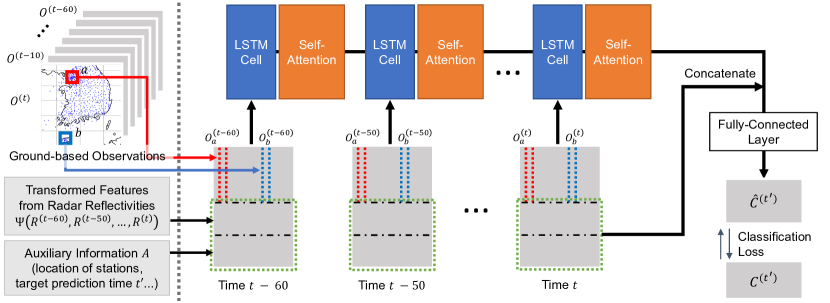
Figure 1: The overall inference process of ASOC+. Each ground-based observation snapshot is concatenated with (a) the pixel embeddings transformed from radar reflectivity images (e.g., by DeepRaNE [3]) and (b) auxiliary information. Then, the concatenated features are used as the input of a recurrent architecture that consists of LSTM cells and self-attention modules. Lastly, the final prediction results are determined based on the output of the recurrent architecture.

In this section, we present ASOC, a novel deep-learning model for precipitation nowcasting based on meteorological observations collected from multiple weather stations. We also discuss ASOC+, where ASOC is combined with a radar-image-based model for precipitation nowcasting.

IV-A Overview

In order to fully utilize multiple ground-based observations, we need to consider the following aspects:

• Temporal dynamics of observations: A sequence of ground-based observations over time are given as inputs, and temporal dynamics of them are useful for prediction.

• Contextual relationships between observations: Ground-based observations collected from different weather stations are related to each other, and the strength of relation between each pair, which is useful for prediction, depends on context, such as lead times, overall weather conditions, and distance between weather stations.

In order to capture the temporal dynamics of ground-based observations, we parameterize the function $\Phi$ in Problem 1 using a recurrent neural network (RNN), specifically LSTM [14]. Additionally, we use self-attention [15] to learn contextual relationships between pairs of ground weather stations. We provide a pictorial description of the overall architecture of ASOC+ in Figure 1, and we describe the architecture and the inference process in detail in the following subsections.

IV-B Exploiting temporal dynamics

Given consecutive snapshots of ground-based observations over time, capturing temporal dynamics of them is vital to precipitation nowcasting. Instead of processing the observations using a permutation-invariant model, which results in loss of temporal information, it is reasonable to use recurrent architectures for the parameterization and feed the inputs into the model in sequential order. We use LSTM [14], one of the most popular ones among such models. Note that, each LSTM cell processes inputs for one weather station at a time. Thus, inside each LSTM cell, the observations obtained from one station do not directly affect the outputs for the other stations.

IV-C Exploiting contextual relationships between observations

Instead of considering relation between observations inside the LSTM cells, we consider them separately in the self-attention blocks between LSTM cells. Specifically, among the hidden states and cell states of the LSTM, we only transform the hidden states using an attention mechanism while keeping the cell states as they are. For self-attention, we used an encoder layer of Transformer [15], which consists of a multi-head attention layer and a feed-forward network. In our experiments, we did not use layer normalization at all since the input ground-based observations contain scale-sensitive features, such as rainfall amount.

Input: (a) time of prediction $t$

(b) target time $t^{\prime}\in\{t+60,\cdots,t+360\}$

(c) snapshots of ground observations $O^{(t-60)}$, $\cdots$, $O^{(t)}$

(d) snapshots of radar reflectivities $R^{(t-60)}$, $\cdots$, $R^{(t)}$

(e) auxiliary information of all regions $\{A_{i}\}_{i\in I}$

(f) trained radar-image-based model $\Psi$ (spec., [3])

(g) trained parameters of ASOC+: $\mathbf{W}$, $\mathbf{b}$, and the parameters of LSTMCell and MultiHeadAttention

Output: Predicted probability distributions $\{\hat{C}_{i}^{(t)}\}_{i\in I}$

1

2$\tilde{R}$ $\leftarrow$ $\Psi(R^{(t-60)},\cdots,R^{(t)},t^{\prime}-t)$

3 $S_{h}$ $\leftarrow$ $\{\emptyset\}_{i\in I}$ // hidden state of LSTM

4 $S_{c}$ $\leftarrow$ $\{\emptyset\}_{i\in I}$ // cell state of LSTM

5 for $j\leftarrow t-60$ to $t$ by $10$ do

6       foreach $i\in I$ do

7             $X^{(j)}_{i}$ $\leftarrow$ $\text{{CONCATENATE}}(O^{(j)}_{i},\tilde{R}_{i},A_{i})$

8             $(S_{h,i},S_{c,i})$ $\leftarrow$ $\text{{LSTMCell}}(X^{(j)}_{i},S_{h,i},S_{c,i})$

9            

10      $\{S_{h,i}\}_{i\in I}$ $\leftarrow$ $\text{{MultiHeadAttention}}(\{S_{h,i}\}_{i\in I})$

11      

12foreach $i\in I$ do

13       $Y_{i}$ $\leftarrow$ $\text{{CONCATENATE}}(S_{h,i},\tilde{R}_{i},A_{i})$

14       $\hat{C}^{(t^{\prime})}_{i}$ $\leftarrow$ $\mathbf{W}{Y_{i}}+\mathbf{b}$

return $\{\hat{C}_{i}^{(t^{\prime})}\}_{i\in I}$

Algorithm 1 Inference step of ASOC+

IV-D Integration to image-based prediction models

In addition to ground-based observations, any extra information (e.g., radar reflectivity in each region) can be fed into our model. As auxiliary information, we use the location of each station and the lead time. Specifically, we use (a) a two-dimensional vector representing the location of each region, (b) a two-dimensional vector representing the observation date, (c) a two-dimensional vector representing the observation time, and (d) a six-dimensional one-hot vector for the lead time. Note that the last two vectors are the same for all regions. For each two-dimensional vector for location, we use the coordinates after min-max normalization. For the two-dimensional vectors for observation date and time, we perform min-max normalization and feed the result into the sine and cosine functions (see [21] for details of the positional encoding method). The vectors are all concatenated to the vector of ground-based observations at each weather station.

Moreover, output pixel embeddings of image-based precipitation nowcasting models can also be used as an additional input. While any existing image-based precipitation nowcasting model can be used for this purpose, we choose DeepRaNE [3], which is a state-of-the-art radar-image-based prediction model to be combined with ASOC. We call the combined model ASOC+. To sum up, for each region $x\in I$, the final input feature of ASOC+ for region $x$ and time $t$ is the concatenated vector of (a) the ground observation feature $O_{x}^{(t)}$, (b) the pixel embedding of the corresponding region obtained by DeepRaNE, and (c) the two-dimensional vector for representing the location of $x$, and (d) the ten-dimensional common auxiliary information vector. In ASOC, all vectors except for (b) are concatenated to be used as the input.

After obtaining the output of the LSTM part, ASOC and ASOC+ obtain the final output probability distribution $\{\hat{C}^{(t)}_{i}\}_{i\in I}$ for each region through an additional fully-connected layer. Together with the output of the LSTM part, the final input vector of the LSTM part are also fed into the last fully-connected layer. The pseudocode for the overall inference step of ASOC+ is provided in Algorithm 1.

IV-E Training method

For training ASOC+, we adapt the training protocol in [3]. Specifically, we split the training process into two steps: (a) pre-training with radar images and (b) fine-tuning with radar images and ground-based observations. During pre-training, we only consider the parameters of DeepRaNE and use the Earth-mover distance as the loss function to minimize the gap between the predicted probability distribution over $100$ radar reflectivity classes. Then, we fine-tune the whole model using the loss function proposed in [3], which is the negative average of approximated CSI scores defined as follows:

$$\mathcal{L}(C^{(t^{\prime})},\hat{C}^{(t^{\prime})})=-\frac{1}{2}\sum_{c\in\{\textsc{Heavy},\textsc{Rain}\}}\frac{\widetilde{\text{TP}}_{c}}{\widetilde{\text{TP}}_{c}+\widetilde{\text{FP}}_{c}+\widetilde{\text{FN}}_{c}},$$ (3)

where $\widetilde{\text{TP}}_{c}$, $\widetilde{\text{FP}}_{c}$, $\widetilde{\text{FN}}_{c}$ are differentiable approximations of the number of true positives, false positives, and false negatives for each precipitation class $c$. Refer to [3] for the details of the approximations and the pre-training step. When training ASOC, we perform only the fine-tuning step using ground-based observations.

V Experiments

TABLE II: Predictive performances on the test set. ASOC performs best overall among the methods that use only the ground-based observations as inputs. ASOC+ performs best overall among the methods that use ground-based observations and/or radar images as inputs. In each setting, the best score from the same input data is in bold.

Input Data		Ground-based Observations Only						Ground-based Observations and Radar Images
Precipitation level	Lead time	ASOC		LSTM		Persistence		ASOC+		DeepRaNE + Kriging		DeepRaNE only
		CSI	F1	CSI	F1	CSI	F1	CSI	F1	CSI	F1	CSI	F1
Heavy ($\geq$10mm/h)	$60$ minutes	0.262	0.415	0.296	0.457	0.259	0.412	0.444	0.615	0.316	0.480	0.390	0.562
	$120$ minutes	0.156	0.270	0.178	0.302	0.152	0.264	0.309	0.472	0.200	0.333	0.280	0.438
	$180$ minutes	0.120	0.215	0.127	0.225	0.102	0.185	0.218	0.357	0.158	0.273	0.210	0.348
	$240$ minutes	0.094	0.173	0.090	0.166	0.073	0.136	0.169	0.289	0.128	0.226	0.170	0.291
	$300$ minutes	0.079	0.147	0.064	0.121	0.057	0.108	0.141	0.247	0.108	0.195	0.135	0.238
	$360$ minutes	0.070	0.132	0.048	0.091	0.046	0.087	0.096	0.176	0.092	0.168	0.116	0.207
Rain ($\geq$1mm/h)	$60$ minutes	0.532	0.695	0.527	0.690	0.518	0.683	0.671	0.803	0.483	0.652	0.609	0.757
	$120$ minutes	0.430	0.602	0.408	0.580	0.396	0.568	0.548	0.708	0.409	0.581	0.501	0.667
	$180$ minutes	0.376	0.546	0.347	0.515	0.331	0.498	0.468	0.638	0.375	0.546	0.449	0.620
	$240$ minutes	0.334	0.501	0.306	0.468	0.288	0.447	0.428	0.599	0.339	0.507	0.411	0.583
	$300$ minutes	0.299	0.460	0.275	0.432	0.256	0.408	0.394	0.565	0.315	0.479	0.381	0.552
	$360$ minutes	0.270	0.425	0.250	0.401	0.231	0.375	0.359	0.529	0.294	0.454	0.354	0.523
Average		0.252	0.382	0.243	0.371	0.226	0.348	0.354	0.500	0.268	0.408	0.334	0.482

In this section, we review our experiments performed to answer the following questions:

1. Effectiveness of ASOC+ and ASOC: Is ASOC+ more accurate than baseline methods? How does ASOC perform compared to baseline methods relying only on ground-based observations?

2. Ablation Study: How much each ground-based meteorological feature contribute to the performance ASOC+? How does the self-attention block in ASOC and ASOC+ affect their overall accuracy?

3. Further Analysis in Heavy Rainfall Cases: How accurate is ASOC+ for heavy rainfall cases with precipitation intensity levels exceeding $30$ mm/hr on the test set?

V-A Experimental settings

V-A1 Machine

We performed all experiments on a server with 512GB of RAM and eight RTX 8000 GPUs, each of which has 48GB of GPU memory.

V-A2 Datasets

For radar data, we used radar reflectivity images around South Korea that were measured every ten minutes from 2014 to 2020. Each radar image is 1468 x 1468 in size and has a 1 km x 1 km resolution. For observations from ground weather stations, we used the data collected every 10 minutes from 2014 to 2020 from 714 automated weather stations (AWS) installed in South Korea. The meteorological features collected from ground weather stations are (a) 9 features related to wind direction and speed, (b) a feature related to one-minute average temperature, (c) a binary feature related to precipitation, (d) 4 features related to cumulative precipitation in 15 minutes, 1 hour, 12 hours, and 24 hours, (e) a feature related to relative humidity, and (6) 2 features related to barometric pressure.

V-A3 Baseline approaches

As baseline approaches that use ground-based observations and/or radar images, we used (a) DeepRaNE [3] and (b) DeepRaNE + Kriging. For the latter, we interpolated the ground-based observations to obtain grid-shaped data, using Kriging [13], and concatenated them to the input of DeepRaNE as additional channels. As baseline approaches that use only ground-based observations, we used (c) a vanilla LSTM model and (d) the persistence model. The LSTM model performs precipitation nowcasting based on the sequence of ground-based observations and the auxiliary information (spec., the location of the weather station, the observation date, the observation time, and the lead time), which are encoded as described in Section IV-D. Note that, compared to ASOC, the LSTM model uses all but radar images as its input. Also note that the LSTM model does not have the attention block, and thus once it is trained, it performs prediction independently for each region. The persistence model is a simple heuristic that uses the current precipitation class in each region as its prediction in the region regardless of lead times.

V-A4 Experimental setup

For DeepRaNE and its training process, we used the open-source implementation provided by the authors. For kriging, we used the PyKrige library. For the experimental setup, we mostly followed the protocol in [3]. For all experiments, we used the inputs from 2014 to 2018 for training, those in 2019 for validation, and those in 2020 for evaluation. In order to train models, we used the loss functions in Eq. (3) and the Adam [22] optimizer with a learning rate $2\times 10^{-5}$. When pre-training DeepRaNE, we set the batch size to 20 and the number of training steps to $50,000$. For the other training processes, we set the batch size to 24 and the number of steps to $35,000$. For every $1,000$ steps, we evaluated the model on the validation set and selected the trained model that performs best in the validation dataset. For DeepRaNE and the corresponding part of ASOC+, we set the number of initial hidden channels to $32$. For ASOC, we set the hidden dimension for LSTM cells to $64$ and the number of heads for the attention blocks to $4$.

V-A5 Evaluation metrics

For evaluation, we used the CSI and F1 scores for two precipitation classes, Heavy ($\geq$ 10mm/hour) and Rain ($\geq$ 1mm/hour), at each lead time (i.e,. 1 to 6 hours). Their formula is given in Eqs. (1) an (2). They have been used widely for precipitation nowcasting [4, 5, 3].

TABLE III: Ablation study results. The most crucial features among those in ground-based observations were cumulative precipitations, and removing the self-attention blocks from ASOC+ was harmful to the overall performance. Recall that removing the self-attention blocks from ASOC was also harmful, as shown in Table II. In each setting, the best score is in bold.

Precipitation level	Lead time	ASOC+		ASOC-A		ASOC-P		ASOC-W		ASOC-T		ASOC-D		ASOC-H		ASOC-B
		CSI	F1	CSI	F1	CSI	F1	CSI	F1	CSI	F1	CSI	F1	CSI	F1	CSI	F1
Heavy ($\geq$10mm/h)	$60$ minutes	0.444	0.615	0.464	0.634	0.399	0.571	0.406	0.578	0.317	0.481	0.297	0.458	0.380	0.550	0.408	0.579
	$120$ minutes	0.309	0.472	0.285	0.443	0.292	0.452	0.243	0.392	0.259	0.412	0.240	0.387	0.277	0.434	0.270	0.425
	$180$ minutes	0.218	0.357	0.218	0.358	0.207	0.343	0.186	0.313	0.205	0.340	0.202	0.336	0.213	0.351	0.196	0.328
	$240$ minutes	0.169	0.289	0.154	0.267	0.162	0.279	0.153	0.266	0.160	0.276	0.161	0.277	0.171	0.291	0.131	0.232
	$300$ minutes	0.141	0.247	0.125	0.222	0.124	0.221	0.120	0.214	0.131	0.231	0.138	0.242	0.132	0.233	0.136	0.239
	$360$ minutes	0.096	0.176	0.094	0.172	0.094	0.173	0.109	0.197	0.103	0.187	0.124	0.221	0.117	0.209	0.115	0.206
Rain ($\geq$1mm/h)	$60$ minutes	0.671	0.803	0.670	0.802	0.657	0.793	0.623	0.768	0.588	0.740	0.645	0.784	0.609	0.757	0.630	0.773
	$120$ minutes	0.548	0.708	0.550	0.710	0.549	0.709	0.516	0.681	0.517	0.682	0.520	0.684	0.523	0.687	0.526	0.690
	$180$ minutes	0.468	0.638	0.477	0.646	0.488	0.656	0.451	0.622	0.466	0.635	0.460	0.630	0.468	0.637	0.463	0.633
	$240$ minutes	0.428	0.599	0.425	0.596	0.440	0.611	0.413	0.585	0.421	0.593	0.414	0.585	0.426	0.598	0.391	0.562
	$300$ minutes	0.394	0.565	0.390	0.561	0.404	0.576	0.366	0.535	0.390	0.561	0.380	0.550	0.390	0.561	0.393	0.564
	$360$ minutes	0.359	0.529	0.365	0.535	0.371	0.541	0.336	0.503	0.361	0.530	0.356	0.525	0.362	0.531	0.364	0.533
Average		0.354	0.500	0.351	0.496	0.349	0.494	0.327	0.471	0.326	0.472	0.328	0.473	0.339	0.487	0.335	0.480

V-B Q1. Effectiveness of ASOC+ and ASOC

In order to demonstrate the effectiveness of ASOC+ and ASOC, we compared the performances of them and the aforementioned baseline approaches. The CSI and F1 scores are provided in Table II. First, among the approaches that use only ground-based observations as the input, ASOC performed significantly better than the others, demonstrating the effectiveness of our proposed idea (i.e., using the attention blocks between LSTM cells). In addition, among the approaches that use ground-based observations and/or radar images, ASOC+ performed best overall, achieving the $5.7\%$ better CSI scores on average than the others. Especially, for the precipitation class Rain, ASOC+ performs best at all lead times. Notably, the performance of DeepRaNE + Kriging was even worse than DeepRaNE, while it outperformed all methods that use only ground-based observations as inputs. One potential reason is interpolation error induced by Kriging.

V-C Q2. Ablation Study

We investigated the effect of the features in the ground-based observations and the self-attention block on the model’s performance. To compare the performance, we compared ASOC+ with the following variants, each of which was trained following the same training protocol of ASOC+:

1. ASOC+: the proposed method that uses all ground-based features.

2. ASOC-A: a variant without self-attention blocks in the architecture.

3. ASOC-W: a variant that uses only those related to wind direction and speed among ground-based features.

4. ASOC-T: a variant that uses only those related to average temperature among ground-based features.

5. ASOC-P: a variant that uses only those related to cumulative precipitation among ground-based features.

6. ASOC-D: a variant that uses only that related to precipitation detection among ground-based features.

7. ASOC-H: a variant that uses only that related to relative humidity among ground-based features.

8. ASOC-B: a variant that uses those related to barometric pressure among ground-based features.

We measured the CSI and F1 scores for each method, which are reported in Table III. For the precipitation class Heavy, ASOC+ achieved the best CSI and F1 scores on average, followed by ASOC-A and ASOC-P. Especially, ASOC+ achieved the best CSI scores at all lead times except 1 and 3 hours. While ASOC+ was slightly outperformed by ASOC-P at most lead times for the precipitation class Rain, ASOC+ still performed best overall when considering all $12$ settings, followed by ASOC-A and ASOC-P. That is, removing the self-attention blocks from ASOC+ tended to be harmful, as removing them from ASOC was (compare ASOC and LSTM in Table II). From the results, we also observed that, overall, the ground-based features for cumulative precipitation contributed most to the performance of ASOC+, followed by the those for relative humidity and barometric pressure.

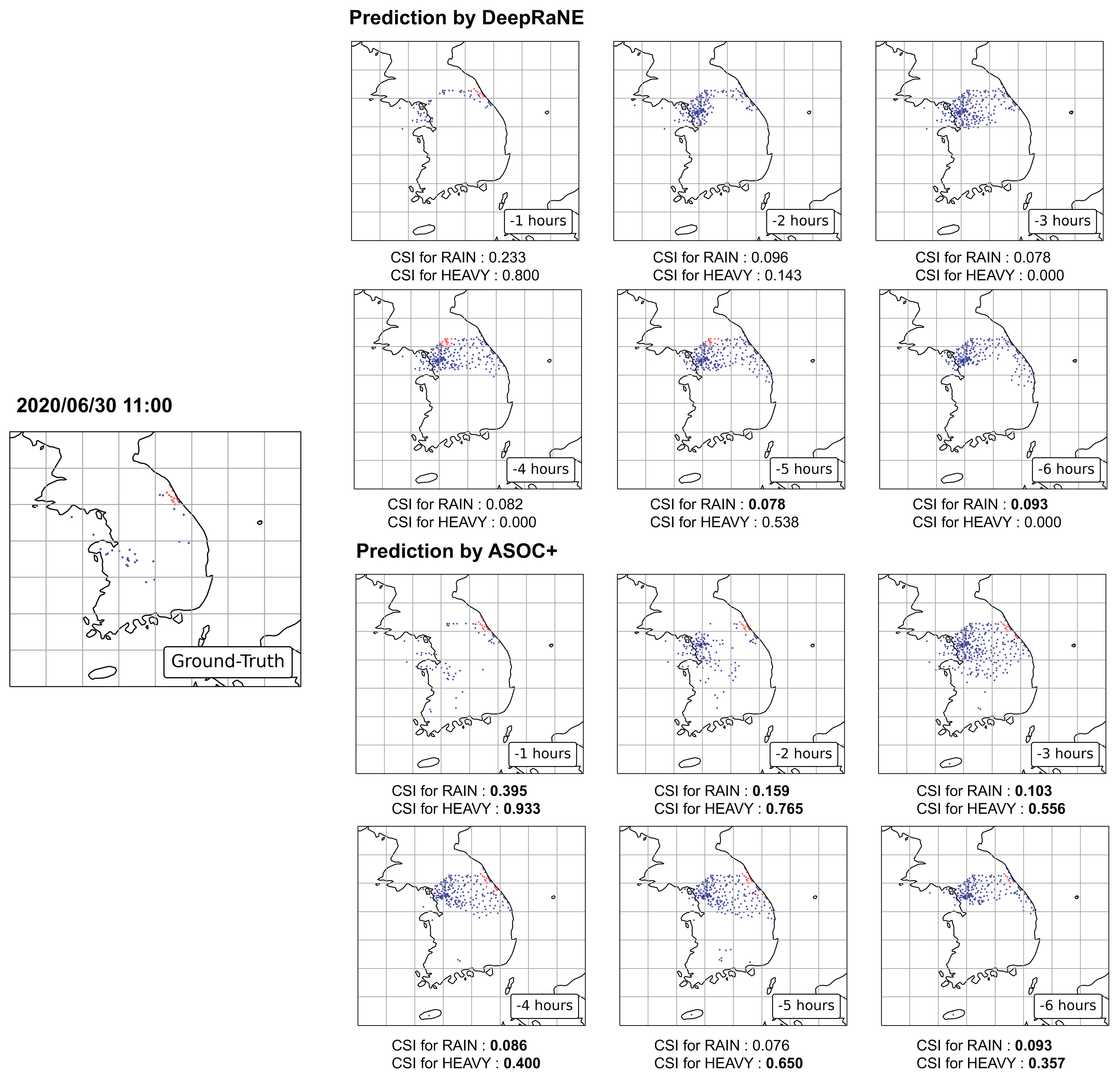
Figure 2: Comparison of predictions made by ASOC+ and DeepRaNE for heavy rainfall cases (June 30, 2020 at 11 am). The Heavy ($\geq 10$ mm/hr) cases and Light ($1$ - $10$ mm/hr) cases are marked in red and blue, respectively. The largest figure on the left shows the ground-truth precipitation classes, and the others showed prediction results (spec., most probable classes) at different lead times. The CSI scores at each lead time are provided below the figures. Between the two CSI scores obtained by the two compared methods for each precipitation level at each lead time, the higher one is in bold. Note that the prediction results from the both methods become closer to the ground truth as the lead time reduces. Note that, although DeepRaNE fails to predict the locations of Heavy cases when the lead time is greater than $2$ hours, ASOC+ predicts the locations quite accurately even when the lead time is $6$ hours.

V-D Q3. Further Analysis in Heavy Rainfall Cases

We further analyzed the performance of ASOC+ in $425$ cases in the test set where a precipitation intensity rate of 30 mm/hr or more was observed at one or more regions. On average, the CSI score for the precipitation classes Heavy ($\geq 10$ mm/hr) and Rain ($\geq 1$ mm/hr) were 0.234 and 0.465, respectively. Specifically, compared to DeepRaNE, ASOC+ achieved 18.7% (49.3% at a 5-hr lead time) better CSI scores on average for Heavy and 19.6% (49.1% at a 5-hr lead time) better F1 scores on average. Figure 2 shows the detailed predictions provided by ASOC+ and DeepRaNE at different lead times in one of the heavy-rainfall cases.

VI Conclusion

In this work, we proposed ASOC, a novel attentive and recurrent model for precipitation nowcasting using ground-based observations. We designed ASOC to effectively utilize meteorological observations collected from multiple ground weather stations by allowing it to capture temporal dynamics of the observations and the attentive relationships between them. In addition, we proposed ASOC+, where ASOC is combined with DeepRaNE, which is a state-of-the-art radar-image-based model. Using ground-based observations (from $714$ ground weather stations) radar reflectivities collected around South Korea for seven years, we demonstrated the effectiveness of ASOC and ASOC+. Specifically, we showed that ASOC+ improved the CSI score of predicting heavy (at least 10 mm/hr) and light (at least 1 mm/hr) rainfall events at 1-6 hr lead times by 5.7%, compared to DeepRaNE. In addition, we measured the contribution of various features in ground-based observations to the performance of ASOC+ and conducted a case study to further analyze the prediction results provided by ASOC+. For reproducibility, we made the source code used in the paper publicly available at https://github.com/jihoonko/ASOC.

References

- [1] X. Shi, Z. Chen, H. Wang, D.-Y. Yeung, W.-K. Wong, and W.-c. Woo, “Convolutional lstm network: A machine learning approach for precipitation nowcasting,” in NIPS, 2015.
- [2] X. Shi, Z. Gao, L. Lausen, H. Wang, D.-Y. Yeung, W.-k. Wong, and W.-c. Woo, “Deep learning for precipitation nowcasting: A benchmark and a new model,” in NIPS, 2017.
- [3] J. Ko, K. Lee, H. Hwang, S.-G. Oh, S.-W. Son, and K. Shin, “Effective training strategies for deep-learning-based precipitation nowcasting and estimation,” Computers & Geosciences, vol. 161, p. 105072, 2022.
- [4] S. Agrawal, L. Barrington, C. Bromberg, J. Burge, C. Gazen, and J. Hickey, “Machine learning for precipitation nowcasting from radar images,” arXiv preprint arXiv:1912.12132, 2019.
- [5] C. K. Sønderby, L. Espeholt, J. Heek, M. Dehghani, A. Oliver, T. Salimans, S. Agrawal, J. Hickey, and N. Kalchbrenner, “Metnet: A neural weather model for precipitation forecasting,” arXiv preprint arXiv:2003.12140, 2020.
- [6] V. Lebedev, V. Ivashkin, I. Rudenko, A. Ganshin, A. Molchanov, S. Ovcharenko, R. Grokhovetskiy, I. Bushmarinov, and D. Solomentsev, “Precipitation nowcasting with satellite imagery,” in KDD, 2019, pp. 2680–2688.
- [7] F. Schmid, Y. Wang, and A. Harou, “Nowcasting guidelines–a summary,” Bulletin nº, vol. 68, p. 2, 2019.
- [8] J. W. Wilson, E. E. Ebert, T. R. Saxen, R. D. Roberts, C. K. Mueller, M. Sleigh, C. E. Pierce, and A. Seed, “Sydney 2000 forecast demonstration project: convective storm nowcasting,” Weather and forecasting, vol. 19, no. 1, pp. 131–150, 2004.
- [9] L. Espeholt, S. Agrawal, C. Sønderby, M. Kumar, J. Heek, C. Bromberg, C. Gazen, J. Hickey, A. Bell, and N. Kalchbrenner, “Skillful twelve hour precipitation forecasts using large context neural networks,” arXiv preprint arXiv:2111.07470, 2021.
- [10] S. G. Benjamin, S. S. Weygandt, J. M. Brown, M. Hu, C. R. Alexander, T. G. Smirnova, J. B. Olson, E. P. James, D. C. Dowell, G. A. Grell et al., “A north american hourly assimilation and model forecast cycle: The rapid refresh,” Monthly Weather Review, vol. 144, no. 4, pp. 1669–1694, 2016.
- [11] O. Ronneberger, P. Fischer, and T. Brox, “U-net: Convolutional networks for biomedical image segmentation,” in MICCAI, 2015, pp. 234–241.
- [12] D. Shepard, “A two-dimensional interpolation function for irregularly-spaced data,” in ACM National Conference, 1968, pp. 517–524.
- [13] G. Metheron, “Theory of regionalized variables and its applications,” Les Cahiers de Morphologie Mathematique, vol. 5, p. 211, 1971.
- [14] S. Hochreiter and J. Schmidhuber, “Long short-term memory,” Neural computation, vol. 9, no. 8, pp. 1735–1780, 1997.
- [15] A. Vaswani, N. Shazeer, N. Parmar, J. Uszkoreit, L. Jones, A. N. Gomez, Ł. Kaiser, and I. Polosukhin, “Attention is all you need,” in NIPS, 2017.
- [16] S. Ravuri, K. Lenc, M. Willson, D. Kangin, R. Lam, P. Mirowski, M. Fitzsimons, M. Athanassiadou, S. Kashem, S. Madge et al., “Skilful precipitation nowcasting using deep generative models of radar,” Nature, vol. 597, no. 7878, pp. 672–677, 2021.
- [17] M. Mirza and S. Osindero, “Conditional generative adversarial nets,” arXiv preprint arXiv:1411.1784, 2014.
- [18] N. Ballas, L. Yao, C. Pal, and A. C. Courville, “Delving deeper into convolutional networks for learning video representations.” in ICLR, 2016.
- [19] S. Seo, A. Mohegh, G. Ban-Weiss, and Y. Liu, “Automatically inferring data quality for spatiotemporal forecasting,” in ICLR, 2018.
- [20] C. Wang, P. Wang, D. Wang, J. Hou, and B. Xue, “Nowcasting multicell short-term intense precipitation using graph models and random forests,” Monthly Weather Review, 2020.
- [21] G. Petneházi, “Recurrent neural networks for time series forecasting,” arXiv preprint arXiv:1901.00069, 2019.
- [22] D. P. Kingma and J. Ba, “Adam: A method for stochastic optimization,” in ICLR, 2015.