Decentralized Stochastic Bilevel Optimization with Improved per-Iteration Complexity

Abstract

Bilevel optimization recently has received tremendous attention due to its great success in solving important machine learning problems like meta learning, reinforcement learning, and hyperparameter optimization. Extending single-agent training on bilevel problems to the decentralized setting is a natural generalization, and there has been a flurry of work studying decentralized bilevel optimization algorithms. However, it remains unknown how to design the distributed algorithm with sample complexity and convergence rate comparable to SGD for stochastic optimization, and at the same time without directly computing the exact Hessian or Jacobian matrices. In this paper we propose such an algorithm. More specifically, we propose a novel decentralized stochastic bilevel optimization (DSBO) algorithm that only requires first order stochastic oracle, Hessian-vector product and Jacobian-vector product oracle. The sample complexity of our algorithm matches the currently best known results for DSBO, while our algorithm does not require estimating the full Hessian and Jacobian matrices, thereby possessing to improved per-iteration complexity.

1 Introduction

Many machines learning problems can be formulated as a bilevel optimization problem of the form,

$$\min_{x\in\mathbb{R}^{p}}\quad\Phi(x)=f(x,y^{*}(x))$$ (1)

$$\text{s.t.}\quad y^{*}(x)=\operatorname*{arg\,min}_{y\in\mathbb{R}^{q}}g(x,y),$$

where we minimize the upper level function $f$ with respect to $x$ subject to the constraint that $y^{*}(x)$ is the minimizer of the lower level function. Its applications can range from classical optimization problems like compositional optimization (Chen et al., 2021) to modern machine learning problems such as reinforcement learning (Hong et al., 2020), meta learning (Snell et al., 2017; Bertinetto et al., 2018; Rajeswaran et al., 2019; Ji et al., 2020), hyperparameter optimization (Pedregosa, 2016; Franceschi et al., 2018), etc. State-of-the-art bilevel optimization algorithms with non-asymptotic analyses include BSA (Ghadimi & Wang, 2018), TTSA (Hong et al., 2020), StocBiO (Ji et al., 2020), ALSET (Chen et al., 2021), to name a few.

Decentralized bilevel optimization aims at solving bilevel problems in a decentralized setting, which provides additional benefits such as faster convergence, data privacy preservation and robustness to low network bandwidth compared to the centralized setting and the single-agent training (Lian et al., 2017). For example, decentralized meta learning, which is a special case of decentralized bilevel optimization, arise naturally in the context of medical data analysis in the context of protecting patient privacy; see, for example, Altae-Tran et al. (2017); Zhang et al. (2019); Kayaalp et al. (2022). Motivated by such applications, the works of Lu et al. (2022); Chen et al. (2022b); Yang et al. (2022); Gao et al. (2022) proposed and analyzed various decentralized stochastic bilevel optimization (DSBO) algorithms.

From a mathematical perspective, DSBO aims at solving the following problem in a distributed setting:

$$\min_{x\in\mathbb{R}^{p}}\quad\Phi(x)=\frac{1}{n}\sum_{i=1}^{n}f_{i}(x,y^{*}(x))$$ (2)

$$\text{s.t.}\quad y^{*}(x)=\operatorname*{arg\,min}_{y\in\mathbb{R}^{q}}g(x,y):=\frac{1}{n}\sum_{i=1}^{n}g_{i}(x,y),$$

where $x\in\mathbb{R}^{p},y\in\mathbb{R}^{q}$. $f_{i}$ is possibly nonconvex and $g_{i}$ is strongly convex in $y$. Here $n$ denotes the number of agents, and agent $i$ only has access to stochastic oracles of $f_{i},\ g_{i}$. The local objectives $f_{i}$ and $g_{i}$ are defined as:

$$f_{i}(x,y) =\mathbb{E}_{\phi\sim\mathcal{D}_{f_{i}}}\left[F(x,y;\phi)\right],$$

$$g_{i}(x,y) =\mathbb{E}_{\xi\sim\mathcal{D}_{g_{i}}}\left[G(x,y;\xi)\right].$$

$\mathcal{D}_{f_{i}}$ and $\mathcal{D}_{g_{i}}$ represent the data distributions used to generate the objectives for agent $i$, and each agent only has access to $f_{i}$ and $g_{i}$. In practice we can replace the expectation by empirical loss, and then use samples to approximate the gradients in the updates. Existing works on DSBO require computing the full Hessian (or Jacobian) matrices in the hypergradient estimation, whose per-iteration complexity is $\mathcal{O}(q^{2})$ (or $\mathcal{O}(pq)$). In problems like hyperparameter estimation, the lower level corresponds to learning the parameters of a model. When considering modern overparametrized models, the order of $q$ is hence extremely large. Hence, to reduce the per-iteration complexity, it is of great interest to have each iteration based only on Hessian-vector (or Jacobian-vector) products, whose complexity is $\mathcal{O}(q)$ (or $\mathcal{O}(p)$); see, for example, Pearlmutter (1994).

1.1 Our contributions

Our contributions in this work are as follows.

• We propose a novel method to estimate the global hypergradient. Our method estimates the product of the inverse of the Hessian and vectors directly, without computing the full Hessian or Jacobian matrices, and thus improves the previous overall (both computational and communication) complexity on hypergradient estimation from $\mathcal{O}(Nq^{2})$ to $\mathcal{O}(Nq)$, where $N$ is the total steps of the hypergradient estimation subroutine.

• We design a DSBO algorithm (see Algorithm 3), and in Theorem 3.3 and Corollary 3.4 we show the sample complexity is of order $\mathcal{O}(\epsilon^{-2}\log\frac{1}{\epsilon})$, which matches the currently well-known results of the single-agent bilevel optimization (Chen et al., 2021). Our proof relies on weaker assumptions comparing to Yang et al. (2022), and is based on carefully combining moving average stochastic gradient estimation analyses with the decentralized bilevel algorithm analyses.

• We conduct experiments on several machine learning problems. Our numerical results show the efficiency of our algorithm in both the synthetic and the real-world problems. Moreover, since our algorithm does not store the full Hessian or Jacobian matrices, both the space complexity and the communication complexity are improved comparing to Chen et al. (2022b); Yang et al. (2022).

1.2 Related work

Bilevel optimization. Different from classical constrained optimization, bilevel optimization restricts certain variables to be the minimizer of the lower level function, which is more applicable in modern machine learning problems like meta learning (Snell et al., 2017; Bertinetto et al., 2018; Rajeswaran et al., 2019) and hyperparameter optimization (Pedregosa, 2016; Franceschi et al., 2018). In recent years, Ghadimi & Wang (2018) gave the first non-asymptotic analysis of the bilevel stochastic approximation methods, which attracted much attention to study more efficient bilevel optimization algorithms including AID-based (Domke, 2012; Pedregosa, 2016; Gould et al., 2016; Ghadimi & Wang, 2018; Grazzi et al., 2020; Ji et al., 2021), ITD-based (Domke, 2012; Maclaurin et al., 2015; Franceschi et al., 2018; Grazzi et al., 2020; Ji et al., 2021), and Neumann series-based (Chen et al., 2021; Hong et al., 2020; Ji et al., 2021) methods. These methods only require access to first order stochastic oracles and matrix-vector product (Hessian-vector and Jacobian-vector) oracles, which demonstrate great potential in solving bilevel optimization problems and achieve $\tilde{\mathcal{O}}(\epsilon^{-2})$ sample complexity (Chen et al., 2021; Arbel & Mairal, 2021) that matches the result of SGD for single level stochastic optimization ignoring the log factors. Moreover, under stronger assumptions and variance reduction techniques, better complexity bounds are obtained (Guo et al., 2021; Khanduri et al., 2021; Yang et al., 2021; Chen et al., 2022a).

Decentralized optimization. Extending optimization algorithms from a single-agent setting to a multi-agent setting has been studied extensively in recent years thanks to the modern parallel computing. Decentralized optimization, which does not require a central node, serves as an important part of distributed optimization. Because of data heterogeneity and the absence of a central node, decentralized optimization is more challenging and each node communicates with neighbors to exchange information and solve a finite-sum optimization problem. Under certain scenarios, decentralized algorithms are more preferable comparing to centralized ones since the former preserve data privacy (Ram et al., 2009; Yan et al., 2012; Wu et al., 2017; Koloskova et al., 2020) and have been proved useful when the network bandwidth is low (Lian et al., 2017).

Decentralized stochastic bilevel optimization. To make bilevel optimization applicable in parallel computing, recent work started to focus on distributed stochastic bilevel optimization. FEDNEST (Tarzanagh et al., 2022) and FedBiO (Li et al., 2022) impose federated learning, which is essentially a centralized setting, on stochastic bilevel optimization. Existing work on DSBO can be classified to two categories: global DSBO and personalized DSBO. Problem (2) that we consider in this paper is a global DSBO, where both lower-level and upper-level functions are not directly accessible to any local agent. Other works on global DSBO include Chen et al. (2022b); Yang et al. (2022); Gao et al. (2022). The personalized DSBO (Lu et al., 2022) replaces $y^{*}(x)$ by the local one $y_{i}^{*}(x)=\operatorname*{arg\,min}_{y\in\mathbb{R}^{q}}g_{i}(x,y)$ in (2), which leads to

$$\min_{x\in\mathbb{R}^{p}}\quad\Phi(x)=\frac{1}{n}\sum_{i=1}^{n}f_{i}(x,y_{i}^{*}(x))$$ (3)

$$\text{s.t.}\quad y_{i}^{*}(x)=\operatorname*{arg\,min}_{y\in\mathbb{R}^{q}}g_{i}(x,y),i=1,\ldots,n.$$

To solve global DSBO (2), Chen et al. (2022b) proposes a JHIP oracle to estimate the Jacobian-Hessian-inverse product while Yang et al. (2022) introduces a Hessian-inverse estimation subroutine based on Neumann series approach which can be dated back to Ghadimi & Wang (2018). However, they both require computing the full Jacobian or Hessian matrices, which is extremely time-consuming when $q$ is large. In comparison, computing a Hessian-vector or Jacobian-vector product is more efficient in large-scale machine learning problems (Bottou et al., 2018), and is commonly used in vanilla bilevel optimization (Ghadimi & Wang, 2018; Ji et al., 2021; Chen et al., 2021) to avoid computing the Hessian inverse. In personalized DSBO (3), local computation is sufficient to approximate $\nabla f_{i}(x,y_{i}^{*}(x))$, and thus does not require computing the Hessian or Jacobian matrices and single-agent bilevel optimization methods can be directly incorporated in the distributed regime. In our paper we propose a novel algorithm that estimates the global hypergradient using only first-order oracle and matrix-vector products oracle. Based on this we further design our algorithm for solving DSBO that does not require to compute the full Jacobian or Hessian matrices. We summarize the results of aforementioned works and our results in Table 1.

Notation. We denote by $\nabla f(x,y)$ and $\nabla^{2}f(x,y)$ the gradient and Hessian matrix of $f$, respectively. We use $\nabla_{x}f(x,y)$ and $\nabla_{y}f(x,y)$ to represent the gradients of $f$ with respect to $x$ and $y$, respectively. Denote by $\nabla_{xy}^{2}f(x,y)\in\mathbb{R}^{p\times q}$ the Jacobian matrix of $f$ and $\nabla_{y}^{2}f(x,y)$ the Hessian matrix of $f$ with respect to $y$. $\|\cdot\|$ denotes the $\ell_{2}$ norm for vectors and Frobenius norm for matrices, unless specified. $\mathbf{1}_{n}$ is the all one vector in $\mathbb{R}^{n}$, and $J_{n}=\mathbf{1}_{n}\mathbf{1}_{n}^{\top}$ is the $n\times n$ all one matrix. We use uppercase letters to represent the matrix that collecting all the variables (corresponding lowercase) as columns. For example $X_{k}=\left(x_{1,k},...,x_{n,k}\right),\ Y_{k}^{(t)}=\left(y_{1,k}^{(t)},...,y_{n,k}^{(t)}\right)$. We add an overbar to a letter to denote the average over all nodes. For example, $\bar{x}_{k}=\frac{1}{n}\sum_{i=1}^{n}x_{i,k},\ \bar{y}_{k}^{(t)}=\frac{1}{n}\sum_{i=1}^{n}y_{i,k}^{(t)}$.

Table 1: We compare our Algorithm 3 (MA-DSBO) with existing distributed bilevel optimization algorithms: FEDNEST (Tarzanagh et al., 2022), SPDB (Lu et al., 2022), DSBO-JHIP (Chen et al., 2022b), and GBDSBO (Yang et al., 2022). The problem types include Federated Bilevel Optimization (FBO), Personalized-Decentralized Stochastic Bilevel Optimization (P-DSBO), and Global-Decentralized Stochastic Bilevel Optimization (G-DSBO). In the table we define $d=\max\left(p,q\right)$. ’Computation’ (See Section C.3 for details) and ’Samples’ represent the computational and sample complexity of finding an $\epsilon$-stationary point, respectively. $\tilde{\mathcal{O}}$ hides the $\log(\frac{1}{\epsilon})$ factor. ’Jacobian’ refers to whether the algorithm requires computing full Hessian or Jacobian matrix. ’Mini-batch’ refers to whether the algorithm requires their batch size depending on $\epsilon^{-1}$.

Algorithm	Problem	Computation	Samples	Jacobian	Mini-batch	Network
FEDNEST	FBO	$\tilde{\mathcal{O}}(d\epsilon^{-2})$	$\tilde{\mathcal{O}}(\epsilon^{-2})$	No	No	Centralized
SPDB	P-DSBO	$\tilde{\mathcal{O}}(dn^{-1}\epsilon^{-2})$	$\tilde{\mathcal{O}}(n^{-1}\epsilon^{-2})$	No	Yes	Decentralized
DSBO-JHIP	G-DSBO	$\tilde{\mathcal{O}}(pq\epsilon^{-3})$	$\tilde{\mathcal{O}}(\epsilon^{-3})$	Yes	No	Decentralized
GBDSBO	G-DSBO	$\mathcal{O}((q^{2}\log(\frac{1}{\epsilon})+pq)n^{-1}\epsilon^{-2})$	$\tilde{\mathcal{O}}(n^{-1}\epsilon^{-2})$	Yes	No	Decentralized
MA-DSBO	G-DSBO	$\tilde{\mathcal{O}}(d\epsilon^{-2})$	$\tilde{\mathcal{O}}(\epsilon^{-2})$	No	No	Decentralized

2 Preliminaries

The following assumptions are used throughout this paper. They are standard assumptions that are made in the literature on bilevel optimization (Ghadimi & Wang, 2018; Hong et al., 2020; Chen et al., 2021; Ji et al., 2021; Huang et al., 2022) and decentralized optimization (Qu & Li, 2017; Nedic et al., 2017; Lian et al., 2017; Tang et al., 2018).

Assumption 2.1 (Smoothness).

There exist positive constants $\mu_{g}$, $L_{f,0}$, $L_{f,1}$, $L_{g,1}$, $L_{g,2}$ such that for any $i$, functions $f_{i}$, $\nabla f_{i}$, $\nabla g_{i}$, $\nabla^{2}g_{i}$ are $L_{f,0}$, $L_{f,1}$, $L_{g,1}$, $L_{g,2}$ Lipschitz continuous respectively, and function $g_{i}$ is $\mu_{g}$-strongly convex in $y$.

Assumption 2.2 (Network topology).

The weight matrix $W=(w_{ij})\in\mathbb{R}^{n\times n}$ is symmetric and doubly stochastic, i.e.:

$$W=W^{\top},\quad W\mathbf{1_{n}}=\mathbf{1_{n}},\quad w_{ij}\geq 0,\forall i,j,$$

and its eigenvalues satisfy $1=\lambda_{1}>\lambda_{2}\geq...\geq\lambda_{n}$ and $\rho:=\max\{|\lambda_{2}|,|\lambda_{n}|\}<1$.

The weight matrix given in Assumption 2.2 characterizes the network topology by setting the weight parameter between agent $i$ and agent $j$ to be $w_{ij}$. The condition $\rho<1$ is termed as ’spectral gap’ (Lian et al., 2017), and is used in distributed optimization to ensure the decay of the consensus error, i.e., $\frac{\mathbb{E}\left[\|X_{k}-\bar{x}_{k}\mathbf{1}^{\top}_{n}\|^{2}\right]}{n}$, among the agents, which eventually guarantees the consensus among agents.

Assumption 2.3 (Gradient heterogeneity).

There exists a constant $\delta\geq 0$ such that for all $1\leq i\leq n,x\in\mathbb{R}^{p},y\in\mathbb{R}^{q},$

$$\|\nabla_{y}g_{i}(x,y)-\frac{1}{n}\sum_{l=1}^{n}\nabla_{y}g_{l}(x,y)\|\leq\delta.$$

The above assumption is commonly used in distributed optimization literature (see, e.g., Lian et al. (2017)), and it indicates the level of similarity between the local gradient and the global gradient. Moreover, it is weaker than the Assumption 3.4 (iv) of Yang et al. (2022) which assumes that $\nabla_{y}g_{i}(x,y;\xi)$ has a bounded second moment. This is because the bounded second moment implies the boundedness of $\nabla_{y}g(x,y)$, as we have

$$\|\nabla_{y}g(x,y)\|^{2}$$

$$\leq \mathbb{E}\left[\|\nabla_{y}g(x,y)-\nabla_{y}g(x,y;\xi)\|^{2}\right]+\|\nabla_{y}g(x,y)\|^{2}$$

$$= \mathbb{E}\left[\|\nabla_{y}g(x,y;\xi)\|^{2}\right]\text{ -- uniformly bounded,}$$

where the equality holds since we have $\mathbb{E}\left[\|X\|^{2}\right]=\mathbb{E}\left[\|X-\mathbb{E}\left[X\right]\|^{2}\right]+\|\mathbb{E}\left[X\right]\|^{2}$ for any random vector $X$. It directly gives the inequality in Assumption 2.3. However Assumption 2.3 does not imply the boundedness of $\nabla_{y}g(x,y)$ (e.g., $g_{i}(x,y)=y^{\top}y$ for all $i$ satisfies Assumption 2.3 but does not have bounded gradient.)

Assumption 2.4 (Bounded variance).

The stochastic derivatives, $\nabla f_{i}(x,y;\phi)$, $\nabla g_{i}(x,y;\xi)$, and $\nabla^{2}g_{i}(x,y;\xi)$, are unbiased with bounded variances $\sigma_{f}^{2}$, $\sigma_{g,1}^{2}$, $\sigma_{g,2}^{2}$, respectively.

Note that we do not make any assumptions on whether the data distributions are heterogeneous or identically distributed.

3 DSBO Algorithm with Improved Per-Iteration Complexity

We start with following standard result in the bilevel optimization literature (Ghadimi & Wang, 2018; Hong et al., 2020; Ji et al., 2020; Chen et al., 2021) that gives a closed form expression of the hypergradient $\nabla\Phi(x)$, making gradient-based bilevel optimization tractable.

Lemma 3.1.

Suppose Assumption 2.1 holds. The hypergradient $\nabla\Phi(x)$ of (2) takes the form:

$$\nabla\Phi(x)= \frac{1}{n}\left(\sum_{i=1}^{n}\nabla_{x}f_{i}(\tilde{x})\right)$$ (4)

$$-\nabla_{xy}^{2}g(\tilde{x})\left(\nabla_{y}^{2}g(\tilde{x})\right)^{-1}\left[\frac{1}{n}\left(\sum_{i=1}^{n}\nabla_{y}f_{i}(\tilde{x})\right)\right],$$

where $\tilde{x}=(x,y^{*}(x))$.

We also include smoothness properties of $\nabla\Phi(x)$ and $y^{*}(x)$ in Section B in the appendix.

3.1 Main challenge

As discussed in Chen et al. (2022b) and Yang et al. (2022), the main challenge in designing DSBO algorithms is to estimate the global hypergradient. This is challenging because of the data heterogeneity across agents, which leads to

$$\begin{aligned} &\nabla_{xy}^{2}g(x,y^{*}(x))\left(\nabla_{y}^{2}g(x,y^{*}(x))\right)^{-1}\\ \neq&\frac{1}{n}\sum_{i=1}^{n}\nabla_{xy}^{2}g_{i}(x,y_{i}^{*}(x))\left(\nabla_{y}^{2}g_{i}(x,y_{i}^{*}(x))\right)^{-1},\end{aligned}$$ (5)

where $y_{i}^{*}(x)=\operatorname*{arg\,min}_{y\in\mathbb{R}^{q}}g_{i}(x,y)$. This shows that simply averaging the local hypergradients does not give a good approximation to the global hypergradient. A decentralized approach should be designed to estimate the global hypergradient $\nabla\Phi(x)$.

To this end, the JHIP oracle in Chen et al. (2022b) manages to estimate

$$\left(\sum_{i=1}^{n}\nabla_{xy}^{2}g_{i}(x,y^{*}(x))\right)\left(\sum_{i=1}^{n}\nabla_{y}^{2}g_{i}(x,y^{*}(x))\right)^{-1}$$

using decentralized optimization approach, and Yang et al. (2022) proposed to estimate the global Hessian-inverse, i.e.,

$$\left(\sum_{i=1}^{n}\nabla_{y}^{2}g_{i}(x,y^{*}(x))\right)^{-1}$$

via a Neumann series based approach. Instead of focusing on full matrices computation, we consider approximating

$$z=\left(\sum_{i=1}^{n}\nabla_{y}^{2}g_{i}(x,y^{*}(x))\right)^{-1}\left(\sum_{i=1}^{n}\nabla_{y}f_{i}(x,y^{*}(x))\right).$$ (6)

According to (4), the global hypergradient is given by

$$\nabla\Phi(x)=\frac{1}{n}\sum_{i=1}^{n}(\nabla_{x}f_{i}(x,y^{*}(x))-\nabla_{xy}^{2}g_{i}(x,y^{*}(x))z).$$ (7)

From the above expression we know that as long as node $i$ can have a good estimate of $\nabla_{x}f_{i}(x,y^{*}(x))$ and $\nabla_{xy}^{2}g_{i}(x,y^{*}(x))z$, then on average the update will be a good approximation to the global hypergradient. More importantly, the process of estimating $z$ can avoid computing the full Hessian or Jacobian matrices.

3.2 Hessian-Inverse-Gradient-Product oracle

Solving (6) is essentially a decentralized optimization with a strongly convex quadratic objective function. Suppose each agent only has access to $H_{i}\in\mathbb{S}_{++}^{q\times q}$ and $b_{i}\in\mathbb{R}^{q}$, and all the agents collectively solve for

$$\sum_{i=1}^{n}H_{i}z=\sum_{i=1}^{n}b_{i},\ \text{or }z=\left(\sum_{i=1}^{n}H_{i}\right)^{-1}\left(\sum_{i=1}^{n}b_{i}\right).$$ (8)

From an optimization perspective, the above expression is the optimality condition of:

$$\min_{z\in\mathbb{R}^{q}}\frac{1}{n}\sum_{i=1}^{n}h_{i}(z),\ \text{where }h_{i}(z)=\frac{1}{2}z^{\top}H_{i}z-b_{i}^{\top}z.$$ (9)

Hence we can design a decentralized algorithm to solve for $z$ without the presence of a central server. Based on this observation and (7), we present our Hessian-Inverse-Gradient Product oracle in Algorithm 1.

Algorithm 1 Hessian-Inverse-Gradient Product oracle

1:  Input: $(H_{i,t}^{(k)},b_{i,t}^{(k)})$, for $0\leq t\leq N$ accessible only to agent $i$. Stepsize $\gamma$, iteration number $N$, $d_{i,0}^{(k)}=-b_{i,0}^{(k)},\ s_{i,0}^{(k)}=-b_{i,0}^{(k)},\ \text{and }z_{i,0}^{(k)}=0$

2:  for $t=0,1,...,N-1$ do

3:     for $i=1,...,n$ do

4:        $z_{i,t+1}^{(k)}=\sum_{j=1}^{n}w_{ij}z_{j,t}^{(k)}-\gamma d_{i,t}^{(k)}$,

5:        $s_{i,t+1}^{(k)}=H_{i,t+1}^{(k)}z_{i,t+1}^{(k)}-b_{i,t+1}^{(k)}$,

6:        $d_{i,t+1}^{(k)}=\sum_{j=1}^{n}w_{ij}d_{j,t}^{(k)}+s_{i,t+1}^{(k)}-s_{i,t}^{(k)}$

7:     end for

8:  end for

9:  Output:$z_{i,N}^{(k)}$ on each node.

It is known that vanilla decentralized gradient descent (DGD) with a constant stepsize only converges to a neighborhood of the optimal solution even under the deterministic setting (Yuan et al., 2016). Therefore, one must use diminishing stepsize in DGD, and this leads to the sublinear convergence rate even when the objective function is strongly convex. To resolve this issue, there are various decentralized algorithms with a fixed stepsize (Xu et al., 2015; Shi et al., 2015; Di Lorenzo & Scutari, 2016; Nedic et al., 2017; Qu & Li, 2017) achieving linear convergence on a strongly convex function in the deterministic setting. Among them, one widely used technique is the gradient tracking method (Xu et al., 2015; Qu & Li, 2017; Nedic et al., 2017; Pu & Nedić, 2021), which is also incorporated in our Algorithm 1. Instead of using the local stochastic gradient in line 4 of Algorithm 1, we maintain another set of variables $d_{i,t+1}^{(k)}$ in line 6 as the gradient tracking step. We will utilize the linear convergence property of gradient tracking in our convergence analysis.

1:  Input: Samples $\phi=(\phi_{i,0},...,\phi_{i,N}),\ \xi=(\xi_{i,0},...,\xi_{i,N})$ on node $i$.

2:  Run Algorithm 1 with

3:  $H_{i,t}^{(k)}=\nabla_{y}^{2}g_{i}(x_{i,k},y_{i,k}^{(T)};\xi_{i,t}),$

4:  $b_{i,t}^{(k)}=\nabla_{y}f_{i}(x_{i,k},y_{i,k}^{(T)};\phi_{i,t})$

5:  to get $z_{i,N}^{(k)}$.

6:  Set $u_{i,k}=\nabla_{x}f_{i}(x_{i,k},y_{i,k}^{(T)};\phi_{i,0})$

7:      $-\nabla_{xy}^{2}g_{i}(x_{i,k},y_{i,k}^{(T)};\xi_{i,0})z_{i,N}^{(k)}$.

8:  Output: $u_{i,k}$ on node $i$.

Algorithm 2 Hypergradient Estimation

Note that for simplicity we write $H_{i,t}^{(k)}=\nabla_{y}^{2}g_{i}(x_{i,k},y_{i,k}^{(T)};\xi_{i,t})$ in line 3 of Algorithm 2, however, the real implementation only requires Hessian-vector products, as shown in Algorithm 1, and we do not need to compute the full Hessian.

3.3 Decentralized Stochastic Bilevel Optimization

Now we are ready to present our DSBO algorithm with the moving average technique, which we refer to as the MA-DSBO algorithm.

1:  Input: Stepsizes $\alpha_{k},\beta_{k}$, iteration numbers $K,T,N$, $y_{i,k}^{(0)}=0$, and $x_{i,0}=r_{i,0}=0$.

2:  for $k=0,1,...,K-1$ do

3:     $y_{i,k}^{(0)}=y_{i,k-1}^{(T)}$.

4:     for $t=0,1,...,T-1$ do

5:        for $i=1,...,n$ do

6:           $y_{i,k}^{(t+1)}=\sum_{j=1}^{n}w_{ij}y_{j,k}^{(t)}-\beta_{k}v_{i,k}^{(t)}$ with $v_{i,k}^{(t)}=\nabla_{y}g_{i}(x_{i,k},y_{i,k}^{(t)};\tilde{\xi}_{i,k}^{(t)})$

7:        end for

8:     end for

9:     Run Algorithm 2 and set the output as $u_{i,k}$.

10:     for $i=1,...,n$ do

11:        $x_{i,k+1}=\sum_{j=1}^{n}w_{ij}x_{j,k}-\alpha_{k}r_{i,k}$.

12:        $r_{i,k+1}=(1-\alpha_{k})r_{i,k}+\alpha_{k}u_{i,k}$.

13:     end for

14:  end for

15:  Output: $\bar{x}_{K}=\frac{1}{n}\sum_{i=1}^{n}x_{i,K}.$

Algorithm 3 MA-DSBO Algorithm

In Algorithm 3 we adopt the basic structure of double-loop bilevel optimization algorithm (Ghadimi & Wang, 2018; Ji et al., 2021; Chen et al., 2021) – we first run $T$-step inner loop (line 4-8) to obtain a good approximation of $y^{*}$. Next, we run Algorithm 2 to estimate the hypergradient. To reduce the order of the bias in hypergradient estimation error (see Section 3.5.1 for details), we introduce the moving average update to maintain another set of variables $r_{i,k}$ as the update direction of $x$. The using of the moving average update helps reduce the order of bias in the stochastic gradient estimate. It is worth noting that similar techniques have been used in the context of nested stochastic composition optimization in Ghadimi et al. (2020); Balasubramanian et al. (2022). Note that all communication steps of our Algorithms (lines 4 and 6 of Algorithm 1, lines 6 and 11 of Algorithm 3) only include sending (resp. receiving) vectors to (resp. from) neighbors, which greatly reduce the per-iteration communication complexity from $\max\{pq,q^{2}\}$ of GBDSBO (see line 8 and 11 of Algorithm 1 in Yang et al. (2022)).) to $\max\{p,q\}$.

We now introduce our notion of convergence. Specifically, the $\epsilon$-stationary point of (3) is defined as follows.

Definition 3.2.

For a sequence $\{\bar{x}_{k}\}_{k=0}^{K}$ generated by Algorithm 3, if $\min_{0\leq k\leq K}\mathbb{E}\left[\|\nabla\Phi(\bar{x}_{k})\|^{2}\right]\leq\epsilon$ for some positive integer $K$, then we say that we find an $\epsilon$-stationary point of (3).

The above notion of stationary point is commonly used in decentralized non-convex stochastic optimization (Lian et al., 2017). When $\epsilon=0$, it indicates that the hypergradient at some iterate $\bar{x}_{k}$ is zero. The convergence result of Algorithm 3 is given in Theorem 3.3.

Theorem 3.3.

Suppose Assumptions 2.1, 2.2, 2.3, and 2.4 hold. There exist constants $0<c_{1}<c_{2}$ such that in Algorithm 3 if we set $\gamma\in(c_{1},c_{2})$, $T\geq 1$, and

$$\alpha_{k}\equiv\Theta\left(\frac{1}{\sqrt{K}}\right),\ \beta_{k}\equiv\Theta\left(\frac{1}{\sqrt{K}}\right),\ N=\Theta\left(\log K\right),$$

then we have

$$\min_{0\leq k\leq K}\mathbb{E}\left[\|\nabla\Phi(\bar{x}_{k})\|^{2}\right] =\mathcal{O}\left(\frac{1}{\sqrt{K}}\right),$$

$$\min_{0\leq k\leq K}\frac{\mathbb{E}\left[\|X_{k}-\bar{x}_{k}\mathbf{1}^{\top}_{n}\|^{2}\right]}{n} =\mathcal{O}\left(\frac{1}{K}\right).$$

Note that this theorem indicates that the consensus error is of order $\mathcal{O}\left(\frac{1}{K}\right)$, and for any positive constant $\epsilon$, the iteration complexity of Algorithm 3 for obtaining an $\epsilon$-stationary point of (2) is $\mathcal{O}(\epsilon^{-2})$. Moreover, we have the following corollary that gives the sample complexity of our algorithm.

Corollary 3.4.

Suppose the conditions of Theorem 3.3 hold. For any $\epsilon>0$, if we set $K=\mathcal{O}\left(\epsilon^{-2}\right),\ N=\Theta(\log\frac{1}{\epsilon}),$ and $T=1$, then in Algorithm 3 the sample complexity to find an $\epsilon$-stationary point is $\mathcal{O}(\epsilon^{-2}\log(\frac{1}{\epsilon}))$.

It is worth noting that $T\geq 1$ in Theorem 3.3 implies, to some extent, that by setting a single timescale, more inner loop iterations will not help improve the convergence result in terms of $K$. This observation partially answers the decentralized version of the question ‘Will Bilevel Optimizers Benefit from Loops?’ mentioned in the title of Ji et al. (2022). It is interesting to study how setting $T$ dependent on other problem parameters will improve the dependency on problem parameters in the final convergence rate. The hypergradient estimation algorithms (i.e., HIGP oracle and Algorithm 2) provide an additional $\mathcal{O}(\log\frac{1}{\epsilon})$ factor in the sample complexity, which matches Chen et al. (2021). To further remove the log factor, Arbel & Mairal (2021) applies warm start to hypergradient estimation and uses mini-batch method (whose batch sizes are dependent on $\epsilon^{-1}$) to reduce this complexity and eventually obtain $\mathcal{O}(\epsilon^{-2})$. It would be interesting to study how to apply the warm start strategy to remove the log factor in our complexity bound without using mini-batch method. One restriction of Theorem 3.3 is that we do not obtain the convergence rate $\mathcal{O}(\frac{1}{\sqrt{nK}})$, i.e., the linear speedup in terms of the number of the agents. The recent work of Yang et al. (2022) achieves linear speedup. However, some of their assumptions are restrictive (see Section C for a detailed discussion). Besides, according to Table 1, our Algorithm is more efficient and preferable when $\min\{p,q\}>n$ since we improve the per-iteration computational and communication complexity from $\max\{pq,q^{2}\}$ in Yang et al. (2022) to $\max\{p,q\}$. It would be interesting to study how to incorporate Jacobian-computing-free algorithm in DSBO under the mild assumptions without affecting linear speedup.

3.4 Consequences for Decentralized Stochastic Compositional Optimization

Note that our algorithm can be used to solve Decentralized Stochastic Compositional Optimization (DSCO) problem:

$$\min_{x\in\mathbb{R}^{p}}\quad\Phi(x)=\frac{1}{n}\sum_{i=1}^{n}f_{i}\left(\frac{1}{n}\sum_{j=1}^{n}g_{j}(x)\right),$$ (10)

which can be written in a bilevel formulation:

$$\min_{x\in\mathbb{R}^{p}}\quad\Phi(x) =\frac{1}{n}\sum_{i=1}^{n}f_{i}(y^{*}(x))$$ (11)

$$\text{s.t.}\quad y^{*}(x) =\operatorname*{arg\,min}_{y\in\mathbb{R}^{q}}\frac{1}{n}\sum_{i=1}^{n}\left(\frac{1}{2}y^{\top}y-g_{i}(x)^{\top}y\right),$$

To solve DSCO, Zhao & Liu (2022) proposes D-ASCGD and its compressed version. Both of them have $\mathcal{O}(\epsilon^{-2})$ sample complexity. However, their algorithm requires stronger assumptions (see Assumption 1 (a) in Zhao & Liu (2022)) and needs to compute full Jacobians (i.e., $\nabla g_{i}(x;\xi)$), which lead to $\mathcal{O}(pq\epsilon^{-2})$ computational complexity. By using our Algorithm 3, we can obtain $\tilde{\mathcal{O}}(\max(p,q)\epsilon^{-2})$ computational complexity, which is preferable in high dimensional problems. We state the result formally in the corollary below; the proof is immediate.

Corollary 3.5.

Suppose the conditions of Theorem 3.3 hold. For any $\epsilon>0$, if we set $K=\mathcal{O}\left(\epsilon^{-2}\right),\ N=\Theta(\log\frac{1}{\epsilon}),$ and $T=1$, then the sample complexity of using Algorithm 3 to find an $\epsilon$-stationary point of Problem (11) is $\mathcal{O}(\epsilon^{-2}\log(\frac{1}{\epsilon}))$, and the computational complexity is $\tilde{\mathcal{O}}(\max(p,q)\epsilon^{-2})$.

3.5 Proof sketch

In this section we briefly introduce a sketch of our proof for Theorem 3.3 as well as the ideas of the algorithm design. Throughout our analysis, we define the filtration as

$$\mathcal{F}_{k}=\sigma\left(\bigcup_{i=1}^{n}\{y_{i,0}^{(T)},...,y_{i,k}^{(T)},x_{i,0},...,x_{i,k},r_{i,0},...,r_{i,k}\}\right).$$

3.5.1 Moving average method

The moving average method used in line 12 of Algorithm 3 serves as a key step in setting up the convergence analysis framework. We focus on estimating

$$\frac{1}{K}\sum_{k=0}^{K}\mathbb{E}\left[\|\bar{r}_{k}\|^{2}+\|\bar{r}_{k}-\nabla\Phi(\bar{x}_{k})\|^{2}\right],$$

which provides another optimality measure for finding the $\epsilon$-stationary point since we know

$$\mathbb{E}\left[\|\bar{r}_{k}\|^{2}+\|\bar{r}_{k}-\nabla\Phi(\bar{x}_{k})\|^{2}\right]\geq\frac{1}{2}\mathbb{E}\left[\|\nabla\Phi(\bar{x}_{k})\|^{2}\right].$$

It can then be shown that by appropriately choosing parameters (see Lemma B.11 and B.12 for details), we obtain

$$\frac{1}{K}\sum_{k=0}^{K}\mathbb{E}\left[\|\bar{r}_{k}\|^{2}+\|\bar{r}_{k}-\nabla\Phi(\bar{x}_{k})\|^{2}\right]$$

$$= \mathcal{O}\left(\frac{1}{\sqrt{K}}+\frac{1}{K}\sum_{k=0}^{K}\mathbb{E}\left[\|\mathbb{E}\left[\bar{u}_{k}|\mathcal{F}_{k}\right]-\nabla\Phi(\bar{x}_{k})\|^{2}\right]\right),$$

which implies that it suffices to bound the hypergradient estimation error, namely, the second term on the right hand side of the above equality. The moving average technique reduces the bias in the hypergradient estimate so that we can directly bound $\mathbb{E}\left[\|\mathbb{E}\left[\bar{u}_{k}|\mathcal{F}_{k}\right]-\nabla\Phi(\bar{x}_{k})\|^{2}\right]$ instead of $\mathbb{E}\left[\|\bar{u}_{k}-\nabla\Phi(\bar{x}_{k})\|^{2}\right]$, and the former one makes use of the linear convergence property of the gradient tracking methods, which is elaborated in the next section.

3.5.2 Convergence of HIGP

Define

$$y_{k}^{*} =y^{*}(\bar{x}_{k}),$$

$$z_{*}^{(k)} =\left(\sum_{i=1}^{n}\nabla_{y}^{2}g_{i}(\bar{x}_{k},y_{k}^{*})\right)^{-1}\left(\sum_{i=1}^{n}\nabla_{y}f_{i}(\bar{x}_{k},y_{k}^{*})\right).$$

To bound the hypergradient estimation error, a rough analysis (see Lemma B.13) shows that $\mathbb{E}\left[\|\mathbb{E}\left[\bar{u}_{k}|\mathcal{F}_{k}\right]-\nabla\Phi(\bar{x}_{k})\|^{2}\right]=$

$$\leavevmode\resizebox{469.75499pt}{}{$\mathcal{O}\Big{(}\mathbb{E}\left[\|X_{k}-\bar{x}_{k}\mathbf{1}^{\top}\|^{2}+\|Y_{k}^{(T)}-\bar{y}_{k}^{(T)}\mathbf{1}^{\top}\|^{2}+\|\bar{y}_{k}^{(T)}-y_{k}^{*}\|^{2}\right]$}$$

$$\leavevmode\resizebox{469.75499pt}{}{$+\mathbb{E}\left[\|\mathbb{E}\left[z_{i,N}^{(k)}-\bar{z}_{N}^{(k)}|\mathcal{F}_{k}\right]\|^{2}+\|\mathbb{E}\left[\bar{z}_{N}^{(k)}|\mathcal{F}_{k}\right]-z_{*}^{(k)}\|^{2}\right]\Big{)},$}$$

where the first two terms on the right hand side denote the consensus error among agents, and can be bounded via techniques in decentralized optimization (Lemma B.7). The third term represents the inner loop estimation error, which can be bounded by considering its decrease as $k$ increases (Lemma B.8). Our novelty lies in bounding the last two terms – the consensus and convergence analysis of the HIGP oracle. Observe that by setting

we know from Algorithm 1

$$\dot{z}_{i,t+1}^{(k)}=\sum_{j=1}^{n}w_{ij}\dot{z}_{j,t}^{(k)}-\gamma\dot{d}_{i,t}^{(k)},\ Z_{0}^{(k)}=0,$$

$$\dot{d}_{i,t+1}^{(k)}=\sum_{i=1}^{n}w_{ij}\dot{d}_{j,t}^{(k)}+\dot{s}_{i,t+1}^{(k)}-\dot{s}_{i,t}^{(k)},$$

$$\dot{s}_{i,t}^{(k)}=\nabla_{y}^{2}g_{i}(x_{i,k},y_{i,k}^{(T)})\dot{z}_{i,t}^{(k)}-\nabla_{y}f_{i}(x_{i,k},y_{i,k}^{(T)}),$$

which is exactly a deterministic gradient descent scheme with gradient tracking on a strongly convex and smooth quadratic function. Hence the linear convergence results in gradient tracking methods can be applied, and this also explains why $\gamma$ can be chosen as a constant that is independent of $K$. Mathematically, in Lemmas B.9 and B.13 we explicitly characterize the error and eventually obtain the final convergence result in Theorem 3.3.

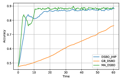
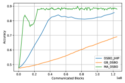
Figure 1: $\ell^{2}$-regularized logistic regression on synthetic data.

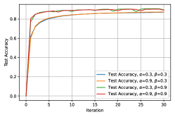
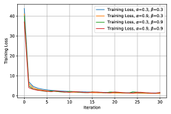
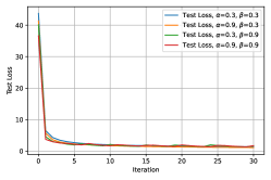
Figure 2: $\ell^{2}$-regularized logistic regression on MNIST.

4 Numerical experiments

In this section we study the applications of Algorithm 3 on hyperparameter optimization:

$$\min_{\lambda\in\mathbb{R}^{p}}\quad\frac{1}{n}\sum_{i=1}^{n}f_{i}(\lambda,\omega^{*}(\lambda)),$$

$$\text{s.t.}\quad\omega^{*}(\lambda)=\operatorname*{arg\,min}_{w\in\mathbb{R}^{q}}\frac{1}{n}\sum_{i=1}^{n}g_{i}(\lambda,\omega),$$

where we aim at finding the optimal hyperparameter $\lambda$ under the constraint that $\omega^{*}(\lambda)$ is the optimal model parameter given $\lambda$. We consider both the synthetic and real world data. Comparing to hypergradient estimation algorithms in Chen et al. (2022b) and Yang et al. (2022), our HIGP oracle (Algorithm 1) reduces both the per-iteration complexity and storage from $\mathcal{O}(q^{2})$ to $\mathcal{O}(q)$. All the experiments are performed on a local device with $8$ cores ($n=8$) using mpi4py (Dalcin & Fang, 2021) for parallel computing and PyTorch (Paszke et al., 2019) for computing stochastic oracles. The network topology is set to be the ring topology with the weight matrix $W=(w_{ij})$ given by

$$w_{ii}=w,\ w_{i,i+1}=w_{i,i-1}=\frac{1-w}{2},\ \text{for some }w\in(0,1).$$

Here $w_{1,0}=w_{1,n}$ and $w_{n,n+1}=w_{n,1}$. In other words, the neighbors of agent $i$ only include $i-1$ and $i+1$ for $i=1,2,...,n$ with $0$ and $n+1$ representing $n$ and $1$ respectively.

4.1 Heterogeneous and normally distributed data

Following Pedregosa (2016); Grazzi et al. (2020); Chen et al. (2022b), $f_{i}$ and $g_{i}$ are defined as:

$$f_{i}(\lambda,\omega)=\sum_{(x_{e},y_{e})\in\mathcal{D}_{i}^{\prime}}\psi(y_{e}x_{e}^{\top}\omega),$$

$$g_{i}(\lambda,\omega)=\sum_{(x_{e},y_{e})\in\mathcal{D}_{i}}\psi(y_{e}x_{e}^{\top}\omega)+\frac{1}{2}\sum_{i=1}^{p}e^{\lambda_{i}}\omega_{i}^{2},$$

where $\psi(x)=\log(1+e^{-x})$ and $p=200$ denotes the dimension parameter. A ground truth vector $w^{*}$ is generated in the beginning, and each $x_{e}\in\mathbb{R}^{p}$ is generated according to the normal distribution. The data distribution of $x_{e}$ on node $i$ is $\mathcal{N}(0,i^{2})$. Then we set $y_{e}=x_{e}^{\top}w+\varepsilon\cdot z$, where $\varepsilon=0.1$ denotes the noise rate and $z\in\mathbb{R}^{p}$ is the noise vector sampled from standard normal distribution. The task is to learn the optimal regularization parameter $\lambda\in\mathbb{R}^{p}$. We also compare our Algorithm 3 with GBDSBO (Yang et al., 2022) and DSBO-JHIP (Chen et al., 2022b) under this setting with dimension parameter $p=100$. Figures 1, 1 and 1 demonstrate the efficiency of our algorithm in both time and space complexity. Due to space limit, we include our additional experiments in Section A.

4.2 MNIST

Now we consider hyperparameter optimization on MNIST dataset (LeCun et al., 1998). Following Grazzi et al. (2020), we have

$$f_{i}(\lambda,\omega)=\frac{1}{|\mathcal{D}_{i}^{\prime}|}\sum_{(x_{e},y_{e})\in\mathcal{D}_{i}^{\prime}}L(x_{e}^{\top}\omega,y_{e}),$$

$$g_{i}(\lambda,\omega)=\frac{1}{|D_{i}|}\sum_{(x_{e},y_{e})\in\mathcal{D}_{i}}L(x_{e}^{\top}\omega,y_{e})+\frac{1}{cp}\sum_{i=1}^{c}\sum_{j=1}^{p}e^{\lambda_{j}}\omega_{ij}^{2},$$

where $c=10,\ p=784$ denote the number of classes and the number of features, $\omega\in\mathbb{R}^{c\times p}$ is the model parameter, and $L$ denotes the cross entropy loss. $\mathcal{D}_{i}$ and $\mathcal{D}_{i}^{\prime}$ denote the training and validation set respectively. The batch size is $1000$ in each stochastic oracle. We include the numerical results of different stepsize choices in Figure 2. Note that in previous algorithms (Chen et al., 2022b; Yang et al., 2022) one Hessian matrix of the lower level function requires $\mathcal{O}(c^{2}p^{2})$ storage, while in our algorithm a Hessian-vector product only requires $\mathcal{O}(cp)$ storage, which improves both the space and the communication complexity. The accuracy and the loss curves indicate that our MA-DSBO Algorithm 3 has a considerably good performance on real world dataset. Note that this problem has larger dimension, and the other algorithms took more time so we do not do the comparison.

5 Conclusion

In this paper, we propose a DSBO algorithm that does not require computing full Hessian and Jacobian matrices, thereby improving the per-iteration complexity of currently known DSBO algorithms, under mild assumptions. Moreover, we prove that our algorithm achieves $\tilde{\mathcal{O}}(\epsilon^{-2})$ sample complexity, which matches the result in state-of-the-art single-agent bilevel optimization algorithms. We would like to point out that Assumption 2.3 (or bounded second moment condition in Yang et al. (2022)) requires certain types of upper bounds on $\|\nabla_{y}g(x,y)\|$, which may not hold in decentralized optimization (see, e.g., Pu & Nedić (2021)). It is interesting to study decentralized stochastic bilevel optimization without this type of conditions, and one promising direction is to apply variance reduction techniques like in Tang et al. (2018). It is also interesting to incorporate Hessian-free methods (Sow et al., 2022) in DSBO, and we leave it as future work.

Acknowledgments

XC acknowledges the support by UC Davis Dean’s Graduate Summer Fellowship. Research of SM was supported in part by National Science Foundation (NSF) grants DMS-2243650, CCF-2308597, UC Davis CeDAR (Center for Data Science and Artificial Intelligence Research) Innovative Data Science Seed Funding Program, and a startup fund from Rice University. KB acknowledges the support by National Science Foundation (NSF) via the grant NSF DMS-2053918.

Appendix A Additional experiments on heterogeneous data

To introduce heterogeneity, we set $r$ as the heterogeneity rate, and the data distribution of $x_{e}$ in Section 4.1 on node $i$ is $\mathcal{N}(0,i^{2}\cdot r^{2})$. In Figure 3, 3 and 3 (and similarly for 3, 3, and 3) we set $r$ as $0.5,1.0,$ and $1.5$ respectively. The accuracy and loss results demonstrate that our algorithm works well under different heterogeneity rates.

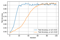
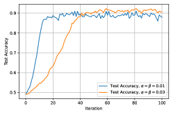
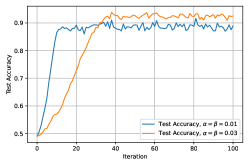
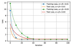
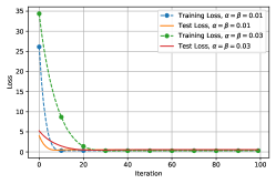
Figure 3: $\ell^{2}$-regularized logistic regression on synthetic data.

Appendix B Analysis

Figure 4 represents the structure of the proof. For convenience we restate our notation convention here again:

• We use the first subscript (usually denoted as $i$) to represent the agent number, and the second subscript (usually denoted as $k$ or $t$) to represent the iteration number. For example $x_{i,k}$ represents the $x$ variable of agent $i$ at $k$-th iteration. For the inner loop iterate like $y_{i,k}^{(t)}$, the superscript $t$ represents the iteration number of the inner loop.

• We use uppercase letters to represent the matrix that collecting all the variables (corresponding lowercase) as columns. For example $X_{k}=\left(x_{1,k},...,x_{n,k}\right),\ Y_{k}^{(t)}=\left(y_{1,k}^{(t)},...,y_{n,k}^{(t)}\right)$.

• We add an overbar to a letter to denote the average over all nodes. For example, $\bar{x}_{k}=\frac{1}{n}\sum_{i=1}^{n}x_{i,k},\ \bar{y}_{k}^{(t)}=\frac{1}{n}\sum_{i=1}^{n}y_{i,k}^{(t)}$.

• The filtration is defined as

  $$\mathcal{F}_{k}=\sigma\left(\bigcup_{i=1}^{n}\{y_{i,0}^{(T)},...,y_{i,k}^{(T)},x_{i,0},...,x_{i,k},r_{i,0},...,r_{i,k}\}\right).$$

Figure 4: Structure of the proof

We first state several well-known results in bilevel optimization literature (see, e.g., Lemma 2.2 in Ghadimi & Wang (2018).).

Lemma B.1.

Suppose Assumptions 2.1 and 2.4 hold, we know $\nabla\Phi(x)$ and $y^{*}(x)$ defined in (2) are $L_{\Phi}$ and $L_{y^{*}}$-Lipschitz continuous respectively with the constants given by

$$L_{\Phi}=L_{f,1}+\frac{2L_{f,1}L_{g,1}+L_{g,2}L_{f,0}^{2}}{\mu_{g}}+\frac{2L_{g,1}L_{f,0}L_{g,2}+L_{g,1}^{2}L_{f,1}}{\mu_{g}^{2}}+\frac{L_{g,2}L_{g,1}^{2}L_{f,0}}{\mu_{g}^{3}},\ L_{y^{*}}=\frac{L_{g,1}}{\mu_{g}}.$$ (12)

The following inequality is a standard result and will be used in our later analysis. We prove it here for completeness.

Lemma B.2.

Suppose we are given two sequences $\{a_{k}\}$ and $\{b_{k}\}$ that satisfy

$$a_{k+1}\leq\delta a_{k}+b_{k},\ a_{k}\geq 0,\ b_{k}\geq 0\text{ for all }k\geq 0$$

for some $\delta\in(0,1)$. Then we have

$$a_{k+1}\leq\delta^{k+1}a_{0}+\sum_{i=0}^{k}b_{i}\delta^{k-i}.$$

Proof of Lemma B.2.

Setting $c_{i}=\frac{a_{i}}{\delta^{i}}$, we know

$$c_{i+1}\leq c_{i}+b_{i}\cdot\delta^{-i-1}\text{ for all }i\geq 0.$$

Taking summation on both sides ($i$ from $0$ to $k$) and multiplying $\delta^{k+1}$, we know for $k\geq 0$,

$$a_{k+1}\leq\delta^{k+1}a_{0}+\sum_{i=0}^{k}b_{i}\delta^{k-i},$$

which completes the proof. ∎

The following lemma is standard in stochastic optimization (see, e.g., Lemma 10 in Qu & Li (2017)).

Lemma B.3.

Suppose $f(x)$ is $\mu$-strongly convex and $L-smooth$. For any $x$ and $\eta<\frac{2}{\mu+L}$, define $x^{+}=x-\eta\nabla f(x),\ x^{*}=\operatorname*{arg\,min}f(x)$. Then we have

$$\|x^{+}-x^{*}\|\leq(1-\eta\mu)\|x-x^{*}\|$$

Next, we characterize the bounded second moment of the HIGP oracle. Note that Algorithm 1 is essentially decentralized stochastic gradient descent with gradient tracking on a strongly convex quadratic function.

Lemma B.4.

Suppose we are given matrices $A_{i}$ and vectors $b_{i}$ such that there exist $0<\mu<L$ such that $\mu I\preceq A_{i}\preceq LI$ for $1\leq i\leq n$. $W=(w_{ij})$ satisfies Assumption 2.2. The sequences $\{x_{i,k}\},\ \{s_{i,k}\}$ and $\{v_{i,k}\}$ satisfy for any $k\geq 0$ and $1\leq i\leq n$,

$$x_{i,k+1}=\sum_{j=1}^{n}w_{ij}x_{j,k}-\alpha s_{i,k},\ s_{i,k+1}=\sum_{j=1}^{n}w_{ij}s_{j,k}+v_{i,k+1}-v_{i,k},\ v_{i,k}=A_{i,k}x_{i,k}-b_{i,k},\ s_{i,0}=v_{i,0},$$

$$\mathbb{E}\left[A_{i,k}\right]=A_{i},\ \mathbb{E}\left[b_{i,k}\right]=b_{i},\ \mathbb{E}\left[\|A_{i,k}-A_{i}\|^{2}\right]\leq\sigma_{1}^{2},\ \mathbb{E}\left[\|b_{i,k}-b_{i}\|^{2}\right]\leq\sigma_{2}^{2}.$$

Moreover, we assume $A_{i,k},x_{j,k},b_{i,k}$ are independent for any $i,j\in\left\{1,...,n\right\}$, $\left\{A_{i,k}\right\}_{i=1}^{n}$ are independent and $\left\{b_{i,k}\right\}_{i=1}^{n}$ are independent. Define

$$\tilde{\sigma}_{1}^{2}=\sigma_{1}^{2}+L^{2},\ \tilde{\sigma}_{2}^{2}=\sigma_{2}^{2}+\max_{i}\|b_{i}\|^{2},\ x^{*}:=\left(\frac{1}{n}\sum_{i=1}^{n}A_{i}\right)^{-1}\left(\frac{1}{n}\sum_{i=1}^{n}b_{i}\right),$$

$$C_{1}=9\sigma_{1}^{2}+6\alpha^{2}\tilde{\sigma}_{1}^{2}+\frac{18\alpha^{2}\sigma_{1}^{2}\tilde{\sigma}_{1}^{2}}{n},\ C_{2}=12\tilde{\sigma}_{1}^{2}+9\sigma_{1}^{2}+12\alpha^{2}L^{2}\tilde{\sigma}_{1}^{2}+\frac{18\alpha^{2}\sigma_{1}^{2}\tilde{\sigma}_{1}^{2}}{n},$$

$$C_{3}=6\rho^{2}\tilde{\sigma}_{1}^{2},\ C_{4}=2\sigma_{2}^{2}+\frac{6\alpha^{2}\sigma_{2}^{2}\tilde{\sigma}_{1}^{2}}{n}+\left(9\sigma_{1}^{2}+\frac{18\alpha^{2}\sigma_{1}^{2}\tilde{\sigma}_{1}^{2}}{n}\right)\|x^{*}\|^{2},$$

$$c=\left(\frac{\alpha^{2}}{n}(3\sigma_{1}^{2}\|x^{*}\|^{2}+\sigma_{2}^{2}),\ 0,\ \frac{(1+\rho^{2})}{1-\rho^{2}}C_{4}\right)^{\top},\ M=\begin{pmatrix}M_{11}&M_{12}&0\\ 0&M_{22}&M_{23}\\ M_{31}&M_{32}&M_{33}\end{pmatrix},$$

$$M_{11}=1-\alpha\mu,\ M_{12}=\left(\frac{2\alpha}{\mu}+2\alpha^{2}\right)\tilde{\sigma}_{1}^{2},\ M_{22}=\frac{1+\rho^{2}}{2},\ M_{23}=\alpha^{2}\frac{1+\rho^{2}}{1-\rho^{2}}$$

$$M_{31}=\frac{1+\rho^{2}}{1-\rho^{2}}C_{1},\ M_{32}=\frac{1+\rho^{2}}{1-\rho^{2}}C_{2},\ M_{33}=\frac{1+\rho^{2}}{2}+\frac{1+\rho^{2}}{1-\rho^{2}}C_{3}\alpha^{2}.$$

If $\alpha$ satisfies

$$\left(1+\frac{\alpha\mu}{2}\right)(1-\alpha\mu)^{2}+\frac{3\alpha^{2}\sigma_{1}^{2}}{n}<1-\alpha\mu,\ 0<\alpha_{1}\leq\alpha\leq\alpha_{2}\text{ for some }0<\alpha_{1}<\alpha_{2},$$ (13)

$$\rho(M)<1-\frac{2\alpha\mu}{3},\ \text{ and }~{}M~{}\text{has 3 different positive eigenvalues,}$$

then we have

$$\begin{aligned} \mathbb{E}\left[\|\bar{x}_{k+1}-x^{*}\|^{2}\right]&\leq(1-\alpha\mu)\mathbb{E}\left[\|\bar{x}_{k}-x^{*}\|^{2}\right]+\left(\frac{2\alpha}{\mu}+2\alpha^{2}\right)\frac{\tilde{\sigma}_{1}^{2}}{n}\mathbb{E}\left[\|X_{k}-\bar{x}_{k}\mathbf{1}^{\top}\|^{2}\right]\\ &\qquad+\frac{\alpha^{2}}{n}(3\sigma_{1}^{2}\|x^{*}\|^{2}+\sigma_{2}^{2}),\\ \|X_{k+1}-\bar{x}_{k+1}\mathbf{1}^{\top}\|^{2}&\leq\frac{(1+\rho^{2})}{2}\|X_{k}-\bar{x}_{k}\mathbf{1}^{\top}\|^{2}+\alpha^{2}\frac{1+\rho^{2}}{1-\rho^{2}}\|S_{k}-\bar{s}_{k}\mathbf{1}^{\top}\|^{2},\\ \mathbb{E}\left[\frac{\|S_{k+1}-\bar{s}_{k+1}\mathbf{1}^{\top}\|^{2}}{n}\right]&\leq\frac{1+\rho^{2}}{1-\rho^{2}}C_{1}\mathbb{E}\left[\|\bar{x}_{k}-x^{*}\|^{2}\right]+\frac{1+\rho^{2}}{1-\rho^{2}}C_{2}\mathbb{E}\left[\frac{\|X_{k}-\bar{x}_{k}\mathbf{1}^{\top}\|^{2}}{n}\right]\\ &\qquad\qquad+\left(\frac{1+\rho^{2}}{2}+\frac{1+\rho^{2}}{1-\rho^{2}}C_{3}\alpha^{2}\right)\mathbb{E}\left[\frac{\|S_{k}-\bar{s}_{k}\mathbf{1}^{\top}\|^{2}}{n}\right]+\frac{1+\rho^{2}}{1-\rho^{2}}C_{4}.\end{aligned}$$ (14)

Moreover, we set $P$ such that $M=P\cdot\text{diag}(\lambda_{1},\lambda_{2},\lambda_{3})P^{-1}$ with $0<\lambda_{3}<\lambda_{2}<\lambda_{1}$ being eigenvalues and each column of $P$ is a unit vector. Define $C_{M}:=\|P\|_{2}\|P^{-1}\|_{2}$, we have

$$\max\left(\frac{1}{n}\mathbb{E}\left[\|X_{k}-x^{*}\mathbf{1}^{\top}\|^{2}\right],\frac{1}{n}\mathbb{E}\left[\|X_{k}-\bar{x}_{k}\mathbf{1}^{\top}\|^{2}\right]\right)$$

$$\leq 3C_{M}\left(1-\frac{2\alpha\mu}{3}\right)^{k}\left(\mathbb{E}\left[\|\bar{x}_{0}-x^{*}\|^{2}\right]+\mathbb{E}\left[\frac{\|X_{0}\|^{2}+\|S_{0}\|^{2}}{n}\right]\right)+\frac{5C_{M}\|c\|}{\alpha\mu},$$ (15)

$$\frac{1}{n}\mathbb{E}\left[\|X_{k}\|^{2}\right]\leq 6C_{M}\left(1-\frac{2\alpha\mu}{3}\right)^{k}\left(\mathbb{E}\left[\|\bar{x}_{0}-x^{*}\|^{2}\right]+\mathbb{E}\left[\frac{\|X_{0}\|^{2}+\|S_{0}\|^{2}}{n}\right]\right)+\frac{10C_{M}\|c\|}{\alpha\mu}+2\|x^{*}\|^{2}.$$ (16)

Proof of Lemma B.4.

Note that by definition of $\tilde{\sigma}_{1}^{2}$ and $\tilde{\sigma}_{2}^{2}$ we have

$$\mathbb{E}\left[\|A_{i,k}\|^{2}\right]=\mathbb{E}\left[\|A_{i,k}-A_{i}\|^{2}\right]+\|A_{i}\|_{2}^{2}\leq\sigma_{1}^{2}+L^{2}=\tilde{\sigma}_{1}^{2},$$ (17)

$$\mathbb{E}\left[\|b_{i,k}\|^{2}\right]=\mathbb{E}\left[\|b_{i,k}-b_{i}\|^{2}\right]+\|b_{i}\|^{2}\leq\sigma_{2}^{2}+\max_{i}\|b_{i}\|^{2}=\tilde{\sigma}_{2}^{2}.$$

By $s_{i,0}=v_{i,0}$ we know $\bar{s}_{0}=\bar{v}_{0}$. From the recursion we know

$$\bar{s}_{k+1}=\bar{s}_{k}+\bar{v}_{k+1}-\bar{v}_{k},$$

and hence $\bar{s}_{k}=\bar{v}_{k}$ by induction. For $\bar{x}_{k}$ we know

$$\bar{x}_{k+1}-x^{*}$$

$$= \bar{x}_{k}-x^{*}-\frac{\alpha}{n}\sum_{i=1}^{n}(A_{i,k}x_{i,k}-b_{i,k})$$

$$= \bar{x}_{k}-x^{*}-\frac{\alpha}{n}\sum_{i=1}^{n}(A_{i}\bar{x}_{k}-b_{i})+\frac{\alpha}{n}\sum_{i=1}^{n}(A_{i}\bar{x}_{k}-b_{i})-\frac{\alpha}{n}\sum_{i=1}^{n}(A_{i,k}x_{i,k}-b_{i,k})$$

$$= \left(I-\frac{\alpha}{n}\sum_{i=1}^{n}A_{i}\right)(\bar{x}_{k}-x^{*})+\frac{\alpha}{n}\sum_{i=1}^{n}A_{i,k}(\bar{x}_{k}-x_{i,k})+\frac{\alpha}{n}\sum_{i=1}^{n}((A_{i}-A_{i,k})\bar{x}_{k}+b_{i,k}-b_{i}).$$

Using the above equality, $\mathbb{E}\left[A_{i,k}\right]=A_{i}$ and $\mathbb{E}\left[b_{i,k}\right]=b_{i}$, we know

$$\mathbb{E}\left[\|\bar{x}_{k+1}-x^{*}\|^{2}\right]$$

$$= \mathbb{E}\left[\|\left(I-\frac{\alpha}{n}\sum_{i=1}^{n}A_{i}\right)(\bar{x}_{k}-x^{*})+\frac{\alpha}{n}\sum_{i=1}^{n}A_{i,k}(\bar{x}_{k}-x_{i,k})\|^{2}\right]+\frac{\alpha^{2}}{n^{2}}\mathbb{E}\left[\|\sum_{i=1}^{n}((A_{i}-A_{i,k})\bar{x}_{k}+b_{i,k}-b_{i})\|^{2}\right]$$

$$+ \mathbb{E}\left[\langle\left(I-\frac{\alpha}{n}\sum_{i=1}^{n}A_{i}\right)(\bar{x}_{k}-x^{*})+\frac{\alpha}{n}\sum_{i=1}^{n}A_{i,k}(\bar{x}_{k}-x_{i,k}),\frac{\alpha}{n}\sum_{i=1}^{n}((A_{i}-A_{i,k})\bar{x}_{k}+b_{i,k}-b_{i})\rangle\right]$$

$$\leq \left(1+\frac{\alpha\mu}{2}\right)(1-\alpha\mu)^{2}\mathbb{E}\left[\|\bar{x}_{k}-x^{*}\|^{2}\right]+\left(1+\frac{2}{\alpha\mu}\right)\frac{\alpha^{2}\tilde{\sigma}_{1}^{2}}{n}\sum_{i=1}^{n}\mathbb{E}\left[\|\bar{x}_{k}-x_{i,k}\|^{2}\right]+\frac{\alpha^{2}}{n^{2}}(n\sigma_{1}^{2}\mathbb{E}\left[\|\bar{x}_{k}\|^{2}\right]+n\sigma_{2}^{2})$$

$$+ \frac{\alpha^{2}}{2n^{2}}\sum_{i=1}^{n}\mathbb{E}\left[\sigma_{1}^{2}\|\bar{x}_{k}\|^{2}+\tilde{\sigma}_{1}^{2}\|\bar{x}_{k}-x_{i,k}\|^{2}\right]$$

$$= \left(1+\frac{\alpha\mu}{2}\right)(1-\alpha\mu)^{2}\mathbb{E}\left[\|\bar{x}_{k}-x^{*}\|^{2}\right]+\left(\frac{2\alpha}{\mu}+\alpha^{2}+\frac{\alpha^{2}}{2n}\right)\frac{\tilde{\sigma}_{1}^{2}}{n}\mathbb{E}\left[\|X_{k}-\bar{x}_{k}\mathbf{1}^{\top}\|^{2}\right]+\frac{\alpha^{2}}{n}\left(\frac{3\sigma_{1}^{2}}{2}\mathbb{E}\left[\|\bar{x}_{k}\|^{2}\right]+\sigma_{2}^{2}\right)$$

$$\leq \left[\left(1+\frac{\alpha\mu}{2}\right)(1-\alpha\mu)^{2}+\frac{3\alpha^{2}\sigma_{1}^{2}}{n}\right]\mathbb{E}\left[\|\bar{x}_{k}-x^{*}\|^{2}\right]+\left(\frac{2\alpha}{\mu}+2\alpha^{2}\right)\frac{\tilde{\sigma}_{1}^{2}}{n}\mathbb{E}\left[\|X_{k}-\bar{x}_{k}\mathbf{1}^{\top}\|^{2}\right]+\frac{\alpha^{2}}{n}(3\sigma_{1}^{2}\|x^{*}\|^{2}+\sigma_{2}^{2})$$

$$\leq (1-\alpha\mu)\mathbb{E}\left[\|\bar{x}_{k}-x^{*}\|^{2}\right]+\left(\frac{2\alpha}{\mu}+2\alpha^{2}\right)\frac{\tilde{\sigma}_{1}^{2}}{n}\mathbb{E}\left[\|X_{k}-\bar{x}_{k}\mathbf{1}^{\top}\|^{2}\right]+\frac{\alpha^{2}}{n}(3\sigma_{1}^{2}\|x^{*}\|^{2}+\sigma_{2}^{2}).$$

The first inequality holds because we have

$$\mathbb{E}\left[\langle\left(I-\frac{\alpha}{n}\sum_{i=1}^{n}A_{i}\right)(\bar{x}_{k}-x^{*})+\frac{\alpha}{n}\sum_{i=1}^{n}A_{i,k}(\bar{x}_{k}-x_{i,k}),\frac{\alpha}{n}\sum_{i=1}^{n}((A_{i}-A_{i,k})\bar{x}_{k}+b_{i,k}-b_{i})\rangle\right]$$

$$= \mathbb{E}\left[\langle\frac{\alpha}{n}\sum_{i=1}^{n}A_{i,k}(\bar{x}_{k}-x_{i,k}),\frac{\alpha}{n}\sum_{i=1}^{n}((A_{i}-A_{i,k})\bar{x}_{k}+b_{i,k}-b_{i})\rangle\right]$$

$$= \mathbb{E}\left[\langle\frac{\alpha}{n}\sum_{i=1}^{n}A_{i,k}(\bar{x}_{k}-x_{i,k}),\frac{\alpha}{n}\sum_{i=1}^{n}(A_{i}-A_{i,k})\bar{x}_{k}\rangle\right]$$

$$= \frac{\alpha^{2}}{n^{2}}\sum_{i=1}^{n}\mathbb{E}\left[(\bar{x}_{k}-x_{i,k})^{\top}A_{i,k}^{\top}(A_{i}-A_{i,k})\bar{x}_{k}\right]\leq\frac{\alpha^{2}}{2n^{2}}\sum_{i=1}^{n}\mathbb{E}\left[\sigma_{1}^{2}\|\bar{x}_{k}\|^{2}+\tilde{\sigma}_{1}^{2}\|\bar{x}_{k}-x_{i,k}\|^{2}\right],$$

the second inequality uses $\|\bar{x}_{k}\|^{2}\leq 2\|\bar{x}_{k}-x^{*}\|^{2}+2\|x^{*}\|^{2}$, and the third inequality uses (13). For $\|X_{k+1}-\bar{x}_{k+1}\mathbf{1}^{\top}\|^{2}$ we know

$$\|X_{k+1}-\bar{x}_{k+1}\mathbf{1}^{\top}\|^{2}=\|X_{k}W-\bar{x}_{k}\mathbf{1}^{\top}-\alpha(S_{k}-\bar{s}_{k}\mathbf{1}^{\top})\|^{2}$$ (18)

$$\leq \left(1+\frac{1-\rho^{2}}{2\rho^{2}}\right)\rho^{2}\|X_{k}-\bar{x}_{k}\mathbf{1}^{\top}\|^{2}+\left(1+\frac{2\rho^{2}}{1-\rho^{2}}\right)\alpha^{2}\|S_{k}-\bar{s}_{k}\mathbf{1}^{\top}\|^{2}.$$

The inequality uses Cauchy-Schwarz inequality and the fact that

$$\|X_{k}W-\bar{x}_{k}\mathbf{1}^{\top}\|=\|\left(X_{k}-\bar{x}_{k}\mathbf{1}^{\top}\right)\left(W-\frac{\mathbf{1}\mathbf{1}^{\top}}{n}\right)\|=\|\left(W-\frac{\mathbf{1}\mathbf{1}^{\top}}{n}\right)\left(X_{k}-\bar{x}_{k}\mathbf{1}^{\top}\right)^{\top}\|$$

$$\leq \|W-\frac{\mathbf{1}\mathbf{1}^{\top}}{n}\|_{2}\|X_{k}-\bar{x}_{k}\mathbf{1}^{\top}\|\leq\rho\|X_{k}-\bar{x}_{k}\mathbf{1}^{\top}\|,$$

where the last inequality uses Assumption 2.2. For $\|S_{k}-\bar{s}_{k}\mathbf{1}^{\top}\|^{2}$ we know

$$\|S_{k+1}-\bar{s}_{k+1}\mathbf{1}^{\top}\|^{2}=\|S_{k}W-\bar{s}_{k}\mathbf{1}^{\top}+V_{k+1}-V_{k}-\bar{v}_{k+1}\mathbf{1}^{\top}+\bar{v}_{k}\mathbf{1}^{\top}\|^{2}$$ (19)

$$\leq \left(1+\frac{1-\rho^{2}}{2\rho^{2}}\right)\|S_{k}-\bar{s}_{k}\mathbf{1}^{\top}\|^{2}+\left(1+\frac{2\rho^{2}}{1-\rho^{2}}\right)\|\left(V_{k+1}-V_{k}\right)\left(I-\frac{\mathbf{1}\mathbf{1}^{\top}}{n}\right)\|^{2}$$

$$= \frac{1+\rho^{2}}{2}\|S_{k}-\bar{s}_{k}\mathbf{1}^{\top}\|^{2}+\frac{1+\rho^{2}}{1-\rho^{2}}\|V_{k+1}-V_{k}\|^{2}.$$

For $V_{k+1}-V_{k}$ we have

$$\mathbb{E}\left[\|V_{k+1}-V_{k}\|^{2}\right]$$

$$= \sum_{i=1}^{n}\mathbb{E}\left[\|A_{i,k+1}(x_{i,k+1}-x_{i,k})+(A_{i,k+1}-A_{i}+A_{i}-A_{i,k})x_{i,k}+(b_{i,k}-b_{i}+b_{i}-b_{i,k+1})\|^{2}\right]$$

$$= \sum_{i=1}^{n}\mathbb{E}\left[\|A_{i,k+1}(x_{i,k+1}-x_{i,k})+(A_{i,k+1}-A_{i})x_{i,k}\|^{2}+\|(A_{i}-A_{i,k})x_{i,k}\|^{2}+\|b_{i,k}-b_{i}\|^{2}+\|b_{i}-b_{i,k+1}\|^{2}\right]$$

$$\leq \sum_{i=1}^{n}\mathbb{E}\left[2\|A_{i,k+1}(x_{i,k+1}-x_{i,k})\|^{2}+2\|(A_{i,k+1}-A_{i})x_{i,k}\|^{2}+\|(A_{i}-A_{i,k})x_{i,k}\|^{2}+\|b_{i,k}-b_{i}\|^{2}+\|b_{i}-b_{i,k+1}\|^{2}\right]$$

$$\leq 2\tilde{\sigma}_{1}^{2}\mathbb{E}\left[\|X_{k+1}-X_{k}\|^{2}\right]+3\sigma_{1}^{2}\mathbb{E}\left[\|X_{k}\|^{2}\right]+2n\sigma_{2}^{2}.$$

For $\|X_{k+1}-X_{k}\|$ we know

$$\mathbb{E}\left[\|X_{k+1}-X_{k}\|^{2}\right]=\mathbb{E}\left[\|X_{k}W-X_{k}-\alpha S_{k}W\|^{2}\right]$$

$$= \mathbb{E}\left[\|\left(X_{k}-\bar{x}_{k}\mathbf{1}^{\top}\right)(W-I)-\alpha(S_{k}W-\bar{s}_{k}\mathbf{1}^{\top})-\alpha\bar{s}_{k}\mathbf{1}^{\top}\|^{2}\right]$$

$$\leq 3\|W-I\|_{2}^{2}\mathbb{E}\left[\|X_{k}-\bar{x}_{k}\mathbf{1}^{\top}\|^{2}\right]+3\alpha^{2}\rho^{2}\mathbb{E}\left[\|S_{k}-\bar{s}_{k}\mathbf{1}^{\top}\|^{2}\right]+3n\alpha^{2}\mathbb{E}\left[\|\bar{s}_{k}\|^{2}\right]$$

$$\leq 6\mathbb{E}\left[\|X_{k}-\bar{x}_{k}\mathbf{1}^{\top}\|^{2}\right]+3\alpha^{2}\rho^{2}\mathbb{E}\left[\|S_{k}-\bar{s}_{k}\mathbf{1}^{\top}\|^{2}\right]$$

$$\qquad\qquad+3\alpha^{2}(\frac{\sigma_{1}^{2}}{n}\mathbb{E}\left[\|X_{k}\|^{2}\right]+\sigma_{2}^{2}+2L^{2}\mathbb{E}\left[\|X_{k}-\bar{x}_{k}\mathbf{1}^{\top}\|^{2}+n\|\bar{x}_{k}-x^{*}\|^{2}\right])$$

$$= (6+6\alpha^{2}L^{2})\mathbb{E}\left[\|X_{k}-\bar{x}_{k}\mathbf{1}^{\top}\|^{2}\right]+3\alpha^{2}\rho^{2}\mathbb{E}\left[\|S_{k}-\bar{s}_{k}\mathbf{1}^{\top}\|^{2}\right]+\frac{3\alpha^{2}\sigma_{1}^{2}}{n}\mathbb{E}\left[\|X_{k}\|^{2}\right]$$

$$\qquad\qquad+3n\alpha^{2}\mathbb{E}\left[\|\bar{x}_{k}-x^{*}\|^{2}\right]+3\alpha^{2}\sigma_{2}^{2},$$

where the second inequality holds since

$$\mathbb{E}\left[\|\bar{s}_{k}\|^{2}\right]=\mathbb{E}\left[\|\frac{1}{n}\sum_{i=1}^{n}(A_{i,k}x_{i,k}-b_{i,k})\|^{2}\right]$$

$$= \mathbb{E}\left[\|\frac{1}{n}\sum_{i=1}^{n}((A_{i,k}-A_{i})x_{i,k}-(b_{i,k}-b_{i}))+\frac{1}{n}\sum_{i=1}^{n}(A_{i}x_{i,k}-A_{i}\bar{x}_{k})+\frac{1}{n}\sum_{i=1}^{n}A_{i}(\bar{x}_{k}-x^{*})\|^{2}\right]$$

$$= \frac{1}{n^{2}}\sum_{i=1}^{n}\mathbb{E}\left[\|(A_{i,k}-A_{i})x_{i,k}\|^{2}+\|b_{i,k}-b_{i}\|^{2}\right]+\frac{1}{n^{2}}\mathbb{E}\left[\|\sum_{i=1}^{n}((A_{i}x_{i,k}-A_{i}\bar{x}_{k})+A_{i}(\bar{x}_{k}-x^{*}))\|^{2}\right]$$

$$\leq \frac{\sigma_{1}^{2}}{n^{2}}\mathbb{E}\left[\|X_{k}\|^{2}\right]+\frac{\sigma_{2}^{2}}{n}+\frac{2L^{2}}{n}\mathbb{E}\left[\|X_{k}-\bar{x}_{k}\mathbf{1}^{\top}\|^{2}+n\|\bar{x}_{k}-x^{*}\|^{2}\right].$$

Hence we know

$$\mathbb{E}\left[\|V_{k+1}-V_{k}\|^{2}\right]\leq 2\tilde{\sigma}_{1}^{2}\mathbb{E}\left[\|X_{k+1}-X_{k}\|^{2}\right]+3\sigma_{1}^{2}\mathbb{E}\left[\|X_{k}\|^{2}\right]+2n\sigma_{2}^{2}$$

$$\leq 2\tilde{\sigma}_{1}^{2}\left\{(6+6\alpha^{2}L^{2})\mathbb{E}\left[\|X_{k}-\bar{x}_{k}\mathbf{1}^{\top}\|^{2}\right]+3\alpha^{2}\rho^{2}\mathbb{E}\left[\|S_{k}-\bar{s}_{k}\mathbf{1}^{\top}\|^{2}\right]+3n\alpha^{2}\mathbb{E}\left[\|\bar{x}_{k}-x^{*}\|^{2}\right]\right\}$$

$$+ \left(3\sigma_{1}^{2}+\frac{6\alpha^{2}\sigma_{1}^{2}\tilde{\sigma}_{1}^{2}}{n}\right)\mathbb{E}\left[\|X_{k}\|^{2}\right]+(2n\sigma_{2}^{2}+6\alpha^{2}\sigma_{2}^{2}\tilde{\sigma}_{1}^{2})$$

$$\leq nC_{1}\mathbb{E}\left[\|\bar{x}_{k}-x^{*}\|^{2}\right]+C_{2}\mathbb{E}\left[\|X_{k}-\bar{x}_{k}\mathbf{1}^{\top}\|^{2}\right]+\alpha^{2}C_{3}\mathbb{E}\left[\|S_{k}-\bar{s}_{k}\mathbf{1}^{\top}\|^{2}\right]+nC_{4},$$

where the second inequality uses

$$\|X_{k}\|^{2}\leq 3\left[\|X_{k}-\bar{x}_{k}\mathbf{1}^{\top}\|^{2}+n\|\bar{x}_{k}-x^{*}\|^{2}+n\|x^{*}\|^{2}\right].$$

The above inequalities and (19) imply

$$\frac{1}{n}\mathbb{E}\left[\|S_{k+1}-\bar{s}_{k+1}\mathbf{1}^{\top}\|^{2}\right]$$ (20)

$$\leq \frac{1+\rho^{2}}{2n}\|S_{k}-\bar{s}_{k}\mathbf{1}^{\top}\|^{2}+\frac{1+\rho^{2}}{1-\rho^{2}}\left(C_{1}\mathbb{E}\left[\|\bar{x}_{k}-x^{*}\|^{2}\right]+C_{2}\mathbb{E}\left[\frac{\|X_{k}-\bar{x}_{k}\mathbf{1}^{\top}\|^{2}}{n}\right]+\alpha^{2}C_{3}\mathbb{E}\left[\frac{\|S_{k}-\bar{s}_{k}\mathbf{1}^{\top}\|^{2}}{n}\right]+C_{4}\right)$$

$$\leq \frac{1+\rho^{2}}{1-\rho^{2}}C_{1}\mathbb{E}\left[\|\bar{x}_{k}-x^{*}\|^{2}\right]+\frac{1+\rho^{2}}{1-\rho^{2}}C_{2}\mathbb{E}\left[\frac{\|X_{k}-\bar{x}_{k}\mathbf{1}^{\top}\|^{2}}{n}\right]+\left(\frac{1+\rho^{2}}{2}+\frac{1+\rho^{2}}{1-\rho^{2}}C_{3}\alpha^{2}\right)\mathbb{E}\left[\frac{\|S_{k}-\bar{s}_{k}\mathbf{1}^{\top}\|^{2}}{n}\right]+\frac{1+\rho^{2}}{1-\rho^{2}}C_{4}.$$

Now if we define

$$\Gamma_{k}=\left(\mathbb{E}\left[\|\bar{x}_{k}-x^{*}\|^{2}\right],\ \mathbb{E}\left[\frac{\|X_{k}-\bar{x}_{k}\mathbf{1}^{\top}\|^{2}}{n}\right],\ \mathbb{E}\left[\frac{\|S_{k}-\bar{s}_{k}\mathbf{1}^{\top}\|^{2}}{n}\right]\right)^{\top},\$$

$$c=\left(\frac{\alpha^{2}}{n}(3\sigma_{1}^{2}\|x^{*}\|^{2}+\sigma_{2}^{2}),\ 0,\ \frac{(1+\rho^{2})}{1-\rho^{2}}C_{4}\right)^{\top},\ M=\begin{pmatrix}M_{11}&M_{12}&0\\ 0&M_{22}&M_{23}\\ M_{31}&M_{32}&M_{33}\end{pmatrix},$$

$$M_{11}=1-\alpha\mu,\ M_{12}=\left(\frac{2\alpha}{\mu}+2\alpha^{2}\right)\tilde{\sigma}_{1}^{2},\ M_{22}=\frac{1+\rho^{2}}{2},\ M_{23}=\alpha^{2}\frac{1+\rho^{2}}{1-\rho^{2}}$$

$$M_{31}=\frac{1+\rho^{2}}{1-\rho^{2}}C_{1},\ M_{32}=\frac{1+\rho^{2}}{1-\rho^{2}}C_{2},\ M_{33}=\frac{1+\rho^{2}}{2}+\frac{1+\rho^{2}}{1-\rho^{2}}C_{3}\alpha^{2},$$

then by (14) we know $\Gamma_{i+1}\leq M\Gamma_{i}+c$ for any $i$, and thus

$$\Gamma_{k+1}\leq M\Gamma_{k}+c\leq...\leq M^{k+1}\Gamma_{0}+\sum_{i=0}^{k}M^{i}c,$$

where all the inequalities are element-wise. By (13) we know there exists an invertible matrix $P\in\mathbb{R}^{3\times 3}$ such that $M=P\cdot\text{diag}(\lambda_{1},\lambda_{2},\lambda_{3})P^{-1}$, and $0<\lambda_{3}<\lambda_{2}<\lambda_{1}<1-\frac{2\alpha\mu}{3}$. Without loss of generality we may assume each column of $P$ (as an eigenvector) is a unit vector. Hence we know

$$\|M^{k}\|_{2}=\|P\cdot\text{diag}(\lambda_{1}^{k},\lambda_{2}^{k},\lambda_{3}^{k})P^{-1}\|_{2}\leq\left(1-\frac{2\alpha\mu}{3}\right)^{k}\|P\|_{2}\|P^{-1}\|_{2}=C_{M}\cdot\left(1-\frac{2\alpha\mu}{3}\right)^{k},$$ (21)

where we define $C_{M}:=\|P\|_{2}\|P^{-1}\|_{2}$ in the last equality. Note that since we choose $P$ such that each column is a unit vector and $M=P\cdot\text{diag}(\lambda_{1},\lambda_{2},\lambda_{3})P^{-1}$, $P$ is uniquely determined and $C_{M}$ is a continuous function of $\alpha$ and other constants $(\sigma_{1},\ \sigma_{2},\ \mu,\ L,\ \max_{i}\|b_{i}\|,\ \|x^{*}\|,\ n,\ \rho)$. On the other hand, observe that

$$\begin{aligned} \|\sum_{i=0}^{k}M^{i}\|_{2}&=\|\sum_{i=0}^{k}P\cdot\text{diag}(\lambda_{1}^{i},\lambda_{2}^{i},\lambda_{3}^{i})P^{-1}\|_{2}=\|P\cdot\text{diag}\left(\sum_{i=0}^{k}\lambda_{1}^{i},\sum_{i=0}^{k}\lambda_{2}^{i},\sum_{i=0}^{k}\lambda_{3}^{i}\right)P^{-1}\|_{2}\\ &\leq C_{M}\cdot\max_{i}\frac{1}{1-\lambda_{i}}<\frac{3C_{M}}{2\alpha\mu},\end{aligned}$$ (22)

where the last inequality uses the upper bound of the eigenvalues. For (15) we have

$$\max\left(\frac{1}{n}\mathbb{E}\left[\|X_{k}-x^{*}\mathbf{1}^{\top}\|^{2}\right],\frac{1}{n}\mathbb{E}\left[\|X_{k}-\bar{x}_{k}\mathbf{1}^{\top}\|^{2}\right]\right)\leq\frac{2}{n}\mathbb{E}\left[\|X_{k}-\bar{x}_{k}\mathbf{1}^{\top}\|^{2}+n\|\bar{x}_{k}-x^{*}\|^{2}\right]\leq 2\sqrt{2}\|\Gamma_{k}\|$$

$$\leq 2\sqrt{2}\|M^{k}\Gamma_{0}+\sum_{i=0}^{k-1}M^{i}c\|\leq 2\sqrt{2}(\|M^{k}\|_{2}\|\Gamma_{0}\|+\|\sum_{i=1}^{k-1}M^{i}\|_{2}\|c\|)$$

$$\leq 2\sqrt{2}C_{M}\left(1-\frac{2\alpha\mu}{3}\right)^{k}\|\Gamma_{0}\|+2\sqrt{2}\cdot\frac{3C_{M}}{2\alpha\mu}\|c\|$$

$$\leq 2\sqrt{2}C_{M}\left(1-\frac{2\alpha\mu}{3}\right)^{k}(\mathbb{E}\left[\|\bar{x}_{0}-x^{*}\|^{2}\right]+\mathbb{E}\left[\frac{\|X_{0}-\bar{x}_{0}\mathbf{1}^{\top}\|^{2}}{n}\right]+\mathbb{E}\left[\frac{\|S_{0}-\bar{s}_{0}\mathbf{1}^{\top}\|^{2}}{n}\right])+\frac{3\sqrt{2}C_{M}\|c\|}{\alpha\mu}$$

$$\leq 3C_{M}\left(1-\frac{2\alpha\mu}{3}\right)^{k}\left(\mathbb{E}\left[\|\bar{x}_{0}-x^{*}\|^{2}\right]+\mathbb{E}\left[\frac{\|X_{0}\|^{2}+\|S_{0}\|^{2}}{n}\right]\right)+\frac{5C_{M}\|c\|}{\alpha\mu},$$

where the fifth inequality uses (21) and (22), and the seventh inequality uses the fact that $\|X_{0}-\bar{x}_{0}\mathbf{1}^{\top}\|=\|X_{0}\left(I-\frac{\mathbf{1}\mathbf{1}^{\top}}{n}\right)\|\leq\|X_{0}\|$ (same for $S_{0}$). (16) can be viewed as a corollary of the above inequality by noticing that

$$\frac{1}{n}\mathbb{E}\left[\|X_{k}\|^{2}\right]\leq\frac{2}{n}\mathbb{E}\left[\|X_{k}-x^{*}\mathbf{1}^{\top}\|^{2}+n\|x^{*}\|^{2}\right]$$

$$\leq 6C_{M}\left(1-\frac{2\alpha\mu}{3}\right)^{k}\left(\mathbb{E}\left[\|\bar{x}_{0}-x^{*}\|^{2}\right]+\mathbb{E}\left[\frac{\|X_{0}\|^{2}+\|S_{0}\|^{2}}{n}\right]\right)+\frac{10C_{M}\|c\|}{\alpha\mu}+2\|x^{*}\|^{2}.$$

∎

Remark:

• Lemma B.4 characterizes convergence results of decentralized stochastic gradient descent with gradient tracking on strongly convex quadratic functions. Moreover, it also indicates that the second moment of $X_{k}$ can be bounded by using (16), which will be used in proving the boundedness of second moment of $Z_{t}^{(k)}$ of our HIGP oracle.

• If we consider the same updates under the deterministic setting, then $\sigma_{1}=\sigma_{2}=0$ and thus $\|c\|=0$ by definition, which indicates the constant term in (15) vanishes (i.e., linear convergence). We will utilize this important observation in the next lemma.

Lemma B.5.

Suppose Assumptions 2.1, 2.2 and 2.4 hold. In Algorithm 1 define

$$C_{1}=9\sigma_{g,2}^{2}+6\gamma^{2}(\sigma_{g,2}^{2}+L_{g,1}^{2})+\frac{18\gamma^{2}\sigma_{g,2}^{2}(\sigma_{g,2}^{2}+L_{g,1}^{2})}{n},$$

$$C_{2}=12(\sigma_{g,2}^{2}+L_{g,1}^{2})+9\sigma_{g,2}^{2}+12\gamma^{2}L_{g,1}^{2}(\sigma_{g,2}^{2}+L_{g,1}^{2})+\frac{18\gamma^{2}\sigma_{g,2}^{2}(\sigma_{g,2}^{2}+L_{g,1}^{2})}{n},$$

$$C_{3}=6\rho^{2}(\sigma_{g,2}^{2}+L_{g,1}^{2}),\ C_{4}=2\sigma_{f}^{2}+\frac{6\gamma^{2}\sigma_{f}^{2}(\sigma_{g,2}^{2}+L_{g,1}^{2})}{n}+(9\sigma_{g,2}^{2}+\frac{18\gamma^{2}\sigma_{g,2}^{2}(\sigma_{g,2}^{2}+L_{g,1}^{2})}{n})\|x^{*}\|^{2},$$

$$c=\left(\frac{\gamma^{2}}{n}\left(3\sigma_{g,2}^{2}\frac{L_{f,0}^{2}}{\mu_{g}^{2}}+\sigma_{f}^{2}\right),\ 0,\ \frac{(1+\rho^{2})}{1-\rho^{2}}C_{4}\right)^{\top},\ M=\begin{pmatrix}M_{11}&M_{12}&0\\ 0&M_{22}&M_{23}\\ M_{31}&M_{32}&M_{33}\end{pmatrix},$$

$$M_{11}=1-\gamma\mu_{g},\ M_{12}=\left(\frac{2\gamma}{\mu_{g}}+2\gamma^{2}\right)(\sigma_{g,2}^{2}+L_{g,1}^{2}),\ M_{22}=\frac{1+\rho^{2}}{2},\ M_{23}=\gamma^{2}\frac{1+\rho^{2}}{1-\rho^{2}},$$

$$M_{31}=\frac{1+\rho^{2}}{1-\rho^{2}}C_{1},\ M_{32}=\frac{1+\rho^{2}}{1-\rho^{2}}C_{2},\ M_{33}=\frac{1+\rho^{2}}{2}+\frac{1+\rho^{2}}{1-\rho^{2}}C_{3}\gamma^{2}.$$

Define $\tilde{M}$ to be matrix $M$ and $C_{\tilde{M}}$ to be $C_{M}$ when $\sigma_{g,2}=\sigma_{f}=0$. If $\gamma$ satisfies

$$\left(1+\frac{\gamma\mu_{g}}{2}\right)(1-\gamma\mu_{g})^{2}+\frac{3\gamma^{2}\sigma_{g,2}^{2}}{n}<1-\gamma\mu_{g},\ 0<\gamma_{1}\leq\gamma\leq\gamma_{2}\text{ for some }0<\gamma_{1}<\gamma_{2},$$ (23)

$$\max\left(\rho(\tilde{M}),\rho(M)\right)<1-\frac{2\gamma\mu_{g}}{3},\ \text{both }M\text{ and }\tilde{M}\text{have 3 different positive eigenvalues,}$$

then for any $0\leq t\leq N$ we have

$$\mathbb{E}\left[\|\bar{z}_{t}^{(k)}\|^{2}|\mathcal{F}_{k}\right]\leq\frac{1}{n}\mathbb{E}\left[\|Z_{t}^{(k)}\|^{2}|\mathcal{F}_{k}\right]\leq\sigma_{z}^{2}:=6C_{M}\left(\frac{L_{f,0}^{2}}{\mu_{g}^{2}}+\sigma_{f}^{2}+L_{f,0}^{2}\right)+\frac{10C_{M}\|c\|}{\gamma\mu_{g}}+\frac{2L_{f,0}^{2}}{\mu_{g}^{2}},$$ (24)

$$\frac{1}{n}\|\mathbb{E}\left[Z_{t}^{(k)}-\bar{z}_{t}^{(k)}\mathbf{1}^{\top}|\mathcal{F}_{k}\right]\|^{2}\leq 3C_{\tilde{M}}\left(1-\frac{2\gamma\mu_{g}}{3}\right)^{t}\left(\frac{L_{f,0}^{2}}{\mu_{g}^{2}}+L_{f,0}^{2}\right).$$ (25)

Proof of Lemma B.5.

Note that (24) is a direct results of Lemma B.4 by noticing that

$$z_{i,t+1}^{(k)}=\sum_{j=1}^{n}w_{ij}z_{j,t}^{(k)}-\gamma d_{i,t}^{(k)},\ Z_{0}^{(k)}=0,$$

$$d_{i,t+1}^{(k)}=\sum_{i=1}^{n}w_{ij}d_{j,t}^{(k)}+s_{i,t+1}^{(k)}-s_{i,t}^{(k)},\ s_{i,t}^{(k)}=H_{i,t}^{(k)}z_{i,t}^{(k)}-b_{i,t}^{(k)},$$

$$\mathbb{E}\left[H_{i,t}^{(k)}|\mathcal{F}_{k}\right]=\nabla_{y}^{2}g_{i}(x_{i,k},y_{i,k}^{(T)}),\ \mathbb{E}\left[\|H_{i,t}^{(k)}-\nabla_{y}^{2}g_{i}(x_{i,k},y_{i,k}^{(T)})\|^{2}|\mathcal{F}_{k}\right]\leq\sigma_{g,2}^{2},$$

$$\mathbb{E}\left[b_{i,t}^{(k)}|\mathcal{F}_{k}\right]=\nabla_{y}f_{i}(x_{i,k},y_{i,k}^{(T)}),\ \mathbb{E}\left[\|b_{i,t}^{(k)}-\nabla_{y}f_{i}(x_{i,k},y_{i,k}^{(T)})\|^{2}|\mathcal{F}_{k}\right]\leq\sigma_{f}^{2},$$

for any $k\geq 0,1\leq i\leq n,$ and $t\geq 0$. Assumption 2.1 also indicates that

$$\mu_{g}I\preceq\nabla_{y}^{2}g_{i}(x_{i,k},y_{i,k}^{(T)})\preceq L_{g,1}I,\ \|\nabla_{y}f_{i}(x_{i,k},y_{i,k}^{(T)})\|\leq L_{f,0}.$$

Hence we know by (16),

$$\mathbb{E}\left[\|\bar{z}_{t}^{(k)}\|^{2}|\mathcal{F}_{k}\right]\leq\frac{1}{n}\mathbb{E}\left[\|Z_{t}^{(k)}\|^{2}|\mathcal{F}_{k}\right]\leq 6C_{M}\left(1-\frac{2\gamma\mu_{g}}{3}\right)^{k}\left(\frac{L_{f,0}^{2}}{\mu_{g}^{2}}+\sigma_{f}^{2}+L_{f,0}^{2}\right)+\frac{10C_{M}\|c\|}{\gamma\mu_{g}}+\frac{2L_{f,0}^{2}}{\mu_{g}^{2}}\leq\sigma_{z}^{2},$$

which proves (24). To prove (25), we notice that in expectation, the updates can be written as

$$\mathbb{E}\left[z_{i,t+1}^{(k)}|\mathcal{F}_{k}\right]=\sum_{j=1}^{n}w_{ij}\mathbb{E}\left[z_{j,t}^{(k)}|\mathcal{F}_{k}\right]-\gamma\mathbb{E}\left[d_{i,t}^{(k)}|\mathcal{F}_{k}\right],\ Z_{0}^{(k)}=0,$$

$$\mathbb{E}\left[d_{i,t+1}^{(k)}|\mathcal{F}_{k}\right]=\sum_{i=1}^{n}w_{ij}\mathbb{E}\left[d_{j,t}^{(k)}|\mathcal{F}_{k}\right]+\mathbb{E}\left[s_{i,t+1}^{(k)}|\mathcal{F}_{k}\right]-\mathbb{E}\left[s_{i,t}^{(k)}|\mathcal{F}_{k}\right],$$

$$\mathbb{E}\left[s_{i,t}^{(k)}|\mathcal{F}_{k}\right]=\nabla_{y}^{2}g_{i}(x_{i,k},y_{i,k}^{(T)})\mathbb{E}\left[z_{i,t}^{(k)}|\mathcal{F}_{k}\right]-\nabla_{y}f_{i}(x_{i,k},y_{i,k}^{(T)}).$$

The updates of $\mathbb{E}\left[z_{i,t}^{(k)}|\mathcal{F}_{k}\right]$ can be viewed as a noiseless case (i.e., $\sigma_{g,2}=\sigma_{f}=0$) of Lemma B.4. Using this observation, (15), and the definition of $\|c\|$ and $\tilde{M}$, we know (25) holds. ∎

Now we provide a technical lemma that guarantees (13) and (23). For simplicity we can just consider (13).

Lemma B.6.

Let $M$ be the matrix defined in Lemma B.4. There exist $0<\alpha_{1}<\alpha_{2}$ such that $\alpha\in(\alpha_{1},\alpha_{2})$ and

$$\left(1+\frac{\alpha\mu}{2}\right)(1-\alpha\mu)^{2}+\frac{3\alpha^{2}\sigma_{1}^{2}}{n}<1-\alpha\mu,$$ (26)

$$\rho(M)<1-\frac{2\alpha\mu}{3},\ \text{ and }~{}M~{}\text{has 3 different positive eigenvalues.}$$ (27)

Proof of Lemma B.6.

Note that (26) is equivalent to

$$\mu^{3}\alpha^{2}+\frac{6\alpha\sigma_{1}^{2}}{n}-\mu<0,$$

which implies any $\alpha_{1},\ \alpha_{2}$ satisfying

$$0<\alpha_{1}<\alpha_{2}<\frac{\sqrt{9\sigma_{1}^{4}+n^{2}\mu^{4}}-3\sigma_{1}^{2}}{n\mu^{3}}$$ (28)

will ensure (26). Next we consider (27). Define

$$\varphi(\lambda):=\det(\lambda I-M)=\prod_{i=1}^{3}(\lambda-M_{ii})-M_{23}M_{32}(\lambda-M_{11})-M_{12}M_{23}M_{31}.$$

We know that a sufficient condition to guarantee (27) is

$$\varphi\left(1-\frac{2\alpha\mu}{3}\right)>0,\ \varphi(M_{11})<0,\ \varphi(M_{22})>0,\ \varphi(0)<0,\ M_{11}>M_{22},$$ (29)

since this implies $0<M_{22}<M_{11}=1-\alpha\mu<1-\frac{2\alpha\mu}{3}$ and

$$\varphi\left(1-\frac{2\alpha\mu}{3}\right)\cdot\varphi(M_{11})<0,\ \varphi(M_{11})\cdot\varphi(M_{22})<0,\ \varphi(M_{22})\cdot\varphi(0)<0,$$

which together with continuity of $\varphi$ indicate the roots of $\varphi(\lambda)=0$ (i.e., the eigenvalues of $M$, denoted as $\lambda_{1},\lambda_{2},\ \lambda_{3}$ in descending order) satisfy

$$0<\lambda_{3}<M_{22}<\lambda_{2}<M_{11}<\lambda_{1}<1-\frac{2\alpha\mu}{3}.$$

The condition $\varphi(M_{11})<0$ is automatically true by definition of $\varphi$ and $M$, and for the rest of the conditions in (29) we have

$$\varphi\left(1-\frac{2\alpha\mu}{3}\right)>0$$

$$\Leftrightarrow \alpha\cdot\varphi_{1}(\alpha):=\frac{\alpha\mu}{3}\left[\left(\frac{1-\rho^{2}}{2}-\frac{2\alpha\mu}{3}\right)\left(\frac{1-\rho^{2}}{2}-\frac{2\alpha\mu}{3}-\frac{1+\rho^{2}}{1-\rho^{2}}C_{3}\alpha^{2}\right)-\left(\frac{1+\rho^{2}}{1-\rho^{2}}\right)^{2}C_{2}\alpha^{2}\right]$$

$$\hskip 50.00008pt-\left(\frac{1+\rho^{2}}{1-\rho^{2}}\right)^{2}C_{1}\alpha^{2}\left(\frac{2\alpha}{\mu}+2\alpha^{2}\right)\tilde{\sigma}_{1}^{2}>0,$$

$$\varphi(M_{22})>0\Leftrightarrow M_{23}((M_{11}-M_{22})M_{32}-M_{12}M_{31})>0\Leftrightarrow(M_{11}-M_{22})M_{32}-M_{12}M_{31}>0$$

$$\Leftrightarrow \varphi_{2}(\alpha):=\left(\frac{1-\rho^{2}}{2}-\alpha\mu\right)\frac{1+\rho^{2}}{1-\rho^{2}}C_{2}-\frac{1+\rho^{2}}{1-\rho^{2}}C_{1}\left(\frac{2\alpha}{\mu}+2\alpha^{2}\right)\tilde{\sigma}_{1}^{2}>0,\ \text{(by definition of }C_{2},C_{2}>0\text{ when }\alpha=0\text{)}$$

$$\varphi(0)<0\Leftrightarrow-M_{11}(M_{22}M_{33}-M_{23}M_{32})-M_{12}M_{23}M_{31}<0\Leftarrow M_{22}M_{33}-M_{23}M_{32}>0$$

$$\Leftrightarrow \varphi_{3}(\alpha):=\frac{1+\rho^{2}}{2}\left(\frac{1+\rho^{2}}{2}+\frac{1+\rho^{2}}{1-\rho^{2}}C_{3}\alpha^{2}\right)-\left(\frac{1+\rho^{2}}{1-\rho^{2}}\right)^{2}C_{2}\alpha^{2}>0,$$

$$M_{11}>M_{22}\Leftrightarrow\alpha<\frac{1-\rho^{2}}{2\mu}.$$

Hence a sufficient condition for (29) is

$$\varphi_{1}(\alpha)>0,\ \varphi_{2}(\alpha)>0,\ \varphi_{3}(\alpha)>0,\ \alpha<\frac{1-\rho^{2}}{2\mu}.$$

Given the expressions of $\varphi_{i}(\alpha)$ above, we know they satisfy $\varphi_{i}(0)>0$. Hence we can define $\beta$ to be the minimum positive constant such that $\varphi_{1}(\beta)\varphi_{2}(\beta)\varphi_{3}(\beta)=0$, and

$$\alpha_{2}=\min\left(\frac{\sqrt{9\sigma_{1}^{4}+n^{2}\mu^{4}}-3\sigma_{1}^{2}}{n\mu^{3}},\frac{1-\rho^{2}}{2\mu},\beta\right),\ \alpha_{1}=\text{ any constant in }(0,\alpha_{2}),$$

which implies that for any $\alpha\in(\alpha_{1},\alpha_{2})$, we always have

$$\varphi_{1}(\alpha)>0,\ \varphi_{2}(\alpha)>0,\ \varphi_{3}(\alpha)>0,\ \alpha<\frac{\sqrt{9\sigma_{1}^{4}+n^{2}\mu^{4}}-3\sigma_{1}^{2}}{n\mu^{3}},\ \alpha<\frac{1-\rho^{2}}{2\mu},$$

because of the definition of $\beta$, and $\varphi_{i}(0)=0$ for all $1\leq i\leq 3$. (28). The above expression implies (28) and (29), and hence (26) and (27) are satisfied. ∎

Remark:

• One can follow the proof of Corollary 1 in Pu & Nedić (2021) to obtain an explicit dependence between $\alpha_{1},\alpha_{2}$ and other parameters, which is purely technical and we omit it in this lemma.

• Define $\tilde{\alpha}_{2}$ to be the constant $\alpha_{2}$ when $\sigma_{1}=\sigma_{2}=0$ in the above lemma. We can check that the proof is still valid and thus for any $\alpha\in(\frac{\min\left(\alpha_{2},\tilde{\alpha}_{2}\right)}{2},\min\left(\alpha_{2},\tilde{\alpha}_{2}\right))$ we have

  $$\left(1+\frac{\alpha\mu}{2}\right)(1-\alpha\mu)^{2}+\frac{3\alpha^{2}\sigma_{1}^{2}}{n}<1-\alpha\mu,$$

  $$\max\left(\rho(\tilde{M}),\rho(M)\right)<1-\frac{2\alpha\mu}{3},\ \text{both }M~{}\text{and}~{}\tilde{M}~{}\text{have 3 different positive eigenvalues},$$

  and thus the existence of $\gamma_{1}$ and $\gamma_{2}$ in (23) is also guaranteed.

Using Lemma B.5 we could directly bound $\|X_{k}-\bar{x}_{k}\mathbf{1}^{\top}\|^{2}$ and $\|Y_{k}^{(t+1)}-\bar{y}_{k}^{(t+1)}\mathbf{1}^{\top}\|^{2}$.

Lemma B.7.

Suppose Assumptions 2.1, 2.2, 2.3, and 2.4 hold. Define

$$\sigma_{u}^{2}=2(L_{f,0}^{2}+\sigma_{f}^{2})+2(L_{g,1}^{2}+\sigma_{g,2}^{2})\sigma_{z}^{2},\ \sigma_{x}^{2}=\frac{1+\rho^{2}}{1-\rho^{2}}\cdot\sigma_{u}^{2},\ \tilde{\alpha}_{k+1}^{2}=\sum_{i=0}^{k}\alpha_{i}^{2}\left(\frac{1+\rho^{2}}{2}\right)^{k-i},$$

$$\tilde{\beta}_{k+1}^{2}=\frac{1+\rho^{2}}{1-\rho^{2}}\sum_{i=0}^{k}\beta_{i}^{2}(2\sigma_{g,1}^{2}+6L_{g,1}^{2}\sigma_{x}^{2}\tilde{\alpha}_{i}^{2}+3\delta^{2})\left(\frac{3+\rho^{2}}{4}\right)^{k-i},\ \tilde{\alpha}_{0}=\tilde{\beta}_{0}=0.$$

If $\beta_{k}$ satisfy

$$\frac{(1+\rho^{2})}{2}+\beta_{k}^{2}\frac{1+\rho^{2}}{1-\rho^{2}}\cdot 6L_{g,1}^{2}\leq\frac{3+\rho^{2}}{4}<1,$$ (30)

then in Algorithm 3, for any $k\geq 0$ and $0\leq t\leq T-1$ we have

$$\mathbb{E}\left[\|U_{k}\|^{2}\right]\leq n\sigma_{u}^{2},\ \mathbb{E}\left[\|X_{k}-\bar{x}_{k}\mathbf{1}^{\top}\|^{2}\right]\leq n\sigma_{x}^{2}\tilde{\alpha}_{k}^{2},$$ (31)

$$\frac{1}{n}\mathbb{E}\left[\|Y_{k}^{(t)}-\bar{y}_{k}^{(t)}\mathbf{1}^{\top}\|^{2}\right]\leq\left[\left(\frac{3+\rho^{2}}{4}\right)^{t}T-t\left(\frac{3+\rho^{2}}{4}\right)\right]\tilde{\beta}_{k}^{2}+t\tilde{\beta}_{k+1}^{2}.$$

Proof of Lemma B.7.

Note that the inner and outer loop updates satisfy

$$\bar{x}_{k+1}=\bar{x}_{k}-\alpha_{k}\bar{r}_{k},\ X_{k+1}-\bar{x}_{k+1}\mathbf{1}^{\top}=X_{k}W-\bar{x}_{k}\mathbf{1}^{\top}-\alpha_{k}(R_{k}-\bar{r}_{k}\mathbf{1}^{\top}),$$

$$\bar{y}_{k}^{(t+1)}=\bar{y}_{k}^{(t)}-\beta_{k}\bar{v}_{k}^{(t)},\ Y_{k}^{(t+1)}-\bar{y}_{k}^{(t+1)}=Y_{k}^{(t)}W-\bar{y}_{k}^{(t)}\mathbf{1}^{\top}-\beta_{k}(V_{k}^{(t)}-\bar{v}_{k}^{(t)}\mathbf{1}^{\top}),$$

which gives

$$\|X_{k+1}-\bar{x}_{k+1}\mathbf{1}^{\top}\|^{2}\leq\frac{(1+\rho^{2})}{2}\|X_{k}-\bar{x}_{k}\mathbf{1}^{\top}\|^{2}+\alpha_{k}^{2}\frac{1+\rho^{2}}{1-\rho^{2}}\|R_{k}-\bar{r}_{k}\mathbf{1}^{\top}\|^{2},$$ (32)

$$\|Y_{k}^{(t+1)}-\bar{y}_{k}^{(t+1)}\mathbf{1}^{\top}\|^{2}\leq\frac{(1+\rho^{2})}{2}\|Y_{k}^{(t)}-\bar{y}_{k}^{(t)}\mathbf{1}^{\top}\|^{2}+\beta_{k}^{2}\frac{1+\rho^{2}}{1-\rho^{2}}\|V_{k}^{(t)}-\bar{v}_{k}^{(t)}\mathbf{1}^{\top}\|^{2}.$$ (33)

The inequalities hold similarly as the inequality in (18). Notice that we have

$$\|R_{k}-\bar{r}_{k}\mathbf{1}^{\top}\|=\|R_{k}\left(I-\frac{\mathbf{1}\mathbf{1}^{\top}}{n}\right)\|=\|\left[(1-\alpha_{k})R_{k-1}+\alpha_{k}U_{k-1}\right]\left(I-\frac{\mathbf{1}\mathbf{1}^{\top}}{n}\right)\|$$

$$\leq \max\left(\|R_{k-1}\left(I-\frac{\mathbf{1}\mathbf{1}^{\top}}{n}\right)\|,\ \|U_{k-1}\left(I-\frac{\mathbf{1}\mathbf{1}^{\top}}{n}\right)\|\right)\leq\max_{0\leq i\leq k-1}\left(\|U_{i}\left(I-\frac{\mathbf{1}\mathbf{1}^{\top}}{n}\right)\|\right).$$

The second inequality holds by repeating the first inequality multiple times. For each $\|U_{k}-\bar{u}_{k}\mathbf{1}^{\top}\|$ we have

$$\mathbb{E}\left[\|U_{k}-\bar{u}_{k}\mathbf{1}^{\top}\|^{2}\right]=\mathbb{E}\left[\|U_{k}\left(I-\frac{\mathbf{1}\mathbf{1}^{\top}}{n}\right)\|^{2}\right]\leq\mathbb{E}\left[\|U_{k}\|^{2}\right]=\sum_{i=1}^{n}\mathbb{E}\left[\|u_{i,k}\|^{2}\right]$$

$$\leq 2\sum_{i=1}^{n}\left(\mathbb{E}\left[\|\nabla_{x}f_{i}(x_{i,k},y_{i,k}^{(T)};\phi_{i,0})\|^{2}\right]+\mathbb{E}\left[\|\nabla_{xy}^{2}g_{i}(x_{i,k},y_{i,k}^{(T)};\xi_{i,0})z_{i,N}^{(k)}\|^{2}\right]\right)$$

$$\leq 2\sum_{i=1}^{n}\left(L_{f,0}^{2}+\sigma_{f}^{2}+(L_{g,1}^{2}+\sigma_{g,2}^{2})\mathbb{E}\left[\|z_{i,N}^{(k)}\|^{2}\right]\right)\leq 2n(L_{f,0}^{2}+\sigma_{f}^{2})+2n(L_{g,1}^{2}+\sigma_{g,2}^{2})\sigma_{z}^{2}=n\sigma_{u}^{2}.$$

The fourth inequality uses (24). Using the above two inequaities in (32) we know

$$\|X_{k+1}-\bar{x}_{k+1}\mathbf{1}^{\top}\|^{2}\leq\frac{(1+\rho^{2})}{2}\|X_{k}-\bar{x}_{k}\mathbf{1}^{\top}\|^{2}+n\alpha_{k}^{2}\sigma_{x}^{2}.$$

Using Lemma B.2 and $X_{0}=0$, we can obtain the first two results of (31). To analyze $\|V_{k}^{(t)}-\bar{v}_{k}^{(t)}\mathbf{1}^{\top}\|$, we first notice that

$$v_{i,k}^{(t)}-\bar{v}_{k}^{(t)} =v_{i,k}^{(t)}-\nabla_{y}g_{i}(x_{i,k},y_{i,k}^{(t)})-(\bar{v}_{k}^{(t)}-\frac{1}{n}\sum_{l=1}^{n}\nabla_{y}g_{l}(x_{l,k},y_{l,k}^{(t)}))+\nabla_{y}g_{i}(x_{i,k},y_{i,k}^{(t)})-\nabla_{y}g_{i}(\bar{x}_{k},\bar{y}_{k}^{(t)})$$

$$-\frac{1}{n}\sum_{l=1}^{n}(\nabla_{y}g_{l}(x_{l,k},y_{l,k}^{(t)})-\nabla_{y}g_{l}(\bar{x}_{k},\bar{y}_{k}^{(t)}))+\nabla_{y}g_{i}(\bar{x}_{k},\bar{y}_{k}^{(t)})-\frac{1}{n}\sum_{l=1}^{n}\nabla_{y}g_{l}(\bar{x}_{k},\bar{y}_{k}^{(t)}).$$

Hence we know

$$\mathbb{E}\left[\|V_{k}^{(t)}-\bar{v}_{k}^{(t)}\mathbf{1}^{\top}\|^{2}\right]=\sum_{i=1}^{n}\mathbb{E}\left[\|v_{i,k}^{(t)}-\bar{v}_{k}^{(t)}\|^{2}\right]$$

$$\leq (n+1)\sigma_{g,1}^{2}+3\sum_{i=1}^{n}\mathbb{E}\left[L_{g,1}^{2}(\|x_{i,k}-\bar{x}_{k}\|^{2}+\|y_{i,k}^{(t)}-\bar{y}_{k}^{(t)}\|^{2})+\frac{L_{g,1}^{2}}{n}\sum_{l=1}^{n}(\|x_{l,k}-\bar{x}_{k}\|^{2}+\|y_{l,k}^{(t)}-\bar{y}_{k}^{(t)}\|^{2})+\delta^{2}\right]$$

$$= (n+1)\sigma_{g,1}^{2}+6L_{g,1}^{2}\mathbb{E}\left[\|X_{k}-\bar{x}_{k}\mathbf{1}^{\top}\|^{2}+\|Y_{k}-\bar{y}_{k}^{(t)}\mathbf{1}^{\top}\|^{2}\right]+3n\delta^{2}$$

$$\leq 6L_{g,1}^{2}\mathbb{E}\left[\|Y_{k}^{(t)}-\bar{y}_{k}^{(t)}\mathbf{1}^{\top}\|^{2}\right]+2n\sigma_{g,1}^{2}+6nL_{g,1}^{2}\sigma_{x}^{2}\tilde{\alpha}_{k}^{2}+3n\delta^{2},$$

where the second inequality uses the first result of (31). The above inequality together with (33) imply

$$\frac{1}{n}\mathbb{E}\left[\|Y_{k}^{(t+1)}-\bar{y}_{k}^{(t+1)}\mathbf{1}^{\top}\|^{2}\right]$$ (34)

$$\leq \left[\frac{(1+\rho^{2})}{2}+\beta_{k}^{2}\frac{1+\rho^{2}}{1-\rho^{2}}\cdot 6L_{g,1}^{2}\right]\cdot\frac{1}{n}\mathbb{E}\left[\|Y_{k}^{(t)}-\bar{y}_{k}^{(t)}\mathbf{1}^{\top}\|^{2}\right]+\beta_{k}^{2}\frac{1+\rho^{2}}{1-\rho^{2}}(2\sigma_{g,1}^{2}+6L_{g,1}^{2}\sigma_{x}^{2}\tilde{\alpha}_{k}^{2}+3\delta^{2})$$

$$\leq \left(\frac{3+\rho^{2}}{4}\right)^{t+1}\cdot\frac{1}{n}\mathbb{E}\left[\|Y_{k}^{(0)}-\bar{y}_{k}^{(0)}\mathbf{1}^{\top}\|^{2}\right]+\beta_{k}^{2}\frac{1+\rho^{2}}{1-\rho^{2}}(2\sigma_{g,1}^{2}+6L_{g,1}^{2}\sigma_{x}^{2}\tilde{\alpha}_{k}^{2}+3\delta^{2})\sum_{l=0}^{t}\left(\frac{3+\rho^{2}}{4}\right)^{i}$$

$$\leq \left(\frac{3+\rho^{2}}{4}\right)^{t+1}\cdot\frac{1}{n}\mathbb{E}\left[\|Y_{k}^{(0)}-\bar{y}_{k}^{(0)}\mathbf{1}^{\top}\|^{2}\right]+(t+1)\beta_{k}^{2}\frac{1+\rho^{2}}{1-\rho^{2}}(2\sigma_{g,1}^{2}+6L_{g,1}^{2}\sigma_{x}^{2}\tilde{\alpha}_{k}^{2}+3\delta^{2}),$$

where the second inequality uses Lemma B.2 and (30). Notice that we use warm-start strategy (i.e., $Y_{k+1}^{(0)}=Y_{k}^{(T)}$), hence we know

$$\frac{1}{n}\mathbb{E}\left[\|Y_{k+1}^{(0)}-\bar{y}_{k+1}^{(0)}\mathbf{1}^{\top}\|^{2}\right]=\frac{1}{n}\mathbb{E}\left[\|Y_{k}^{(T)}-\bar{y}_{k}^{(T)}\mathbf{1}^{\top}\|^{2}\right]$$

$$\leq \left(\frac{3+\rho^{2}}{4}\right)^{T}\cdot\frac{1}{n}\mathbb{E}\left[\|Y_{k}^{(0)}-\bar{y}_{k}^{(0)}\mathbf{1}^{\top}\|^{2}\right]+T\beta_{k}^{2}\frac{1+\rho^{2}}{1-\rho^{2}}(2\sigma_{g,1}^{2}+6L_{g,1}^{2}\sigma_{x}^{2}\tilde{\alpha}_{k}^{2}+3\delta^{2})$$

$$\leq T\frac{1+\rho^{2}}{1-\rho^{2}}\sum_{i=0}^{k}\beta_{i}^{2}(2\sigma_{g,1}^{2}+6L_{g,1}^{2}\sigma_{x}^{2}\tilde{\alpha}_{i}^{2}+3\delta^{2})\left(\frac{3+\rho^{2}}{4}\right)^{k-i}=T\tilde{\beta}_{k+1}^{2},$$

where the second inequality uses Lemma B.2. Using the above estimation in (34), we know

$$\frac{1}{n}\mathbb{E}\left[\|Y_{k}^{(t+1)}-\bar{y}_{k}^{(t+1)}\mathbf{1}^{\top}\|^{2}\right]$$

$$\leq \left(\frac{3+\rho^{2}}{4}\right)^{t+1}\cdot\frac{1}{n}\mathbb{E}\left[\|Y_{k}^{(0)}-\bar{y}_{k}^{(0)}\mathbf{1}^{\top}\|^{2}\right]+(t+1)\beta_{k}^{2}\frac{1+\rho^{2}}{1-\rho^{2}}(2\sigma_{g,1}^{2}+6L_{g,1}^{2}\sigma_{x}^{2}\tilde{\alpha}_{k}^{2}+3\delta^{2})$$

$$\leq \left(\frac{3+\rho^{2}}{4}\right)^{t+1}T\tilde{\beta}_{k}^{2}+(t+1)\left(\tilde{\beta}_{k+1}^{2}-\left(\frac{3+\rho^{2}}{4}\right)\tilde{\beta}_{k}^{2}\right),$$

and thus the proof is complete by rearranging the terms. ∎

Now we are ready to analyze the convergence of the inner loop of Algorithm 3.

Lemma B.8.

Suppose Assumptions 2.1 and 2.4 hold. For any $0\leq t\leq T-1$ define

$$C_{k,t+1}=\sum_{l=0}^{t}\left[\left(\frac{\beta_{k}}{\mu_{g}}+\beta_{k}^{2}\right)L_{g,1}^{2}\left(\sigma_{x}^{2}\tilde{\alpha}_{k}^{2}+\left[\left(\frac{3+\rho^{2}}{4}\right)^{l}T-l\left(\frac{3+\rho^{2}}{4}\right)\right]\tilde{\beta}_{k}^{2}+l\tilde{\beta}_{k+1}^{2}\right)+\frac{\beta_{k}^{2}\sigma_{g,1}^{2}}{n}\right].$$ (35)

If $T\geq 1$ and $0<\beta_{k}\leq\min\{1,\frac{1}{\mu_{g}}\}$, then in Algorithm 3, we have

$$\frac{\mu_{g}}{2}\sum_{k=1}^{K}\beta_{k}\mathbb{E}\left[\|\bar{y}_{k}^{(0)}-y_{k-1}^{*}\|^{2}\right]\leq\mathbb{E}\left[\|\bar{y}_{1}^{(0)}-y_{0}^{*}\|^{2}\right]+L_{y^{*}}^{2}\sum_{k=1}^{K}\left(\frac{2\alpha_{k-1}^{2}}{\beta_{k}\mu_{g}}+\alpha_{k-1}^{2}\right)\mathbb{E}\left[\|\bar{r}_{k-1}\|^{2}\right]+\sum_{k=1}^{K}C_{k,T},$$ (36)

where $y_{k}^{*}=y^{*}(\bar{x}_{k})=\operatorname*{arg\,min}_{y}\sum_{i=1}^{n}g_{i}(\bar{x}_{k},y)$

Proof of Lemma B.8.

For any $k\geq 0,\ 1\leq t\leq T-1$, define

$$\mathcal{G}_{t}^{(k)}=\sigma\left(\bigcup_{i=1}^{n}\{y_{i,0}^{(T)},...,y_{i,k-1}^{(T)},y_{i,k}^{(t)},x_{i,0},...,x_{i,k},r_{i,0},...,r_{i,k}\}\right).$$

We know

$$\begin{aligned} &\mathbb{E}\left[\|\bar{y}_{k}^{(t+1)}-y_{k}^{*}\|^{2}|\mathcal{G}_{t}\right]\\ =&\mathbb{E}\left[\|\bar{y}_{k}^{(t)}-\beta_{k}\nabla_{y}g(\bar{x}_{k},\bar{y}_{k}^{(t)})-y_{k}^{*}-\beta_{k}\left(\bar{v}_{k}^{(t)}-\mathbb{E}\left[\bar{v}_{k}^{(t)}|\mathcal{G}_{t}\right]\right)-\beta_{k}\left(\mathbb{E}\left[\bar{v}_{k}^{(t)}|\mathcal{G}_{t}\right]-\nabla_{y}g(\bar{x}_{k},\bar{y}_{k}^{(t)})\right)\|^{2}|\mathcal{G}_{t}\right]\\ =&\mathbb{E}\left[\|\bar{y}_{k}^{(t)}-\beta_{k}\nabla_{y}g(\bar{x}_{k},\bar{y}_{k}^{(t)})-y_{k}^{*}-\beta_{k}\left(\mathbb{E}\left[\bar{v}_{k}^{(t)}|\mathcal{G}_{t}\right]-\nabla_{y}g(\bar{x}_{k},\bar{y}_{k}^{(t)})\right)\|^{2}|\mathcal{G}_{t}\right]+\frac{\beta_{k}^{2}\sigma_{g,1}^{2}}{n}\\ \leq&(1+\beta_{k}\mu_{g})\|\bar{y}_{k}^{(t)}-\beta_{k}\nabla_{y}g(\bar{x}_{k},\bar{y}_{k}^{(t)})-y_{k}^{*}\|^{2}+\left(1+\frac{1}{\beta_{k}\mu_{g}}\right)\beta_{k}^{2}\mathbb{E}\left[\|\mathbb{E}\left[\bar{v}_{k}^{(t)}|\mathcal{G}_{t}\right]-\nabla_{y}g(\bar{x}_{k},\bar{y}_{k}^{(t)})\|^{2}|\mathcal{G}_{t}\right]+\frac{\beta_{k}^{2}\sigma_{g,1}^{2}}{n}\\ \leq&(1+\beta_{k}\mu_{g})(1-\beta_{k}\mu_{g})^{2}\|\bar{y}_{k}^{(t)}-y_{k}^{*}\|^{2}+\left(\frac{\beta_{k}}{\mu_{g}}+\beta_{k}^{2}\right)\|\frac{1}{n}\sum_{i=1}^{n}\left(\nabla_{y}g_{i}(x_{i,k},y_{i,k}^{(t)})-\nabla_{y}g_{i}(\bar{x}_{k},\bar{y}_{k}^{(t)})\right)\|^{2}+\frac{\beta_{k}^{2}\sigma_{g,1}^{2}}{n}\\ \leq&(1-\beta_{k}\mu_{g})\|\bar{y}_{k}^{(t)}-y_{k}^{*}\|^{2}+\frac{\left(\frac{\beta_{k}}{\mu_{g}}+\beta_{k}^{2}\right)L_{g,1}^{2}}{n}\left(\|X_{k}-\bar{x}_{k}\mathbf{1}^{\top}\|^{2}+\|Y_{k}^{(t)}-\bar{y}_{k}^{(t)}\mathbf{1}^{\top}\|^{2}\right)+\frac{\beta_{k}^{2}\sigma_{g,1}^{2}}{n},\end{aligned}$$ (37)

where the second equality holds since $\bar{v}_{k}^{(t)}-\mathbb{E}\left[\bar{v}_{k}^{(t)}|\mathcal{G}_{t}\right]$ has expectation $0$ and

$$\mathbb{E}\left[\|\bar{v}_{k}^{(t)}-\mathbb{E}\left[\bar{v}_{k}^{(t)}|\mathcal{G}_{t}\right]\|^{2}|\mathcal{G}_{t}\right]=\mathbb{E}\left[\|\frac{1}{n}\sum_{i=1}^{n}\left(v_{i,k}^{(t)}-\mathbb{E}\left[v_{i,k}^{(t)}|\mathcal{G}_{t}\right]\right)\|^{2}|\mathcal{G}_{t}\right]\leq\frac{\sigma_{g,1}^{2}}{n},$$

due to independence, the second inequality holds due to Lemma B.3 and $\beta_{k}\leq 1$, and the third inequality holds due to Lipschitz continuity of $\nabla_{y}g$. Taking expectation on both sides and using (31) we know

$$\mathbb{E}\left[\|\bar{y}_{k}^{(t+1)}-y_{k}^{*}\|^{2}\right]$$

$$\leq (1-\beta_{k}\mu_{g})\mathbb{E}\left[\|\bar{y}_{k}^{(t)}-y_{k}^{*}\|^{2}\right]+\left(\frac{\beta_{k}}{\mu_{g}}+\beta_{k}^{2}\right)L_{g,1}^{2}\left(\sigma_{x}^{2}\tilde{\alpha}_{k}^{2}+\left[\left(\frac{3+\rho^{2}}{4}\right)^{t}T-t\left(\frac{3+\rho^{2}}{4}\right)\right]\tilde{\beta}_{k}^{2}+t\tilde{\beta}_{k+1}^{2}\right)+\frac{\beta_{k}^{2}\sigma_{g,1}^{2}}{n}$$

$$\leq (1-\beta_{k}\mu_{g})^{t+1}\mathbb{E}\left[\|\bar{y}_{k}^{(0)}-y_{k}^{*}\|^{2}\right]+C_{k,t+1},$$

where the second inequality uses Lemma B.2. Observe that we also have

$$\mathbb{E}\left[\|\bar{y}_{k+1}^{(0)}-y_{k}^{*}\|^{2}\right]=\mathbb{E}\left[\|\bar{y}_{k}^{(T)}-y_{k}^{*}\|^{2}\right]\leq(1-\beta_{k}\mu_{g})^{T}\mathbb{E}\left[\|\bar{y}_{k}^{(0)}-y_{k}^{*}\|^{2}\right]+C_{k,T}$$ (38)

$$\leq (1-\beta_{k}\mu_{g})^{T}\mathbb{E}\left[\left(1+\frac{\beta_{k}\mu_{g}}{2}\right)\|\bar{y}_{k}^{(0)}-y_{k-1}^{*}\|^{2}+\left(1+\frac{2}{\beta_{k}\mu_{g}}\right)\|y_{k-1}^{*}-y_{k}^{*}\|^{2}\right]+C_{k,T}$$

$$\leq \left(1+\frac{\beta_{k}\mu_{g}}{2}\right)(1-\beta_{k}\mu_{g})^{T}\mathbb{E}\left[\|\bar{y}_{k}^{(0)}-y_{k-1}^{*}\|^{2}\right]+\left(\frac{2\alpha_{k-1}^{2}}{\beta_{k}\mu_{g}}+\alpha_{k-1}^{2}\right)L_{y^{*}}^{2}\mathbb{E}\left[\|\bar{r}_{k-1}\|^{2}\right]+C_{k,T}$$

$$\leq \left(1-\frac{\beta_{k}\mu_{g}}{2}\right)\mathbb{E}\left[\|\bar{y}_{k}^{(0)}-y_{k-1}^{*}\|^{2}\right]+\left(\frac{2\alpha_{k-1}^{2}}{\beta_{k}\mu_{g}}+\alpha_{k-1}^{2}\right)L_{y^{*}}^{2}\mathbb{E}\left[\|\bar{r}_{k-1}\|^{2}\right]+C_{k,T},$$

where the third inequality holds since $(1+\frac{a}{2})(1-a)^{T}\leq(1-\frac{a}{2})$ for any $a>0$ and $T\geq 1$, and $y^{*}(x)$ is $L_{y^{*}}$-smooth. This implies

$$\frac{\beta_{k}\mu_{g}}{2}\mathbb{E}\left[\|\bar{y}_{k}^{(0)}-y_{k-1}^{*}\|^{2}\right]\leq\mathbb{E}\left[\|\bar{y}_{k}^{(0)}-y_{k-1}^{*}\|^{2}\right]-\mathbb{E}\left[\|\bar{y}_{k+1}^{(0)}-y_{k}^{*}\|^{2}\right]+\left(\frac{2\alpha_{k-1}^{2}}{\beta_{k}\mu_{g}}+\alpha_{k-1}^{2}\right)L_{y^{*}}^{2}\mathbb{E}\left[\|\bar{r}_{k-1}\|^{2}\right]+C_{k,T}.$$

Taking summation on both sides, we have

$$\frac{\mu_{g}}{2}\sum_{k=1}^{K}\beta_{k}\mathbb{E}\left[\|\bar{y}_{k}^{(0)}-y_{k-1}^{*}\|^{2}\right]\leq\mathbb{E}\left[\|\bar{y}_{1}^{(0)}-y_{0}^{*}\|^{2}\right]+L_{y^{*}}^{2}\sum_{k=1}^{K}\left(\frac{2\alpha_{k-1}^{2}}{\beta_{k}\mu_{g}}+\alpha_{k-1}^{2}\right)\mathbb{E}\left[\|\bar{r}_{k-1}\|^{2}\right]+\sum_{k=1}^{K}C_{k,T}.$$

∎

Lemma B.9.

Suppose Assumptions 2.1, 2.2, 2.3, and 2.4 hold. In Algorithm 1 define

$$H^{(k)}:=\frac{1}{n}\sum_{i=1}^{n}\nabla_{y}^{2}g_{i}(\bar{x}_{k},y_{k}^{*}),\ b^{(k)}:=\frac{1}{n}\sum_{i=1}^{n}\nabla_{y}f_{i}(\bar{x}_{k},y_{k}^{*}),$$

$$z_{*}^{(k)}:=\left(H^{(k)}\right)^{-1}\cdot b^{(k)}=\left(\sum_{i=1}^{n}\nabla_{y}^{2}g_{i}(\bar{x}_{k},y_{k}^{*})\right)^{-1}\left(\sum_{i=1}^{n}\nabla_{y}f_{i}(\bar{x}_{k},y_{k}^{*})\right),$$

If $\gamma$ satisfies (23), then we have

$$\mathbb{E}\left[\|\mathbb{E}\left[\bar{z}_{t}^{(k)}|\mathcal{F}_{k}\right]-z_{*}^{(k)}\|^{2}\right]$$

$$\leq (1-\gamma\mu_{g})^{N}\cdot\frac{L_{f,0}^{2}}{\mu_{g}^{2}}+5\left(\frac{1}{\mu_{g}^{2}}+\frac{\gamma}{\mu_{g}}\right)\left(L_{g,2}^{2}\sigma_{z}^{2}+L_{f,1}^{2}\right)\left(\mathbb{E}\left[\|\bar{y}_{k+1}^{(0)}-y_{k}^{*}\|^{2}\right]+\sigma_{x}^{2}\tilde{\alpha}_{k}^{2}+T\tilde{\beta}_{k+1}^{2}\right)$$

$$+ 90C_{\tilde{M}}L_{g,1}^{2}\left(\frac{1}{\mu_{g}^{2}}+\frac{\gamma}{\mu_{g}}\right)\left(\frac{L_{f,0}^{2}}{\mu_{g}^{2}}+L_{f,0}^{2}\right)\left(1-\frac{2\gamma\mu_{g}}{3}\right)^{N-1}.$$ (39)

Proof of Lemma B.9.

Define

$$\dot{z}_{t,k}:=\mathbb{E}\left[\bar{z}_{t}^{(k)}|\mathcal{F}_{k}\right],\ \dot{s}_{t,k}:=\mathbb{E}\left[\bar{s}_{t}^{(k)}|\mathcal{F}_{k}\right].$$

We know

$$\dot{z}_{t+1,k}-z_{*}^{(k)}=\dot{z}_{t+1,k}-z_{*}^{(k)}=\mathbb{E}\left[\bar{z}_{t}^{(k)}|\mathcal{F}_{k}\right]-\gamma\mathbb{E}\left[\bar{s}_{t}^{(k)}|\mathcal{F}_{k}\right]-z_{*}^{(k)}$$

$$= \mathbb{E}\left[\bar{z}_{t}^{(k)}|\mathcal{F}_{k}\right]-\gamma\left(H^{(k)}\mathbb{E}\left[\bar{z}_{t}^{(k)}|\mathcal{F}_{k}\right]-b^{(k)}\right)-z_{*}^{(k)}-\gamma\left(\mathbb{E}\left[\bar{s}_{t}^{(k)}|\mathcal{F}_{k}\right]-\left(H^{(k)}\mathbb{E}\left[\bar{z}_{t}^{(k)}|\mathcal{F}_{k}\right]-b^{(k)}\right)\right)$$

$$= \dot{z}_{t,k}-\gamma\left(H^{(k)}\dot{z}_{t,k}-b^{(k)}\right)-z_{*}^{(k)}-\gamma\left(\dot{s}_{t,k}-\left(H^{(k)}\dot{z}_{t,k}-b^{(k)}\right)\right).$$

Hence we know

$$\|\dot{z}_{t+1,k}-z_{*}^{(k)}\|^{2}$$

$$= \|\dot{z}_{t,k}-\gamma\left(H^{(k)}\dot{z}_{t,k}-b^{(k)}\right)-z_{*}^{(k)}-\gamma\left(\dot{s}_{t,k}-\left(H^{(k)}\dot{z}_{t,k}-b^{(k)}\right)\right)\|^{2}$$

$$\leq (1+\gamma\mu_{g})\|\dot{z}_{t,k}-\gamma\left(H^{(k)}\dot{z}_{t,k}-b^{(k)}\right)-z_{*}^{(k)}\|^{2}+(1+\frac{1}{\gamma\mu_{g}})\gamma^{2}\|\dot{s}_{t,k}-\left(H^{(k)}\dot{z}_{t,k}-b^{(k)}\right)\|^{2}$$

$$\leq (1+\gamma\mu_{g})(1-\gamma\mu_{g})^{2}\|\dot{z}_{t,k}-z_{*}^{(k)}\|^{2}+\left(\frac{\gamma}{\mu_{g}}+\gamma^{2}\right)\|\dot{s}_{t,k}-\left(H^{(k)}\dot{z}_{t,k}-b^{(k)}\right)\|^{2}$$

$$\leq (1-\gamma\mu_{g})\|\dot{z}_{t,k}-z_{*}^{(k)}\|^{2}+\left(\frac{\gamma}{\mu_{g}}+\gamma^{2}\right)\|\dot{s}_{t,k}-\left(H^{(k)}\dot{z}_{t,k}-b^{(k)}\right)\|^{2},$$ (40)

where the second inequality uses Lemma B.3. For $\dot{s}_{t,k}-\left(H^{(k)}\dot{z}_{t,k}-b^{(k)}\right)$ we have

$$\|\dot{s}_{t,k}-\left(H^{(k)}\dot{z}_{t,k}-b^{(k)}\right)\|^{2}$$

$$= \frac{1}{n^{2}}\|\sum_{i=1}^{n}\left(\nabla_{y}^{2}g_{i}(x_{i,k},y_{i,k}^{(T)})\mathbb{E}\left[z_{i,t}^{(k)}|\mathcal{F}_{k}\right]-\nabla_{y}^{2}g_{i}(\bar{x}_{k},y_{k}^{*})\mathbb{E}\left[\bar{z}_{t}^{(k)}|\mathcal{F}_{k}\right]+\nabla_{y}f_{i}(\bar{x}_{k},y_{k}^{*})-\nabla_{y}f_{i}(x_{i,k},y_{i,k}^{(T)})\right)\|^{2}$$

$$= \frac{1}{n^{2}}\|\sum_{i=1}^{n}\left[\nabla_{y}^{2}g_{i}(x_{i,k},y_{i,k}^{(T)})\mathbb{E}\left[z_{i,t}^{(k)}-\bar{z}_{t}^{(k)}|\mathcal{F}_{k}\right]-\left(\nabla_{y}^{2}g_{i}(x_{i,k},y_{i,k}^{(T)})-\nabla_{y}^{2}g_{i}(\bar{x}_{k},\bar{y}_{k}^{(T)})\right)\dot{z}_{t,k}\right]$$

$$+ \sum_{i=1}^{n}\left[\left(\nabla_{y}^{2}g_{i}(\bar{x}_{k},\bar{y}_{k}^{(T)})-\nabla_{y}^{2}g_{i}(\bar{x}_{k},y_{k}^{*})\right)\dot{z}_{t,k}+\nabla_{y}f_{i}(\bar{x}_{k},y_{k}^{*})-\nabla_{y}f_{i}(\bar{x}_{k},\bar{y}_{k}^{(T)})+\nabla_{y}f_{i}(\bar{x}_{k},\bar{y}_{k}^{(T)})-\nabla_{y}f_{i}(x_{i,k},y_{i,k}^{(T)})\right]\|^{2}$$

$$\leq \frac{5}{n}\sum_{i=1}^{n}\left[L_{g,1}^{2}\|\mathbb{E}\left[z_{i,t}^{(k)}-\bar{z}_{t}^{(k)}|\mathcal{F}_{k}\right]\|^{2}+(\|x_{i,k}-\bar{x}_{k}\|^{2}+\|y_{i,k}^{(T)}-\bar{y}_{k}^{(T)}\|^{2}+\|\bar{y}_{k}^{(T)}-y_{k}^{*}\|^{2})(L_{g,2}^{2}\|\dot{z}_{t,k}\|^{2}+L_{f,1}^{2})\right]$$

$$= \frac{5L_{g,1}^{2}}{n}\|\mathbb{E}\left[Z_{t}^{(k)}-\bar{z}_{t}^{(k)}\mathbf{1}^{\top}|\mathcal{F}_{k}\right]\|^{2}+\frac{5\left(L_{g,2}^{2}\sigma_{z}^{2}+L_{f,1}^{2}\right)}{n}\left(n\|\bar{y}_{k}^{(T)}-y_{k}^{*}\|^{2}+\|X_{k}-\bar{x}_{k}\mathbf{1}^{\top}\|^{2}+\|Y_{k}^{(T)}-\bar{y}_{k}^{(T)}\mathbf{1}^{\top}\|^{2}\right).$$

The above inequality and (40) imply

$$\mathbb{E}\left[\|\dot{z}_{N,k}-z_{*}^{(k)}\|^{2}\right]\leq (1-\gamma\mu_{g})\mathbb{E}\left[\|\dot{z}_{N-1,k}-z_{*}^{(k)}\|^{2}\right]+\left(\frac{\gamma}{\mu_{g}}+\gamma^{2}\right)\mathbb{E}\left[\|\dot{s}_{N-1,k}-\left(H^{(k)}\dot{z}_{N-1,k}-b^{(k)}\right)\|^{2}\right]$$

$$\leq (1-\gamma\mu_{g})^{N}\mathbb{E}\left[\|z_{*}^{(k)}\|^{2}\right]+\frac{5L_{g,1}^{2}\left(\frac{\gamma}{\mu_{g}}+\gamma^{2}\right)}{n}\sum_{t=0}^{N-1}(1-\gamma\mu_{g})^{N-1-t}\mathbb{E}\left[\|\mathbb{E}\left[Z_{t}^{(k)}-\bar{z}_{t}^{(k)}\mathbf{1}^{\top}|\mathcal{F}_{k}\right]\|^{2}\right]$$

$$+ \frac{\frac{\gamma}{\mu_{g}}+\gamma^{2}}{1-(1-\gamma\mu_{g})}\cdot\frac{5\left(L_{g,2}^{2}\sigma_{z}^{2}+L_{f,1}^{2}\right)}{n}\mathbb{E}\left[n\|\bar{y}_{k}^{(T)}-y_{k}^{*}\|^{2}+\|X_{k}-\bar{x}_{k}\mathbf{1}^{\top}\|^{2}+\|Y_{k}^{(T)}-\bar{y}_{k}^{(T)}\mathbf{1}^{\top}\|^{2}\right]$$

$$\leq (1-\gamma\mu_{g})^{N}\cdot\frac{L_{f,0}^{2}}{\mu_{g}^{2}}+5\left(\frac{1}{\mu_{g}^{2}}+\frac{\gamma}{\mu_{g}}\right)\left(L_{g,2}^{2}\sigma_{z}^{2}+L_{f,1}^{2}\right)\left(\mathbb{E}\left[\|\bar{y}_{k}^{(T)}-y_{k}^{*}\|^{2}\right]+\sigma_{x}^{2}\tilde{\alpha}_{k}^{2}+T\tilde{\beta}_{k+1}^{2}\right)$$

$$+ 5L_{g,1}^{2}\left(\frac{\gamma}{\mu_{g}}+\gamma^{2}\right)\sum_{t=0}^{N-1}\left(1-\frac{\gamma\mu_{g}}{2}\right)^{N-1-t}\left(3C_{\tilde{M}}\left(1-\frac{2\gamma\mu_{g}}{3}\right)^{t}\left(\frac{L_{f,0}^{2}}{\mu_{g}^{2}}+L_{f,0}^{2}\right)\right)$$

$$\leq (1-\gamma\mu_{g})^{N}\cdot\frac{L_{f,0}^{2}}{\mu_{g}^{2}}+5\left(\frac{1}{\mu_{g}^{2}}+\frac{\gamma}{\mu_{g}}\right)\left(L_{g,2}^{2}\sigma_{z}^{2}+L_{f,1}^{2}\right)\left(\mathbb{E}\left[\|\bar{y}_{k}^{(T)}-y_{k}^{*}\|^{2}\right]+\sigma_{x}^{2}\tilde{\alpha}_{k}^{2}+T\tilde{\beta}_{k+1}^{2}\right)$$

$$+ 90C_{\tilde{M}}L_{g,1}^{2}\left(\frac{1}{\mu_{g}^{2}}+\frac{\gamma}{\mu_{g}}\right)\left(\frac{L_{f,0}^{2}}{\mu_{g}^{2}}+L_{f,0}^{2}\right)\left(1-\frac{2\gamma\mu_{g}}{3}\right)^{N-1},$$ (41)

where the second inequality uses Lemma B.2, the third inequality uses (25), and the fourth inequality holds since

$$\sum_{t=0}^{N-1-t}\left(1-\frac{\gamma\mu_{g}}{2}\right)^{N-1-t}\left(1-\frac{2\gamma\mu_{g}}{3}\right)^{t}=\left(1-\frac{2\gamma\mu_{g}}{3}\right)^{N-1}\sum_{t=0}^{N-1}\frac{1-\frac{2\gamma\mu_{g}}{3}}{1-\frac{\gamma\mu_{g}}{2}}<\left(1-\frac{2\gamma\mu_{g}}{3}\right)^{N-1}\cdot\frac{6}{\gamma\mu_{g}}.$$

∎

Lemma B.10.

If $0<\beta_{k}\leq 1$ and $\alpha_{k}>0$ for any $k\geq 0$, then the parameters $\tilde{\alpha}_{k},\ \tilde{\beta}_{k},$ and $C_{k,T}$ defined in Lemmas B.7 and B.8 satisfy

$$\sum_{k=0}^{K}\tilde{\alpha}_{k}^{2}\leq\frac{2}{1-\rho^{2}}\sum_{i=0}^{K-1}\alpha_{i}^{2}=\mathcal{O}\left(\sum_{k=0}^{K}\alpha_{k}^{2}\right)$$

$$\sum_{k=0}^{K}\tilde{\beta}_{k+1}^{2}\leq\frac{4(1+\rho^{2})}{(1-\rho^{2})^{2}}\left[\left(10\sigma_{g,1}^{2}+5\delta^{2}\right)\sum_{i=0}^{K}\beta_{i}^{2}+\frac{20L_{g,1}^{2}\sigma_{x}^{2}}{1-\rho^{2}}\sum_{i=0}^{K-1}\alpha_{i}^{2}\right]=\mathcal{O}\left(\sum_{k=0}^{K}(\alpha_{k}^{2}+\beta_{k}^{2})\right)$$

$$\sum_{k=1}^{K}C_{k,T}\leq\left(\frac{1}{\mu_{g}}+1\right)L_{g,1}^{2}\left[T\sigma_{x}^{2}\sum_{k=1}^{K}\tilde{\alpha}_{k}^{2}+2T^{2}\sum_{k=0}^{K}\tilde{\beta}_{k+1}^{2}\right]+\frac{T\sigma_{g,1}^{2}}{n}\sum_{k=1}^{K}\beta_{k}^{2}=\mathcal{O}\left(\sum_{k=0}^{K}(\alpha_{k}^{2}+\beta_{k}^{2})\right).$$

Proof of Lemma B.10.

The first inequality holds due to $\tilde{\alpha}_{0}=0$ and

$$\sum_{k=0}^{K-1}\tilde{\alpha}_{k+1}^{2}=\sum_{k=0}^{K-1}\sum_{i=0}^{k}\alpha_{i}^{2}\left(\frac{1+\rho^{2}}{2}\right)^{k-i}=\sum_{i=0}^{K-1}\sum_{k=i}^{K-1}\alpha_{i}^{2}\left(\frac{1+\rho^{2}}{2}\right)^{k-i}\leq\frac{2}{1-\rho^{2}}\sum_{i=0}^{K-1}\alpha_{i}^{2}.$$

Similarly, we have

$$\sum_{k=0}^{K}\tilde{\beta}_{k+1}^{2}=\frac{1+\rho^{2}}{1-\rho^{2}}\sum_{k=0}^{K}\sum_{i=0}^{k}\beta_{i}^{2}(10\sigma_{g,1}^{2}+10L_{g,1}^{2}\sigma_{x}^{2}\tilde{\alpha}_{i}^{2}+5\delta^{2})\left(\frac{3+\rho^{2}}{4}\right)^{k-i}$$

$$\leq \frac{4(1+\rho^{2})}{(1-\rho^{2})^{2}}\sum_{i=0}^{K}\beta_{i}^{2}(10\sigma_{g,1}^{2}+10L_{g,1}^{2}\sigma_{x}^{2}\tilde{\alpha}_{i}^{2}+5\delta^{2})\leq\frac{4(1+\rho^{2})}{(1-\rho^{2})^{2}}\left[(10\sigma_{g,1}^{2}+5\delta^{2})\sum_{i=0}^{K}\beta_{i}^{2}+\frac{20L_{g,1}^{2}\sigma_{x}^{2}}{1-\rho^{2}}\sum_{i=0}^{K-1}\alpha_{i}^{2}\right].$$

Lastly, we know

$$\sum_{k=1}^{K}C_{k,T}= \sum_{k=1}^{K}\sum_{l=0}^{T-1}\left[\left(\frac{\beta_{k}}{\mu_{g}}+\beta_{k}^{2}\right)L_{g,1}^{2}\left(\sigma_{x}^{2}\tilde{\alpha}_{k}^{2}+\left[\left(\frac{3+\rho^{2}}{4}\right)^{l}T-l\left(\frac{3+\rho^{2}}{4}\right)\right]\tilde{\beta}_{k}^{2}+l\tilde{\beta}_{k+1}^{2}\right)+\frac{\beta_{k}^{2}\sigma_{g,1}^{2}}{n}\right]$$

$$\leq \sum_{k=1}^{K}\left(\frac{\beta_{k}}{\mu_{g}}+\beta_{k}^{2}\right)L_{g,1}^{2}\left(T\sigma_{x}^{2}\tilde{\alpha}_{k}^{2}+T^{2}\tilde{\beta}_{k}^{2}+T^{2}\tilde{\beta}_{k+1}^{2}\right)+\sum_{k=1}^{K}T\frac{\beta_{k}^{2}\sigma_{g,1}^{2}}{n}$$

$$\leq \left(\frac{1}{\mu_{g}}+1\right)L_{g,1}^{2}\left[T\sigma_{x}^{2}\sum_{k=1}^{K}\tilde{\alpha}_{k}^{2}+2T^{2}\sum_{k=0}^{K}\tilde{\beta}_{k+1}^{2}\right]+\frac{T\sigma_{g,1}^{2}}{n}\sum_{k=1}^{K}\beta_{k}^{2},$$

where the last inequality uses $0<\beta_{k}\leq 1$. ∎

Now we are ready to give the proof of Theorem 3.3.

Lemma B.11.

Suppose Assumptions 2.1, 2.2, 2.3, and 2.4 hold. For Algorithm 3 we have

$$\sum_{k=0}^{K}\left(\frac{\alpha_{k}}{2}-\frac{L_{\Phi}\alpha_{k}^{2}}{2}\right)\mathbb{E}\left[\|\bar{r}_{k}\|^{2}\right]\leq\frac{1}{2}\sum_{k=0}^{K}\alpha_{k}\mathbb{E}\left[\|\mathbb{E}\left[\bar{u}_{k}|\mathcal{F}_{k}\right]-\nabla\Phi(\bar{x}_{k})\|^{2}\right]+2\sigma_{u}^{2}\sum_{k=0}^{K}\alpha_{k}^{2}+\Phi(0)-\inf_{x}\Phi(x)+\frac{1}{2}\mathbb{E}\left[\|\bar{r}_{0}\|^{2}\right].$$ (42)

Proof of Lemma B.11.

The $L_{\Phi}$-smoothness of $\Phi$ indicates that

$$\Phi(\bar{x}_{k+1})-\Phi(\bar{x}_{k})\leq\nabla\Phi(\bar{x}_{k})^{\top}(-\alpha_{k}\bar{r}_{k})+\frac{L_{\Phi}\alpha_{k}^{2}}{2}\|\bar{r}_{k}\|^{2}.$$ (43)

Notice that we also have

$$\frac{1}{2}\mathbb{E}\left[\|\bar{r}_{k+1}\|^{2}|\mathcal{F}_{k}\right]-\frac{1}{2}\|\bar{r}_{k}\|^{2}=-\alpha_{k}\|\bar{r}_{k}\|^{2}+\alpha_{k}\mathbb{E}\left[\bar{u}_{k}|\mathcal{F}_{k}\right]^{\top}\bar{r}_{k}+\frac{1}{2}\mathbb{E}\left[\|\bar{r}_{k+1}-\bar{r}_{k}\|^{2}|\mathcal{F}_{k}\right].$$ (44)

Hence we know

$$\Phi(\bar{x}_{k+1})-\Phi(\bar{x}_{k})+\frac{1}{2}\mathbb{E}\left[\|\bar{r}_{k+1}\|^{2}|\mathcal{F}_{k}\right]-\frac{1}{2}\|\bar{r}_{k}\|^{2}$$

$$\leq \alpha_{k}(\mathbb{E}\left[\bar{u}_{k}|\mathcal{F}_{k}\right]-\nabla\Phi(\bar{x}_{k}))^{\top}\bar{r}_{k}+(\frac{L_{\Phi}\alpha_{k}^{2}}{2}-\alpha_{k})\|\bar{r}_{k}\|^{2}+\frac{1}{2}\mathbb{E}\left[\|\bar{r}_{k+1}-\bar{r}_{k}\|^{2}|\mathcal{F}_{k}\right]$$

$$\leq \frac{\alpha_{k}}{2}\left(\|\mathbb{E}\left[\bar{u}_{k}|\mathcal{F}_{k}\right]-\nabla\Phi(\bar{x}_{k})\|^{2}+\|\bar{r}_{k}\|^{2}\right)+(\frac{L_{\Phi}\alpha_{k}^{2}}{2}-\alpha_{k})\|\bar{r}_{k}\|^{2}+\frac{1}{2}\mathbb{E}\left[\|\bar{r}_{k+1}-\bar{r}_{k}\|^{2}|\mathcal{F}_{k}\right],$$

which implies

$$\left(\frac{\alpha_{k}}{2}-\frac{L_{\Phi}\alpha_{k}^{2}}{2}\right)\mathbb{E}\left[\|\bar{r}_{k}\|^{2}\right]$$ (45)

$$\leq \frac{\alpha_{k}}{2}\mathbb{E}\left[\|\mathbb{E}\left[\bar{u}_{k}|\mathcal{F}_{k}\right]-\nabla\Phi(\bar{x}_{k})\|^{2}\right]+\frac{1}{2}\mathbb{E}\left[\|\bar{r}_{k+1}-\bar{r}_{k}\|^{2}\right]+\mathbb{E}\left[\Phi(\bar{x}_{k})-\Phi(\bar{x}_{k+1})\right]+\frac{1}{2}\mathbb{E}\left[\|\bar{r}_{k}\|^{2}\right]-\frac{1}{2}\mathbb{E}\left[\|\bar{r}_{k+1}\|^{2}\right]$$

$$\leq \frac{\alpha_{k}}{2}\mathbb{E}\left[\|\mathbb{E}\left[\bar{u}_{k}|\mathcal{F}_{k}\right]-\nabla\Phi(\bar{x}_{k})\|^{2}\right]+2\alpha_{k}^{2}\sigma_{u}^{2}+\mathbb{E}\left[\Phi(\bar{x}_{k})-\Phi(\bar{x}_{k+1})\right]+\frac{1}{2}\mathbb{E}\left[\|\bar{r}_{k}\|^{2}\right]-\frac{1}{2}\mathbb{E}\left[\|\bar{r}_{k+1}\|^{2}\right],$$

where the second inequality holds since we know

$$\mathbb{E}\left[\|\bar{r}_{k}\|^{2}\right]\leq\max\left(\mathbb{E}\left[\|\bar{r}_{k-1}\|^{2}\right],\mathbb{E}\left[\|\bar{u}_{k}\|^{2}\right]\right)\leq\max_{0\leq i\leq k}\mathbb{E}\left[\|\bar{u}_{i}\|^{2}\right]\leq\sigma_{u}^{2},$$

$$\mathbb{E}\left[\|\bar{r}_{k+1}-\bar{r}_{k}\|^{2}\right]=\alpha_{k}^{2}\mathbb{E}\left[\|\bar{r}_{k}-\bar{u}_{k}\|^{2}\right]\leq 2\alpha_{k}^{2}\mathbb{E}\left[\|\bar{r}_{k}\|^{2}+\|\bar{u}_{k}\|^{2}\right]\leq 4\sigma_{u}^{2}.$$

In these two conclusions $\mathbb{E}\left[\|\bar{u}_{i}\|^{2}\right]\leq\sigma_{u}^{2}$ is due to the first inequality in (31). Taking summation on both sides of (45), we have (42). ∎

Lemma B.12.

For Algorithm 3 we have

$$\begin{aligned} \sum_{k=0}^{K}\alpha_{k}\mathbb{E}\left[\|\bar{r}_{k}-\nabla\Phi(\bar{x}_{k})\|^{2}\right]&\leq\mathbb{E}\left[\|\bar{r}_{0}-\nabla\Phi(0)\|^{2}\right]+2\sum_{k=0}^{K}\alpha_{k}\mathbb{E}\left[\|\mathbb{E}\left[\bar{u}_{k}|\mathcal{F}_{k}\right]-\nabla\Phi(\bar{x}_{k})\|^{2}\right]+\\ &\qquad\qquad 2\sum_{k=0}^{K}\alpha_{k}\mathbb{E}\left[\|\bar{r}_{k}\|^{2}\right]+\sigma_{u}^{2}\sum_{k=0}^{K}\alpha_{k}^{2}.\end{aligned}$$ (46)

Proof of Lemma B.12.

Recall that in Algorithm 3 we know

$$\bar{r}_{k+1}=(1-\alpha_{k})\bar{r}_{k}+\alpha_{k}\bar{u}_{k},$$

which implies

$$\|\bar{r}_{k+1}-\nabla\Phi(\bar{x}_{k+1})\|$$

$$= \|(1-\alpha_{k})(\bar{r}_{k}-\nabla\Phi(\bar{x}_{k}))+\alpha_{k}(\mathbb{E}\left[\bar{u}_{k}|\mathcal{F}_{k}\right]-\nabla\Phi(\bar{x}_{k}))+\nabla\Phi(\bar{x}_{k})-\nabla\Phi(\bar{x}_{k+1})+\alpha_{k}(\bar{u}_{k}-\mathbb{E}\left[\bar{u}_{k}|\mathcal{F}_{k}\right])\|.$$

Hence we know

$$\mathbb{E}\left[\|\bar{r}_{k+1}-\nabla\Phi(\bar{x}_{k+1})\|^{2}\right]$$

$$= \mathbb{E}\left[\|(1-\alpha_{k})(\bar{r}_{k}-\nabla\Phi(\bar{x}_{k}))+\alpha_{k}(\mathbb{E}\left[\bar{u}_{k}|\mathcal{F}_{k}\right]-\nabla\Phi(\bar{x}_{k}))+\nabla\Phi(\bar{x}_{k})-\nabla\Phi(\bar{x}_{k+1})\|^{2}\right]+\alpha_{k}^{2}\mathbb{E}\left[\|\bar{u}_{k}-\mathbb{E}\left[\bar{u}_{k}|\mathcal{F}_{k}\right]\|^{2}\right]$$

$$\leq (1-\alpha_{k})\mathbb{E}\left[\|\bar{r}_{k}-\nabla\Phi(\bar{x}_{k})\|^{2}\right]+\alpha_{k}\mathbb{E}\left[\|\mathbb{E}\left[\bar{u}_{k}|\mathcal{F}_{k}\right]-\nabla\Phi(\bar{x}_{k})+\frac{1}{\alpha_{k}}(\nabla\Phi(\bar{x}_{k})-\nabla\Phi(\bar{x}_{k+1})\|^{2}\right]+\alpha_{k}^{2}\sigma_{u}^{2}$$

$$\leq (1-\alpha_{k})\mathbb{E}\left[\|\bar{r}_{k}-\nabla\Phi(\bar{x}_{k})\|^{2}\right]+2\alpha_{k}\mathbb{E}\left[\|\mathbb{E}\left[\bar{u}_{k}|\mathcal{F}_{k}\right]-\nabla\Phi(\bar{x}_{k})\|^{2}+\|\bar{r}_{k}\|^{2}\right]+\alpha_{k}^{2}\sigma_{u}^{2}.$$

Taking summation on both sides, we obtain (46). ∎

The next lemma characterizes $\|\nabla\Phi(\bar{x}_{k})-\mathbb{E}\left[\bar{u}_{k}|\mathcal{F}_{k}\right]\|^{2}$, which together with previous lemmas prove Theorem 3.3.

Lemma B.13.

In Algorithm 3 if we define

$$\alpha_{k}=\frac{\mu_{g}^{4}}{3L_{g,1}^{2}C_{y}}\cdot\beta_{k}\equiv\frac{1}{\sqrt{K}},\ \gamma\text{ such that \eqref{ineq: gamma_for_quadratics} holds},\ N=\Theta(\log K),\ T\geq 1,$$

$$C_{y}=5\left(L_{f,1}^{2}+\frac{L_{g,2}^{2}L_{f,0}^{2}}{\mu_{g}^{2}}\right)+50L_{g,1}^{2}\left(\frac{1}{\mu_{g}^{2}}+\frac{\gamma}{\mu_{g}}\right)\left(L_{g,2}^{2}\sigma_{z}^{2}+L_{f,1}^{2}\right).$$

we have

$$\sum_{k=0}^{K}\alpha_{k}\|\mathbb{E}\left[\bar{u}_{k}|\mathcal{F}_{k}\right]-\nabla\Phi(\bar{x}_{k})\|^{2} =C_{y}\sum_{k=0}^{K}\alpha_{k}\|\bar{y}_{k}^{(T)}-y_{k}^{*}\|^{2}+\mathcal{O}\left(1+\left(1-\frac{\gamma\mu_{g}}{2}\right)^{N}\sum_{k=0}^{K}\alpha_{k}\right),$$

$$\frac{1}{K}\sum_{k=0}^{K}\mathbb{E}\left[\|\nabla\Phi(\bar{x}_{k})\|^{2}\right] =\mathcal{O}\left(\frac{1}{\sqrt{K}}\right).$$

Proof of Lemma B.13.

Notice that we have

$$\mathbb{E}\left[\bar{u}_{k}|\mathcal{F}_{k}\right] =\frac{1}{n}\sum_{i=1}^{n}\nabla_{x}f_{i}(x_{i,k},y_{i,k}^{(T)})-\frac{1}{n}\sum_{i=1}^{n}\nabla_{xy}^{2}g_{i}(x_{i,k},y_{i,k}^{(T)})\mathbb{E}\left[z_{i,N}^{(k)}|\mathcal{F}_{k}\right],$$

$$\nabla\Phi(\bar{x}_{k}) =\frac{1}{n}\sum_{i=1}^{n}\nabla_{x}f_{i}(\bar{x}_{k},y_{k}^{*})-\left(\frac{1}{n}\sum_{i=1}^{n}\nabla_{xy}^{2}g_{i}(\bar{x}_{k},y_{k}^{*})\right)\left(\frac{1}{n}\sum_{i=1}^{n}\nabla_{y}^{2}g_{i}(\bar{x}_{k},y_{k}^{*})\right)^{-1}\left(\frac{1}{n}\sum_{i=1}^{n}\nabla_{y}f_{i}(\bar{x}_{k},y_{k}^{*})\right),$$

$$=\frac{1}{n}\sum_{i=1}^{n}\nabla_{x}f_{i}(\bar{x}_{k},y_{k}^{*})-\frac{1}{n}\left(\sum_{i=1}^{n}\nabla_{xy}^{2}g_{i}(\bar{x}_{k},y_{k}^{*})\right)\left(\sum_{i=1}^{n}\nabla_{y}^{2}g_{i}(\bar{x}_{k},y_{k}^{*})\right)^{-1}\left(\sum_{i=1}^{n}\nabla_{y}f_{i}(\bar{x}_{k},y_{k}^{*})\right)$$

$$=\frac{1}{n}\sum_{i=1}^{n}\nabla_{x}f_{i}(\bar{x}_{k},y_{k}^{*})-\frac{1}{n}\left(\sum_{i=1}^{n}\nabla_{xy}^{2}g_{i}(\bar{x}_{k},y_{k}^{*})\right)z_{*}^{(k)}.$$

Hence we know

$$\|\mathbb{E}\left[\bar{u}_{k}|\mathcal{F}_{k}\right]-\nabla\Phi(\bar{x}_{k})\|$$

$$= \frac{1}{n}\sum_{i=1}^{n}\left(\|\nabla_{x}f_{i}(x_{i,k},y_{i,k}^{(T)})-\nabla_{x}f_{i}(\bar{x}_{k},\bar{y}_{k}^{(T)})\|+\|\nabla_{x}f_{i}(\bar{x}_{k},\bar{y}_{k}^{(T)})-\nabla_{x}f_{i}(\bar{x}_{k},y_{k}^{*})\|\right)$$

$$+ \frac{1}{n}\sum_{i=1}^{n}\left(\|\nabla_{xy}^{2}g_{i}(x_{i,k},y_{i,k}^{(T)})\left(\mathbb{E}\left[z_{i,N}^{(k)}|\mathcal{F}_{k}\right]-z_{*}^{(k)}\right)\|+\|\left(\nabla_{xy}^{2}g_{i}(x_{i,k},y_{i,k}^{(T)})-\nabla_{xy}^{2}g_{i}(\bar{x}_{k},\bar{y}_{k}^{(T)})\right)z_{*}^{(k)}\|\right)$$

$$+ \frac{1}{n}\sum_{i=1}^{n}\|\left(\nabla_{xy}^{2}g_{i}(\bar{x}_{k},\bar{y}_{k}^{(T)})-\nabla_{xy}^{2}g_{i}(\bar{x}_{k},y_{k}^{*})\right)z_{*}^{(k)}\|,$$

which implies

$$\|\mathbb{E}\left[\bar{u}_{k}|\mathcal{F}_{k}\right]-\nabla\Phi(\bar{x}_{k})\|^{2}$$

$$\leq \frac{5}{n}\sum_{i=1}^{n}\left[L_{f,1}^{2}\left(\|x_{i,k}-\bar{x}_{k}\|^{2}+\|y_{i,k}^{(T)}-\bar{y}_{k}^{(T)}\|^{2}+\|\bar{y}_{k}^{(T)}-y_{k}^{*}\|^{2}\right)+L_{g,1}^{2}\|\mathbb{E}\left[z_{i,N}^{(k)}|\mathcal{F}_{k}\right]-z_{*}^{(k)}\|^{2}\right]$$

$$+ \frac{5}{n}\sum_{i=1}^{n}\left[\frac{L_{g,2}^{2}L_{f,0}^{2}}{\mu_{g}^{2}}\left(\|x_{i,k}-\bar{x}_{k}\|^{2}+\|y_{i,k}^{(T)}-\bar{y}_{k}^{(T)}\|^{2}+\|\bar{y}_{k}^{(T)}-y_{k}^{*}\|^{2}\right)\right]$$

$$\leq 5\left(L_{f,1}^{2}+\frac{L_{g,2}^{2}L_{f,0}^{2}}{\mu_{g}^{2}}\right)\cdot\frac{1}{n}\left(\|X_{k}-\bar{x}_{k}\mathbf{1}^{\top}\|^{2}+\|Y_{k}^{(T)}-\bar{y}_{k}^{(T)}\mathbf{1}^{\top}\|^{2}+n\|\bar{y}_{k}^{(T)}-y_{k}^{*}\|^{2}\right)$$

$$+ 10L_{g,1}^{2}\cdot\frac{1}{n}\left(\|\mathbb{E}\left[Z_{N}^{(k)}-\bar{z}_{N}^{(k)}\mathbf{1}^{\top}|\mathcal{F}_{k}\right]\|^{2}\right)+10L_{g,1}^{2}\|\mathbb{E}\left[\bar{z}_{N}^{(k)}|\mathcal{F}_{k}\right]-z_{*}^{(k)}\|^{2}$$

$$\leq \left[5\left(L_{f,1}^{2}+\frac{L_{g,2}^{2}L_{f,0}^{2}}{\mu_{g}^{2}}\right)+50L_{g,1}^{2}\left(\frac{1}{\mu_{g}^{2}}+\frac{\gamma}{\mu_{g}}\right)\left(L_{g,2}^{2}\sigma_{z}^{2}+L_{f,1}^{2}\right)\right]\cdot\left(\|\bar{y}_{k}^{(T)}-y_{k}^{*}\|^{2}+\sigma_{x}^{2}\tilde{\alpha}_{k}^{2}+T\tilde{\beta}_{k+1}^{2}\right)$$

$$+ 30L_{g,1}^{2}\left(1-\frac{\gamma\mu_{g}}{2}\right)^{N}\left(\frac{L_{f,0}^{2}}{\mu_{g}^{2}}+L_{f,0}^{2}\right)$$

$$+ 10L_{g,1}^{2}\left[(1-\gamma\mu_{g})^{N}\cdot\frac{L_{f,0}^{2}}{\mu_{g}^{2}}+90C_{\tilde{M}}L_{g,1}^{2}\left(\frac{1}{\mu_{g}^{2}}+\frac{\gamma}{\mu_{g}}\right)\left(\frac{L_{f,0}^{2}}{\mu_{g}^{2}}+L_{f,0}^{2}\right)\left(1-\frac{2\gamma\mu_{g}}{3}\right)^{N-1}\right],$$

where the third inequality uses (31), (25) and (39). Taking summation on both sides, we have

$$\sum_{k=0}^{K}\alpha_{k}\|\mathbb{E}\left[\bar{u}_{k}|\mathcal{F}_{k}\right]-\nabla\Phi(\bar{x}_{k})\|^{2}=C_{y}\sum_{k=0}^{K}\alpha_{k}\|\bar{y}_{k}^{(T)}-y_{k}^{*}\|^{2}+\mathcal{O}\left(\sum_{k=0}^{K}\alpha_{k}(\tilde{\alpha}_{k}^{2}+\tilde{\beta}_{k}^{2})+\left(1-\frac{\gamma\mu_{g}}{2}\right)^{N-1}\sum_{k=0}^{K}\alpha_{k}\right).$$ (47)

Setting for all $k$ that

$$\alpha_{k}=C_{\alpha,\beta}\cdot\beta_{k}\equiv\frac{1}{\sqrt{K}},\ C_{\alpha,\beta}=\frac{\mu_{g}}{2\sqrt{3C_{y}}L_{y^{*}}},$$

and using (36) and Lemma B.10, we know

$$\frac{1}{\sqrt{K}}\sum_{k=0}^{K}\mathbb{E}\left[\|\mathbb{E}\left[\bar{u}_{k}|\mathcal{F}_{k}\right]-\nabla\Phi(\bar{x}_{k})\|^{2}\right]=C_{y}C_{\alpha,\beta}\sum_{k=0}^{K}\beta_{k}\|\bar{y}_{k}^{(T)}-y_{k}^{*}\|^{2}+\mathcal{O}\left(\frac{1}{\sqrt{K}}+\sqrt{K}\left(1-\frac{\gamma\mu_{g}}{2}\right)^{N-1}\right)$$ (48)

$$= C_{y}C_{\alpha,\beta}L_{y^{*}}^{2}\sum_{k=0}^{K}\left(\frac{4C_{\alpha,\beta}}{\sqrt{K}\mu_{g}^{2}}+\frac{2}{K\mu_{g}}\right)\mathbb{E}\left[\|\bar{r}_{k}\|^{2}\right]+\mathcal{O}\left(1+\sqrt{K}\left(1-\frac{\gamma\mu_{g}}{2}\right)^{N-1}\right)$$

$$= \sum_{k=1}^{K}\left(\frac{1}{3\sqrt{K}}+\frac{2C_{y}C_{\alpha,\beta}L_{y^{*}}^{2}}{K\mu_{g}}\right)\mathbb{E}\left[\|\bar{r}_{k}\|^{2}\right]+\mathcal{O}\left(1+\sqrt{K}\left(1-\frac{\gamma\mu_{g}}{2}\right)^{N-1}\right),$$

which together with (42) and (12) imply

$$\left(\frac{1}{2\sqrt{K}}-\frac{L_{\Phi}}{2K}\right)\sum_{k=0}^{K}\mathbb{E}\left[\|\bar{r}_{k}\|^{2}\right]$$

$$\leq \frac{1}{2\sqrt{K}}\sum_{k=0}^{K}\mathbb{E}\left[\|\mathbb{E}\left[\bar{u}_{k}|\mathcal{F}_{k}\right]-\nabla\Phi(\bar{x}_{k})\|^{2}\right]+2\sigma_{u}^{2}\sum_{k=0}^{K}\frac{1}{K}+\Phi(0)-\inf_{x}\Phi(x)+\frac{1}{2}\mathbb{E}\left[\|\bar{r}_{0}\|^{2}\right]$$

$$\leq \frac{1}{2\sqrt{K}}\sum_{k=1}^{K}\left(\frac{1}{3}+\frac{2C_{y}C_{\alpha,\beta}L_{y^{*}}^{2}}{\sqrt{K}\mu_{g}}\right)\mathbb{E}\left[\|\bar{r}_{k}\|^{2}\right]+\mathcal{O}\left(1+\sqrt{K}\left(1-\frac{\gamma\mu_{g}}{2}\right)^{N-1}\right).$$

Hence we know

$$\left(\frac{1}{3\sqrt{K}}-\frac{L_{\Phi}}{2K}-\frac{C_{y}C_{\alpha,\beta}L_{y^{*}}^{2}}{K\mu_{g}}\right)\sum_{k=0}^{K}\mathbb{E}\left[\|\bar{r}_{k}\|^{2}\right]=\mathcal{O}\left(1+\sqrt{K}\left(1-\frac{\gamma\mu_{g}}{2}\right)^{N-1}\right).$$

Using the above expression, (48) and Lemma B.12, we know

$$\frac{1}{\sqrt{K}}\sum_{k=0}^{K}\mathbb{E}\left[\|\nabla\Phi(\bar{x}_{k})\|^{2}\right]\leq\frac{2}{\sqrt{K}}\sum_{k=0}^{K}\mathbb{E}\left[\|\bar{r}_{k}\|^{2}+\|\bar{r}_{k}-\nabla\Phi(\bar{x}_{k})\|^{2}\right]=\mathcal{O}\left(1+\sqrt{K}\left(1-\frac{\gamma\mu_{g}}{2}\right)^{N-1}\right),$$

for sufficiently large $K$. Note that $\gamma$ is in a constant interval by (23), hence $\left(1-\frac{\gamma\mu_{g}}{2}\right)$ is a constant that is independent of $K$. Picking $N=\Theta(\log K)$ such that $\left(1-\frac{\gamma\mu_{g}}{2}\right)^{N-1}=\mathcal{O}\left(\frac{1}{\sqrt{K}}\right)$, we know

$$\frac{1}{K}\sum_{k=0}^{K}\mathbb{E}\left[\|\nabla\Phi(\bar{x}_{k})\|^{2}\right]=\mathcal{O}\left(\frac{1}{\sqrt{K}}\right).$$

Moreover, from (31) we know:

$$\frac{1}{K}\sum_{k=0}^{K}\frac{\mathbb{E}\left[\|X_{k}-\bar{x}_{k}\mathbf{1}^{\top}\|^{2}\right]}{n}=\mathcal{O}\left(\frac{1}{K}\sum_{k=0}^{K}\tilde{\alpha}_{k}^{2}\right)=\mathcal{O}\left(\frac{1}{K}\right),$$

where the second equality holds due to Lemma B.10 The above two equalities prove Theorem 3.3. To find an $\epsilon$-stationary point, we may set $K=\Theta(\epsilon^{-2})$ and we know from $T\geq 1,\ N=\log K$ that the sample complexity will be $\tilde{\mathcal{O}}(\epsilon^{-2})$. ∎

Appendix C Discussion

We briefly discuss Assumption 3.4 (iv) and (v) in Yang et al. (2022) and MDBO in (Gao et al., 2022) in this section.

C.1 Assumption 3.4 (iv) and (v) in Yang et al. (2022)

• Assumption 3.4 (iv) assumes bounded second moment of $\nabla_{y}g_{i}(x,y;\xi)$. It is stronger than our Assumption 2.3 as discussed right after Assumption 2.3.
  As pointed out by one reviewer during the discussion period, bounded moment condition on $\nabla_{y}g_{i}(x,y;\xi)$ is also restrictive especially when $g_{i}$ is strongly convex in $y$. To see this, we notice that the unbiasedness of $\nabla_{y}g_{i}(x,y;\xi)$ and its bounded second moment imply

  $$\|\nabla_{y}g(x,y)\|^{2}=\mathbb{E}\left[\|\nabla_{y}g(x,y;\xi)\|^{2}\right]-\mathbb{E}\left[\|\nabla g(x,y)-\mathbb{E}\left[\nabla_{y}g(x,y;\xi)\right]\|^{2}\right]\leq C_{g}^{2}$$

  for all $x,y$. Here $\nabla_{y}g(x,y;\xi):=\frac{1}{n}\sum_{i=1}^{n}\nabla_{y}g_{i}(x,y;\xi_{i})$. Then for any $y_{1},y_{2}$

  $$2C_{g}\geq\|\nabla_{y}g(x,y_{1})-\nabla_{y}g(x,y_{2})\|\geq\mu_{g}\|y_{1}-y_{2}\|$$

  where the second inequality uses the fact that $g(x,y)$ is $\mu_{g}$-strongly convex in $y$ for any $x$. However $\sup_{y_{1},y_{2}}\|y_{1}-y_{2}\|=+\infty$, which leads to the contradiction, meaning that there does not exist a function $g$ satisfying all the assumptions above. In short, a function cannot be strongly convex and have bounded gradient at the same time , but both assumptions are used in Yang et al. (2022).

• Assumption 3.4 (v) assumes each $I-\frac{1}{L_{g}}\nabla_{y}^{2}g_{i}(x,y;\xi)$ has bounded second moment such that

  $$\mathbb{E}\left[\|I-\frac{1}{L_{g}}\nabla_{y}^{2}g_{i}(x,y;\xi)\|_{2}^{2}\right]\leq(1-\kappa_{g})^{2},$$

  for some constant $\kappa_{g}\in(0,\frac{\mu_{g}}{L_{g}})$, where $L_{g}=\sqrt{L_{g,2}^{2}+\sigma_{g,2}^{2}}$. It serves as a key role in proving the linear convergence of the Hessian matrix inverse estimator (see Lemma A.2, A.3 and the definition of $b$ right under section B of the Supplementary Material). However, it is restrictive under certain cases. For any given $0<\mu_{g}<L_{g}$, consider $X\in\mathbb{R}^{2\times 2}$ to be a random matrix and

  $$X=\begin{pmatrix}2L_{g}&0\\ 0&0\end{pmatrix}\text{ or }\begin{pmatrix}0&0\\ 0&2\mu_{g}\end{pmatrix}\text{ with equal probability},$$

  then it is easy to verify that $X$ has bounded variance and in expectation equals $\text{diag}(L,\mu)$, but

  $$\mathbb{E}\left[\|I-\frac{1}{L_{g}}X\|_{2}^{2}\right]=1,$$

  and thus their Assumption 3.4 (v) does not hold in this example.

C.2 MDBO

Although Gao et al. (2022) claims that they solve the G-DSBO problem, their hypergradient (see equations (2) and (3) of their paper accessed from arXiv at the time of the submission of our manuscript to ICML: https://arxiv.org/abs/2206.15025v1) is defined as

$$\nabla F(x):=\frac{1}{K}\sum_{k=1}^{K}\nabla F^{(k)}(x),$$

where

$$\nabla F^{(k)}(x):=\nabla_{x}f^{(k)}(x,y^{*}(x))-\nabla_{xy}^{2}g^{(k)}(x,y^{*}(x))(\nabla_{y}^{2}g^{(k)}(x,y^{*}(x)))^{-1}\nabla_{y}f^{(k)}(x,y^{*}(x)).$$

Clearly, this is not the hypergradient of G-DSBO, unless $g^{(i)}(x,y)=g^{(j)}(x,y)$ for any $1\leq i<j\leq n$, which requires an additional assumption that the data distributions that generate the lower level function $g^{(i)}$ are the same. Note that their algorithm cannot be classified as P-DSBO either, because $y^{*}(x)$ in the above expression is defined globally. Therefore, their algorithm is not designed for neither G-DSBO nor P-DSBO. It is not clear what problem that their algorithm is designed for.

While we are preparing our camera-ready version, we find the latest version of Gao et al. (2022) (which is Gao et al. (2023)), which implicitly uses the condition that all lower level functions are the same. See equation (2) on page 3 of (Gao et al., 2023) and the description right above it: “Then, according to Lemma 1 of (Gao, 2022a), we can compute the gradient of $F^{(k)}(x)$ as follows:”, where “(Gao, 2022a)” represents Gao (2022), in which their Lemma 1 explicitly states “When the data distributions across all devices are homogeneous”. However, all assumptions about MDBO in Gao et al. (2022) do not mention anything about the data distributions of the lower level functions $g^{(i)}$. It should be noted that once all lower level functions $g^{(i)}$ are the same then their problem setup is one special case of ours in (2) (i.e., when $g^{(i)}=g^{(j)}$ for any $i\neq j$), and it does not need to tackle the major challenge discussed in (5).

C.3 Computational complexity

Assume that computing a stochastic derivative with size $m$ requires $\mathcal{O}(m)$ computational complexity. For example the complexity of computing a stochastic Hessian matrix $\nabla_{y}^{2}g_{i}(x,y;\xi)$ is $\mathcal{O}(q^{2})$ and the complexity of computing a stochastic gradient $\nabla_{x}f(x,y;\phi)$ is $\mathcal{O}(p)$. Note that computing a Hessian-vector product (or Jacobian-vector product) is as cheap as computing a gradient (Pearlmutter, 1994; Bottou et al., 2018). FEDNEST (Tarzanagh et al., 2022), SPDB (Lu et al., 2022), and our Algorithm 3 MA-DSBO only require stochastic first order and matrix-vector product oracles and thus the computational complexity is $\tilde{\mathcal{O}}(d\epsilon^{-2})$, where $d:=\max(p,q)$. Note that DSBO-JHIP (Chen et al., 2022b) requires computing full Jacobian matrices which lead to $\tilde{\mathcal{O}}(pq\epsilon^{-3})$ complexity. GBDSBO (Yang et al., 2022) computes full Hessian matrices in the Hessian inverse estimation inner loop (Line 10-13 of Algorithm 1 in Yang et al. (2022)), and full Jacobian matrices in the outer loop (Line 8 of Algorithm 1 in Yang et al. (2022)), and thus their computational cost is $\mathcal{O}((q^{2}\log(\frac{1}{\epsilon})+pq)n^{-1}\epsilon^{-2})$.

References

• Altae-Tran et al. (2017) Altae-Tran, H., Ramsundar, B., Pappu, A. S., and Pande, V. Low data drug discovery with one-shot learning. ACS central science, 3(4):283–293, 2017.
• Arbel & Mairal (2021) Arbel, M. and Mairal, J. Amortized implicit differentiation for stochastic bilevel optimization. arXiv preprint arXiv:2111.14580, 2021.
• Balasubramanian et al. (2022) Balasubramanian, K., Ghadimi, S., and Nguyen, A. Stochastic multilevel composition optimization algorithms with level-independent convergence rates. SIAM Journal on Optimization, 32(2):519–544, 2022.
• Bertinetto et al. (2018) Bertinetto, L., Henriques, J. F., Torr, P. H., and Vedaldi, A. Meta-learning with differentiable closed-form solvers. arXiv preprint arXiv:1805.08136, 2018.
• Bottou et al. (2018) Bottou, L., Curtis, F. E., and Nocedal, J. Optimization methods for large-scale machine learning. Siam Review, 60(2):223–311, 2018.
• Chen et al. (2021) Chen, T., Sun, Y., and Yin, W. Closing the gap: Tighter analysis of alternating stochastic gradient methods for bilevel problems. Advances in Neural Information Processing Systems, 34, 2021.
• Chen et al. (2022a) Chen, T., Sun, Y., Xiao, Q., and Yin, W. A single-timescale method for stochastic bilevel optimization. In International Conference on Artificial Intelligence and Statistics, pp.  2466–2488. PMLR, 2022a.
• Chen et al. (2022b) Chen, X., Huang, M., and Ma, S. Decentralized bilevel optimization. arXiv preprint arXiv:2206.05670, 2022b.
• Dalcin & Fang (2021) Dalcin, L. and Fang, Y.-L. L. mpi4py: Status update after 12 years of development. Computing in Science & Engineering, 23(4):47–54, 2021.
• Di Lorenzo & Scutari (2016) Di Lorenzo, P. and Scutari, G. Next: In-network nonconvex optimization. IEEE Transactions on Signal and Information Processing over Networks, 2(2):120–136, 2016.
• Domke (2012) Domke, J. Generic methods for optimization-based modeling. In Artificial Intelligence and Statistics, pp.  318–326. PMLR, 2012.
• Franceschi et al. (2018) Franceschi, L., Frasconi, P., Salzo, S., Grazzi, R., and Pontil, M. Bilevel programming for hyperparameter optimization and meta-learning. In International Conference on Machine Learning, pp. 1568–1577. PMLR, 2018.
• Gao (2022) Gao, H. On the convergence of momentum-based algorithms for federated stochastic bilevel optimization problems. arXiv preprint arXiv:2204.13299, 2022.
• Gao et al. (2022) Gao, H., Gu, B., and Thai, M. T. Stochastic bilevel distributed optimization over a network. arXiv preprint arXiv:2206.15025, 2022.
• Gao et al. (2023) Gao, H., Gu, B., and Thai, M. T. On the convergence of distributed stochastic bilevel optimization algorithms over a network. In International Conference on Artificial Intelligence and Statistics, pp.  9238–9281. PMLR, 2023.
• Ghadimi & Wang (2018) Ghadimi, S. and Wang, M. Approximation methods for bilevel programming. arXiv preprint arXiv:1802.02246, 2018.
• Ghadimi et al. (2020) Ghadimi, S., Ruszczynski, A., and Wang, M. A single timescale stochastic approximation method for nested stochastic optimization. SIAM Journal on Optimization, 30(1):960–979, 2020.
• Gould et al. (2016) Gould, S., Fernando, B., Cherian, A., Anderson, P., Cruz, R. S., and Guo, E. On differentiating parameterized argmin and argmax problems with application to bi-level optimization. arXiv preprint arXiv:1607.05447, 2016.
• Grazzi et al. (2020) Grazzi, R., Franceschi, L., Pontil, M., and Salzo, S. On the iteration complexity of hypergradient computation. In International Conference on Machine Learning, pp. 3748–3758. PMLR, 2020.
• Guo et al. (2021) Guo, Z., Hu, Q., Zhang, L., and Yang, T. Randomized stochastic variance-reduced methods for multi-task stochastic bilevel optimization. arXiv preprint arXiv:2105.02266, 2021.
• Hong et al. (2020) Hong, M., Wai, H.-T., Wang, Z., and Yang, Z. A two-timescale framework for bilevel optimization: Complexity analysis and application to actor-critic. arXiv preprint arXiv:2007.05170, 2020.
• Huang et al. (2022) Huang, M., Ji, K., Ma, S., and Lai, L. Efficiently escaping saddle points in bilevel optimization. arXiv preprint arXiv:2202.03684, 2022.
• Ji et al. (2020) Ji, K., Lee, J. D., Liang, Y., and Poor, H. V. Convergence of meta-learning with task-specific adaptation over partial parameters. Advances in Neural Information Processing Systems, 33:11490–11500, 2020.
• Ji et al. (2021) Ji, K., Yang, J., and Liang, Y. Bilevel optimization: Convergence analysis and enhanced design. In International Conference on Machine Learning, pp. 4882–4892. PMLR, 2021.
• Ji et al. (2022) Ji, K., Liu, M., Liang, Y., and Ying, L. Will bilevel optimizers benefit from loops. arXiv preprint arXiv:2205.14224, 2022.
• Kayaalp et al. (2022) Kayaalp, M., Vlaski, S., and Sayed, A. H. Dif-maml: Decentralized multi-agent meta-learning. IEEE Open Journal of Signal Processing, 3:71–93, 2022.
• Khanduri et al. (2021) Khanduri, P., Zeng, S., Hong, M., Wai, H.-T., Wang, Z., and Yang, Z. A near-optimal algorithm for stochastic bilevel optimization via double-momentum. Advances in Neural Information Processing Systems, 34:30271–30283, 2021.
• Koloskova et al. (2020) Koloskova, A., Loizou, N., Boreiri, S., Jaggi, M., and Stich, S. A unified theory of decentralized sgd with changing topology and local updates. In International Conference on Machine Learning, pp. 5381–5393. PMLR, 2020.
• LeCun et al. (1998) LeCun, Y., Bottou, L., Bengio, Y., and Haffner, P. Gradient-based learning applied to document recognition. Proceedings of the IEEE, 86(11):2278–2324, 1998.
• Li et al. (2022) Li, J., Huang, F., and Huang, H. Local stochastic bilevel optimization with momentum-based variance reduction. arXiv preprint arXiv: 2205.01608, 2022.
• Lian et al. (2017) Lian, X., Zhang, C., Zhang, H., Hsieh, C.-J., Zhang, W., and Liu, J. Can decentralized algorithms outperform centralized algorithms? a case study for decentralized parallel stochastic gradient descent. Advances in Neural Information Processing Systems, 30, 2017.
• Lu et al. (2022) Lu, S., Cui, X., Squillante, M. S., Kingsbury, B., and Horesh, L. Decentralized bilevel optimization for personalized client learning. In ICASSP 2022-2022 IEEE International Conference on Acoustics, Speech and Signal Processing (ICASSP), pp.  5543–5547. IEEE, 2022.
• Maclaurin et al. (2015) Maclaurin, D., Duvenaud, D., and Adams, R. Gradient-based hyperparameter optimization through reversible learning. In International conference on machine learning, pp. 2113–2122. PMLR, 2015.
• Nedic et al. (2017) Nedic, A., Olshevsky, A., and Shi, W. Achieving geometric convergence for distributed optimization over time-varying graphs. SIAM Journal on Optimization, 27(4):2597–2633, 2017.
• Paszke et al. (2019) Paszke, A., Gross, S., Massa, F., Lerer, A., Bradbury, J., Chanan, G., Killeen, T., Lin, Z., Gimelshein, N., Antiga, L., Desmaison, A., Kopf, A., Yang, E., DeVito, Z., Raison, M., Tejani, A., Chilamkurthy, S., Steiner, B., Fang, L., Bai, J., and Chintala, S. Pytorch: An imperative style, high-performance deep learning library. In Wallach, H., Larochelle, H., Beygelzimer, A., d'Alché-Buc, F., Fox, E., and Garnett, R. (eds.), Advances in Neural Information Processing Systems 32, pp.  8024–8035. Curran Associates, Inc., 2019.
• Pearlmutter (1994) Pearlmutter, B. A. Fast exact multiplication by the hessian. Neural computation, 6(1):147–160, 1994.
• Pedregosa (2016) Pedregosa, F. Hyperparameter optimization with approximate gradient. In International conference on machine learning, pp. 737–746. PMLR, 2016.
• Pu & Nedić (2021) Pu, S. and Nedić, A. Distributed stochastic gradient tracking methods. Mathematical Programming, 187(1):409–457, 2021.
• Qu & Li (2017) Qu, G. and Li, N. Harnessing smoothness to accelerate distributed optimization. IEEE Transactions on Control of Network Systems, 5(3):1245–1260, 2017.
• Rajeswaran et al. (2019) Rajeswaran, A., Finn, C., Kakade, S. M., and Levine, S. Meta-learning with implicit gradients. Advances in neural information processing systems, 32, 2019.
• Ram et al. (2009) Ram, S. S., Nedić, A., and Veeravalli, V. V. Asynchronous gossip algorithms for stochastic optimization. In Proceedings of the 48h IEEE Conference on Decision and Control (CDC) held jointly with 2009 28th Chinese Control Conference, pp. 3581–3586. IEEE, 2009.
• Shi et al. (2015) Shi, W., Ling, Q., Wu, G., and Yin, W. Extra: An exact first-order algorithm for decentralized consensus optimization. SIAM Journal on Optimization, 25(2):944–966, 2015.
• Snell et al. (2017) Snell, J., Swersky, K., and Zemel, R. Prototypical networks for few-shot learning. Advances in neural information processing systems, 30, 2017.
• Sow et al. (2022) Sow, D., Ji, K., and Liang, Y. On the convergence theory for hessian-free bilevel algorithms. In Advances in Neural Information Processing Systems, 2022.
• Tang et al. (2018) Tang, H., Lian, X., Yan, M., Zhang, C., and Liu, J. $d^{2}$: Decentralized training over decentralized data. In International Conference on Machine Learning, pp. 4848–4856. PMLR, 2018.
• Tarzanagh et al. (2022) Tarzanagh, D. A., Li, M., Thrampoulidis, C., and Oymak, S. Fednest: Federated bilevel, minimax, and compositional optimization. arXiv preprint arXiv:2205.02215, 2022.
• Wu et al. (2017) Wu, T., Yuan, K., Ling, Q., Yin, W., and Sayed, A. H. Decentralized consensus optimization with asynchrony and delays. IEEE Transactions on Signal and Information Processing over Networks, 4(2):293–307, 2017.
• Xu et al. (2015) Xu, J., Zhu, S., Soh, Y. C., and Xie, L. Augmented distributed gradient methods for multi-agent optimization under uncoordinated constant stepsizes. In 2015 54th IEEE Conference on Decision and Control (CDC), pp.  2055–2060. IEEE, 2015.
• Yan et al. (2012) Yan, F., Sundaram, S., Vishwanathan, S., and Qi, Y. Distributed autonomous online learning: Regrets and intrinsic privacy-preserving properties. IEEE Transactions on Knowledge and Data Engineering, 25(11):2483–2493, 2012.
• Yang et al. (2021) Yang, J., Ji, K., and Liang, Y. Provably faster algorithms for bilevel optimization. Advances in Neural Information Processing Systems, 34:13670–13682, 2021.
• Yang et al. (2022) Yang, S., Zhang, X., and Wang, M. Decentralized gossip-based stochastic bilevel optimization over communication networks. In Advances in Neural Information Processing Systems, 2022.
• Yuan et al. (2016) Yuan, K., Ling, Q., and Yin, W. On the convergence of decentralized gradient descent. SIAM Journal on Optimization, 26(3):1835–1854, 2016.
• Zhang et al. (2019) Zhang, X. S., Tang, F., Dodge, H. H., Zhou, J., and Wang, F. Metapred: Meta-learning for clinical risk prediction with limited patient electronic health records. In Proceedings of the 25th ACM SIGKDD International Conference on Knowledge Discovery & Data Mining, pp.  2487–2495, 2019.
• Zhao & Liu (2022) Zhao, S. and Liu, Y. Numerical methods for distributed stochastic compositional optimization problems with aggregative structure. arXiv preprint arXiv:2211.04532, 2022.