Estimating Gaussian graphical models of multi-study data with Multi-Study Factor Analysis

Abstract

Network models are powerful tools for gaining new insights from complex biological data. Most lines of investigation in biology involve comparing datasets in the setting where the same predictors are measured across multiple studies or conditions (“multi-study data”). Consequently, the development of statistical tools for network modeling of multi-study data is a highly active area of research. Multi-study factor analysis (MSFA) is a method for estimation of latent variables (factors) in multi-study data. In this work, we generalize MSFA by adding the capacity to estimate Gaussian graphical models (GGMs). Our new tool, MSFA-X, is a framework for latent variable-based graphical modeling of shared and study-specific signals in multi-study data. We demonstrate through simulation that MSFA-X can recover shared and study-specific GGMs and outperforms a graphical lasso benchmark. We apply MSFA-X to analyze maternal response to an oral glucose tolerance test in targeted metabolomic profiles from the Hyperglycemia and Adverse Pregnancy Outcomes (HAPO) Study, identifying network-level differences in glucose metabolism between women with and without gestational diabetes mellitus.

Keywords: Factor analysis; Gaussian graphical models; Gestational diabetes; Metabolomics; Multi-study factor analysis; Networks.

1 Introduction

Network models are a graphical representation of multivariate data in which nodes correspond to variables and edges represent relationships between nodes. In a biological context, a network model may consist of nodes corresponding to biomolecules such as proteins or genes and edges corresponding to known interactions between these biomolecules, such as protein-protein interactions or correlations between gene expression levels. Network models capture systems-level patterns that cannot be observed by investigating biological variables one at a time in simple univariate analyses. In the omics era, multivariate biological data are ubiquitous, and network models have proven to be powerful tools for gaining new insights from these complex datasets [12, 22, 11, 1].

Most lines of investigation in biology involve integrating and comparing datasets from multiple studies or conditions. Case-control studies, studies comparing multiple treatments for a disease, and studies stratified by sex or gender are three such examples. Several methods have been developed that focus on integrating information in different datasets with networks. Specific tasks addressed by the existing literature include methods defining distances between networks [28], methods directly estimating “differential networks” with nodes connected by edges that differ between conditions [31], and methods focused on jointly estimating network models across multiple conditions prior to comparing networks [8, 4] to leverage the shared signal across the multiple datasets to improve estimation before comparing networks [25].

In this work, we present a new approach based on Gaussian graphical models that addresses a different task: (i) estimating a shared network reflecting relationships between variables that are common across studies, and (ii) estimating study-specific networks reflecting relationships unique to each study. In a Gaussian graphical model (GGM), an edge between two nodes represents the conditional correlation between the two corresponding variables, conditioned on the remainder of the variables in the network (partial correlation) [1]. In the Gaussian setting, data are assumed to follow a multivariate normal distribution; consequently, partial correlation is a measure of conditional dependence. Estimation and comparison of shared and study-specific GGMs thus permits the investigation of shared and study-specific conditional dependence patterns.

In the case of multivariate normal data, the edge weights of a GGM can be directly determined by the inverse covariance (precision) matrix [18]; estimating a GGM is therefore equivalent to estimating a precision matrix, and approaches for estimating multiple GGMs involve the estimation of multiple precision matrices. Several tools have previously been developed for the joint estimation of multiple GGMs. Guo et al. (2011) introduced an approach that factors each precision matrix entry into a product of a component shared across groups and a component specific to each group [8]. Danaher et al. (2014) developed a penalized optimization method called the Joint Graphical Lasso (JGL), encouraging estimated precision matrices to be similar across conditions, where the degree of similarity is controlled by a tuning parameter [4]. Ha et al. developed DINGO (DIfferential Network analysis in GenOmics), which uses a multi-stage approach, first fitting a GGM to the pooled data from multiple conditions and then regressing the residuals from this estimation against group membership [9]. Other developments in this area are discussed in detail by [25].

Our method is based on factor analysis, a latent variable method that identifies signature characteristics of multivariate normal data (“factors”). We begin with a framework called multi-study factor analysis (MSFA) [5], which concurrently estimates shared and study-specific factors in multi-study data. From MSFA, we construct a new framework (“MSFA extension”; MSFA-X) that extends MSFA to facilitate the estimation of corresponding shared and study-specific GGMs. MSFA-X provides two key improvements on the state of the field. First, rather than prioritizing estimation of the differential components or the shared components, both are explicitly specified in the model, and no tuning parameter selection is needed. Second, MSFA-X directly estimates a shared component, in contrast to approaches like the JGL that estimate a network within each condition but do not clearly describe how to estimate a shared network. Like MSFA-X, the DINGO method directly estimates a shared component. However, the current software implementation of DINGO is limited to the comparison of 2 conditions, while the comparison of $>2$ conditions has been left as an area for future work [9]. MSFA-X, in contrast, is easily extensible to $>2$ studies/conditions.

We begin by reviewing MSFA and developing the statistical framework underlying MSFA-X. Next, we use simulations to show that MSFA-X can recover shared and study-specific network signals. We present an application of MSFA-X to metabolomics data in the Hyperglycemia and Adverse Pregnancy Outcomes (HAPO) study, showing that network models of glucose metabolism in pregnancy differ between women with and without GDM. Finally, we discuss strengths, limitations, and opportunities for further work.

2 Methods

Traditional factor analysis (FA) represents the $i^{th}$ observation of $p-$dimensional random variable $\mathbf{x}$ as $\mathbf{x}_{i}=\bm{\Phi}\mathbf{f}_{i}+\mathbf{e}_{i}$, where $\bm{\Phi}$ is a $p\times k$ matrix with $k\leq p$, the columns of which represent the $k$ factor loadings; $\mathbf{f}_{i}$ is a $k\times 1$ column vector containing the $k$ latent variables (“factors”); and $\mathbf{e}_{i}$ is the residual noise, typically assumed to be distributed as $\mathbf{e}_{i}\sim N_{p}(0,\bm{\Psi})$ where $\bm{\Psi}$ is a diagonal matrix (e.g., [13, 14]). An attractive feature of FA is that under the assumption that $\mathbf{f}_{i}\sim N_{k}(\mathbf{0},\mathbf{I}_{k})$, the variance-covariance matrix of the data can be decomposed as $\bm{\Sigma}=\bm{\Phi}\bm{\Phi}^{\top}+\bm{\Psi}$. In this way, the observed variation of multivariate data of interest can be decomposed into a component attributable to the factor loadings ($\bm{\Phi}\bm{\Phi}^{\top}$), and a component attributable to noise ($\bm{\Psi}$) [5].

Multi-study factor analysis (MSFA) is an extension of FA to the setting where the same multivariate random variable has been measured across multiple studies or conditions [5]. MSFA models two types of latent variables: shared factors common to all studies and study-specific factors unique to each study. Let $\mathbf{x}_{is}$ be the $p$-dimensional vector of observations for the $i^{th}$ subject in study $s$. MSFA represents the data $\mathbf{x}_{is}$ as:

$$\mathbf{x}_{is}=\bm{\Phi}\mathbf{f}_{is}+\bm{\Lambda}_{s}\mathbf{l}_{is}+\mathbf{e}_{is}$$ (1)

where $\bm{\Phi}$ is a $p\times k$ matrix of shared loadings, $\mathbf{f}_{is}$ is its corresponding $k\times 1$ vector of shared latent factors, $\bm{\Lambda}_{s}$ is a $p\times j_{s}$ matrix of study-specific loadings, $\mathbf{l}_{is}$ is its corresponding $j_{s}\times 1$ vector of study-specific latent factors, and $\mathbf{e}_{is}$ is the residual noise, again assumed to be distributed as $\mathbf{e}_{is}\sim N_{p}(\bm{0},\bm{\Psi}_{s})$ where $\bm{\Psi}_{s}$ is a diagonal matrix specific to study $s$. Under the assumption that $\mathbf{f}_{is}\sim N_{k}(\bm{0},\mathbf{I}_{k})$ and $\mathbf{l}_{is}\sim N_{k}(\bm{0},\mathbf{I}_{j_{s}})$, MSFA admits the covariance decomposition for each study

$$\bm{\Sigma}_{s}=\bm{\Phi}\bm{\Phi}^{\top}+\bm{\Lambda}_{s}\bm{\Lambda}_{s}^{\top}+\bm{\Psi}a$$ (2)

Thus, the covariance matrix consists of three components: i) the part attributable to the shared factors $\bm{\Phi}\bm{\Phi}^{\top}$, ii) the part attributable to the study-specific factors $\bm{\Lambda}_{s}\bm{\Lambda}_{s}^{\top}$, and iii) $\bm{\Psi}$ the part attributable to the residual noise [5]. In [5], shared correlation networks are derived from $\Phi\Phi^{T}$ and study-specific correlation networks from $\Lambda_{s}\Lambda_{s}^{T}$. GGMs differ from correlation networks in that GGMs define edges via conditional correlations, while correlation networks define edges via marginal correlations. Correlation networks are typically quite dense, and edges can be hard to interpret in context as they represent both direct and indirect associations. Edges in a GGM reflect direct associations; consequently, a GGM is often more sparse and easier to interpret than the corresponding correlation network. MSFA, however, does not enable precision matrix estimation. We developed MSFA-X for exactly this goal, with the final aim of enabling the estimation of shared and study-specific GGMs.

In the case of multivariate normal data, a useful relationship exists between the precision matrix and the edge set of the GGM. Specifically, let $\mathbf{x}\sim N_{p}(0,\bm{\Sigma})$ with $\bm{\Theta}=\bm{\Sigma}^{-1}$, and let $\theta_{ij}$ denote the $i,j$ entry of $\bm{\Theta}$. Then the partial correlation between $x_{i}$ and $x_{j}$ is given by

$$\rho_{x_{i},x_{j}|x_{-ij}}=-\frac{\theta_{ij}}{\sqrt{\theta_{ii}\theta_{jj}}}$$ (3)

Because of Equation 3, precision matrix estimation is equivalent to GGM estimation. In the case where the covariance matrix can be inverted, precision matrix estimation is straightforward: the MLE for the precision matrix can be obtained simply by inverting the MLE for the covariance[27, 2]. If the covariance matrix is not well-conditioned, the typical approach is to apply the graphical lasso (glasso) method, which uses a penalized likelihood approach to estimate a sparse inverse covariance matrix [6].

In the MSFA approach, the shared and the study-specific components in Equation 2, are singular. Inverting $\bm{\Phi}\bm{\Phi}^{\top}$ is not possible, since $\bm{\Phi}\bm{\Phi}^{\top}$ is not full rank with $k<p$. A similar issue arises with $\bm{\Lambda}_{s}\bm{\Lambda}_{s}^{\top}$. Moreover, application of the graphical lasso to these matrices is not straightforward since tuning parameter selection via cross-validation is required. Tuning parameter setting typically involves subsetting the data into training and test sets and conducting cross-validation. However, defining shared and study-specific data requires estimating the shared and study-specific factor scores $\mathbf{f_{i}}$ and $\mathbf{l_{is}}$ which introduces an additional source of variability and error into the model. MSFA-X, in contrast, provides a tuning-free approach that works directly with the main parameters $\bm{\Phi}$, $\bm{\Lambda}_{s}$, and $\bm{\Psi}_{s}$, circumventing any need for factor score estimation. In MSFA-X, we further decompose the error covariance $\bm{\Psi}_{s}$ into shared and study-specific components $\bm{\Gamma}$ and $\mathbf{H}_{s}$ where $\bm{\Gamma}$ and $\mathbf{H}_{s}$ are full rank diagonal matrices. This decomposition enables us to rearrange the covariance decomposition in Equation 2 to yield an invertible shared component, $\bm{\Phi}\bm{\Phi}^{\top}+\bm{\Gamma}$, and an invertible study-specific component, $\bm{\Lambda}_{s}\bm{\Lambda}_{s}^{\top}+\mathbf{H}_{s}$.

We generalize the MSFA model of De Vito et al. 2019 [5] by splitting the term $\mathbf{e}_{is}$ of Equation 1 into two sources of noise, an overall noise $\mathbf{g}_{is}$ and a study-specific noise $\mathbf{h}_{is}$

$$\mathbf{x}_{is}=\mathbf{\Phi}\mathbf{f}_{is}+\mathbf{\Lambda}_{s}\mathbf{l}_{is}+\mathbf{g}_{is}+\mathbf{h}_{is}$$ (4)

The variables in this equation are distributed as $\mathbf{g}_{is}\sim N_{P}(\bm{0},\bm{\Gamma})$ with $\bm{\Gamma}=diag(\gamma_{1},\dots,\gamma_{P})$ and $\mathbf{h}_{is}\sim N_{P}(\bm{0},\mathbf{H}_{s})$ with $\mathbf{H}_{s}=diag(\eta_{1s},\dots,\eta_{Ps})$. Under this model formulation, we obtain the following covariance decomposition:

$$\bm{\Sigma}_{s}=\bm{\Phi}\bm{\Phi}^{\top}+\bm{\Lambda}_{s}\bm{\Lambda}_{s}^{\top}+\bm{\Gamma}+\mathbf{H}_{s}$$ (5)

An illustration of this decomposition for $S=2$ studies and $P=12$ predictors is shown in Figure 1(a). From Equation 4, the following conditional distribution of $\mathbf{x}_{is}$ given the study-specific factors $\mathbf{l}_{is}$ and the study-specific noise $\mathbf{g}_{is}$:

$$\mathbf{x}_{is}|\mathbf{l}_{is},\mathbf{h}_{is}\sim N_{p}(\mathbf{\Lambda}_{s}\mathbf{l}_{is},\mathbf{\Phi}\mathbf{\Phi}^{\top}+\mathbf{\Gamma})$$ (6)

We interpret $\mathbf{\Phi}\mathbf{\Phi}^{\top}+\mathbf{\Gamma}$ to be the shared covariance matrix, and its inverse $(\mathbf{\Phi}\mathbf{\Phi}^{\top}+\mathbf{\Gamma})^{-1}$ to be the shared precision matrix, and we construct the adjacency matrix of the shared GGM using Equation 3. Similarly, we can obtain the study-specific covariance matrix $\mathbf{\Lambda}_{s}\mathbf{\Lambda}_{s}^{\top}+\mathbf{H}_{s}$ and the study-specific precision matrix $(\mathbf{\Lambda}_{s}\mathbf{\Lambda}_{s}^{\top}+\mathbf{H}_{s})^{-1}$ and construct the adjacency matrix of the study-specific GGM. Figure 1(b) illustrates these adjacency matrices and the corresponding GGMs that are implied by the covariance decomposition in Figure 1(a).

To estimate $\mathbf{\Gamma}$ and $\mathbf{H}_{s}$, we adopt the expectation-conditional maximization (ECM) algorithm developed by De Vito et al. 2019. We denote the full parameter vector by $\bm{\theta}=(\mathbf{\Phi},\mathbf{\Lambda}_{1},\dots,\mathbf{\Lambda}_{S},\mathbf{\Gamma},\mathbf{H}_{1},\dots,\mathbf{H}_{S})$. The objective function $Q(\bm{\theta})$ is the expected complete log likelihood of $\bm{\theta}$, conditioned on the observed data and taken with respect to the latent variables $\mathbf{f}_{is}$ and $\mathbf{l}_{is}$:

$$Q(\bm{\theta}) = \mathbb{E}[\ell_{c}(\bm{\theta})|\mathbf{x}_{is},\bm{\theta}^{(t)}]$$

$$\propto -\frac{1}{2}\log|\bm{\Gamma}+\mathbf{H}_{s}|$$

$$- \frac{1}{2}tr\{(\bm{\Gamma}+\mathbf{H}_{s})(\mathbf{x}_{is}\mathbf{x}_{is}^{\top}+\bm{\Phi}\mathbf{f}_{is}\mathbf{f}_{is}^{\top}\bm{\Phi}^{T}+\bm{\Lambda}_{s}\mathbf{l}_{is}\mathbf{l}_{is}^{\top}\mathbf{\Lambda}_{s}^{\top}$$

$$- 2\mathbf{x}_{is}\mathbf{f}_{is}^{\top}\bm{\Phi}^{\top}-2\mathbf{x}_{is}\mathbf{l}_{is}^{\top}\bm{\Lambda}_{s}^{\top}+2\bm{\Phi}\mathbf{f}_{is}\mathbf{l}_{is}^{\top}\mathbf{\Lambda}_{is}^{\top})\}$$

It is clear from the form of $Q(\bm{\theta})$ that the expected complete log-likelihood is not identifiable: for given values of the loadings $\bm{\Phi},\bm{\Lambda}_{1},\dots,\bm{\Lambda}_{s}$, any values of $\mathbf{\Gamma}$ and $\mathbf{H}_{s}$ that add to the same sum will have the same likelihood. However, we suggest that the region of non-identifiability may be small enough such that solutions for $\bm{\theta}$ falling within this region will be sufficient to estimate the network model within a practically useful margin. The shared variance of predictor $p$, $\gamma_{p}$, is restricted by the overall variance $\psi_{ps}$ as $\gamma_{p}\in(0,min_{s}\psi_{ps})$. A natural estimate for $\gamma_{p}$ is the center of this interval. If we calculate an estimate for $\eta_{ps}$ accordingly, our estimate will lie within the region of non-identifiability of $Q(\bm{\theta})$:

$$\hat{\gamma}_{p}=0.5*min_{s}\hat{\psi}_{ps}$$ (7)

$$\hat{\eta}_{ps}=\hat{\psi}_{ps}-\hat{\gamma}_{p}$$ (8)

We discuss this rationale further below. Based on Equations 7 and 8, we define the MSFA-X estimators as the ECM results from the original MSFA algorithm along with $\hat{\bm{\Gamma}}=diag(\hat{\gamma}_{1},\dots,\hat{\gamma}_{P})$ with $\hat{\gamma}_{p}$ as defined in Equation 7 and $\hat{\mathbf{H}}_{s}=diag(\hat{\eta}_{1},\dots,\hat{\eta}_{P})$ as defined in Equation 8. This results in the following estimators for the shared and study-specific precision matrices:

$$\hat{\Theta}_{MSFA-X}^{shared}=(\hat{\Phi}\hat{\Phi}^{T}+\hat{\bm{\Gamma}})^{-1};\hskip 7.22743pt\hat{\Theta}_{MSFA-X}^{study;s}=(\hat{\bm{\Lambda}}_{s}\hat{\bm{\Lambda}}_{s}^{T}+\hat{\mathbf{H}}_{s})^{-1}$$ (9)

Identifiability is a critical concern in factor analysis. There are several identifiability requirements necessary for the MSFA and MSFA-X approaches. First, the factor loadings matrices suffer from orthogonal rotation indeterminacy, i.e., for any $k\times k$ orthogonal matrix $\mathbf{Q}^{*}$ and $j_{s}\times j_{s}$ orthogonal matrices $\mathbf{Q}_{s}^{*},s=1,\dots,S$, we have that:

$$\bm{\Phi}Q^{*}(\bm{\Phi}\mathbf{Q}^{*})^{\top}=\bm{\Phi}\mathbf{Q}^{*}(\mathbf{Q}^{*})^{\top}\bm{\Phi}^{\top}=\bm{\Phi}\bm{\Phi}^{\top}$$

$$\bm{\Lambda}_{s}\mathbf{Q}_{s}^{*}(\bm{\Lambda}_{s}\mathbf{Q}_{s}^{*})^{\top}=\bm{\Lambda}_{s}\mathbf{Q}_{s}^{*}(\mathbf{Q}_{s}^{*})^{\top}\bm{\Lambda}_{s}^{\top}=\bm{\Lambda}_{s}\bm{\Lambda}_{s}^{\top}$$

We address this problem by requiring each of the matrices $\Phi,\Lambda_{1},\dots,\Lambda_{s}$ to be block lower triangular [21, 5]. Label switching is a second identifiability concern. Label switching can occur with permutation of the columns of $\bm{\Phi}$ and $\bm{\Lambda}_{s}$ according to permutation of the corresponding rows of $\mathbf{f}_{is}$ and $\mathbf{l}_{is}$. In practice, the lower triangular constraint also addresses this identifiability concern. A third identifiability concern is specific to multi-study factor analysis. The MSFA framework implies $S$ equations of the form $\bm{\Sigma}_{s}-\bm{\Psi}_{s}=\bm{\Phi}\bm{\Psi}^{\top}+\bm{\Lambda}_{s}\bm{\Lambda}_{s}^{\top}$. However, there are $S+1$ unknown matrices to estimate ($\bm{\Phi}$ and $\bm{\Lambda}_{s},s=1,\dots,S$), meaning an additional constraint is required to uniquely identify the solution. Thus, the matrix $\Omega=[\bm{\Phi},\bm{\Lambda}_{1},\dots,\bm{\Lambda}_{s}]$ is constrained to have full column rank $Rk(\Omega)=k+j_{1}+\dots+j_{s}$ and that $k+j_{1}+\dots+j_{s}\leq p$ (i.e., the total number of factors is less than or equal to the total number of variables) resolves this identifiability problem. A fourth identifiability concern relates to the number of free parameters in the covariance matrix $\bm{\Sigma}_{s}$. This quantity includes the number of free parameters in the factor loading matrices, $\bm{\Phi},\bm{\Lambda}_{1},\dots,\bm{\Lambda}_{s}$, and in the error covariance matrices, $\bm{\Gamma}$ and $\mathbf{H}_{s}$. Taking into account the lower triangular constraint described above, the number of free parameters is:

$$pk-k(k-1)/2+\sum_{s=1}^{S}\{pj_{s}-j_{s}(j_{s}-1)/2\}+(S+1)p$$ (10)

To estimate the covariance parameters in $\bm{\Sigma}_{s}$, the number of elements in the $S$ sample covariance matrices must be greater than or equal to the number of free parameters in Equation 10. This constraint resolves to:

$$pk-k(k-1)/2+\sum_{s=1}^{S}\{pj_{s}-j_{s}(j_{s}-1)/2\}+(S+1)p\leq S(\frac{p(p+1)}{2})$$

This condition is satisfied when both $k+\sum_{s=1}^{S}j_{s}\leq p$ and $k+\sum_{s=1}^{S}j_{s}>S$ hold. A fifth identifiability concern involves the sign of the factor loadings. Changing the sign of both the factor loadings and the factor scores results in an identical model. This non-identifiability concern does not cause problems in terms of model estimation. However, we caution the reader that the signs of the factor loadings should not be interpreted as indicative of positive or negative associations.

The final identifiability issue is the non-identifiable likelihood presented in Equation 2. In Figure 2, we visually inspect the issue for a single parameter with $S=3$ studies. The overall estimated noise variance $\hat{\psi}_{ps}$ is smallest in the first of the three studies ($s=1$), implying the constraint that $0<\gamma_{p}<\hat{\psi}_{p1}$. The estimate of $\hat{\gamma}_{p}=0.5\hat{\psi}_{p1}$ lies in the center of this constraint, but could be off by an error $\Delta\gamma_{p}$ of size up to $0.5\hat{\psi}_{p1}$. We contend that a model with parameters estimated to lie at the center of this non-identifiability region is still practically meaningful. We provide evidence for this claim through extensive simulation studies in which error can be measured quantitatively from a known gold standard.

Determining the number of shared factors ($k$) and the number of study-specific factors ($j_{s},s=1,\dots,S$) is crucial in multi-study factor analysis. This is not the primary goal of our work, since our aim is to estimate the shared and study-specific covariance and precision matrix. In Supplementary Section 1.1, we provide general guidelines for this step. In an effort to deconvolute limitations in identifying the number of factors from limitations in MSFA-X, we present results from simulations conducted with both the true number of factors and the number of factors that we estimated.

3 Simulation

To demonstrate the robustness of MSFA-X, we conducted extensive simulation scenarios by varying ten different settings with different characteristics, such as the number of factors, the sample size, and the number of studies (Table 1). For each setting, we generate a collection of 100 different datasets $\mathbf{x}_{is}$ from the multivariate distributions $\mathbf{x}_{is}\sim\mathcal{N}(\mathbf{0},\bm{\Phi}\bm{\Phi}^{\top}+\mathbf{\Lambda}_{s}\mathbf{\Lambda}_{s}^{\top}+\bm{\Gamma}+\mathbf{H}_{s})$. In particular, the entries of the shared and study-specific factors $\Phi$ and $\mathbf{\Lambda}_{s},s\in 1,\dots,S$, are set equal to $0,-1,$ or $1$, corresponding to the case in which each loading can have the greatest possible (1 or -1) or minimum possible (0) magnitude. Next, we define the residual covariance matrices $\bm{\Gamma}=diag(\gamma_{1},\dots,\gamma_{p})$ and $\mathbf{H}_{s}=diag(\eta_{1s},\dots,\eta_{ps})$, where the entries of $\bm{\Gamma}$ and $\mathbf{H}_{s}$ are drawn randomly from uniform distributions defined on the supports described in Table 1. We sample factor scores $\mathbf{f}_{is}\sim N_{k}(\bm{0},\bm{I}_{k})$ and $\mathbf{l}_{is}\sim N_{j_{s}}(\bm{0},\bm{I}_{j_{s}})$. We sample residual noise $\mathbf{e}_{is}=\mathbf{g}_{is}+\mathbf{h}_{is}\sim N_{p}(\bm{0},\bm{\Gamma}+\mathbf{H}_{s})$. We then combine these components to generate simulated multivariate normal data that is consistent with the underlying factor structure using Equation 4.

We explored two methods to benchmark MSFA-X. First, we implemented a baseline method that relies on the graphical lasso but does not use factor analysis. This method has three parts: (i) we use the graphical lasso to obtain $S$ separate GGMs, one for each study, (ii) we pool the data from all $S$ studies and use the graphical lasso to obtain a shared GGM, and (iii) we define the study-specific GGMs as the graph defined by the adjacency matrix obtained by subtracting the adjacency matrix of the shared GGM estimated among the pooled data in (ii) from the adjacency matrix of the within-study GGM estimated in (i). Second, we explored the joint graphical lasso (JGL) to estimate the study-specific networks in step (i). Fitting networks with JGL requires selecting two tuning parameters: $\lambda_{1}\geq 0$, which controls the networks’ sparsity, and $\lambda_{2}\geq 0$, which controls the similarity between groups. We used a BIC-type criterion to select the optimal tuning parameters over a coarse grid of options ($\lambda_{1}\in(0,0.001,0.01,0.1,1),\lambda_{2}\in(0,0.001,0.01,0.1,1)$). In a preliminary run of JGL on each of the 10 simulation settings described in Table 1, $\lambda_{2}$ was selected to be zero in every setting. With this selection, the JGL reduces to the standard graphical lasso, making this JGL-based benchmark equivalent to the first benchmark. For this reason, we present only the results of the first benchmark.

We assessed the performance of the MSFA-X estimator by calculating a correlation measure between the estimated and true adjacency matrices using the modified-RV coefficient as described by [26]. The modified-RV coefficient is an extension of the RV coefficient of Robert and Escoufier [24] developed for high-dimensional data. In addition to the modified-RV coefficient, we investigated a measure based on Euclidean distance and a cosine similarity measure (Supplementary Section 1.2). When evaluating our simulation results, it is important to note that our goal is not to show that there is no error: we know from the identifiability issue raised above that there is no guarantee that our approach will find the correct solution, even for large sample sizes. Rather, we wish to show that MSFA-X is a reasonable way to estimating this quantity within a practically useful range, and that it performs better than the benchmark described above.

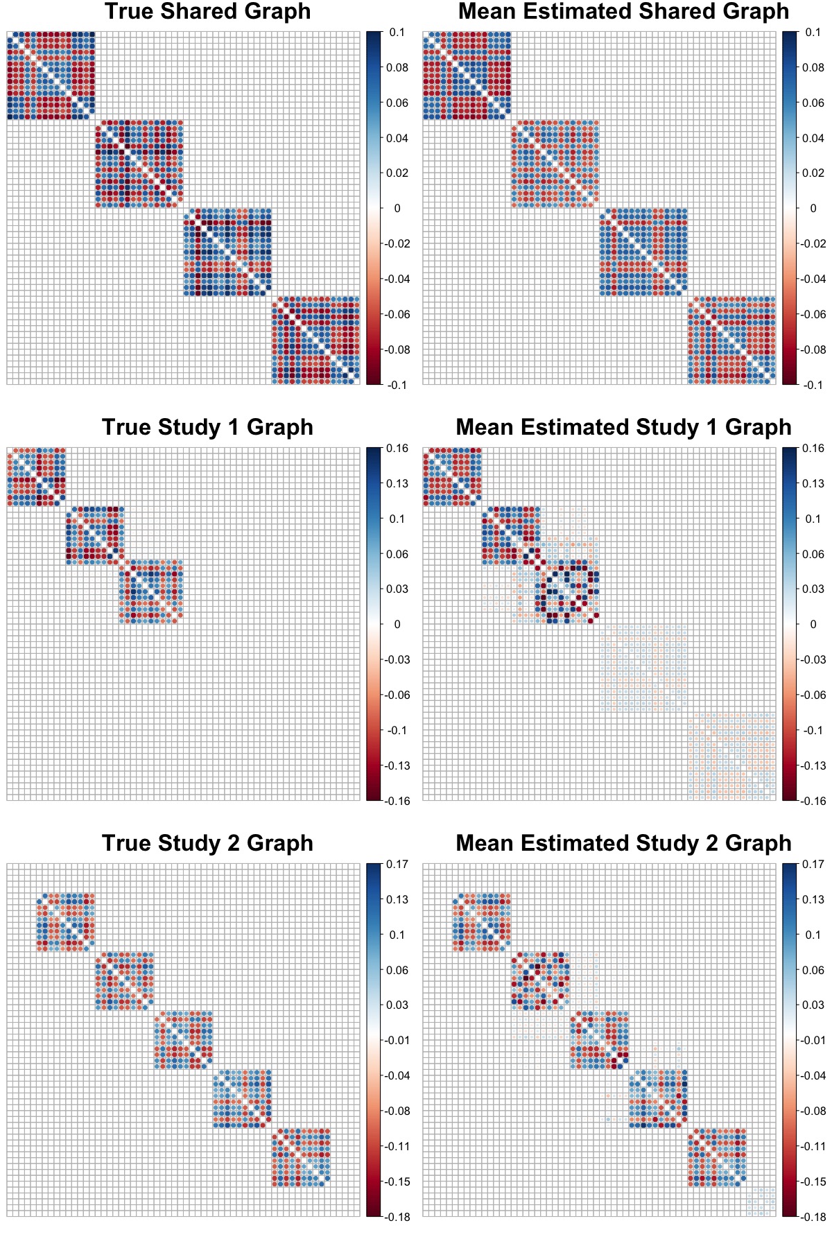
(b) Setting 4

Figure 3: Mean estimated GGM adjacency matrices across 100 simulated datasets for simulation setting 1 (baseline) and setting 4 (increased factor count).

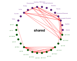
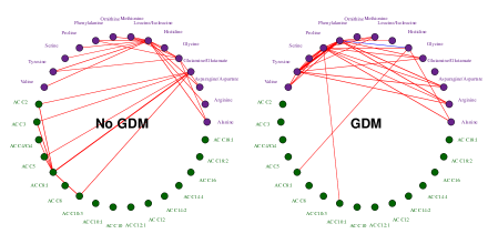
(a)

(b)

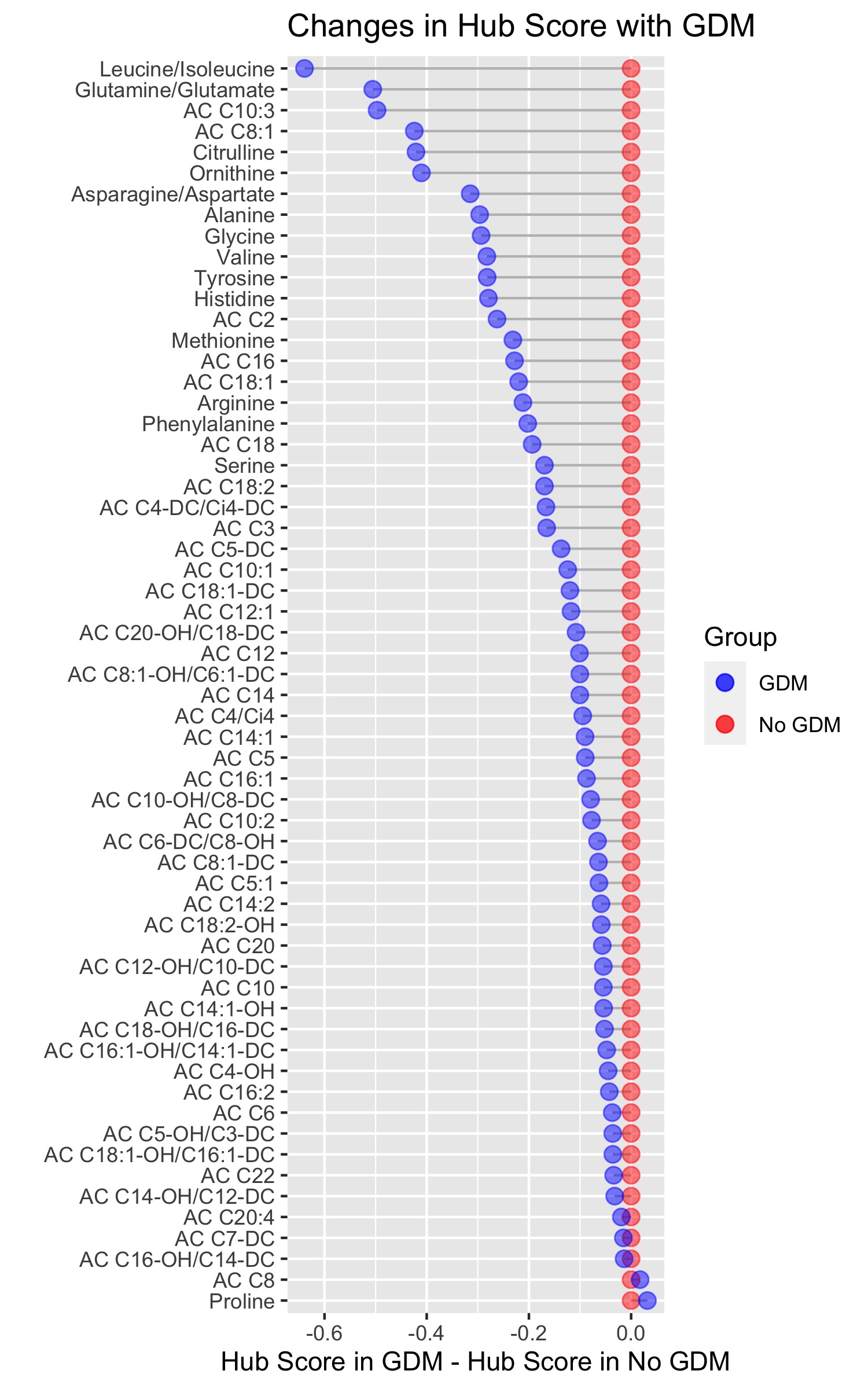
(c)

Figure 4: (a) MSFA-X estimated networks of conditional dependencies between metabolite changes in response to the oral glucose tolerance test. Green (purple) nodes indicate amino acids (acylcarnitines). Red (blue) edges indicate positive (negative) partial correlations. Edge width is proportional to the magnitude of the partial correlation. (b-c) Hub score of metabolites in the networks of women with GDM (blue) and without GDM (red). In (b), metabolites are ordered by hub score in the network of women without GDM. In (c), metabolites are ordered by difference in hub score relative to the hub score among women without GDM.

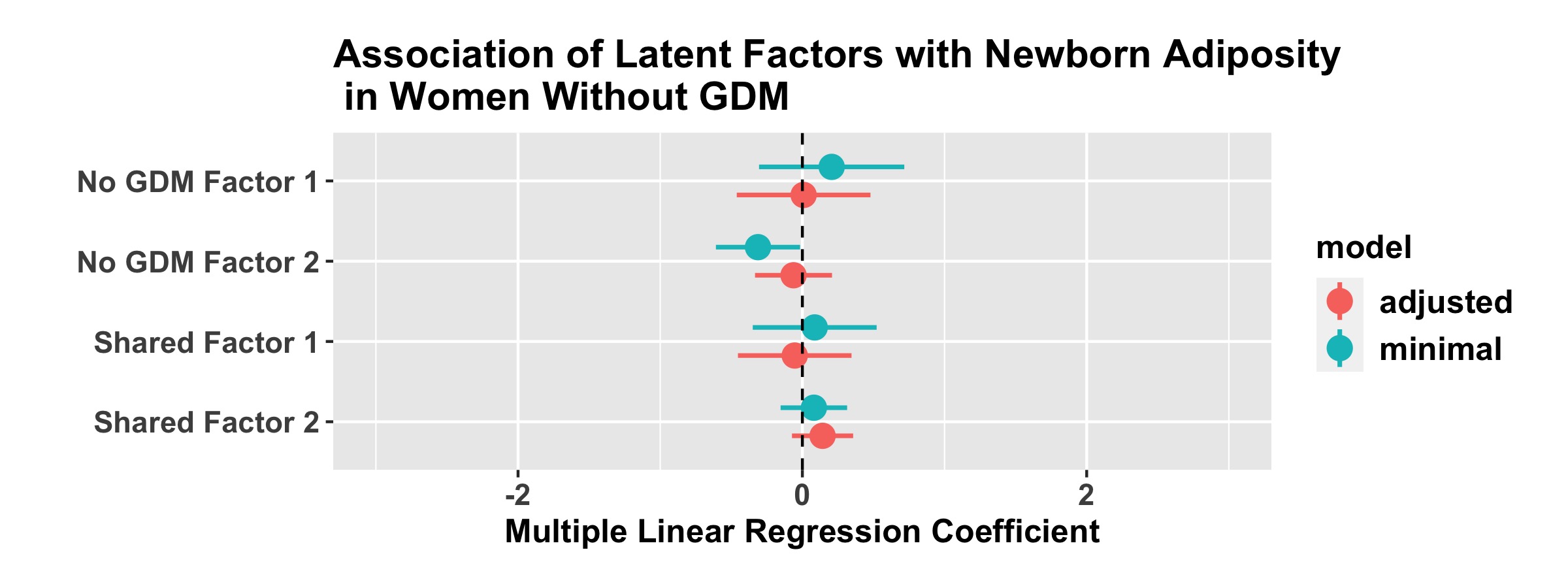
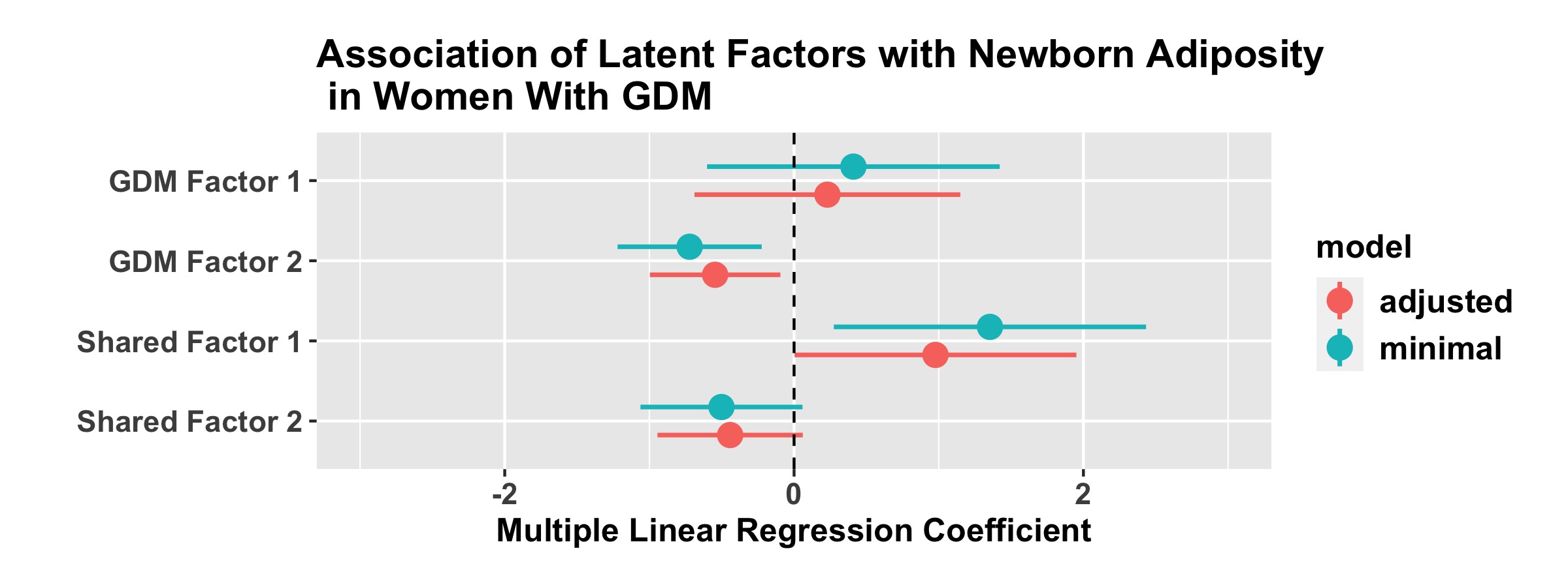
Figure 5: Latent variables learned by MSFA are associated with newborn adiposity in infants born to women with gestational diabetes.

The median and 95% quantile interval for the matrix RV coefficient between the estimated and true network in simulation settings 1,2,4,7, and 10 are shown in Table LABEL:tab:mrv. Results for the remaining settings and error metrics are presented in the Supplement (Supplementary Tables 5-7; Supplementary Figures 1-3). Visual inspection of the matrices estimated with MSFA-X shows the general structure of the GGM adjacency matrix was qualitatively well-recovered (Figure 3; Supplementary Figures 4-11). Together, these results suggest that MSFA-X can recover graphical structures induced by latent variables and outperform standard methods, despite identifiability limitations.

4 Application to the Hyperglycemia and Adverse Pregnancy Outcomes Study

The Hyperglycemia and Adverse Pregnancy Outcomes (HAPO) study is an international prospective cohort study investigating the relationship between maternal glucose metabolism and newborn outcomes among 25,505 mother-newborn pairs [10]. Details of the study have been previously described [10, 7]. Briefly, fasting plasma metabolomic profiles of the mothers were obtained prior to the administration of an oral glucose tolerance test (OGTT) near 28 weeks gestation and one hour after glucose intake [15, 16]. Targeted and untargeted metabolomic profiling was conducted as described by Kadakia et al. (2019); in this application, we use 60 targeted metabolites from these profiles [15] collected from a subset of 3463 of these participants comprised by $n=2887$ women without GDM and $n=576$ women with GDM. We apply MSFA-X to model shared and disease-specific conditional dependencies in glucose response based on changes from fasting metabolite levels to 1-hr post-glucose intake levels. For details of metabolite preprocessing and covariate adjustment, we refer the reader to Supplementary Section 2.1.

MSFA-X identified 2 shared factors, 2 study-specific factors for women without GDM, and 2 study-specific factors for women with GDM (Supplementary Figure 12). Thresholded shared and study-specific GGMs are shown in Figure 4(a), with thresholding based on based on a significance test of Fisher-transformed partial correlation coefficients (Supplementary Section 2.2). The shared network has two interesting connected components. One connected component contains the amino acids (AAs) along with three long-chain acylcarnitines (ACs; AC C18:1, AC C18:2, and AC C16). The second connected component contains several short- and medium-chain ACs, with the majority of edges connecting the medium-chain ACs. In the study-specific networks, edge patterns clearly identify differences in metabolism after glucose uptake between women with and without GDM. Among women without GDM, leucine/isoleucine and glutamine/glutamate are highly connected nodes, with glutamine/glutamate serving as a connector between the AAs and the short- and medium-chain ACs. AC C8:1 exhibits conditional associations with several short-chain ACs (AC C2, AC C3, AC C4/Ci4, AC C5). In contrast, leucine/isoleucine and glutamine/glutamate have much smaller degree in the GDM network, and glutamine/glutamate does not provide a bridge between AAs and ACs. Other AA patterns also differ: proline is more highly connected among women with GDM, and phenylalanine and tyrosine exhibit a strong conditional association. Conducting the same analysis with the graphical lasso benchmark showed that the benchmark was unable to disentangle these patterns between the two conditions (Supplementary Figure 13, 14).

We also conducted a quantitative analysis on the unthresholded networks by analyzing hub score. Hub score is an eigenvector-based measure of node centrality; a higher hub score indicates a node has more authority in the network [17]. Using the hub_score function of the igraph R package, we compared hub score in women with and without GDM (Figure 4(b), Figure 4(c)). This analysis recapitulates the finding of lower involvement of leucine/isoleucine and glutamine/glutamate in the network of women with GDM compared to women without GDM, as well as the observation of lower connectivity of AC C10:3 and AC C8:1 in women with GDM.

Because the sample sizes between the two groups in this application are substantially different (N=576 women with GDM vs. N=2887 women without GDM), our approach had higher power to detect network edges in the shared network and the non-GDM network than in the GDM network. To gain further confidence that the differences we observed between women with and without GDM were not simply due to the difference in sample size and power, we conducted a sensitivity analysis in which we downsampled the number of women without GDM to balance the sample, observing similar results (Supplementary Section 2.5). When conducting factor analysis, it is possible to find statistically relevant factors that do not carry practical meaning in the context of the problem. One way to validate context-specific relevancy is by associating the factors with an outcome of interest. In the context of the HAPO Study, one such outcome is newborn adiposity. Newborn adiposity is an important risk factor associated with childhood overweight[30]. As a final investigation in the HAPO application, we validated our factors by estimating their association with newborn adiposity.

For infants born to women participating in the HAPO Study, newborn adiposity was assessed by the sum of three skinfold measurements (“newborn sum of skinfolds”) as previously described [3]. Catalano et al. (2012) showed that gestational diabetes was associated with the newborn sum of skinfolds in the HAPO Study [3]. In this spirit, we proceeded to validate our latent factors by modeling the association between the newborn sum of skinfolds and the six factors identified by MSFA. We assigned a factor score for each individual in the study by projecting each individual’s vector of metabolite ratios $X^{i}=(X^{(i)}_{1},\dots,X^{(i)}_{60})$ onto each factor. For a factor $F=(F_{1},\dots,F_{60})$, this projection is calculated as:

$$proj_{F}(X^{i})=\frac{\sum_{j=1}^{60}F_{j}X^{(i)}_{j}}{\sqrt{\sum_{j=1}^{60}F_{j}^{2}}}$$ (11)

Larger values of $proj_{F}(X^{i})$ indicate higher colinearity of participant $i$’s metabolite profile with factor $F$. For women without GDM, projections were calculated onto the two shared factors $\Phi_{1}$ and $\Phi_{2}$ and the two non-GDM factors $\Lambda_{11}$ and $\Lambda_{12}$. For women with GDM, projections were calculated onto the two shared factors $\Phi_{1}$ and $\Phi_{2}$ and the two GDM factors $\Lambda_{21}$ and $\Lambda_{22}$. We then used multiple linear regression to regress the log sum of skinfolds onto these projections. Figure 5 shows the resulting associations. While none of the latent factors are significant in women without GDM, the first shared factor $\Phi_{1}$ and the second latent factor $\Lambda_{22}$ are both significantly associated with the log sum of skinfolds among the women with GDM ($\Phi_{1}$: $p=0.014$, 95% CI: $[0.275,2.433]$; $\Lambda_{22}$: $p=0.005$, 95% CI: $[-1.220,=0.224]$). These associations persist after adjusting for mean arterial pressure, BMI, age, and maternal height at the time of the OGTT, neonatal sex, gestational age at delivery, fasting plasma glucose, ancestry group, and storage time of the sample ($\Phi_{1}$: $p=0.050$, 95% CI: $[0.003,1.951]$; $\Lambda_{22}$: $0.018$, 95% CI: $[-0.997,-0.095]$). These results provide evidence for the context-specific relevance of the factors identified by MSFA in this application.

5 Discussion

The problem of comparing networks across multiple studies or conditions is often considered under the umbrella term of differential network analysis. Typical differential network analysis methods for GGMs do not focus on deconvoluting the shared and study-specific signal, but either on (i) estimating a GGM for each study which contains both signals or (ii) directly estimating the differential network between studies [25]. While these methods can produce accurate maps of conditional dependencies present in each study, they are not designed to allow the user to separate the shared and study-specific contributions to these dependencies. In contrast, MSFA-X accomplishes exactly this goal, providing a distinctive and interpretable perspective. MSFA-X is able to recover shared and study-specific conditional independence patterns (GGMs) and outperform a naive benchmark based on the graphical lasso.

MSFA-X has important limitations. First, factor analysis can be a restrictive method due to the numerous assumptions made regarding normality and independence of factors and residual noise, and MSFA-X is no exception. Copula methods such as the nonparanormal transformation have been widely used to facilitate the application of GGMs to non-normally distributed data, and we propose such approaches could also be applied to MSFA-X[20]. Future work could model correlated residuals by allowing different matrix structures for $\bm{\Gamma}$ and $\mathbf{H}_{s}$. For example, van Kesteren and Kievit (2021) present an open-source framework for modeling correlated residuals in the context of exploratory factor analysis in neuroscience [29]. A similar approach could be applied to MSFA-X [29]. Second, MSFA-X is limited in that it is a likelihood-based method with a non-identifiable likelihood. Our approach determines a region of non-identifiability and selects an estimate at the center of this region, meaning the error in these parameter estimates is bounded: we cannot be further off than the longest distance from the center of this region to its border. However, $\bm{\Gamma}$ and $\mathbf{H}_{s}$ are not the final estimands of interest in this problem; rather, we are trying to estimate the shared precision matrix $\hat{\Theta}_{MSFA-X}^{shared}=(\Phi\Phi^{T}+\Gamma)^{-1}$ and the study-specific precision matrices $\hat{\Theta}_{MSFA-X}^{study;s}=(\Lambda_{s}\Lambda_{s}^{T}+\mathbf{H}_{s})^{-1}$. Future work could explore how the bounded error in the estimation of $\bm{\Gamma}$ and $\mathbf{H}_{s}$ propagates to these latter estimands. Closed-form expressions for inverses of sums of matrices may prove useful; several previous works specifically address matrix inversion error [23, 19]. In our simulation studies, the relative error of MSFA-X was similar across a broad range of simulation studies, suggesting that such a bound does exist and could potentially be identified in closed form. A third limitation of MSFA-X is that, in contrast to the graphical lasso, it does not produce precision matrix estimates with exact zeros. This means that thresholding is required in order to produce a GGM that is not a completely connected graph. It would be interesting to explore regularization methods with structural specifications that could produce exact zeros in the factor loadings matrices and, consequently, sparse GGMs that do not require thresholding. Finally, MSFA-X, like all factor analysis methods, requires estimation of the number of factors. Our simulation study demonstrates that the accurate estimation of this quantity is an important part of accurate GGM estimation itself. We correctly identified the number of factors in many cases for small numbers of factors using our CNG-based approach, but our method does not work as well for settings with $>2$ factors per study. Future work is needed here, especially for high-dimensional biological data which are likely to have many factors.

MSFA-X is a tool for researchers to disentangle shared and study-specific network signals when working with data across multiple studies or conditions. This is a unique perspective compared to many existing methods for differential network analysis that do not deconvolute shared and study-specific signals. MSFA-X will assist researchers in gaining new insights into the direct dependencies underlying multi-study data, leading to improved understanding of complex biological function. The MSFA-X method is available as an extension of the R package MSFA [5] at https://github.com/katehoffshutta/MSFA.

6 Acknowledgments

The authors wish to acknowledge Nathan P. Gill for his valuable input to early conversations on the method. We gratefully acknowledge the participants of the HAPO Study. Research reported in this paper was supported by the National Heart, Lung, and Blood Institute of the National Institutes of Health under award number 1R01LM013444-01. The content is solely the responsibility of the authors and does not necessarily represent the official views of the National Institutes of Health.

Figure 1: An illustration of the covariance decomposition implied by the MSFA-X model formulation for $S=2$ studies on $p=12$ predictors.

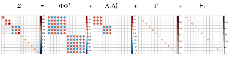
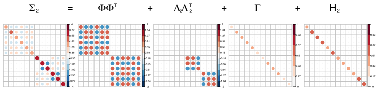
(a) Under the MSFA-X model formulation, the covariance matrix of the data in the $s^{th}$ study can be decomposed as $\bm{\Sigma}_{s}=\bm{\Phi}\bm{\Phi}^{\top}+\bm{\Lambda}_{s}\bm{\Lambda}_{s}^{\top}+\bm{\Gamma}+\mathbf{H}_{s}$. Here, we show the decomposition of simulated data. Our goal is to recover this decomposition for a given input dataset.

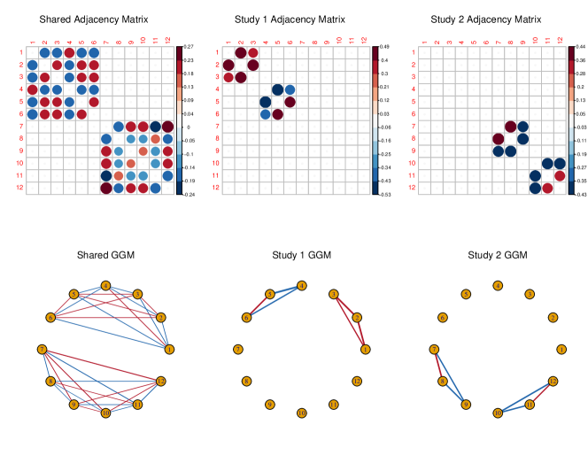
(b) The shared and study-specific precision matrices are shown here. Left, ($\bm{\Phi}\bm{\Phi}^{\top}+\bm{\Gamma})^{-1}$; center, $(\bm{\Lambda}_{1}\bm{\Lambda}_{1}^{\top}+\mathbf{H}_{1})^{-1}$; right, $(\bm{\Lambda}_{2}\bm{\Lambda}_{2}^{\top}+\mathbf{H}_{2})^{-1}$. Estimating these matrices allows us to estimate the corresponding shared and study-specific GGMs. Red indicates positive values; blue, negative. Edge width in graphs is proportional to magnitude of partial correlation between two variables.

Figure 2: A visual of the region of non-identifiability for one predictor in the case of three studies ($S=3$). $\gamma$: true, unknown shared noise for this predictor; $\hat{\psi}_{s}$: estimated overall noise; $\hat{\gamma}$: estimated shared noise; $\hat{\eta}_{s}$: estimated study-specific noise; $\Delta\gamma$: error in estimating $\gamma$.

(a) Setting 1

Table 1: Simulation study design.

Setting	Description	# Studies ($S$)	Sample Sizes ($n_{s}$)	Predictors ($p$)	Shared Factors $(k)$	Study-Specific Factors ($j_{s}$)	Noise $(\Gamma,\mathbf{H}_{s})$	Exact Zeros
1	Baseline	2	1600, 1600	60	2	2,2	equal	Yes
2	Change # of predictors	2	1600, 1600	12	2	2,2	equal	Yes
3	Change # of studies	4	1600, 1600, 1600, 1600	60	2	2,2,2,2	equal	Yes
4	Change # of factors	2	1600, 1600	60	4	3,5	equal	Yes
5	Small sample size	2	250, 250	60	2	2,2	equal	Yes
6	Unequal sample size	2	1600, 250	60	2	2,2	equal	Yes
7	Unequal noise	2	1600, 1600	60	2	2,2	$\Gamma>\mathbf{H}_{s}$	Yes
8	Unequal noise	2	1600, 1600	60	2	2,2	$\mathbf{H}_{s}>\Gamma$	Yes
9	Not true zeros	2	1600, 1600	60	2	2,2	equal	No
10	Mimic HAPO application	2	2887, 576	60	2	2,2	equal	No

Table 2: Matrix RV coefficients for simulation settings 1,2,4,7, and 10. A higher value of the matrix RV coefficient corresponds to better estimation of the gold standard matrix in the simulation. The maximum value for the RV coefficient is 1. Est. Fac. refers to a simulation in which we estimated the number of factors using our CNG-based method. True Fac. refers to a simulation in which we used the true number of factors from the known data generating process.

Method	Setting	Study	Median	2.5th percentile	97.5th percentile
glasso	Setting 1	Shared	0.5412	0.5396	0.5428
MSFA-X: Est. Fac.	Setting 1	Shared	0.9946	0.9939	0.9955
MSFA-X: True Fac.	Setting 1	Shared	0.9946	0.9939	0.9955
glasso	Setting 1	Study 1	0.0135	0.0125	0.0145
MSFA-X: Est. Fac.	Setting 1	Study 1	0.9929	0.9891	0.995
MSFA-X: True Fac.	Setting 1	Study 1	0.9929	0.9891	0.995
glasso	Setting 1	Study 2	0.0149	0.0142	0.0156
MSFA-X: Est. Fac.	Setting 1	Study 2	0.9943	0.9892	0.9963
MSFA-X: True Fac.	Setting 1	Study 2	0.9943	0.9892	0.9963
glasso	Setting 2	Shared	0.6589	0.651	0.6663
MSFA-X: Est. Fac.	Setting 2	Shared	0.6755	0.3687	0.9852
MSFA-X: True Fac.	Setting 2	Shared	0.9674	0.5375	0.9958
glasso	Setting 2	Study 1	0.0479	0.0351	0.0616
MSFA-X: Est. Fac.	Setting 2	Study 1	0.8375	0.2649	0.987
MSFA-X: True Fac.	Setting 2	Study 1	0.9124	0.1079	0.9887
glasso	Setting 2	Study 2	0.0645	0.0549	0.0735
MSFA-X: Est. Fac.	Setting 2	Study 2	0.8677	0.6018	0.9733
MSFA-X: True Fac.	Setting 2	Study 2	0.9633	0.5042	0.9942
glasso	Setting 4	Shared	0.5122	0.5092	0.5153
MSFA-X: Est. Fac.	Setting 4	Shared	0.99	0.7002	0.9933
MSFA-X: True Fac.	Setting 4	Shared	0.9927	0.9918	0.9937
glasso	Setting 4	Study 1	0.1009	0.0969	0.1046
MSFA-X: Est. Fac.	Setting 4	Study 1	0.781	0.6754	0.8407
MSFA-X: True Fac.	Setting 4	Study 1	0.9877	0.9835	0.9909
glasso	Setting 4	Study 2	0.0795	0.0749	0.0833
MSFA-X: Est. Fac.	Setting 4	Study 2	0.9133	0.8439	0.9917
MSFA-X: True Fac.	Setting 4	Study 2	0.9914	0.9882	0.9936
glasso	Setting 7	Shared	0.5424	0.5412	0.5442
MSFA-X: Est. Fac.	Setting 7	Shared	0.9989	0.9987	0.9992
MSFA-X: True Fac.	Setting 7	Shared	0.9989	0.9987	0.9992
glasso	Setting 7	Study 1	0.015	0.0145	0.0158
MSFA-X: Est. Fac.	Setting 7	Study 1	0.9852	0.9811	0.9879
MSFA-X: True Fac.	Setting 7	Study 1	0.9852	0.9811	0.9879
glasso	Setting 7	Study 2	0.0153	0.0147	0.0159
MSFA-X: Est. Fac.	Setting 7	Study 2	0.9912	0.9868	0.9937
MSFA-X: True Fac.	Setting 7	Study 2	0.9912	0.9868	0.9937
glasso	Setting 10	Shared	0.4172	0.4135	0.4211
MSFA-X: Est. Fac.	Setting 10	Shared	0.9015	0.2351	0.996
MSFA-X: True Fac.	Setting 10	Shared	0.9959	0.9954	0.9965
glasso	Setting 10	Study 1	0.1151	0.1127	0.1171
MSFA-X: Est. Fac.	Setting 10	Study 1	0.4937	0.3065	0.8582
MSFA-X: True Fac.	Setting 10	Study 1	0.9959	0.995	0.9966
glasso	Setting 10	Study 2	0.0627	0.0533	0.07
MSFA-X: Est. Fac.	Setting 10	Study 2	0.769	0.5815	0.8414
MSFA-X: True Fac.	Setting 10	Study 2	0.9933	0.9886	0.9961

References

- Altenbuchinger et al. [2020] Michael Altenbuchinger, Antoine Weihs, John Quackenbush, Hans Jörgen Grabe, and Helena U Zacharias. Gaussian and mixed graphical models as (multi-) omics data analysis tools. Biochimica et Biophysica Acta (BBA)-Gene Regulatory Mechanisms, 1863(6):194418, 2020.
- Casella and Berger [2002] George Casella and Roger L Berger. Statistical inference, volume 2. Duxbury Pacific Grove, CA, 2002.
- Catalano et al. [2012] Patrick M Catalano, H David McIntyre, J Kennedy Cruickshank, David R McCance, Alan R Dyer, Boyd E Metzger, Lynn P Lowe, Elisabeth R Trimble, Donald R Coustan, David R Hadden, et al. The hyperglycemia and adverse pregnancy outcome study: associations of gdm and obesity with pregnancy outcomes. Diabetes care, 35(4):780–786, 2012.
- Danaher et al. [2014] Patrick Danaher, Pei Wang, and Daniela M Witten. The joint graphical lasso for inverse covariance estimation across multiple classes. Journal of the Royal Statistical Society. Series B, Statistical methodology, 76(2):373, 2014.
- De Vito et al. [2019] Roberta De Vito, Ruggero Bellio, Lorenzo Trippa, and Giovanni Parmigiani. Multi-study factor analysis. Biometrics, 75(1):337–346, 2019.
- Friedman et al. [2008] Jerome Friedman, Trevor Hastie, and Robert Tibshirani. Sparse inverse covariance estimation with the graphical lasso. Biostatistics, 9(3):432–441, 2008.
- Group et al. [2002] HAPO Study Cooperative Research Group et al. The hyperglycemia and adverse pregnancy outcome (hapo) study. International Journal of Gynecology & Obstetrics, 78(1):69–77, 2002.
- Guo et al. [2011] Jian Guo, Elizaveta Levina, George Michailidis, and Ji Zhu. Joint estimation of multiple graphical models. Biometrika, 98(1):1–15, 2011.
- Ha et al. [2015] Min Jin Ha, Veerabhadran Baladandayuthapani, and Kim-Anh Do. Dingo: differential network analysis in genomics. Bioinformatics, 31(21):3413–3420, 2015.
- HAPO Study Cooperative Research Group [2008] HAPO Study Cooperative Research Group. Hyperglycemia and adverse pregnancy outcomes. New England Journal of Medicine, 358(19):1991–2002, 2008.
- Huang et al. [2018] Justin K Huang, Daniel E Carlin, Michael Ku Yu, Wei Zhang, Jason F Kreisberg, Pablo Tamayo, and Trey Ideker. Systematic evaluation of molecular networks for discovery of disease genes. Cell systems, 6(4):484–495, 2018.
- Ideker and Nussinov [2017] Trey Ideker and Ruth Nussinov. Network approaches and applications in biology, 2017.
- Jöreskog [1967] Karl G Jöreskog. Some contributions to maximum likelihood factor analysis. Psychometrika, 32(4):443–482, 1967.
- Jöreskog [1971] Karl G Jöreskog. Simultaneous factor analysis in several populations. Psychometrika, 36(4):409–426, 1971.
- Kadakia et al. [2019a] Rachel Kadakia, Michael Nodzenski, Octavious Talbot, Alan Kuang, James R Bain, Michael J Muehlbauer, Robert D Stevens, Olga R Ilkayeva, Sara K O’Neal, Lynn P Lowe, et al. Maternal metabolites during pregnancy are associated with newborn outcomes and hyperinsulinaemia across ancestries. Diabetologia, 62(3):473–484, 2019a.
- Kadakia et al. [2019b] Rachel Kadakia, Octavious Talbot, Alan Kuang, James R Bain, Michael J Muehlbauer, Robert D Stevens, Olga R Ilkayeva, Lynn P Lowe, Boyd E Metzger, Christopher B Newgard, et al. Cord blood metabolomics: association with newborn anthropometrics and c-peptide across ancestries. The Journal of Clinical Endocrinology & Metabolism, 104(10):4459–4472, 2019b.
- Kleinberg et al. [1998] Jon M Kleinberg et al. Authoritative sources in a hyperlinked environment. In SODA, volume 98, pages 668–677. Citeseer, 1998.
- Lauritzen [1996] Steffen L Lauritzen. Graphical models, volume 17. Clarendon Press, 1996.
- Lefebvre et al. [2000] M Lefebvre, RK Keeler, R Sobie, and J White. Propagation of errors for matrix inversion. Nuclear Instruments and Methods in Physics Research Section A: Accelerators, Spectrometers, Detectors and Associated Equipment, 451(2):520–528, 2000.
- Liu et al. [2009] Han Liu, John Lafferty, and Larry Wasserman. The nonparanormal: Semiparametric estimation of high dimensional undirected graphs. Journal of Machine Learning Research, 10(10), 2009.
- Lopes and West [2004] Hedibert Freitas Lopes and Mike West. Bayesian model assessment in factor analysis. Statistica Sinica, pages 41–67, 2004.
- Loscalzo [2017] Joseph Loscalzo. Network medicine. Harvard University Press, 2017.
- Miller [1981] Kenneth S Miller. On the inverse of the sum of matrices. Mathematics magazine, 54(2):67–72, 1981.
- Robert and Escoufier [1976] Paul Robert and Yves Escoufier. A unifying tool for linear multivariate statistical methods: the rv-coefficient. Journal of the Royal Statistical Society: Series C (Applied Statistics), 25(3):257–265, 1976.
- Shojaie [2021] Ali Shojaie. Differential network analysis: A statistical perspective. Wiley Interdisciplinary Reviews: Computational Statistics, 13(2):e1508, 2021.
- Smilde et al. [2009] Age K Smilde, Henk AL Kiers, Sabina Bijlsma, CM Rubingh, and MJ Van Erk. Matrix correlations for high-dimensional data: the modified rv-coefficient. Bioinformatics, 25(3):401–405, 2009.
- Stewart [1969] GW Stewart. On the continuity of the generalized inverse. SIAM Journal on Applied Mathematics, 17(1):33–45, 1969.
- Tantardini et al. [2019] Mattia Tantardini, Francesca Ieva, Lucia Tajoli, and Carlo Piccardi. Comparing methods for comparing networks. Scientific reports, 9(1):1–19, 2019.
- Van Kesteren and Kievit [2021] Erik-Jan Van Kesteren and Rogier A Kievit. Exploratory factor analysis with structured residuals for brain network data. Network Neuroscience, 5(1):1–27, 2021.
- Winter et al. [2010] Jonathan David Winter, Patricia Langenberg, and Scott D Krugman. Newborn adiposity by body mass index predicts childhood overweight. Clinical pediatrics, 49(9):866–870, 2010.
- Zhao et al. [2014] Sihai Dave Zhao, T Tony Cai, and Hongzhe Li. Direct estimation of differential networks. Biometrika, 101(2):253–268, 2014.