Unsupervised particle sorting for cryo-EM using probabilistic PCA

Abstract

Single-particle cryo-electron microscopy (cryo-EM) is a leading technology to resolve the structure of molecules. Early in the process, the user detects potential particle images in the raw data. Typically, there are many false detections as a result of high levels of noise and contamination. Currently, removing the false detections requires human intervention to sort the hundred thousands of images. We propose a statistically-established unsupervised algorithm to remove non-particle images. We model the particle images as a union of low-dimensional subspaces, assuming non-particle images are arbitrarily scattered in the high-dimensional space. The algorithm is based on an extension of the probabilistic PCA framework to robustly learn a non-linear model of union of subspaces. This provides a flexible model for cryo-EM data, and allows to automatically remove images that correspond to pure noise and contamination. Numerical experiments corroborate the effectiveness of the sorting algorithm.

Index Terms—  Unsupervised learning, single-particle cryo-EM, probabilistic PCA, expectation-maximization

1   Introduction

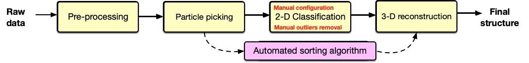
Fig. 1: A typical data processing pipeline for single-particle cryo-EM. The main contribution of this work is the fully automated sorting block, aiming to replace the need of an expert practitioner involved in the sorting step.

Single-particle cryo-electron microscopy (cryo-EM) is an emerging technology to determine the structure of molecules. In the cryo-EM process, the acquired “raw data” image, called a micrograph, contains a few dozens of 2-D tomographic particle projection images with unknown random orientations and locations. The micrograph suffers from low signal-to-noise ratio (SNR), as low as $\frac{1}{100}$. Typically, it also contains undesired contamination. For the purpose of this paper, the pixels in a micrograph can be broadly divided into three categories: regions of particles with additive noise, regions of contamination, and regions of noise only.

During the cryo-EM workflow, particle images are detected and extracted from micrographs in a process called particle picking [1, 2]. The extracted images are the individual particles within each micrograph. If only particles were picked, the images chosen by the particle picker would have been used to construct the 3-D molecular structure. Figure 1 illustrates a schematic sequence of computational steps typically used to convert the raw data into 3-D molecular structures. While many particle picking algorithms were developed, e.g.,  [3, 4, 5], due to very low SNR levels they result in contamination and pure noise images picked along with the particle images. Typical images chosen by a picking algorithm can be seen in Figure 2.

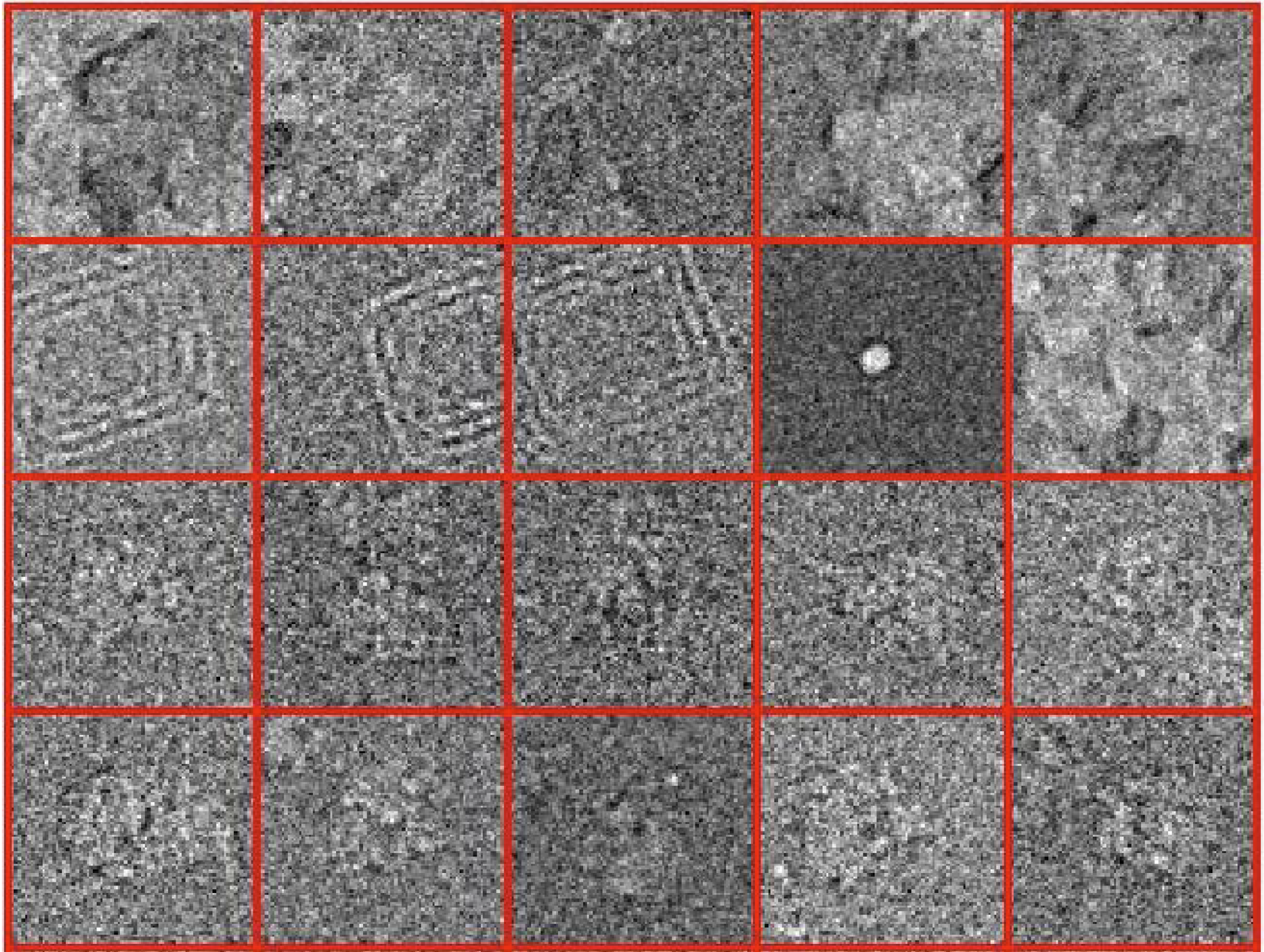
Fig. 2: Highest scoring images by the KLT picker [5] on Plasmodium falciparum 80S ribosome [6]. Two bottom rows consist of particle images, while the others are contamination images.

A common approach to remove non-particle images, called “2-D classification,” is semi-automatic and involves an expert practitioner; it relies heavily on subjective criteria that are neither consistent nor reproducible among different users. We propose an automatic and statistically-established unsupervised algorithm to remove non-particle images from the data. Specifically, we assume that all particle images approximately lie on a union of subspaces, whereas the non-particle images are scattered in the high-dimensional space. Similar parsimonious models are ubiquitous in many signal processing tasks, and specifically in different stages of the cryo-EM computational pipeline [7, 8]. The main computational tool in this work is an extension of principal component analysis (PCA). PCA has been applied to cryo-EM data for several tasks [7, 9]. However, PCA is limited since it learns a single subspace. We build on a maximum likelihood formulation, called probabilistic PCA (PPCA) [10, 11, 12]. In particular, we iteratively estimate the union of subspaces using an expectation-maximization (EM) algorithm, while sorting out images that do not lie on the subspaces.

PPCA offers several attractive advantages over PCA. First, PPCA can be readily extended to multiple subspaces, leading to a nonlinear flexible mixture model. Second, we work in the dimension of the problem (i.e., the number of parameters that define the sought subspaces) in contrast to standard PCA that requires estimating the full covariance matrix.

2   Existing particle sorting solutions

Several algorithms have been proposed to automate the particle sorting step. In general, such algorithms can be divided into two main groups: semi-automatic and automatic. Since a typical cryo-EM dataset after particle picking contains hundreds thousands of images, it is unreasonable to visually inspect each one of them. Thus, in a typical semi-automated sorting, the images are clustered based on their similarity using a 2-D classification tool [13]. An expert then visually inspects representative images of the clusters and discards uninformative ones, as demonstrated in Figure 3.

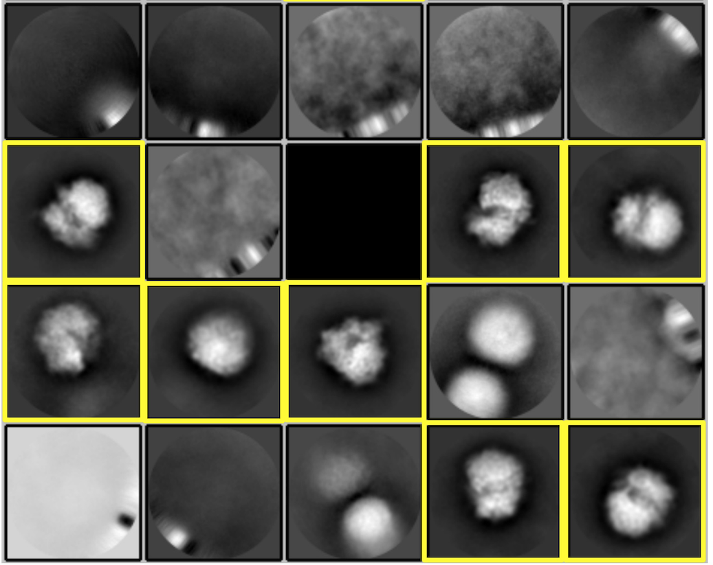
Fig. 3: The current practice to remove non-particle images begins with clustering similar images, a procedure called 2-D classification. The figure shows the results of RELION’s 2-D classification tool [3] on the Plasmodium falciparum 80S ribosome dataset [6], picked using the KLT picker [5]. An expert manually chooses the particle classes (marked in yellow). Then, the user re-runs the 2-D classification algorithm on the images associated with the selected classes. This step is usually done multiple times to reach satisfying results.

Almost all cryo-EM users remove the non-particle images using 2-D classification, but a few automated methods have been proposed. One approach uses a statistical model of mixture of two Gaussians for the distribution of scores assigned during refinement [14]; this method relies on the availability of a satisfying initial 3-D model of the investigated molecule.. Unfortunately, often, a reliable initial model is unavailable. Another approach uses transfer learning techniques to sort cryo-EM images [15]. This method requires a labeled dataset, thus it reduces the amount of experts’ manual work but it still depends the user’s subjective viewing point. Another deep learning approach takes multiple picking algorithms’ output and consolidates their results; this is time-consuming and demanding on computational resources [16]. None of the existing works are unsupervised and self-sufficient. In contrast, our proposed method does not require any human intervention nor professional expertise involved.

3   Unsupervised particle sorting

Our approach is based on a nonlinear mixture model composed of factors of PPCA analyzers. Our proposed algorithm consists of two main ingredients. The first is the union of subspaces model and the EM algorithm that aims to estimate the subspaces. The second is the sorting method, which removes images that are distant from the learned union of subspaces.

We fuse these two tools into one sorting algorithm: given a set of images picked by some particle picking algorithm, our goal is to find a subset of the particle images, while removing the contamination images. The proposed EM method estimates the multiple subspaces simultaneously. As the EM algorithm is iterative, we concurrently sort out images which we consider “far” from the learned subspaces during the estimation process. Namely, we discard the images which are most likely not to originate from the subspaces. Discarding images during each iteration should improve the next learning iteration of subspaces, as the outliers—which do not lie on the subspaces—are discarded. Thus, we gain two birds with one stone. First, the estimation process is improved, assuming we removed outlier images (i.e., non-particle images). Second, we reduce the computational burden as the data set contains fewer images. A scheme of the algorithm is presented in Figure 4.

We begin by mathematically formulating the image generative model. Next, we explain how we estimate the sought subspaces via the EM algorithm. Ultimately, we present our approach for online sorting. Numerical results are deferred to the next section.

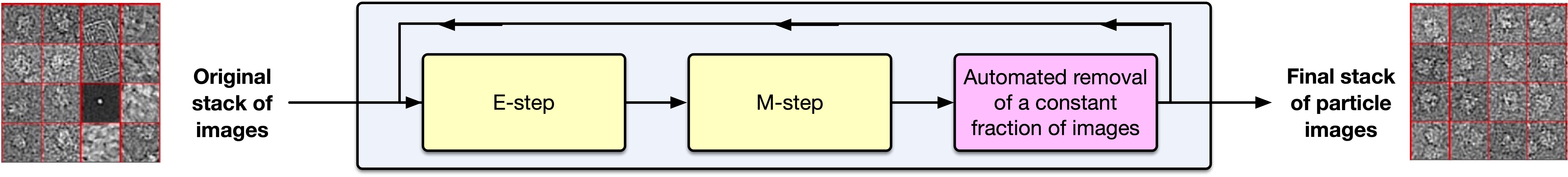
Fig. 4: Schematic view of the sorting procedure. The EM iterations alternate between performing an E-step and an M-step; every several iterations we remove a constant fraction of the stack of images.

3.1 Image formation model

We assume that the particle images lie in a low-dimensional (non-linear) union of $M$ unknown subspaces, whereas the non-particle images are arbitrarily scattered in the high $L$-dimensional space. Each image is assumed to originate from one of the subspaces. For subspace $1\leq m\leq M$, we define the mixture indicator variable $w_{m}\in{[0,1]}$, where $w_{m}=1$ when the image was generated by subspace $m$.

We assume to acquire $N$ image realizations drawn from the model $y=C_{w_{m}}x+\mu_{w_{m}}+\varepsilon,$ where $C_{1},\ldots,C_{M}\in\mathbb{R}^{L\times K}$ are matrices that span the sought subspaces, $\mu_{1},\ldots,\mu_{M}\in\mathbb{R}^{L\times 1}$ are mean vectors that are the centers of the subspaces, $K<<L$, and $x\in\mathbb{R}^{K\times 1}$ are the low-dimensional coefficients, lying in the union of subspaces, which are normally distributed with zero mean and unit covariance. The additive noise is normally distributed $\varepsilon\sim\mathcal{N}(0,\sigma^{2}I_{L})$. The vector $\pi=(\pi_{1},\ldots,\pi_{M})^{T}$ denotes a distribution of the particles over the $M$ subspaces so that $\pi_{m}=\text{p}(w_{m}=1)$, where $\text{p}(\cdot)$ denotes probability densities. Furthermore, $\varepsilon$, $w_{m}$ and $x$ are independent.

We are interested in estimating the model parameters and $\pi$, while $x_{1},\ldots,x_{N}$ are treated as nuisance variables. We also estimate the noise variance $\sigma^{2}$. Accordingly, the generative model reads $\text{p}(y)=\sum_{m=1}^{M}\int\text{p}(y|x,w_{m})\text{p}(x)\text{p}(w_{m})dx,$ with $x\sim\mathcal{N}(0,I_{K})$.

We use the prolate spheroidal wave functions (PSWFs) [17, 9] basis to reduce dimensionality of the input images, but other bases may be used instead. In the sequel, with a slight abuse of notation, we refer to the PSWF coefficients of the images as the images.

3.2 EM algorithm

Expectation-maximization (EM) is an iterative method to maximize the likelihood function of statistical models that include nuisance variables [18]. In our problem, given the observations $y_{1},\ldots,y_{N}$, we wish to estimate the subspaces’ parameters, the distribution over the subspaces, and the noise variance, that maximize the likelihood function. We denote all parameters by $\theta$. The nuisance variables of the model—namely, unknowns whose estimation is not the aim of the task—are the coefficients $x_{1},\ldots,x_{N}$ and the indicators $w_{m}$ associated with each measurement.

Let

$$\vspace{-3 mm}\theta_{t}=\left\{C_{1}^{(t)},...,C_{M}^{(t)},\mu_{1}^{(t)},\ldots,\mu_{M}^{(t)},\pi^{(t)},{\sigma^{2}}^{(t)}\right\}$$ (3.1)

be the estimate of the model parameters at the $t$-th EM iteration. At each EM iteration, we wish to maximize the expected complete log-likelihood, given by $Q(\theta|\theta_{t})=\mathbb{E}_{x,w|y,\theta_{t}}\left[\mathcal{L}(\theta;y,x,w)\right],$ where $\mathcal{L}(\theta;y,x,w)$ is the complete-data log-likelihood of the generative model. Explicitly, it is given, up to a constant, by

$$\vspace{-12 mm}Q(\theta|\theta_{t}) =\sum_{i=1}^{N}\sum_{m=1}^{M}\mathbb{E}_{x,w|y,\theta_{t}}[w_{m}\log{\text{p}(y_{i}|x_{i},w_{m})\text{p}(x_{i})}]$$

$$=-\frac{L}{2}\log{{\sigma^{2}}^{(t)}}-\frac{1}{2{\sigma^{2}}^{(t)}}\sum_{i,m}h_{i,m}\bigg{(}\|y_{i}-\mu_{m}^{(t)}\|^{2}$$

$$+\text{trace}({C_{m}^{(t)}}^{T}C_{m}^{(t)}\mathbb{E}[x_{i}x_{i}^{T}|y_{i},w_{m}])$$ (3.2)

$$+2(\mu_{m}^{(t)}-y_{i})^{T}C_{m}^{(t)}\mathbb{E}[x_{i}|y_{i},w_{m}]\bigg{)},\vspace{-10 mm}$$

where

$$\vspace{-2 mm}h_{i,m}=\mathbb{E}(w_{m}|y_{i}).$$ (3.3)

Each EM iteration consists of two steps. For the first step, the E-step, we calculate the expectations of the nuisance variables that appear in the Q function (3.2). It can be shown that

$$\mathbb{E}[x_{i}|y_{i},w_{m}]=B_{m}(y_{i}-\mu_{m}),$$ (3.4)

$$\mathbb{E}[x_{i}{x_{i}}^{T}|y_{i},w_{m}]=I_{K}-B_{m}C_{m}^{T}+B_{m}(y_{i}-\mu_{m})(y_{i}-\mu_{m})^{T}B_{m}^{T},\vspace{-8 mm}$$ (3.5)

where $B_{m}=C_{m}^{T}(C_{m}C_{m}^{T}+\sigma^{2}I_{L})^{-1}\in\mathbb{R}^{K\times L}.$

For the second step of the EM algorithm, the M-step, we maximize the expected log-likelihood, namely, solve $\theta^{(t+1)}=\operatorname*{argmax}_{\theta}Q(\theta|\theta_{t}),$ assuming the expectations of the nuisance variables are known. The maximum is attained as the solution of the linear system of equations:

$$\vspace{-5 mm}{C_{m}^{(t+1)}}= \left(\sum_{i}h_{i,m}(y_{i}-{\mu_{m}^{(t+1)}})\mathbb{E}[x_{i}^{T}|y_{i},w_{m}]\right)$$ (3.6)

$$\left(\sum_{i}h_{i,m}\mathbb{E}[x_{i}x_{i}^{T}|y_{i},w_{m}]\right)^{-1},\vspace{-8 mm}$$

$${\mu_{m}^{(t+1)}}=\frac{1}{N}\sum_{i}h_{i,m}(y_{i}-{C_{m}^{(t+1)}}\mathbb{E}[x_{i}|y_{i},w_{m}]),\vspace{-5 mm}$$ (3.7)

$${\sigma^{2}}^{(t+1)}= \frac{1}{L}\sum_{i,m}h_{i,m}^{(t)}(\|y_{i}-\mu_{m}^{(t+1)}\|^{2}$$

$$+\text{trace}(C_{m}^{T(t+1)}C_{m}^{(t+1)}\mathbb{E}[x_{i}x_{i}^{T}|y_{i},w_{m}])$$ (3.8)

$$+2(\mu_{m}^{T(t+1)}-y_{i}^{T})C_{m}^{(t+1)}\mathbb{E}[x_{i}|y_{i},w_{m}]).\vspace{-2 mm}$$

Table 1: Simulated data results of Section 4.1, $K_{\text{total}}=60$.

	Raw Data	1 Subspace	2 Subspaces	3 Subspaces	sPCA
% Particles	83.33	87.89	89.25	91.04	90.1
% Outliers	8.33	3.38	3.95	2.9	9.6
% Noise	8.33	8.73	6.8	6.06	0.84

3.3 Online sorting

Assuming the particle images lie in the learned subspaces, for an image $y_{i}\in\mathbb{R}^{L\times 1}$, and a subspace $C_{m}\in\mathbb{R}^{L\times K}$, the sorting factor is defined by

$$\text{SF}_{m}(y_{i})=\frac{\text{projection error}}{\text{projected energy}}=\frac{\|C_{m}C_{m}^{T}y_{i}-y_{i}\|_{\text{F}}^{2}}{\|C_{m}C_{m}^{T}y_{i}\|_{\text{F}}^{2}},\vspace{-3 mm}$$ (3.9)

where $C_{m}C_{m}^{T}y_{i}$ is the projection of $y_{i}$ onto the subspace spanned by $C_{m}$. A large value indicates the image is far from the subspace.

In practice, after every constant number of $P$ iterations of the EM algorithm, we calculate the SF for each pair of an image and a subspace, and sort the images by summing up the factor value for all subspaces (per image). Then, at every sorting step, we remove a constant fraction, denoted by $\alpha$, of the images in the stack. The algorithm is outlined in Algorithm 1.

4   Numerical Experiments

In this section, we describe numerical results on synthetic and experimental data sets. The code to reproduce all experiments is publicly available at https://github.com/giliw/particle_sorting.

4.1 Simulated cryo-EM data

We generated 50K tomographic projections of $71\times 71$ pixels of the 80S ribosome, available at the Electron Microscopy Data Bank (www.ebi.ac.uk/emdb/EMD-2275), using the ASPIRE package (www.spr.math.princeton.edu). We added additive white Gaussian noise, resulting in SNR = $\frac{1}{10}$. We added random small shifts to the images. We also added outlier images—representing contamination in the micrographs—modeled as random cuts of Matlab’s “camera-man” image, which were $8.33\%$ of the images. In addition, we added pure noise images which also comprised $8.33\%$ of the images. Throughout all the experiments, every $P=6$ EM iterations we sort out $\alpha=5\%$ of the images.

We run the unsupervised sorting algorithm with 1, 2 and 3 subspaces, where the total dimension was fixed to $K_{\text{total}}=60$. For example, when we estimated two subspaces, the dimension of each subspace was set to 30. We tested our sorting algorithm against a sorting algorithm based on steerable PCA (sPCA) [7]. This algorithm takes $K_{\text{total}}$ eigenimages of sPCA (corresponding to the largest eigenvalues), and then projects the images to that linear subspace. Finally, it sorts the reconstructed images based on the relative energy of the images with respect to the original images, and takes those with the highest value. We compare against this algorithm since it is a linear algorithm, and is based on a popular cryo-EM practice.

Table 1 presents the results. The original simulated images are referred to as “Raw Data”. We see that three subspaces were best at sorting out the outliers, improving the $83.333\%$ in the original dataset to $91.04\%$ particle images. Our numerical experiments indicate that more than three subspaces do not improve the results. Although sPCA seems to achieve a similar particle images percentage, it almost did not discard outlier images. In particular, we note that sPCA works well in removing the pure noise images, but this is a much easier problem that can be solved using standard statistical tests for detecting Gaussian noise, and is not the focus of this work.

Table 2: Sorted tagged EMPIAR-10028 dataset, $K_{\text{total}}=60$.

	Raw data	1 Subspace	2 Subspaces	3 Subspaces	sPCA
% Particles	97	97.75	98.2	97.9	97.45
% of the outliers sorted	-	31.82	45.45	36.36	22.73
$\#$ Images	742	667	667	667	667

Table 3: Sorted EMPIAR-10028 dataset, $K_{\text{total}}=60$.

	Raw data	1 Subspace	2 Subspaces	3 Subspaces	sPCA
% Particles	68.2	86.4	95.4	89.1	91.3
% Outliers	31.6	13.5	4.3	10.7	8.6
$\#$ Images	20.5K/30K	17358/20K	19187/20K	17923/20K	18355/20K

4.2 Experimental cryo-EM data

The performance of our algorithm is assessed on the EMPIAR-10028 [6] data set, picked using the KLT picker [5]. For the next two experiments, we used the competing algorithm as described in Section 4.1. We evaluated our sorting algorithm with 1, 2, and 3 subspaces.

In order to draw reliable conclusions, the first experiment uses manually tagged images. To this end, we eyeballed the clearer particle and contamination images from dozens of micrographs. The tagged dataset consists of 720 particles and 22 contamination images, referred to as “Raw Data” in Table 3. Our algorithm left 667 images out of the 742 images. Same images were discarded by the sPCA competitor algorithm. In Table 3 we see that two subspaces resulted in the best sorting results, removing 45.45% of the outlier images, whereas sPCA removes only 22.73%. Our algorithm outperforms the sPCA even when we use a single subspace.

The second experiment was conducted using 30K images. Having no ground truth labels, to evaluate algorithm performance, we executed the same procedure a practitioner would have executed without an automated sorting algorithm. Thus, we applied the RELION 2-D classification algorithm [3] to the dataset. This algorithm maps the images into clusters, some of which are clearly particle clusters. As a benchmark, the results of the 2-D classification on the originally picked images—without any sorting—are referred to as “Raw Data” in Table 3. Table 3 shows that the sorting obtained using two subspaces achieved the best performance at sorting real contamination images from the dataset. Beginning with $68.2\%$ of particle images in the raw data, the automatic sorting algorithm has improved the ratio of particle images to $95.4\%$.

5   Discussion

We have presented an unsupervised particle sorting algorithm for cryo-EM. This is the first attempt at designing a completely unsupervised algorithm for sorting non-particle images, which is a major, time-consuming problem in cryo-EM. Our algorithm can be applied after any picking algorithm and be integrated into any cryo-EM pipeline. Our numerical experiments provide strong indications that this approach might be useful for cryo-EM users. To improve the results, we intend to integrate statistical priors into the EM algorithm, such as biological priors [19]. As a future work, we intend to design data-driven techniques to determine hyper-parameters, such as the number of subspaces to be learned and how to decide how many images to sort out at each iteration.

Algorithm 1 Particle sorting using EM

Input: Stack of images $y_{1},\ldots,y_{N}$, $Q_{0}\leftarrow-\infty$ , $t\leftarrow 0$, Initialization: $\theta^{(0)}\leavevmode\nobreak\ \eqref{eq:theta_t}$, $P$ - number of EM iterations between sorting steps, $\alpha$ - fraction of images to discard at each sorting step, $\epsilon$ - convergence threshold

Output: Stack of particle images

while $\|Q_{t}-Q_{t-1}\|<\epsilon$ do

    E-step: For all $i,m$ compute: $h_{i,m}$ (3.3), $\mathbb{E}[x_{i}|y_{i},w_{m}]$ (3.4),     $\mathbb{E}[x_{i}{x_{i}}^{T}|y_{i},w_{m}]$ (3.5), and $Q$ (3.2).     

    M-step: For all $m$ compute: $\pi_{m}^{(t+1)}=\frac{1}{N}\sum_{i=1}^{N}h_{i,m}$,     ${\sigma^{2}}^{(t+1)}$ (3.2), solve a set of linear equations for         $C_{m}^{(t+1)}$ (3.6) and $\mu_{m}^{(t+1)}$ (3.7).     

    Every $P$ EM iterations:

    Discard $\%\alpha$ of the images using the SF method (3.9).

    $t=t+1$

end while

Compliance with ethical standards

This is a numerical simulation study for which no ethical approval was required.

References

- [1] Tamir Bendory, Alberto Bartesaghi, and Amit Singer, “Single-particle cryo-electron microscopy: Mathematical theory, computational challenges, and opportunities,” IEEE Signal Processing Magazine, vol. 37, no. 2, pp. 58–76, 2020.
- [2] Amit Singer and Fred J Sigworth, “Computational methods for single-particle electron cryomicroscopy,” Annual Review of Biomedical Data Science, vol. 3, pp. 163–190, 2020.
- [3] Sjors HW Scheres, “Semi-automated selection of cryo-EM particles in RELION-1.3,” Journal of structural biology, vol. 189, no. 2, pp. 114–122, 2015.
- [4] Feng Wang, Huichao Gong, Gaochao Liu, Meijing Li, Chuangye Yan, Tian Xia, Xueming Li, and Jianyang Zeng, “Deeppicker: A deep learning approach for fully automated particle picking in cryo-EM,” Journal of structural biology, vol. 195, no. 3, pp. 325–336, 2016.
- [5] Amitay Eldar, Boris Landa, and Yoel Shkolnisky, “KLT picker: Particle picking using data-driven optimal templates,” Journal of Structural Biology, p. 107473, 2020.
- [6] Wilson Wong, Xiao-chen Bai, Alan Brown, Israel S Fernandez, Eric Hanssen, Melanie Condron, Yan Hong Tan, Jake Baum, and Sjors HW Scheres, “Cryo-EM structure of the plasmodium falciparum 80S ribosome bound to the anti-protozoan drug emetine,” Elife, vol. 3, pp. e03080, 2014.
- [7] Zhizhen Zhao, Yoel Shkolnisky, and Amit Singer, “Fast steerable principal component analysis,” IEEE Transactions on Computational Imaging, vol. 2, no. 1, pp. 1–12, 2016.
- [8] Amit Moscovich, Amit Halevi, Joakim Andén, and Amit Singer, “Cryo-EM reconstruction of continuous heterogeneity by Laplacian spectral volumes,” Inverse Problems, vol. 36, no. 2, pp. 024003, 2020.
- [9] Boris Landa and Yoel Shkolnisky, “Steerable principal components for space-frequency localized images,” SIAM Journal on Imaging Sciences, vol. 10, no. 2, pp. 508–534, 2017.
- [10] Michael E Tipping and Christopher M Bishop, “Probabilistic principal component analysis,” Journal of the Royal Statistical Society: Series B (Statistical Methodology), vol. 61, no. 3, pp. 611–622, 1999.
- [11] Sam T Roweis, “EM algorithms for PCA and SPCA,” in Advances in neural information processing systems, 1998, pp. 626–632.
- [12] Zoubin Ghahramani and Geoffrey E Hinton, “The EM algorithm for mixtures of factor analyzers,” Tech. Rep., Technical Report CRG-TR-96-1, University of Toronto, 1996.
- [13] Sjors HW Scheres, Mikel Valle, Rafael Nuñez, Carlos OS Sorzano, Roberto Marabini, Gabor T Herman, and Jose-Maria Carazo, “Maximum-likelihood multi-reference refinement for electron microscopy images,” Journal of molecular biology, vol. 348, no. 1, pp. 139–149, 2005.
- [14] Ye Zhou, Amit Moscovich, Tamir Bendory, and Alberto Bartesaghi, “Unsupervised particle sorting for high-resolution single-particle cryo-EM,” Inverse Problems, vol. 36, no. 4, pp. 044002, 2020.
- [15] Hongjia Li, Ge Chen, Shan Gao, Jintao Li, and Fa Zhang, “Pickeroptimizer: A deep learning-based particle optimizer for cryo-electron microscopy particle-picking algorithms,” in International Symposium on Bioinformatics Research and Applications. Springer, 2021, pp. 549–560.
- [16] Ruben Sanchez-Garcia, Joan Segura, David Maluenda, Jose Maria Carazo, and Carlos Oscar S Sorzano, “Deep consensus, a deep learning-based approach for particle pruning in cryo-electron microscopy,” IUCrJ, vol. 5, no. 6, pp. 854–865, 2018.
- [17] David Slepian, “Prolate spheroidal wave functions, fourier analysis and uncertainty—iv: extensions to many dimensions; generalized prolate spheroidal functions,” Bell System Technical Journal, vol. 43, no. 6, pp. 3009–3057, 1964.
- [18] Arthur P Dempster, Nan M Laird, and Donald B Rubin, “Maximum likelihood from incomplete data via the EM algorithm,” Journal of the Royal Statistical Society: Series B (Methodological), vol. 39, no. 1, pp. 1–22, 1977.
- [19] Amit Singer, “Wilson statistics: derivation, generalization and applications to electron cryomicroscopy,” Acta Crystallographica Section A: Foundations and Advances, vol. 77, no. 5, 2021.