HKF: Hierarchical Kalman Filtering
with Online Learned Evolution Priors
for Adaptive ECG Denoising

Abstract

ecg signals play a pivotal role in many healthcare applications, especially in at-home monitoring of vital signs. Wearable technologies, which these applications often depend upon, frequently produce low-quality ecg (ecg) signals. While several methods exist for ecg denoising to enhance signal quality and aid clinical interpretation, they often underperform with ecg data from wearable technology due to limited noise tolerance or inadequate flexibility in capturing ecg dynamics. This paper introduces hkf, a hierarchical and adaptive Kalman filter, which uses a proprietary state space model to effectively capture both intra- and inter-heartbeat dynamics for ecg signal denoising. hkf learns a patient-specific structured prior for the ecg signal’s intra-heartbeat dynamics in an online manner, resulting in a filter that adapts to the specific ecg signal characteristics of each patient. In an empirical study, hkf demonstrated superior denoising performance (reduced mse) while preserving the unique properties of the waveform. In a comparative analysis, hkf outperformed previously proposed methods for ecg denoising, such as the model-based Kalman filter and data-driven autoencoders. This makes it a suitable candidate for applications in extramural healthcare settings.

I Introduction

In the pursuit to halt the increase in healthcare costs and create a sustainable healthcare system, progressively more patients should be monitored outside the hospital environment. In recent years, various technologies have emerged for remote and ambulatory monitoring of vital signs, including wearable ecg monitoring devices [2, 3].

The ecg reflects the electrical activity of the heart and is considered one of the most important and informative monitoring modalities, which reveals information about cardiac function and possible pathologies. More specifically, an ecg can play a large part in the clinical detection of diseases, including coronary heart diseases, heart attacks, and arrhythmia that can lead to even more severe conditions, such as stroke [4, 5]. ecg signal analysis can also play a crucial part in detecting the asphyxia of a fetus during labor [6].

The specific shape of the ecg waveform is used by medical professionals and cardiologists to diagnose the specific heart condition and, therefore, it is essential that the ecg recording is as clean as possible. To diagnose the specific condition, or deterioration thereof, of a patient, a medical professional primarily focuses on specific characteristics in the ecg. These characteristics can differ between applications. For instance, in case of myocardial infarction or hypoxia in the fetus, the ST-segment often provides vital information [6, 7]. Monitoring the ST-interval or the occurrence of a negative T-wave amplitude can also be beneficial since these indicate compromised cardiac performance [8, 9].

Compared with in-hospital monitoring, at-home ecg monitoring comes at the expense of signal quality, e.g., electrodes incorporated in garments that are used for recording the ecg generally provide noisier signals, with more artifacts than the adhesive electrodes that are typically used in the hospital [10]. Although simple filtering can suppress certain noises and artifacts [11], its effectiveness is limited for agn (agn), due to a partial overlap between the signal and noise bandwidth [12]. The challenge of denoising ECG signals corrupted by AGN is the primary focus of this paper.

In the field of ecg denoising, recent literature presents a variety of approaches, ranging from classical signal processing techniques to cutting-edge dl methods. Model-based techniques are built upon predefined statistical models that capture the intrinsic characteristics of the ecg waveform. In contrast, non-parametric methods, such as the wavelet transform and emd, steer clear of rigid model assumptions. They decompose the ecg signal into different frequency components or intrinsic mode functions, facilitating the separation of noise. On the other end of the spectrum, deep neural network architectures harness vast amounts of data to learn an empirically optimal process for denoising an ecg signal [13, 14, 15, 16].

Deep learning-based approaches, specifically training dnn e2e to minimize a loss function with vast datasets, have become powerful tools for various tasks [17], including ecg denoising [18]. Examples include using a recurrent neural network, as in [19], and employing a fully convolutional denoising autoencoder, as in [20]. In [21], a multi-channel fetal ecg denoising was considered based on deep convolutional neural networks. In [22], a generative adversarial network architecture was considered, while in [23], a dl framework based on stacked cardiac cycle tensors was introduced.

A primary advantage of deep learning is its data-driven nature. When trained on diverse and comprehensive datasets, it can yield superior accuracy and robustness. The efficacy of these models is heavily influenced by the quality and diversity of the training data, highlighting the importance of meticulously curated datasets. However, these models also pose challenges. A significant constraint is their reliance on aggregated patient datasets. When trained with an mse (mse) criterion, deep networks often exhibit a strong bias towards the mean. Consequently, in situations with noise where multiple plausible waveforms might have produced the observed data, these mse-trained networks often output the posterior mean. This bias complicates the task of tailoring the model to an individual patient’s unique ecg characteristics. Furthermore, the complexity of these architectures requires substantial computational resources. Additionally, their ”black box” nature introduces challenges in model interpretability.

Among the arsenal of effective ecg denoising techniques, non-parametric methods have attracted considerable attention [24]. emd (emd) methods [25], such as [26, 27, 28], stand out for their ability to decompose a signal into intrinsic mode functions (IMFs), with each IMF representing a specific oscillatory mode within the original ecg. While EMD’s decomposition provides a clear representation of the ecg’s frequency components and facilitates effective noise separation, it can sometimes be sensitive to fluctuations, leading to mode mixing or the emergence of spurious modes. Additionally, wavelet transforms offer a robust multi-resolution analysis, enabling a precise time-frequency representation of signals [29, 30, 31]. Methods, such as [32, 33, 34, 35, 36], distinguish essential ecg components from high-frequency noise and facilitate selective noise removal, preserving the integrity of the original ecg waveform. While their computational efficiency makes them suitable for real-time clinical applications, their success heavily relies on the correct choice of wavelet and its parameters, and incorrect tuning can lead to ecg distortion. Moreover, in the face of heavy noise, wavelets might not be fully effective.

Model-based techniques have emerged as a notable alternative for ecg denoising. Central to this approach is the utilization of ss (ss) models, complemented by various variations of the kf [37], as in [38, 39, 40, 41, 42]. Local approximations of the ecg waveforms have been explored through windowed ss models in [43, 44, 45], and via autoregressive models [46, 47]. Nevertheless, these approximations can sometimes fall short of capturing the intricate intra-heartbeat dynamics and the inherent quasi-periodicity between consecutive heartbeats, posing challenges for optimal denoising.

A fundamental principle in numerous ecg denoising methodologies is to model the signal’s complex evolution by capitalizing on its quasi-periodicity. This principle is subsequently utilized as a prior belief in Bayesian filtering techniques [48], such as the kf [38]. For instance, [40] omits intra-heartbeat variations and chooses instead to represent the evolution of consecutive heartbeats with an identity function. This approach is grounded in the premise that, in the absence of arrhythmia, two successive heartbeats, when centered around the R-peak, closely resemble each other. In essence, this method is equivalent to a weighted average of multiple heartbeats. While this strategy enhances the snr (snr), it also runs the risk of obscuring vital physiological dynamics. The research presented in [41] incorporates the em (em) algorithm to determine the evolution function. When combined with a bank of kfs, this method efficiently targets both high and low-frequency noise. However, its application is limited by its reliance on a linear prior function, its constraint to filter signals of a fixed length, and its omission of the ecg’s periodic information. In contrast, [49] introduces non-linear priors using partial differential equation models [38]. While innovative, these models frequently face challenges in capturing patient-specific variations. To address this issue, [42] attempts to automatically fit model parameters using a ls (ls) optimizer, based on several pre-recorded hb.

In this work, we propose a hkf (hkf) for ecg denoising, which enhances signal quality without obscuring dynamic changes potentially linked to pertinent pathophysiology. Our hkf is designed based on our innovative hierarchical ss model, which describes the ecg signal dynamics both within individual heartbeats and across consecutive heartbeats. Specifically, hkf consists of an online learned structured evolution prior for a single heartbeat; a rts intra-heartbeat smoother [50] that harnesses this prior; and an inter-heartbeat kf [37] for denoising spanning multiple heartbeats. The online warm-up phase is meticulously designed to tackle challenges such as the highly patient-specific heartbeat shape and substantial noise variation resulting from myriad factors, ranging from equipment intricacies to room temperature variations. While one might conceptualize a typical ecg signal shape, the reality is that there’s considerable inter-variability among patients. Not only can the signal shape vary significantly between patients, but there’s also intra-patient variability; the placement and orientation of electrodes can introduce alterations in the observed waveform. This renders the task of crafting a universal prior quite challenging. Crucially, hkf doesn’t require supervised pre-training and is inherently patient-adaptive, due to its online covariance estimation and its learned structured evolution prior. Yet, it preserves the transparent and interpretable nature of the kf.

Our experimental study shows that the proposed hkf effectively denoises ecg signals, even in challenging setups, while retaining the subtle, clinically valuable structures within the signals. These attributes make it especially suited for medical and healthcare applications where a high degree of confidence and reliability is essential.

The remainder of this paper is organized as follows: Section II formulates the task and introduces the hierarchical ss model. Section III delves into the details of the proposed hkf. Section IV elaborates on parameter estimation. Finally, Section V presents our empirical study, demonstrating that the hkf surpasses both mb and dd benchmarks.

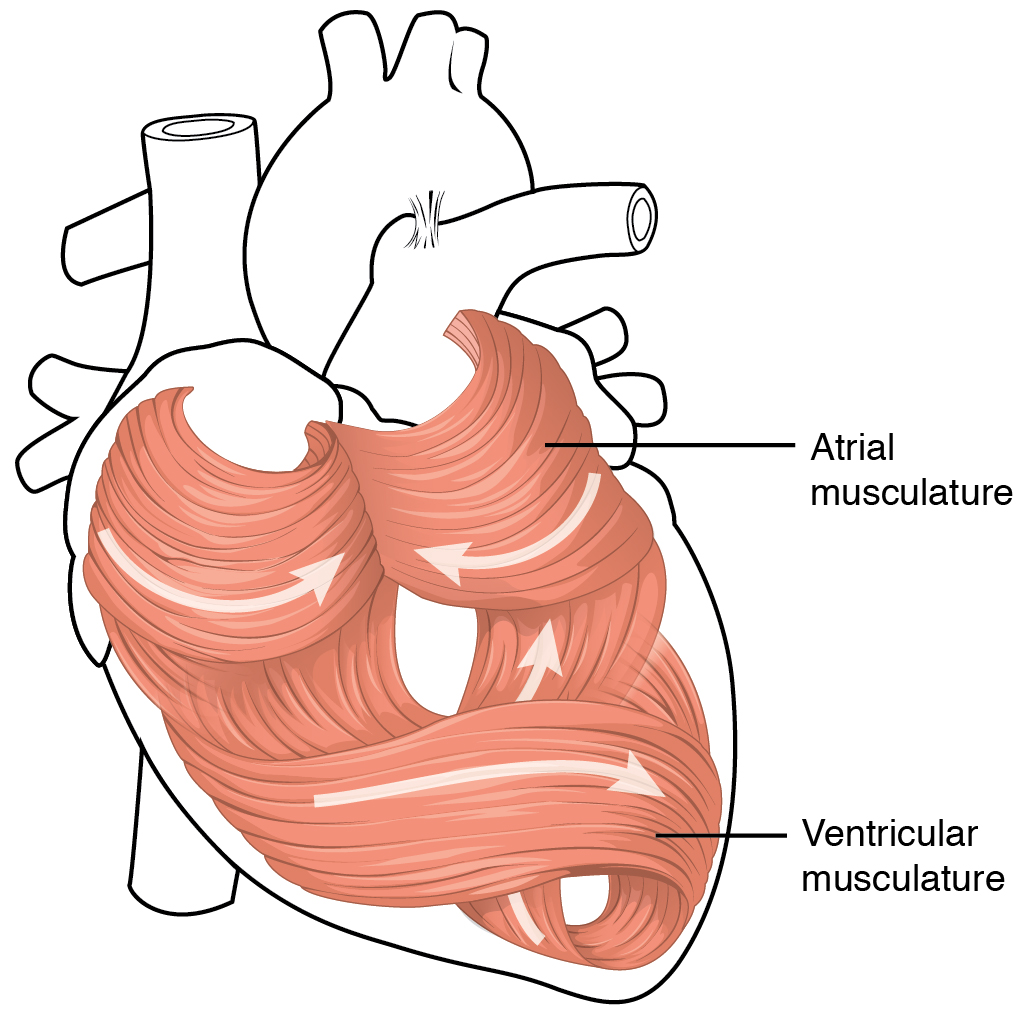
(a) Heart Musculature [51]

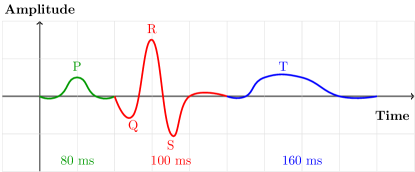
(b) An ecg Waveform Illustration

Figure 1: Illustration of a Heart and an ecg Waveform

II System Model and Task Formulation

In this section, we lay the groundwork for the subsequent derivation of the hkf. We begin with a review of essential information on the ecg signal. Following that, we delve into the task of multi-channel ecg signal denoising. We conclude by presenting our unique hierarchical ss model, which serves as the foundation for the hkf design.

II-A The ECG Signal

The heart is composed of two main types of muscle: the atrial muscle and the ventricular muscle, as illustrated in Figure 1(a). During a hb (hb), these different muscles contract and relax in response to electrical impulses, which depolarize and repolarize the heart. These impulses propagate as an electrical field through the body and can be detected by electrodes on the skin. The voltage variation recorded over time is what we refer to as the ecg signal. The typical ecg signal comprises three segments: the P-wave, the QRS complex, and the T-wave, as shown in Figure 1(b). Each of these segments represents a different stage of heart contraction. The P-wave corresponds to the contraction of the atrial muscle; the QRS complex indicates ventricular depolarization; and the T-wave reflects ventricular repolarization. As its name suggests, the QRS complex consists of three smaller waves (Q-wave, R-wave, and S-wave) associated with the depolarization of the ventricular muscle. The entire QRS complex cycle takes about 100 $\left[\textrm{msec}\right]$ [52]. While a typical ecg signal depicts positive peaks for the P-wave, R-wave, and T-wave, the direction of these peaks can vary depending on the placement of the electrodes. The bandwidth of an ecg signal usually falls within the 0.05-100 $\mathrm{Hz}$ range [53].

II-B Multi-Channel ECG Denoising Task Formulation

The electrical activity of the heart is observed and monitored by placing multiple electrodes on the human body and recording the noisy amplitudes as a vector time series. Here, each electrode is referred to as a channel. The vector $\mathbf{y}_{t}\in\mathbb{R}^{m}$ denotes the observed noisy amplitudes across $m$ channels in a discrete-time index $t\in\mathbb{Z}$. The specific features of this recording, such as ecg shape, amplitude, noise, and other artifacts, depend on the electrode and its placement on the body. We assume that $\mathbf{y}_{t}$, the noisy recordings, originated from $\mathbf{x}_{t}\in\mathbb{R}^{m}$, multi-channel noiseless signals, that were then corrupted by agn $\mathbf{v}_{t}$. The ecg denoising task is hereby defined as the reconstruction of $\mathbf{x}_{t}$, the $m$ clean channels, from $\left\{\mathbf{y}_{i}\right\}_{i=1}^{t}$, their corresponding past and current noisy observations, namely

$$\Psi:\left\{\mathbf{y}_{i}\right\}_{i=1}^{t}\mapsto\hat{\mathbf{x}}_{t},\hskip 7.82433pt\Psi^{\ast}=\arg\min\mathbb{E}{\left\|\hat{\mathbf{x}}_{t}-\mathbf{x}_{t}\right\|^{2}}.$$ (1)

The denoiser, formulated as a mapping $\Psi$, is designed to minimize a cost function. A natural choice for this function is the mse.

The underlying ground truth heart activity is commonly described as a cardiac vector, a stochastic process in $\mathbb{R}^{3}$, that captures the direction and magnitude of the electrical impulses as they propagate through the heart. Therefore we assume that $\mathbf{x}_{t}$, describing the $m$ channels, is intra-correlated, and originates from the same hidden gt activity signal This assumption will be used in our hierarchical system model as shown next.

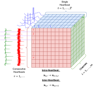
Figure 2: Hierarchical System Model as a Tensor

II-C Hierarchical System Model

The relationship between the observed ecg signal $\mathbf{y}_{t}$ to its corresponding noiseless instance $\mathbf{x}_{t}$, can be modeled as a dynamical system. A canonical way to model dynamical systems in dt is by using ss models [54]. ss models blend well with numerous filtering and smoothing techniques, and can accommodate the integration of both physical and dd learned models. To exploit the periodicity, which plays a key role in the ecg signal, we model the signal dynamics using a hierarchical ss model.

In the following, we make a reasonable assumption that individual hb can be accurately segmented. Therefore, we divide the signal into periodic segments of length $\mathrm{T}$, where each such segment represents a single hb. Our model draws inspiration from the decimated components decomposition method, which is used to represent periodic systems and cyclostationary signals [55] as multivariate (tensor) stationary ones. The dynamics within a single hb are described using an intra-hb (internal) ss model, while the dynamics between two consecutive hb are modeled using an inter-hb (external) ss model, as detailed next.

II-D Intra Heartbeat Modeling

The intra-hb ss model defines the dynamics within a single hb with index $\tau$. For each time step $t$ within the period $\mathcal{T}\triangleq\left\{1,..,\mathrm{T}\right\}$ of length $\mathrm{T}$, the model is given by:

$$\mathbf{x}_{\tau,t} =\mathbf{f}_{t}\left(\mathbf{x}_{\tau,t-1}\right)+\mathbf{e}_{\tau,t}, \mathbf{e}_{\tau,t} \sim\mathcal{N}\left(0,\mathbf{Q}_{t}\right),$$ (2a)

$$\mathbf{y}_{\tau,t} =\mathbf{x}_{\tau,t}+\mathbf{v}_{\tau,t}, \mathbf{v}_{\tau,t} \sim\mathcal{N}\left(0,\mathbf{R}_{t}\right).$$ (2b)

The matrices $\mathbf{Q}_{t}$ and $\mathbf{R}_{t}$ represent the time-varying intra-evolution (process) and observation covariance of a Gaussian distribution, respectively. They capture the correlation across multiple channels. Specifically, $\mathbf{Q}_{t}$ accounts for the correlation arising from the fact that these channels originate from the same foundational heart activity. In contrast, $\mathbf{R}_{t}$ captures the correlation attributed to shared measuring effects: patient-related factors such as breathing and movement, measuring-device-related factors such as quality and age, and environmental factors, including electromagnetic interference and ambient room temperature. As a result, these matrices are assumed to be unknown and are not restricted to be diagonal.

We denote the $\tau$-th hb and its noisy observation as the matrices $\mathcal{X}_{\tau}$ and $\mathcal{Y}_{\tau}$, respectively, namely,

$$\mathcal{X}_{\tau} =\left[\mathbf{x}_{\tau,1},\ldots,\mathbf{x}_{\tau,\mathrm{T}}\right]\in\mathbb{R}^{m\times\mathrm{T}},$$ (3a)

$${\mathcal{Y}_{\tau}} =\left[\mathbf{y}_{\tau,1},\ldots,\mathbf{y}_{\tau,\mathrm{T}}\right]\in\mathbb{R}^{m\times\mathrm{T}}.$$ (3b)

II-E Inter Heartbeat Modeling

The inter-hb ss model defines the evolution between two consecutive hb, labeled with indices $\tau-1$ and $\tau$, namely:

$$\mathbf{x}_{\tau,t} =\mathcal{F}\left(\mathbf{x}_{\tau-1,t}\right)+\boldsymbol{\epsilon}_{\tau,t}, \boldsymbol{\epsilon}_{\tau,t} \sim\mathcal{N}\left(0,\mathcal{Q}_{\tau,t}\right),$$ (4a)

$$\tilde{\mathbf{y}}_{\tau,t} =\mathbf{x}_{\tau,t}+{\boldsymbol{\nu}}_{\tau,t}, {\boldsymbol{\nu}}_{\tau,t} \sim\mathcal{N}\left(0,\mathcal{R}_{\tau,t}\right).$$ (4b)

Based on the periodicity of the cardiac vector, here, we assume that two consecutive hb closely resemble each other, therefore, the inter-state evolution is defined as the identity mapping, i.e., $\mathcal{F}\left(\mathbf{x}\right)=\mathbf{x}$. The matrices $\mathcal{Q}_{\tau,t}$ and $\mathcal{R}_{\tau,t}$ represent the inter-evolution (process) and observation covariance respectively. These matrices capture the multi-channel correlation, and they adhere to the same assumptions outlined for the inter-HB model.

$$\mathbf{Y}_{\tau}=\left[\tilde{\mathbf{y}}_{\tau,1},\ldots,\tilde{\mathbf{y}}_{\tau,\mathrm{T}}\right]\in\mathbb{R}^{m\times\mathrm{T}}.$$ (5)

An illustrative overview of the system model can be found in Figure 2.

III HKF - Hierarchical Kalman Filter

Our custom-designed hkf exploits the proposed hierarchical ss model to perform patient-dependent denoising.

III-A Overview and Design Rationale

There are two main phases to the algorithm:

1. A short online warm-up phase.

2. A signal-denoising processing phase.

In P1, the online warm-up phase, we learn the internal parameters of the intra-hb ss model (2), specifically: the prior signal evolution model and the noise covariance matrices. The specific hb shape varies considerably among patients and can be influenced by numerous factors, ranging from physiological to equipment-related and ambient factors. Consequently, pre-training an algorithm on a ds from multiple patients results in learning an average heartbeat waveform. To avoid this, our algorithm is designed to adapt to individual patients, learning the signal model in an unsupervised manner. In particular, we employ Taylor ls, detailed in Subsection IV-A, for the evolution function approximation. Meanwhile, the unknown noise covariance matrices are estimated using a variant of the em algorithm, as elaborated upon in Subsection IV-C.

Next, in phase P2, the signal-denoising processing phase, each new hb $\mathcal{X}_{\tau}$ is denoised by fusing $\mathcal{Y}_{\tau}$, its noisy observation, with $\left\{\mathcal{Y}_{\tau^{\prime}}\right\}_{\tau^{\prime}=1}^{\tau-1}$, which encapsulates all previous information. Namely:

$$\Psi:\left\{\mathcal{Y}_{\tau^{\prime}}\right\}_{\tau^{\prime}=1}^{\tau}\mapsto\hat{\mathcal{X}}_{\tau}$$ (6)

The fusion process is conducted efficiently through a recursive update, which fuses the new observation with the previous posterior, $\hat{\mathcal{X}}_{\tau}$, acting as a sufficient statistic for the accumulated information. This approach is underpinned by the SS models outlined earlier. Namely:

$$\Psi:\hat{\mathcal{X}}_{\tau-1},\mathcal{Y}_{\tau}\mapsto\hat{\mathcal{X}}_{\tau}$$ (7)

Here, for enhanced clarity, we use $\hat{\mathcal{X}}_{\tau}$ to denote $\hat{\mathcal{X}}_{\tau\left|\tau\right.}$, which represents the mean of the posterior distribution, given $\tau$ hb.

In practice, the denoising is implemented in two steps as in the following:

1. Intra-hb Kalman smoothing.

2. Inter-hb Kalman filtering.

In D1, the rts smoother [50, 48] is used to compute $\tilde{\mathcal{X}}_{\tau}$, an intermediate denoised version, from $\mathcal{Y}_{\tau}$, in a stand-alone manner, based on the intra-hb ss model (2), given the learned prior parameters. More specifically:

$$\tilde{\Psi}:\mathcal{Y}_{\tau}\mapsto\tilde{\mathcal{X}}_{\tau}=\left[\hat{\mathbf{x}}_{\tau,1\left|\mathrm{T}\right.},\ldots,\hat{\mathbf{x}}_{\tau,\mathrm{T}\left|\mathrm{T}\right.}\right]\in\mathbb{R}^{m\times\mathrm{T}}.$$ (8)

Here, the notation $\hat{\mathbf{x}}_{\tau,t\left|\mathrm{T}\right.}$ denotes the smoothed version of sample $t$ in hb $\tau$ given all $\mathrm{T}$ samples from the entire hb. This stage is detailed in Subsection III-B.

In D2, the kf is used to compute $\hat{\mathcal{X}}_{\tau}$, the fully denoised posterior hb, by fusing $\mathbf{Y}_{\tau}=\tilde{\mathcal{X}}_{\tau}$, i.e., the stand-alone smoothed version, with $\hat{\mathcal{X}}_{\tau-1}$, the fully denoised posterior of the previous heartbeat. This stage is based on the inter-hb ss model (4), with an adaptive covariance estimation. More specifically:

$$\hat{\Psi}:\hat{\mathcal{X}}_{\tau-1},\tilde{\mathcal{X}}_{\tau}\!\mapsto\!\hat{\mathcal{X}}_{\tau}\!=\!\left[\hat{\mathbf{x}}_{\tau\left|\tau\right.,1\left|\mathrm{T}\right.},\ldots,\hat{\mathbf{x}}_{\tau\left|\tau\right.,\mathrm{T}\left|\mathrm{T}\right.}\right].$$ (9)

This operation represents a batch of $\mathrm{T}$ parallel kf. In this context, the additional notation $\tau\left|\tau\right.$ denotes the update of the smoothed version, incorporating information from the current and all previous hb. Further details are provided in  Subsection III-C.

Figure 3 visualizes the high-level structure of the processing phase, while Figure 4 is a high level description of our hkf algorithm.

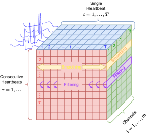
Figure 3: Processing Phase - Smoothing and Filtering

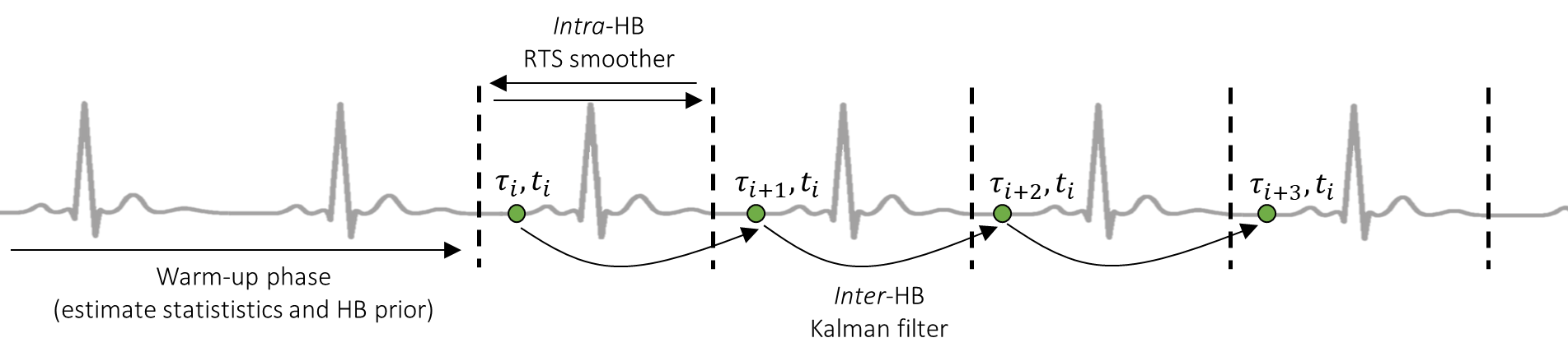
Figure 4: HKF Overview

III-B First Stage Smoothing

In the processing phase, the first step, D1, involves implementing a ks using the rts algorithm [50]. This ks operates based on the intra-hb ss model parameters (2): $\hat{\mathbf{f}}_{t}$, $\hat{\mathbf{Q}}_{t}$, and $\hat{\mathbf{R}}_{t}$, learned during the warm-up phase. Given $\mathcal{Y}_{\tau}$, the newly observed hb with index $\tau$, we employ the ks, denoted as $\tilde{\Psi}$, to obtain an instantaneous estimate of the denoised hb, denoted as $\hat{\mathcal{X}}_{\tau}$.

The rts smoother encompasses two-steps:

1. A forward pass step, i.e., a kf.

2. A backward pass step.

The forward pass, KS1, is defined by two phases: prediction and update The prediction phase, is given by state prediction:

$$\hat{\mathbf{x}}_{t\left|t-1\right.}=\mathbf{f}_{t}\left(\hat{\mathbf{x}}_{t-1\left|t-1\right.}\right),\quad\mathbf{P}_{t\left|t-1\right.}=\mathbf{P}_{t-1\left|t-1\right.}+\mathbf{Q}_{t},$$ (10)

where $\mathbf{P}_{t\left|t-1\right.}$, the prior covariance, is computed using an identity matrix, as defined in (29), and by innovation prediction:

$$\hat{\mathbf{y}}_{t\left|t-1\right.}=\hat{\mathbf{x}}_{t\left|t-1\right.},\quad\Delta\mathbf{y}_{t}=\mathbf{y}_{t}\!-\!\hat{\mathbf{y}}_{t\left|t-1\right.},\quad\mathbf{S}_{t}=\mathbf{P}_{t\left|t-1\right.}+\mathbf{R}_{t}.$$ (11)

The update phase is given by:

$$\hat{\mathbf{x}}_{t\left|t\right.}=\hat{\mathbf{x}}_{t\left|t-1\right.}\!+\!\mathcal{K}_{t}\cdot\Delta\mathbf{y}_{t},\quad\mathbf{P}_{t\left|t-1\right.}-\mathcal{K}_{t}\cdot\mathbf{S}_{t}\cdot\mathcal{K}_{t}^{\top}.$$ (12)

Here, $\mathcal{K}_{t}$ is the kg, given by:

$$\mathcal{K}_{t}=\mathbf{P}_{t\left|t-1\right.}\cdot\mathbf{S}_{t}^{-1}$$ (13)

The backward pass, KS2, of the rts smoother is given by:

$$\hat{\mathbf{x}}_{t\left|\mathrm{T}\right.}=\hat{\mathbf{x}}_{t\left|t\right.}+\mathcal{G}_{t}\cdot\Delta\mathbf{x}_{t},\quad\mathbf{P}_{t\left|\mathrm{T}\right.}=\mathbf{P}_{t|t}-\mathcal{G}_{t}\cdot\Delta\mathbf{P}_{t+1}\cdot\mathcal{G}_{t}.$$ (14)

$$\Delta\mathbf{x}_{t}=\hat{\mathbf{x}}_{t+1\left|\mathrm{T}\right.}-\hat{\mathbf{x}}_{t+1\left|t\right.},\quad\Delta\mathbf{P}_{t+1}=\mathbf{P}_{t+1\left|\mathrm{T}\right.}-\mathbf{P}_{t+1\left|t\right.}$$ (15)

Here, $\mathcal{G}_{t}$, the smoothing gain, is given by:

$$\mathcal{G}_{t}=\mathbf{P}_{t\left|t\right.}\mathbf{P}_{t+1\left|t\right.}^{-1}.$$ (16)

The output of the smoothing step is

$$\tilde{\mathcal{X}}_{\tau}=\tilde{\Psi}\left(\mathcal{Y}_{\tau}\right)=\left[\hat{\mathbf{x}}_{\tau,1\left|\mathrm{T}\right.},\ldots,\hat{\mathbf{x}}_{\tau,\mathrm{T}\left|\mathrm{T}\right.}\right].$$ (17)

We assume that the estimated distribution for the instantaneously denoised hb is given by

$$\mathbf{x}_{\tau,t\left|\mathrm{T}\right.}\sim\mathcal{N}\left(\hat{\mathbf{x}}_{\tau,t\left|\mathrm{T}\right.},\mathbf{P}_{\tau,t\left|\mathrm{T}\right.}\right)$$ (18)

This distribution is significant for the subsequent filtering stage detailed in Subsection III-C. We will use $\hat{\mathbf{x}}_{t\left|\mathrm{T}\right.}$, the posterior mean, and $\mathbf{P}_{\tau,t\left|\mathrm{T}\right.}$, the posterior error covariance estimate, from the initial stage as observations and observation noise for the second stage, respectively. This approach not only eliminates the need for an additional estimation step but also offers the optimal estimate of the observation noise matrices, under the assumption that all previously estimated values are optimal.

III-C Second Stage Filtering

In the second step, D2, of the processing phase, we employ a kf based on the inter-hb ss model (4). Given the immediate estimate of the current hb, denoted as $\tilde{\mathcal{X}}_{\tau}$, and the posterior estimate of the preceding hb accounting for its entire past $\hat{\mathcal{X}}_{\tau-1}$, we produce a posterior estimate for the current hb $\hat{\mathcal{X}}_{\tau}$. This filter effectively unfolds to $\mathrm{T}$ kf operating simultaneously along the $\tau$-axis:

$$\Psi^{*}_{t}:\hat{\mathbf{x}}_{\tau,t\left|\mathrm{T}\right.},\hat{\mathbf{x}}_{\tau-1\left|\tau-1\right.,t\left|\mathrm{T}\right.}\mapsto\hat{\mathbf{x}}_{\tau\left|\tau\right.,t\left|\mathrm{T}\right.}.$$ (19)

In the end, we leverage the temporal correlation between two successive hb, $\tau-1$ and $\tau$, as outlined in (4). For every $t\in\mathcal{T}$ and given the estimated covariance matrices, we implement $\mathrm{T}$ independent (and parallel) kf. This procedure is articulated in the ensuing steps; note that for simplicity, we occasionally omit the intra-hb index $t$.

1. Prior error and innovation covariance:

   $$\mathcal{P}_{\tau\left|\tau-1\right.}=\mathcal{P}_{\tau-1}+\hat{\mathcal{Q}}_{\tau},\quad\mathcal{S}_{\tau}=\mathcal{P}_{\tau\left|\tau-1\right.}+\hat{\mathcal{R}}_{\tau}.$$ (20)

2. The update equations:

   $$\hat{\mathcal{X}}_{\tau}=\hat{\mathcal{X}}_{\tau-1}+\mathbfcal{K}_{\tau}\cdot\Delta,\quad\mathcal{P}_{\tau}=\mathcal{P}_{\tau\left|\tau-1\right.}-\mathbfcal{K}_{\tau}\cdot{\mathcal{S}_{\tau}}\cdot\mathbfcal{K}^{\top}_{\tau}.$$ (21)

Here, $\Delta$ is the innovation, and $\mathbfcal{K}_{\tau}$ is the Kalman gain:

$$\Delta=\tilde{\mathcal{X}}_{\tau}-\hat{\mathcal{X}}_{\tau-1}=\left(\hat{\mathbf{x}}_{\tau,t\left|\mathrm{T}\right.}-\hat{\mathbf{x}}_{\tau-1\left|\tau-1\right.,t\left|\mathrm{T}\right.}\right)_{\forall t},$$ (22)

$$\mathbfcal{K}_{\tau}=\mathcal{P}_{\tau\left|\tau-1\right.}\cdot\mathcal{S}_{\tau}^{-1}$$ (23)

To successfully deploy the kf the set of inter-hb covariance matrices, i.e.,

$$\left\{\mathcal{Q}_{\tau,t},\mathcal{R}_{\tau,t}\right\}_{t=1}^{\mathrm{T}}$$ (24)

should be estimated on the fly before the filtering step. The estimation of the observation noise is provided in Subsection IV-D, while the estimation of the process noise is provided in Subsection IV-E.

III-D Signal Pre-Processing

The accurate detection of the various peaks and intervals within an ecg waveform, such as R-peaks and QT-interval, often provides vital clinical information. Over the years, a multitude of methods have been developed to address this complex task. Classical approaches typically utilize the time-derivatives of the recorded signal, applying thresholding on parameters such as slew-rate [56] or directly to the derivative [57]. Some methods attempt to fit local ss models to a given signal, then detecting peaks by observing sudden changes in the model using a log-cost ratio [58].

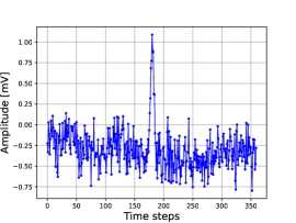
Figure 5: Example of noisy observation $\mathcal{Y}_{\tau}$ after pre-processing.

Our HKF algorithm operates under the assumption that each hb, represented as $\mathcal{X}_{\tau}$, can be isolated during a pre-processing phase and subsequently processed independently. The central idea hinges on detecting R-peaks and processing a set of samples centered around them. The width of this processing window is proportional to the sampling frequency of the utilized ECG recording device (e.g. $f_{s}=360$\mathrm{Hz}$\rightarrow$ translates to 360 data points per hb). A vast array of off-the-shelf peak-detection algorithms exist, ranging from wavelet transform-based methods like [59, 60], to nn (nn) based techniques such as [61]. For our empirical studies, we leveraged the python bioSPPy library [62], which is based on [63, 64]. An example of a pre-processed observation is illustrated in Figure 5.

III-E Signal Post-Processing

After successfully filtering an individual HB, it can be seamlessly integrated with previously filtered HBs to form a continuous signal. Given the fixed window length $T$ applied during pre-processing, there are two potential scenarios that can arise based on the hr (hr): Overlaps (denoted as PP1) and Gaps (denoted as PP2).

1. Overlaps: In this scenario, a weighted average of the reconstructed version can be employed as the estimated continuous signal.

2. Gaps: For gaps between heartbeats, linear interpolation is chosen to bridge the gap between the end of the hb with index $\tau$ and the beginning of the subsequent hb with index $\tau+1$. This approach is justified as there’s typically no significant heart activity between these two periods, and the region usually consists predominantly of white noise.

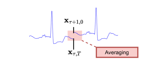
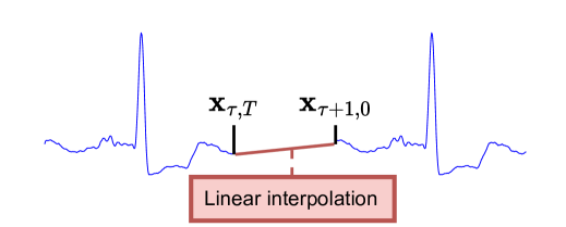
Figure 6: Reconstruction of Continuous ecg

A visual representation of these two methodologies can be referenced in Figure 6.

IV Online Prior Learning and Parameter Estimation

In this section, we delve into the process of parameter learning. Specifically, we discuss how to determine the parameters for the intra-hb Kalman smoothing (D1) during the online warm-up phase (P1). We will also cover the learning of parameters for the inter-hb Kalman filtering (D2).

IV-A Online Learned Taylor Priors

The primary objective of the online warm-up phase (P1) is to determine a patient-specific characterization of the intra-hb ss model (2) parameters, with a particular focus on the ecg waveform signal evolution model. Given the complexities of the ecg signal, identifying a closed-form function that can accurately depict its evolution is challenging. As a solution, we adopt a Taylor function approximation as our point-wise evolution model. The Taylor model provides insight into how a function behaves near a specific point, making it suitable for this purpose. Owing to the periodic nature of the ecg signal, characterizing such a prior for one period, $\tau$, ensures its applicability across all periods.

$$\mathbf{x}_{\tau,t}=\mathbf{f}_{t}\left(\mathbf{x}_{\tau,t-1}\right)=\mathbf{x}_{\tau,t-1}+\Delta\mathbf{x}_{\tau,t},\quad t\in\mathcal{T}$$ (25)

In this context, $\mathbf{x}$ is a function of $t$. Hence, for a sufficiently small time discretization interval, $\Delta t$, we can approximate $\Delta\mathbf{x}_{\tau,t}$ using a finite Taylor expansion, provided that $K$ is sufficiently large.

$$\Delta\mathbf{x}_{\tau,t}=\mathbf{x}_{\tau,t}-\mathbf{x}_{\tau,t-1}\simeq\sum_{k=1}^{K}\frac{d^{k}}{dt^{k}}\mathbf{x}_{\tau,t-1}\cdot\frac{\Delta t^{k}}{k!}=\mathbf{F}_{t}\cdot\phi\left(\Delta t\right).$$ (26)

Here, $\phi\in\mathbb{R}^{K\times 1}$ is a vector of a basis functions, namely:

$$\phi^{\top}\left(\Delta t\right)=\begin{pmatrix}\frac{\Delta t^{1}}{1!},\cdots,\frac{\Delta t^{K}}{K!}\end{pmatrix},$$ (27)

and $\mathbf{F}_{t}\in\mathbb{R}^{m\times K}$ is designated as a matrix of coefficients, formulated as:

$$\mathbf{F}_{t}=\begin{pmatrix}\frac{d^{1}}{dt^{1}}\mathbf{x}_{t-1,\tau},\cdots,\frac{d^{K}}{dt^{K}}\mathbf{x}_{t-1,\tau}\end{pmatrix}.$$ (28)

Considering this, the Jacobian matrix, $\mathcal{J}_{\mathbf{f}}$, which is necessary for integrating the evolution into an ekf (ekf), simplifies to an identity matrix. Specifically:

$$\mathcal{J}_{\mathbf{f}}=\frac{\mathrm{d}\mathbf{x}_{\tau,t}}{\mathrm{d}\mathbf{x}_{\tau,t-1}}=\frac{\mathrm{d}\mathbf{f}_{t}\left(\mathbf{x}_{\tau,t-1}\right)}{\mathrm{d}\mathbf{x}_{\tau,t-1}}=\mathbf{I}_{m\times m}$$ (29)

This comes in handy in equation (10).

IV-B Learning a Taylor Approximation

The matrix $\mathbf{F}_{t}$, which remains to be determined, can be learned in an unsupervised manner from a set of noisy observations of size $N$. This set is given by:

$$\left\{\Delta\mathbf{y}_{\tau_{i},t}=\mathbf{y}_{\tau_{i},t}-\mathbf{y}_{\tau_{i},t-1}\right\}_{i=1}^{N},$$ (30)

The objective is to minimize a specific ls loss function, specified as:

$$\mathcal{L}\left(\mathbf{F}_{t}\right)=\frac{1}{N}\cdot\sum_{i=1}^{N}\left\|\Delta\mathbf{y}_{\tau_{i},t}-\mathbf{F}_{t}\cdot\phi\right\|^{2},$$ (31)

where $\hat{\mathbf{F}}_{t}$ represents the minimized value:

$$\hat{\mathbf{F}}_{t}=\arg\min\left\{\mathcal{L}\left(\mathbf{F}_{t}\right)\right\}\quad\mathbf{F}_{t}\in\mathbb{R}^{m\times K}.$$ (32)

This optimization problem offers a clear, closed-form solution. It can be efficiently computed through a single multiplication of an online-generated column vector $\Delta\overline{\mathbf{y}}_{t}$ by a constant row vector $\mathbf{g}$, namely:

$$\hat{\mathbf{F}}_{t}=\Delta\overline{\mathbf{y}}_{t}\cdot\mathbf{g},$$ (33)

where

$$\Delta\overline{\mathbf{y}}_{t}=\frac{1}{N}\cdot\sum_{i=1}^{N}\Delta\mathbf{y}_{\tau_{i},t},\quad\mathbf{g}=\phi^{\top}\cdot\left(\phi\cdot\phi^{\top}\right)^{-1}.$$ (34)

The effectiveness and reliability of our estimator are influenced by the number of observations used for its computation. This, in turn, relies on the number of hb utilized to gather data. An additional objective is to ensure the smooth evolution of our ecg waveform. To achieve this smoothness, we can aggregate multiple observations in the close proximity of ts of ts and adapt our loss function accordingly:

$$\mathcal{L}_{\alpha}\left(\mathbf{F}_{t}\right)=\frac{1}{N}\cdot\sum_{i=1}^{N}\sum_{j=-M}^{M}\alpha_{j}\cdot\left\|\Delta\mathbf{y}_{\tau_{i},t+j}-\mathbf{F}_{t}\cdot\phi\right\|^{2}.$$ (35)

Specifically, we employ a window spanning $2M+1$ with decaying weights $\alpha_{j}$ that sums up to one:

$$\sum_{j=-M}^{M}\alpha_{j}=1.$$ (36)

The weighted ls optimization problem in (35) also admits a straightforward solution, given by:

$$\hat{\mathbf{F}}_{\alpha,t}=\Delta\overline{\overline{\mathbf{y}}}_{t}\cdot\mathbf{g},\quad\Delta\overline{\overline{\mathbf{y}}}_{t}=\frac{1}{N}\cdot\sum_{i=1}^{N}\sum_{j=-M}^{M}\alpha_{j}\cdot\Delta\mathbf{y}_{\tau_{i},t+j}.$$ (37)

IV-C Online Covariance Learning

In the second stage of our proposed warm-up phase P1, the primary objective is to estimate the missing covariance matrices for the intra-hb ss model (2). Specifically, we aim to determine the intra-evolution covariance, $\mathbf{Q}_{t}$, and the intra-observation covariance, $\mathbf{R}_{t}$. To achieve this, we employ the em algorithm. The em algorithm, an iterative method, has been frequently adapted for the task of parameter estimation in ss models [65, 66, 67].

The em algorithm operates by alternating between the E-step and the M-step. During the E-step, we compute the conditional expectation. For our application, this involves calculating the posterior moments using the rts smoother for each ts $t\in\mathcal{T}$. Specifically, from the rts smoother, we derive the first-order moment $\hat{\mathbf{x}}_{t\left|\mathrm{T}\right.}$, the covariance matrix $\mathbf{P}_{t\left|\mathrm{T}\right.}$, and the backward smoothing gain $\mathcal{G}_{t}^{\top}$. With these values, we can then determine the posterior second-order moments, namely:

$$\mathbf{X}^{\mathrm{II}}_{t}=\hat{\mathbf{x}}_{t\left|\mathrm{T}\right.}\cdot\hat{\mathbf{x}}_{t\left|\mathrm{T}\right.}^{\top}+\mathbf{P}_{t\left|\mathrm{T}\right.},\quad\mathbf{Y}^{\mathrm{II}}_{t}=\mathbf{y}_{t}\cdot\mathbf{y}_{t}^{\top},$$ (38)

and the posterior correlations:

$$\mathbf{XY}_{t,t} =\hat{\mathbf{x}}_{t\left|\mathrm{T}\right.}\cdot\mathbf{y}_{t}^{\top},$$ (39a)

$$\mathbf{XX}_{t,t-1} =\hat{\mathbf{x}}_{t\left|\mathrm{T}\right.}\cdot\hat{\mathbf{x}}_{t-1\left|\mathrm{T}\right.}^{\top}+\mathbf{P}_{t\left|\mathrm{T}\right.}\cdot\mathcal{G}_{t-1}^{\top}.$$ (39b)

In the M-step, we employ mle, drawing upon the results of the previous step, to derive an instantaneous estimate for the unknown covariance matrices, as outlined next:

$$\tilde{\mathbf{Q}}_{t} =\mathbf{X}^{\mathrm{II}}_{t}-2\cdot\mathbf{XX}_{t,t-1}+\mathbf{X}^{\mathrm{II}}_{t-1},$$ (40a)

$$\tilde{\mathbf{R}}_{t} =\mathbf{Y}^{\mathrm{II}}_{t}-2\cdot\mathbf{YX}_{t,t}+\mathbf{X}^{\mathrm{II}}_{t}.$$ (40b)

Given the distinct shape of the hb, we operate under the assumption that the observation noise statistic remains invariant within a single hb; that is, it stays consistent over the timescale of a hb. Consequently, by averaging the instantaneous estimators across the entire hb, we obtain a single estimate that holds valid for all ts, as illustrated next:

$$\hat{\mathbf{R}}_{t}=\hat{\mathbf{R}}=\frac{1}{\mathrm{T}}\cdot\sum_{t=1}^{\mathrm{T}}\tilde{\mathbf{R}}_{t}.$$ (41)

While our previous assumption applies to the observation noise statistic, it does not hold true for the process noise statistic. We assume that this statistic is not invariant within a single hb and exhibits temporal correlations over brief periods. Consequently, we take an average of the instantaneous estimators within a short time window of length $\tilde{L}=L_{1}+L_{2}+1$, obtaining:

$$\hat{\mathbf{Q}}_{t}=\frac{1}{L_{1}+L_{2}+1}\cdot\sum_{\ell=-L_{1}}^{L_{2}}\tilde{\mathbf{Q}}_{t+\ell}.$$ (42)

To get a more robust and accurate estimate, we can exploit inter-hb correlations and unfold the em algorithm over multiple hb. Given a sequence of hb, the most straightforward way is to apply the em algorithm on each hb independently, and then average the single hb based estimators to a multi-hb based estimator. The second alternative, which is more aligned with online learning, is to run a single em iteration on the data from hb with index $\tau$, and then plug-in the results into hb with index $\tau+1$ and perform another em iteration. This process should continue until some convergence criteria are met, namely the change in the estimated parameters is small enough. In addition to the fact that the second alternative has lower computational complexity, it often yields much more stable results, as we observe in the empirical study (Section V).

IV-D Inter Heartbeat Observation Noise Estimation

To estimate $\mathcal{R}_{\tau,t}$, the inter-hb observation noise covariance, we observe that $\mathbf{P}_{\tau,t\left|T\right.}$, is the error covariance of the first stage estimation, namely

$$\hat{\mathbf{x}}_{\tau,t\left|\mathrm{T}\right.}-\mathbf{x}_{\tau,t}\sim\mathcal{N}\left(0,\mathbf{P}_{\tau,t\left|T\right.}\right).$$ (43)

Since $\tilde{\mathbf{y}}_{\tau,t}=\hat{\mathbf{x}}_{\tau,t\left|\mathrm{T}\right.}$, the input for the second stage filtering is equal to the output of the first stage smoothing, then we can set $\mathbf{P}_{\tau,t\left|T\right.}$ as $\tilde{\mathcal{R}}_{\tau,t}$, an instantaneous estimate for the second-stage observation noise covariance.

To further smooth our estimate and to improve algorithm’s stability, we exploit inter-hb correlations by averaging the instantaneous estimates in a window of size $L=L_{1}+L_{2}+1$, and get

$$\hat{\mathcal{R}}_{\tau,t}=\frac{1}{L_{1}+L_{2}+1}\sum_{\ell=-L_{1}}^{L_{2}}\tilde{\mathcal{R}}_{\tau,t+\ell}.$$ (44)

IV-E Inter Heartbeat Process Noise Estimation - Single Channel

To estimate the process covariance $\mathcal{Q}_{\tau}$, we employ a mle approach similar to that described in [68]. By examining the ss model equation (4) and the kf equation (20), we establish that, for every $\forall t$, there exists a relationship between the innovation covariance $\mathcal{S}_{\tau}$ and the process covariance $\mathcal{Q}_{\tau}$. An empirical estimate for $\mathcal{S}_{\tau}$ is given by $\Delta\cdot\Delta^{\top}$, with $\Delta$ defined in (22). In estimating the process covariance matrix, it is imperative to ensure the matrix is psd (psd). Consequently, we omit the correlation between different channels during the inter-filtering process and presume a diagonal structure for the covariance matrix. Namely:

$$\tilde{\mathcal{Q}}_{\tau,t}=\tilde{\mathbf{q}}^{2}_{\tau,t}\otimes\mathbf{I}_{m\times m},$$ (45)

where all diagonal entries are positive

$$\tilde{\mathbf{q}}^{2}_{\tau}\left(i\right)=\max\left\{\bar{\mathcal{Q}}_{\tau}\left(i,i\right),0\right\}.$$ (46)

Here,

$$\bar{\mathcal{Q}}_{\tau}=\Delta\cdot\Delta^{\top}-\hat{\mathcal{R}}_{\tau}-\mathcal{P}_{\tau-1}$$ (47)

To get a smoother and more robust estimator we can exploit both intra-hb and inter-hb correlations. We first average our estimator in a local time window

$$\mathcal{Q}_{\tau,t}^{*}=\frac{1}{L_{1}+L_{2}+1}\cdot\sum_{\ell=-L_{1}}^{L_{2}}\tilde{\mathcal{Q}}_{\tau,t+\ell}$$ (48)

and then apply an exponential smoothing, i.e., a simple iir (iir) filter, namely

$$\hat{\mathcal{Q}}_{\tau}=\alpha\cdot\mathcal{Q}_{\tau}^{*}+\left(1-\alpha\right)\cdot\hat{\mathcal{Q}}_{\tau-1}$$ (49)

Where $0<\alpha<1$ is the forgetting factor.

While this option is simpler to compute, it is not always optimal as can be seen in the empirical results in Section V. Next, we relive that assumption, to exploit inter-channel correlation.

IV-F Inter Heartbeat Process Noise Estimation - Multi Channel

To enhance our denoising algorithm’s performance, we aim to relax the constraint that mandates the covariance matrix to be diagonal, thereby leveraging intra-heartbeat correlations. A primary requirement in estimating a covariance matrix is its psd. While diagonal matrices with positive real entries are naturally psd, this is not the case for arbitrary covariance matrices. Unlike diagonal matrices, there isn’t a straightforward criterion to ensure a matrix’s psd property without significantly altering the matrix, such as modifying the eigenvalue matrix in a spectral decomposition. Thus, directly maximizing the closed-form solution may lead to filter instabilities. This is because the optimal estimate doesn’t inherently adhere to the psd condition, rendering it unsuitable for accurately defining the covariance of a Gaussian distribution. To address this challenge, especially in the context of our second estimation, it becomes imperative to explicitly enforce the psd constraint. We propose accomplishing this using a variant of the rmgd (rmgd) algorithm [69].

rmgd is an advanced optimization technique that builds on the principles of traditional gradient descent. Its uniqueness lies in its ability to optimize on curved spaces called manifolds, making it especially valuable for matrices like the psd ones of size ${m}\times{m}$. These matrices naturally span a manifold $\mathcal{S}^{+}$ within $\mathbb{R}^{\frac{m\times\left(m+1\right)}{2}}$, visualized as a convex cone with symmetric matrices forming its tangent space, denoted $T_{p}\mathcal{S}^{+}=\mathcal{S}$ [70].

To optimize on $\mathcal{S}^{+}$, a tailored inner product on its tangent space, expressed as:

$$g_{p}:T_{p}\boldsymbol{\cdot}\mathcal{S}^{+}\rightarrow\mathbb{R},$$ (50)

converts it into a Riemannian manifold [71]. This structured geometric space significantly impacts the gradient computations. Among the available metrics [72, 73], we chose the log-Cholesky metric [74] due to its efficient closed-form solution for the exponential map, a crucial component of rmgd.

The core rmgd procedure begins by computing the gradient of our loss based on the current estimate. This gradient is then projected onto the manifold’s tangent space. Using the exponential map, we traverse the negative gradient on $\mathcal{S}^{+}$, ensuring our estimate remains psd.

The detailed mathematical description of this algorithm is out of the scope of this paper and it can be found in our code 

IV-G Discussion

The proposed hkf leverages both intra- and inter-hb relations through the introduced ss model and can process multi-dimensional data. This feature enables the exploitation of spatial relations across ecg signals recorded using multiple electrodes. Although our derivation involves several simplifications—particularly regarding the properties of process and observation noise covariances—these make the hkf analytically tractable and ensure the computational demands remain relatively manageable. We observed improvements when integrating multi-channel information during the inter-filtering process. Furthermore, exploring additional techniques to achieve faster estimates of the covariance matrices could be fruitful.

A natural extension of hkf would involve replacing the intra- and inter-HB smoothing and filtering with the recently proposed RTSNet and KalmanNet [75, 76], respectively. This modification would yield a hybrid mb / dd ecg denoiser. We anticipate that such extensions, reserved for future exploration, will further boost performance by relaxing the aforementioned simplifications and enhancing hkf’s noise tolerance.

Given that hkf is anchored in a statistical Bayesian approach, it is possible to extend it into an algorithm that can filter ecg, regardless of the presence of arrhythmia, and concurrently detect arrhythmias. This detection might employ a likelihood-ratio test contrasting the intra- and inter-filters. There are numerous potential applications for hkf, such as its incorporation into smartwatches or its use in monitoring oxygen levels during labor. Each potential application presents its own set of challenges that warrant exploration. For instance, it would be vital to assess the interplay between the algorithms separating fetal from maternal signals in relation to hkf, or to address the subtleties of lower amplitude signals typical in these scenarios.

V Empirical Study

Next, we empirically evaluate the hkf algorithm’s performance. We begin by comparing hkf with multiple benchmark algorithms, using two different ecg recording ds. Initially, we discuss the performance of our algorithm for patients without arrhythmia, representing our algorithm’s primary use case. We then showcase its efficacy for patients with arrhythmia and detail how the algorithm should be adapted for such scenarios. In the appendix, we provide an analysis illuminating the implications of certain design choices.

For the numerical evaluation, two distinct ecg recording datasets were utilized. The first is the widely recognized MIT-BIH dataset, which is publicly accessible [77], while the second dataset is proprietary. This selection ensures the algorithm’s compatibility across various recording devices, sampling frequencies, and channel configurations.

Given that the datasets contain clean ecg recordings, we artificially introduced ecg to simulate a noisy environment. The mse in relation to the clean signal served as our primary performance metric. However, it’s important to acknowledge that in clinical evaluations, other factors, such as wave shape and clarity, are also significant.

V-A Benchmark Algorithms

For our evaluation, the complete hkf was employed. The intermediary output of the first stage ks operation carries the label (ks-intra), and the final independent hkf output is denoted as (hkf). We’ve also presented the multichannel estimate under the label (hkf rmgd). Furthermore, results from applying only the inter-hb filtering, as highlighted in [40], are labeled as (kf-inter).

In addition to these, we included a filtered estimate generated by a data-driven convolutional ae (ae) following the methodologies in [20, 21], marked as (ae). To ensure optimal ae performance, training encompassed the entire dataset, excluding the tested subject. The full details are provided in our code.

V-B Patients without Arrhythmia - Proprietary Dataset

We next turn our attention to the evaluation of our algorithm on patients without arrhythmia, using a proprietary dataset. This dataset offers clean ecg recordings of adults, captured at a sampling rate of $500$\mathrm{Hz}$$. To emulate fetal ecg signals, two modifications were applied to this data:

1. Given that the fetal hr is typically double that of an adult, the ecg signals were subsampled by a factor of two. This creates signals that appear to have a hr twice as high, with a resultant sampling rate of $250$\mathrm{Hz}$$.

2. An attenuation of the signal amplitude was performed to simulate the often weaker amplitude seen in fetal ecg. This diminished amplitude can be attributed to the smaller size of the fetal heart and the typical recording conditions where the ecg is taken from the mother’s abdomen rather than directly from the fetal thorax.

Our algorithm’s robust performance, especially when compared with alternative methods on ecg signals corrupted to $0\left[\textrm{dB}\right]$ snr, is detailed in Table I. Given that the ecg signal was captured using $m=12$ observation channels, our hkf with rmgd effectively leverages correlations between these multiple channels, consistently outpacing other methods in performance. Visual representations showcasing our algorithm’s efficacy can be viewed in the subsequent figures: 14, 9(a), 14, 9(b), 14, and 9(c).

V-C Patients without Arrhythmia - MIT BIH Dataset

Next, we assess our algorithm using patients without arrhythmia from the MIT-BIH (Arrhythmia) ds. This ds comprises $48$ two-channel ambulatory ecg signals recorded by the BIH Arrhythmia Laboratory between 1975 and 1979. These signals were recorded at a rate of $360$ samples per second with an $11$-bit resolution over a $10\unit{\milli}$ range. This ds is widely recognized in the ecg denoising community and serves as a reliable benchmark for evaluating algorithm performance. Examples of its application can be found in references [26, 32, 22].

The results outlined in Table II, showcase hkf’s strong performance, especially when compared with alternative methods, on ecg signals corrupted to $3\left[\textrm{dB}\right]$ snr. Given that the ecg signal was acquired using $m=2$ observation channels, our hkf, which employs a diagonal process covariance matrix, typically outperforms the rmgd version—though performance may vary depending on the specific patient. Visual representations of our algorithm’s efficacy can be found in Figures: 14, 9(d), 14, and 9(e).

The algorithm demonstrates significant capability in denoising ecg signals. Particularly in cases free of arrhythmia, noticeable snr enhancements are evident. It’s also worth highlighting that the inter-channel filter doesn’t merely force a prior onto a signal. This is apparent in Figure 9(f), where the signal’s shape shifts between the $6$th and $8$th seconds, a change that the hkf successfully captures. This adaptability positions hkf as an excellent tool for monitoring variations in signal shape, potentially useful in contexts like detecting heart attacks or acute hypoxia during labor.

V-D Patients with Arrhythmia

Next, we delve deeper into the ecg recordings of patients from the MIT-BIH ds who exhibit various types of arrhythmia, specifically, patients 102 (Figure 9(f)), 107 (Figure 9(g)), and 108. Arrhythmias manifest in diverse ways, ranging from accelerated heart rates (atrial fibrillation) or reduced rates (bradycardia) to sporadic episodes of unusually rapid heart rates when at rest (supraventricular tachycardia). These irregularities can be precursors to far graver conditions, including strokes [5].

Given the unpredictable nature of arrhythmia in terms of shape, frequency, and amplitude, these recordings serve as an excellent benchmark for examining the upper limits of our filter. The assessment was carried out similarly to previous tests: a clean ecg recording was corrupted by agn to achieve a $3\left[\textrm{dB}\right]$ snr, and the denoised output was compared with the original version.

In situations where arrhythmia is evident, the assumption that sequential heartbeats are identical becomes invalid. Specifically, the inter-state evolution function, $\mathcal{F}\left(\cdot\right)$ from (4), doesn’t remain an identity function. Consequently, from the numerical mse findings presented in table III, it’s evident that the complete hkf is outperformed by its intermediary intra-hb smoother output, denoted as ks-intra. This result is logical, given that we cannot enhance performance by merging consecutive hb. Therefore, for patients with arrhythmia, our recommendation is to solely deploy the first stage of smoothing, bypassing the subsequent stage of filtering. In such scenarios, we also advocate for harnessing the statistical modeling inherent in our algorithm to conceive an arrhythmia detection test. However, a detailed exploration of that lies beyond the purview of this paper.

V-E Heart-Rate Reconstruction

Our algorithm’s objective is to reconstruct a continuous ecg signal from the separately filtered hb while maintaining the integrity of the hr. In Figure 8, it’s evident that the reconstructed hr closely matches the true hr, as indicated by the ds labels.

VI Conclusions

In this paper, we introduced hkf, a novel strategy for filtering noisy ecg signals. Our approach entailed modeling the ecg system as a hierarchical ss system, upon which hkf was then constructed. This design encompassed both intra- and inter-hb dynamics, aiming to harness the maximum amount of information inherent in an ecg. Integrating both the kf and rts smoothing, the method provides a clear and computationally efficient framework suitable for online filtering. Notably, the proposed method operates without the need for supervised training, relying instead on a highly patient-specific prior to adjust to variations in standard ecg waveforms. Our results have shown that hkf consistently surpasses other similar methods in performance. Importantly, in scenarios with significant arrhythmia in the ecg recordings, the intermediary output of hkf demonstrates adaptability to alterations in the inter-hb model.

Table I: mse $\left[\textrm{dB}\right]$ - Proprietary Data Set - $0\left[\textrm{dB}\right]$ snr.

Patient	Noise Floor	AE	KF-inter	KS-intra	HKF	HKF (RMGD)
0	-17.88	-25.87	-22.66	-28.11	-27.89	-29.0
1	-8.6	-14.42	-12.8	-15.37	-17.73	-17.34
2	-13.66	-22.2	-19.01	-23.48	-24.8	-24.88
3	-14.95	-21.91	-19.89	-21.53	-18.42	-22.52
4	-16.25	-24.51	-18.75	-27.15	-25.39	-28.22
5	-11.62	-18.36	-16.34	-21.64	-21.86	-23.57
6	-3.94	-7.07	-5.74	-11.88	-4.93	-13.59
7	-14.17	-19.05	-18.1	-23.91	-21.43	-25.54
8	-16.05	-23.29	-19.33	-26.07	-19.12	-26.91
9	-15.26	-20.92	-16.76	-24.64	-20.13	-25.87

Table II: mse $\left[\textrm{dB}\right]$ - MIT-BIH Data Set - $3\left[\textrm{dB}\right]$ SNR

Patient	Noise Floor $\left[\textrm{dB}\right]$	AE	KF-inter	KS-intra	HKF	HKF (RMGD)
100	-18.97	-20.41	-20.5	-25.43	-28.39	-25.88
101	-18.73	-22.31	-19.54	-25.92	-27.61	-26.25
103	-12.34	-16.29	-17.54	-20.98	-25.53	-22.15
104	-16.4	-14.72	-12.65	-23.76	-18.14	-23.96
105	-14.25	-20.12	-16.55	-23.2	-23.48	-23.83
106	-14.62	-18.96	-17.04	-20.68	-21.95	-21.52
109	-10.67	-15.71	-16.19	-20.36	-17.67	-21.34

Table III: mse $\left[\textrm{dB}\right]$ for the MIT-BIH Testset - 3 $\left[\textrm{dB}\right]$ snr.

Patient	Noise Floor $\left[\textrm{dB}\right]$	AE	KF-inter	KS-intra	HKF	HKF (RMGD)
102	-4.74	-4.44	-7.98	-14.63	-12.32	-15.99
107	-5.96	-6.06	-10.68	-14.98	-8.24	-12.98
108	-14.27	-15.05	-9.8	-22.39	-12.77	-21.87

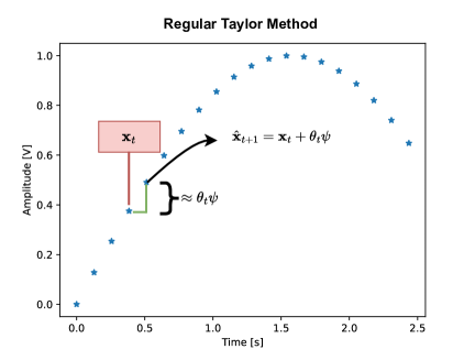
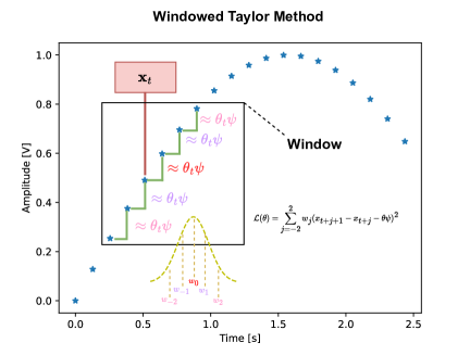
Figure 7: Taylor Method

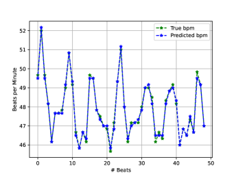
Figure 8: True hr vs. Reconstructed hr over time

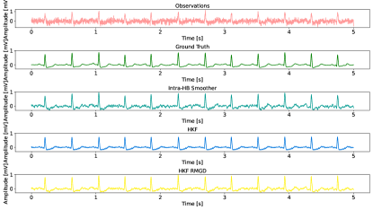
(a) Patient 0 - Proprietary

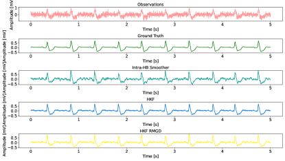
(b) Patient 1 - Proprietary

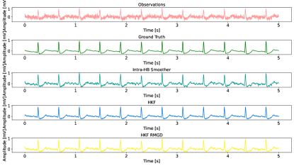
(c) Patient 2 - Proprietary

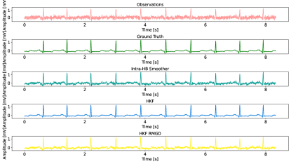
(d) Patient 100 - MIT-BIH

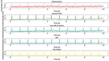
(e) Patient 101 - MIT-BIH

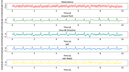
(f) Patient 102 - MIT-BIH

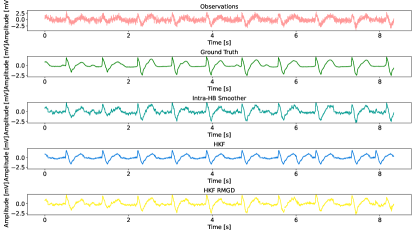
(g) Patient 107 - MIT-BIH

Figure 9: Sample of Consecutive hb

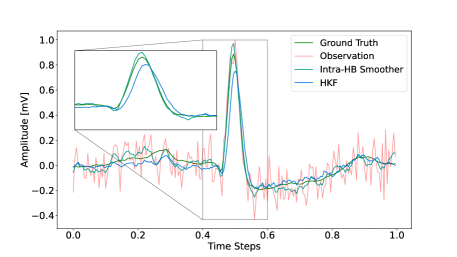
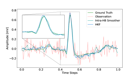
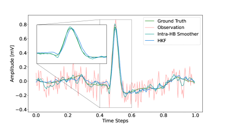
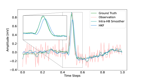
Figure 10: Single hb - Patient 0 - Proprietary

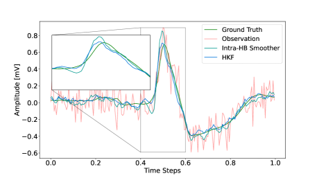
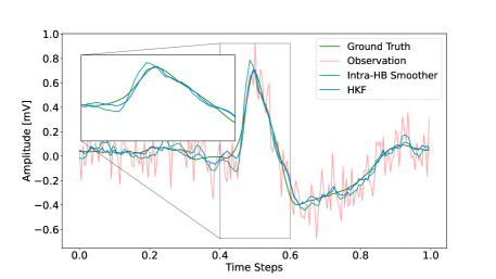
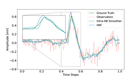
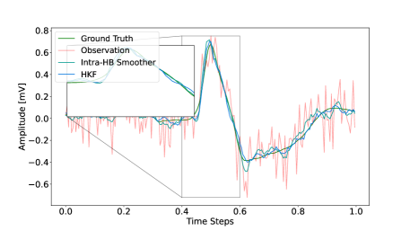
Figure 11: Single hb for patient 1 - Proprietary

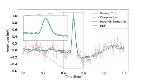
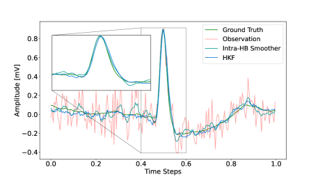
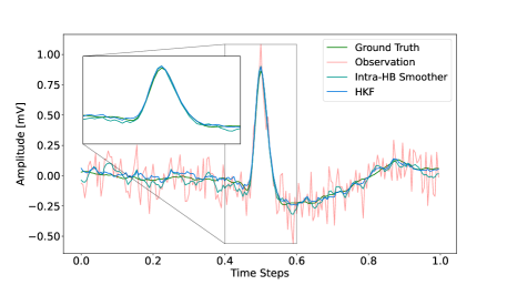
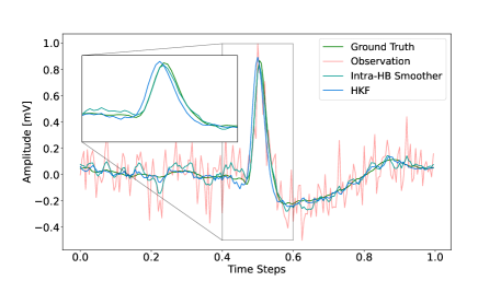
Figure 12: Single hb - Patient 2 - Proprietary

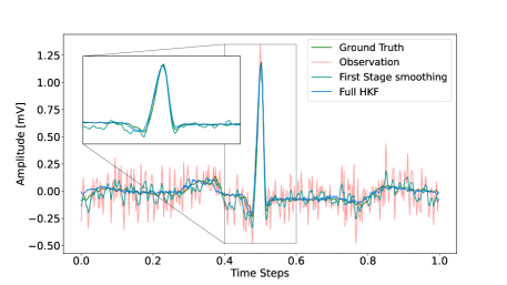
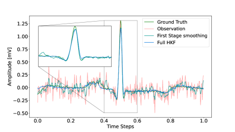
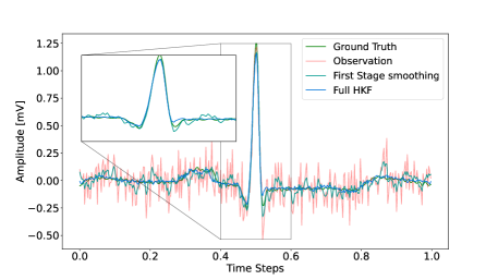
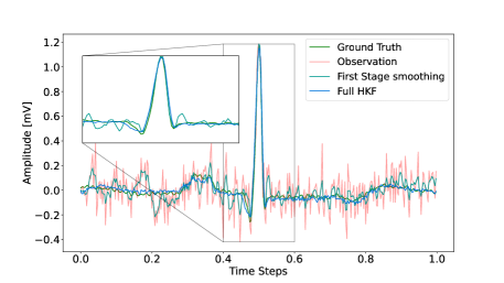
Figure 13: Single hb - Patient 100 - MIT-BIH

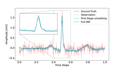
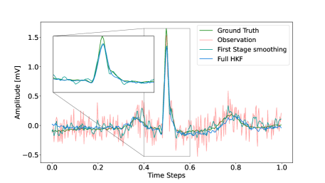
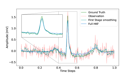
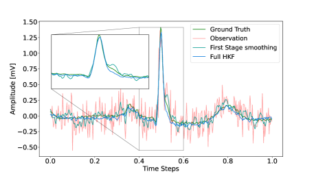
Figure 14: Single hb - Patient 101 - MIT-BIH

References

- [1] T. Locher, G. Revach, N. Shlezinger, R. J. G. van Sloun, and R. Vullings, “Hierarchical Filtering with Online Learned Priors for ECG Denoising,” in ICASSP 2023 - 2023 IEEE International Conference on Acoustics, Speech and Signal Processing (ICASSP), 2023, pp. 1–5.
- [2] Y. Bai, C. Tompkins, N. Gell, D. Dione, T. Zhang, and W. Byun, “Comprehensive comparison of Apple Watch and Fitbit monitors in a free-living setting,” PLoS One, vol. 16, no. 5, p. e0251975, 2021.
- [3] F. Sana, E. M. Isselbacher, J. P. Singh, E. K. Heist, B. Pathik, and A. A. Armoundas, “Wearable devices for ambulatory cardiac monitoring: Jacc state-of-the-art review.” Journal of the American College of Cardiology, vol. 75 13, pp. 1582–1592, 2020.
- [4] N. H. Service. (2021) Electrocardiogram. [Online]. Available: https://www.nhs.uk/conditions/electrocardiogram/
- [5] ——. (2021) Arrhythmia. [Online]. Available: https://www.nhs.uk/conditions/arrhythmia/
- [6] I. Amer-Wåhlin, C. Hellsten, H. Norén, H. Hagberg, A. Herbst, I. Kjellmer, H. Lilja, C. Lindoff, M. Månsson, L. Mårtensson et al., “Cardiotocography only versus cardiotocography plus st analysis of fetal electrocardiogram for intrapartum fetal monitoring: a swedish randomised controlled trial,” The Lancet, vol. 358, no. 9281, pp. 534–538, 2001.
- [7] N. H. Service. (2019) Heart attack. [Online]. Available: https://www.nhs.uk/conditions/heart-attack/
- [8] N. A. MACLACHLAN, J. A. SPENCER, K. HARDING, and S. Arulkumaran, “Fetal acidaemia, the cardiotocograph and the t/qrs ratio of the fetal ecg in labour,” BJOG: An International Journal of Obstetrics & Gynaecology, vol. 99, no. 1, pp. 26–31, 1992.
- [9] T. Kazmi, F. Radfer, and S. Khan, “ST Analysis of the fetal ECG, as an adjunct to fetal heart rate monitoring in labour: a review,” Oman medical journal, vol. 26, no. 6, p. 459, 2011.
- [10] A. Gruetzmann, S. Hansen, and J. Müller, “Novel dry electrodes for ECG monitoring,” Physiol. Meas., vol. 28, pp. 1375–1390, 2007.
- [11] J. Bailey et al., “Recommendations for standardization and specifications in automated electrocardiography: Bandwith and digital signal processing,” Circulation, vol. 81, pp. 730–739, 1990.
- [12] A. Velayudhan and S. Peter, “Noise analysis and different denoising techniques of ecg signal-a survey,” IOSR journal of electronics and communication engineering, vol. 1, no. 1, pp. 40–44, 2016.
- [13] S. Chatterjee, R. S. Thakur, R. N. Yadav, L. Gupta, and D. K. Raghuvanshi, “Review of noise removal techniques in ECG signals,” IET Signal Processing, vol. 14, no. 9, pp. 569–590, 2020.
- [14] H. Y. Mir and O. Singh, “ECG denoising and feature extraction techniques – a review,” Journal of Medical Engineering & Technology, vol. 45, no. 8, pp. 672–684, 2021.
- [15] Z. Zhang and X. Yang, “Review of ECG data feature processing and classification,” in International Conference on Biomedical and Intelligent Systems (IC-BIS 2022), vol. 12458, International Society for Optics and Photonics. SPIE, 2022, p. 124582S.
- [16] P. M. Tripathi, A. Kumar, R. Komaragiri, and M. Kumar, “A review on computational methods for denoising and detecting ECG signals to detect cardiovascular diseases,” Archives of Computational Methods in Engineering, pp. 1–40, 2021.
- [17] Y. LeCun, Y. Bengio, and G. Hinton, “Deep learning,” Nature, vol. 521, no. 7553, p. 436, 2015.
- [18] C. T. Arsene, R. Hankins, and H. Yin, “Deep Learning Models for Denoising ECG Signals,” in 2019 27th European Signal Processing Conference (EUSIPCO), 2019, pp. 1–5.
- [19] K. Antczak, “Deep recurrent neural networks for ECG signal denoising,” arXiv preprint arXiv:1807.11551, 2018.
- [20] H.-T. Chiang, Y.-Y. Hsieh, S.-W. Fu, K.-H. Hung, Y. Tsao, and S.-Y. Chien, “Noise reduction in ecg signals using fully convolutional denoising autoencoders,” IEEE Access, vol. 7, pp. 60 806–60 813, 2019.
- [21] E. Fotiadou and R. Vullings, “Multi-Channel Fetal ECG Denoising With Deep Convolutional Neural Networks,” Frontiers in Pediatrics, vol. 8, 2020.
- [22] P. Singh and G. Pradhan, “A New ECG Denoising Framework Using Generative Adversarial Network,” IEEE/ACM Transactions on Computational Biology and Bioinformatics, vol. 18, no. 2, pp. 759–764, 2021.
- [23] A. Rasti-Meymandi and A. Ghaffari, “A deep learning-based framework For ECG signal denoising based on stacked cardiac cycle tensor,” Biomedical Signal Processing and Control, vol. 71, p. 103275, 2022.
- [24] M. A. Kabir and C. Shahnaz, “Denoising of ECG signals based on noise reduction algorithms in EMD and wavelet domains,” Biomedical Signal Processing and Control, vol. 7, no. 5, pp. 481–489, 2012.
- [25] N. E. Huang, Z. Shen, S. R. Long, M. C. Wu, H. H. Shih, Q. Zheng, N.-C. Yen, C. C. Tung, and H. H. Liu, “The Empirical Mode Decomposition and the Hilbert Spectrum for Nonlinear and Non-Stationary Time Series Analysis,” Proceedings: Mathematical, Physical and Engineering Sciences, vol. 454, no. 1971, pp. 903–995, 1998.
- [26] B. Weng, M. Blanco-Velasco, and K. E. Barner, “ECG denoising based on the empirical mode decomposition,” in 2006 international conference of the IEEE engineering in medicine and biology society. IEEE, 2006, pp. 1–4.
- [27] Y. Lu, J. Yan, and Y. Yam, “Model-based ECG denoising using empirical mode decomposition,” in 2009 IEEE International Conference on Bioinformatics and Biomedicine. IEEE, 2009, pp. 191–196.
- [28] D. Zhang, S. Wang, F. Li, S. Tian, J. Wang, X. Ding, and R. Gong, “An efficient ECG denoising method based on empirical mode decomposition, sample entropy, and improved threshold function,” Wireless Communications and Mobile Computing, vol. 2020, pp. 1–11, 2020.
- [29] I. Daubechies, Ten lectures on wavelets. SIAM, 1992.
- [30] M. Shensa, “The discrete wavelet transform: wedding the a trous and Mallat algorithms,” IEEE Transactions on Signal Processing, vol. 40, no. 10, pp. 2464–2482, 1992.
- [31] J. Gilles, “Empirical Wavelet Transform,” IEEE Transactions on Signal Processing, vol. 61, no. 16, pp. 3999–4010, 2013.
- [32] O. Sayadi and M. B. Shamsollahi, “ECG denoising with adaptive bionic wavelet transform,” in 2006 International Conference of the IEEE Engineering in Medicine and Biology Society. IEEE, 2006, pp. 6597–6600.
- [33] M. Alfaouri and K. Daqrouq, “ECG signal denoising by wavelet transform thresholding,” American Journal of applied sciences, vol. 5, no. 3, pp. 276–281, 2008.
- [34] M. Ayat, M. B. Shamsollahi, B. Mozaffari, and S. Kharabian, “ECG denoising using modulus maxima of wavelet transform,” in 2009 Annual International Conference of the IEEE Engineering in Medicine and Biology Society, 2009, pp. 416–419.
- [35] G. Georgieva-Tsaneva and K. Tcheshmedjiev, “Denoising of electrocardiogram data with methods of wavelet transform,” in International Conference on Computer Systems and Technologies, vol. 13, no. 1, 2013, pp. 9–16.
- [36] P. Singh, G. Pradhan, and S. Shahnawazuddin, “Denoising of ECG signal by non-local estimation of approximation coefficients in DWT,” Biocybernetics and Biomedical Engineering, vol. 37, no. 3, pp. 599–610, 2017.
- [37] R. E. Kalman, “A new approach to linear filtering and prediction problems,” Journal of Basic Engineering, vol. 82, no. 1, pp. 35–45, 1960.
- [38] R. Sameni, M. B. Shamsollahi, C. Jutten, and G. D. Clifford, “A Nonlinear Bayesian Filtering Framework for ECG Denoising,” IEEE Transactions on Biomedical Engineering, vol. 54, no. 12, pp. 2172–2185, 2007.
- [39] O. Sayadi and M. B. Shamsollahi, “ECG Denoising and Compression Using a Modified Extended Kalman Filter Structure,” IEEE Transactions on Biomedical Engineering, vol. 55, no. 9, pp. 2240–2248, 2008.
- [40] R. Vullings, B. de Vries, and J. W. M. Bergmans, “An Adaptive Kalman Filter for ECG Signal Enhancement,” IEEE Transactions on Biomedical Engineering, vol. 58, no. 4, pp. 1094–1103, 2011.
- [41] H. D. Hesar and M. Mohebbi, “An Adaptive Kalman Filter Bank for ECG Denoising,” IEEE Journal of Biomedical and Health Informatics, vol. 25, no. 1, pp. 13–21, 2021.
- [42] M. A. Ouali, K. Chafaa, M. Ghanai, L. M. Lorente, and D. B. Rojas, “ECG denoising using extended Kalman filter,” in 2013 International Conference on Computer Applications Technology (ICCAT), 2013, pp. 1–6.
- [43] R. A. Wildhaber, N. Zalmai, M. Jacomet, and H.-A. Loeliger, “Windowed State-Space Filters for Signal Detection and Separation,” IEEE Transactions on Signal Processing, vol. 66, no. 14, pp. 3768–3783, 2018.
- [44] R. A. Wildhaber, “Localized State Space and Polynomial Filters with Applications in Electrocardiography,” Ph.D. dissertation, ETH Zurich, Zurich, Switzerland, 2019.
- [45] R. A. Wildhaber, E. Ren, F. Waldmann, and H.-A. Loeliger, “Signal Analysis Using Local Polynomial Approximations,” in 2020 28th European Signal Processing Conference (EUSIPCO), 2021, pp. 2239–2243.
- [46] R. M. Evaristo, A. M. Batista, R. L. Viana, K. C. Iarosz, J. D. Szezech Jr, and M. F. de Godoy, “Mathematical model with autoregressive process for electrocardiogram signals,” Communications in Nonlinear Science and Numerical Simulation, vol. 57, pp. 415–421, 2018.
- [47] F. Huang, T. Qin, L. Wang, H. Wan, and J. Ren, “An ecg signal prediction method based on arima model and dwt,” in 2019 IEEE 4th Advanced Information Technology, Electronic and Automation Control Conference (IAEAC), vol. 1. IEEE, 2019, pp. 1298–1304.
- [48] S. Särkkä, Bayesian filtering and smoothing. Cambridge University Press, 2013, no. 3.
- [49] P. McSharry, G. Clifford, L. Tarassenko, and L. Smith, “A dynamical model for generating synthetic electrocardiogram signals,” IEEE Transactions on Biomedical Engineering, vol. 50, no. 3, pp. 289–294, 2003.
- [50] H. E. Rauch, F. Tung, and C. T. Striebel, “Maximum likelihood estimates of linear dynamic systems,” AIAA Journal, vol. 3, no. 8, pp. 1445–1450, 1965.
- [51] O. College. Illustration from Anatomy & Physiology. [Online]. Available: http://cnx.org/content/col11496/1.6/
- [52] D. Kilpatrick and P. Johnston, “Origin of the electrocardiogram,” IEEE Engineering in Medicine and Biology Magazine, vol. 13, no. 4, pp. 479–486, 1994.
- [53] J. Allen and A. Murray, “Assessing ECG signal quality on a coronary care unit,” Physiological measurement, vol. 17, no. 4, p. 249, 1996.
- [54] Y. Bar-Shalom, X. R. Li, and T. Kirubarajan, Estimation with applications to tracking and navigation: theory algorithms and software. John Wiley & Sons, 2004.
- [55] G. B. Giannakis, “Cyclostationary signal analysis,” in Digital Signal Processing Handbook, 1998, vol. 31, pp. 1–17.
- [56] I. I. Christov, “Real time electrocardiogram QRS detection using combined adaptive threshold,” Biomedical engineering online, vol. 3, no. 1, pp. 1–9, 2004.
- [57] L. Sathyapriya, L. Murali, and T. Manigandan, “Analysis and detection R-peak detection using Modified Pan-Tompkins algorithm,” in 2014 IEEE International Conference on Advanced Communications, Control and Computing Technologies. IEEE, 2014, pp. 483–487.
- [58] F. Waldmann, C. Baeriswyl, R. Andonie, and R. A. Wildhaber, “Onset Detection of Pulse-Shaped Bioelectrical Signals Using Linear State Space Models,” Current Directions in Biomedical Engineering, vol. 8, no. 2, pp. 101–104, 2022.
- [59] P. J. M. Fard, M. Moradi, and M. Tajvidi, “A novel approach in R peak detection using hybrid complex wavelet (HCW),” International Journal of Cardiology, vol. 124, no. 2, pp. 250–253, 2008.
- [60] Y. Zou, J. Han, S. Xuan, S. Huang, X. Weng, D. Fang, and X. Zeng, “An Energy-Efficient Design for ECG Recording and R-Peak Detection Based on Wavelet Transform,” IEEE Transactions on Circuits and Systems II: Express Briefs, vol. 62, no. 2, pp. 119–123, 2015.
- [61] J. Laitala, M. Jiang, E. Syrjälä, E. K. Naeini, A. Airola, A. M. Rahmani, N. D. Dutt, and P. Liljeberg, “Robust ECG R-peak detection using LSTM,” in Proceedings of the 35th annual ACM symposium on applied computing, 2020, pp. 1104–1111.
- [62] P. Group. BioSPPy. [Online]. Available: https://github.com/PIA-Group/BioSPPy
- [63] W. A. Engelse and C. Zeelenberg, “A single scan algorithm for QRS-detection and feature extraction,” Computers in cardiology, vol. 6, no. 1979, pp. 37–42, 1979.
- [64] A. Lourenço, H. Silva, P. Leite, R. Lourenço, and A. L. Fred, “Real Time Electrocardiogram Segmentation for Finger based ECG Biometrics.” in Biosignals, 2012, pp. 49–54.
- [65] Z. Ghahramani and G. E. Hinton, “Parameter estimation for linear dynamical systems,” University of Totronto, Dept. of CS, Tech. Rep. CRG-TR-96-2, 02 1996.
- [66] J. Dauwels, A. Eckford, S. Korl, and H.-A. Loeliger, “Expectation maximization as message passing-part I: Principles and Gaussian messages,” arXiv preprint arXiv:0910.2832, 2009.
- [67] Sophocles J. Orfanidis, Applied Optimum Signal Processing. Rutgers University, 2018.
- [68] P. De Jong, “The likelihood for a state space model,” Biometrika, vol. 75, no. 1, pp. 165–169, 1988.
- [69] S. Bonnabel, “Stochastic gradient descent on Riemannian manifolds,” IEEE Transactions on Automatic Control, vol. 58, no. 9, pp. 2217–2229, 2013.
- [70] S. Sra and R. Hosseini, “Conic Geometric Optimization on the Manifold of Positive Definite Matrices,” SIAM Journal on Optimization, vol. 25, no. 1, pp. 713–739, 2015.
- [71] J. M. Lee, Introduction to Riemannian manifolds. Springer, 2018, vol. 176.
- [72] R. Bhatia, “Positive definite matrices, princeton ser,” Appl. Math., Princeton University Press, Princeton, NJ, 2007.
- [73] V. Arsigny, P. Fillard, X. Pennec, and N. Ayache, “Geometric means in a novel vector space structure on symmetric positive-definite matrices,” SIAM journal on matrix analysis and applications, vol. 29, no. 1, pp. 328–347, 2007.
- [74] Z. Lin, “Riemannian Geometry of Symmetric Positive Definite Matrices via Cholesky Decomposition,” SIAM Journal on Matrix Analysis and Applications, vol. 40, no. 4, pp. 1353–1370, 2019.
- [75] G. Revach, X. Ni, N. Shlezinger, R. J. G. van Sloun, and Y. C. Eldar, “RTSNet: Learning to Smooth in Partially Known State-Space Models,” CoRR, vol. abs/2110.04717, 2023, Accepted to IEEE Transactions on Signal Processing.
- [76] G. Revach, N. Shlezinger, X. Ni, A. L. Escoriza, R. J. G. van Sloun, and Y. C. Eldar, “KalmanNet: Neural Network Aided Kalman Filtering for Partially Known Dynamics,” IEEE Transactions on Signal Processing, vol. 70, pp. 1532–1547, 2022.
- [77] A. L. Goldberger, L. A. Amaral, L. Glass, J. M. Hausdorff, P. C. Ivanov, R. G. Mark, J. E. Mietus, G. B. Moody, C.-K. Peng, and H. E. Stanley, “Physiobank, physiotoolkit, and physionet: components of a new research resource for complex physiologic signals,” circulation, vol. 101, no. 23, pp. e215–e220, 2000.