LQGNet: Hybrid Model-Based and Data-Driven Linear Quadratic Stochastic Control

Abstract

Stochastic control deals with finding an optimal control signal for a dynamical system in a setting with uncertainty, playing a key role in numerous applications. The lqg (lqg) is a widely-used setting, where the system dynamics is represented as a lg ss (ss) model, and the objective function is quadratic. For this setting, the optimal controller is obtained in closed form by the separation principle. However, in practice, the underlying system dynamics often cannot be faithfully captured by a fully known lg ss model, limiting its performance. Here, we present ln, a stochastic controller that leverages data to operate under partially known dynamics. ln augments the state tracking module of separation-based control with a dedicated trainable algorithm. The resulting system preserves the operation of classic lqg control while learning to cope with partially known ss models without having to fully identify the dynamics. We empirically show that ln outperforms classic stochastic control by overcoming mismatched ss models.

Index Terms—  Stochastic control, lqg, dl.

1 Introduction

Stochastic optimal control is a sub-field of mathematical optimization with applications spanning from operations research to physical sciences and engineering, including aerospace, vehicular systems, and robotics [1]. Stochastic control consdiers dynamical system under the existence of uncertainty, either in its evolution or in its observations.The aim is to find an optimal control signal for a given objective function. In the fundamental lqg setting [2], e the system dynamics obey a lg ss model, and the controller should minimize a quadratic objective. The optimal lqg controller follows the separation principle [3, 4], where state estimation is decoupled from control, and it comprises a kf (kf) followed by a conventional lqr (lqr) [5].

While lqg control is simple and tractable, it relies on the ability to faithfully describe the dynamics as a fully known lg ss model. In practice, ss models are often approximations of the system’s true dynamics, while its stochasticity can be non-Gaussian. The presence of such mismatched domain knowledge notably affects the performance of classical mb policies.

To overcome the drawbacks of oversimplified modeling, one can resort to learning. The main learning-based approach in sequential decision making and control is rl (rl) [6, 7] where an agent is trained via experience-driven autonomous learning to maximize a reward [8]. The growing popularity of model-agnostic dnn and their empirical success in various tasks involving complex data, such as visual and language data, has led to a growing interest in deep rl [9]. Deep rl systems based on black-box dnn were proposed for implementing controllers for various tasks, including robotics and vehicular systems [10, 11]. Despite their success, these architectures cannot naturally incorporate the domain knowledge available in partially known ss models, are complex and difficult to train, and lack the interpretability of mb methods [12]. An alternative approach uses dnn to extract features processed with model-based methods [13, 14, 15]. This approach still requires one to impose a fully known ss model of the features, motivating the incorporation of deep learning into classic controllers to bypass the need to fully characterize the dynamics.

In this work, we propose ln, a hybrid stochastic controller designed via model-based deep learning [12, 16]. ln preserves the structure of the optimal lqg policy, while operating in partially known settings. We adopt the recent kn architecture [17], which implements a trainable kf, in a separation-based controller. The resulting ln architecture utilizes the available domain knowledge by exploiting the system’s description as a ss model, thus preserving the simplicity and interpretability of the mb policy while leveraging data to overcome partial information and model mismatches. By converting the optimal mb lqg controller into a trainable discriminative algorithm [18] our ln learns to control in an e2e manner. We empirically demonstrate that ln approaches the performance of the optimal lqg policy with fully known ss models, and notably outperforms it in the presence of mismatches.

The rest of this paper is organized as follows: Section 2 reviews the ss model and details the lqg control task. Section 3 presents ln, which is evaluated in Section 4.

2 System Model and Preliminaries

As a preliminary step to deriving ln (ln), we describe in the describes the system model in Subsection 2.1. Subsection 2.2 the formulates the dd lqg control task in partially known ss models, and Subsection 2.3 reviews basics in optimal mb lqg control.

2.1 Dynamical System Model

We consider dynamic systems characterized by a ss model in discrete-time $t\in\mathbb{Z}$. This ss model describes the relationship between a state vector ${\mathbf{x}}_{t}\in\mathbb{R}^{m}$, an input control signal ${\mathbf{u}}_{t}\in\mathbb{R}^{q}$, and the noisy observations ${\mathbf{y}}_{t}\in\mathbb{R}^{n}$, at each time instance $t$. We focus on lg models, given by

$$\mathbf{x}_{t} ={\mathbf{F}}\cdot{\mathbf{x}}_{t-1}+{\mathbf{G}}\cdot{\mathbf{u}}_{t-1}+{\mathbf{w}}_{t}, \mathbf{w}_{t}\sim\mathcal{N}\left(\mathbf{0},\mathbf{W}\right),$$ (1a)

$$\mathbf{y}_{t} ={\mathbf{H}}\cdot\mathbf{x}_{t}+\mathbf{v}_{t}, \mathbf{v}_{t}\sim\mathcal{N}\left(\mathbf{0},\mathbf{V}\right).$$ (1b)

Here, ${\mathbf{F}}\in\mathbb{R}^{m\times m}$, ${\mathbf{G}}\in\mathbb{R}^{m\times q}$, and ${\mathbf{H}}\in\mathbb{R}^{n\times m}$ are the evolution, control, and observation (emission) matrices, respectively, and ${\mathbf{w}}_{t},{\mathbf{v}}_{t}$ are awgn signals with covarainces $\mathbf{W},\mathbf{V}$, respectively.

2.2 Data Driven Stochastic Control Task

The stochastic control task considers the optimization of a policy $\psi:\mathbb{R}^{n}\mapsto\mathbb{R}^{q}$, which maps a noisy observation signal ${\mathbf{y}}_{t}$ into a control signal ${\mathbf{u}}_{t}$, under quadratic control loss. Over a finite-horizon of $\mathrm{T}$ time steps, the loss is given by

$${\mathbf{J}}(\psi)=\tilde{{\mathbf{x}}}_{\mathrm{T}}^{\top}\mathbf{Q}_{\mathrm{T}}\tilde{{\mathbf{x}}}_{\mathrm{T}}+\sum_{t=0}^{\mathrm{T}-1}\left(\tilde{{\mathbf{x}}}_{t}^{\top}\mathbf{Q}_{\tilde{{\mathbf{x}}}}\tilde{{\mathbf{x}}}_{t}+\tilde{{\mathbf{u}}}_{t}^{\top}\mathbf{R}_{\tilde{{\mathbf{u}}}}\tilde{{\mathbf{u}}}_{t}\right).$$ (2)

The loss (2) balances the stability of the closed-loop system and the aggressiveness of control. Here, $\tilde{{\mathbf{u}}}_{t}$ and $\tilde{{\mathbf{x}}}_{t}$ are the deviations of ${\mathbf{u}}_{t}$ and ${\mathbf{x}}_{t}$, respectively, from predefined target values. The former is typically set to zero, while the latter is a desired state that depends on the regulation problem. The matrices $\mathbf{Q}_{\tilde{{\mathbf{x}}}},\mathbf{Q}_{\mathrm{T}}\succeq 0$, and $\mathbf{R}_{\tilde{{\mathbf{u}}}}\succ 0$ are predefined weighting costs for state, final state, and input control, respectively. While we assume to have access to a (possibly mismatched) estimate of the ss design matrices ${\mathbf{F}},{\mathbf{G}}$, ${\mathbf{H}}$, we do not assume prior knowledge of the distribution of the noises.

To overcome this missing domain knowledge, we are given access to a simulator $\Gamma:\mathbb{R}^{q}\mapsto\mathbb{R}^{m}\times\mathbb{R}^{n}$ that emulates the underlying dynamics. The simulator allows generating random trajectories of inputs while measuring their observations and state values, i.e., $({\mathbf{y}}_{t},{\mathbf{x}}_{t})=\Gamma({\mathbf{u}}_{t-1})$.

2.3 Optimal LQG Control

lqg is one of the most fundamental optimal control frameworks [2]. It considers dynamics with a lg ss model as in (1) with a quadratic objective as in (2). For such setting, (1), the separation principle [3, 5] applies, and the optimal policy $\psi^{\ast}$ which minimizes (2) can be decomposed into two separate modules: a mse (mse) optimal state estimator, namely the kf, followed by full-state optimal lqr. Both modules, detailed next, require full knowledge of the ss model parameters.

2.3.1 Kalman filter - mse optimal state estimator

The kf is an efficient linear recursive state estimator, which for every time step $t$ produces an estimate $\hat{{\mathbf{x}}}_{t}$ for ${\mathbf{x}}_{t}$, based on all previous and current observations $\{{\mathbf{y}}_{\tau}\}_{\tau\leq t}$. It can be described as a two-step procedure; prediction and update, that uses only the new observation and the previous estimate as sufficient statistics to compute first and second order moments. The prediction is given by

$$\hat{\mathbf{x}}_{t\left|t-1\right.} \!=\!\mathbf{F}{\hat{\mathbf{x}}_{t-1}}\!+\!{\mathbf{G}}{\mathbf{u}}_{t-1},\hskip 5.69046pt\boldsymbol{\Sigma}_{t\left|t-1\right.}\!=\!\mathbf{F}\boldsymbol{\Sigma}_{t-1}\mathbf{F}^{\top}\!+\!\mathbf{W},$$ (3a)

$$\hat{\mathbf{y}}_{t\left|t-1\right.} \!=\!\mathbf{H}{\hat{\mathbf{x}}_{t\left|t-1\right.}},\hskip 38.41139pt\mathbf{S}_{t}\!=\!\mathbf{H}\boldsymbol{\Sigma}_{t\left|t-1\right.}\mathbf{H}^{\top}\!+\!\mathbf{V},$$ (3b)

and the update is given by

$$\hat{\mathbf{x}}_{t} =\hat{\mathbf{x}}_{t\left|t-1\right.}+{\mathbf{K}}_{t}\cdot\Delta\mathbf{y}_{t},\quad\Delta\mathbf{y}_{t}=\mathbf{y}_{t}-\hat{\mathbf{y}}_{t\left|t-1\right.},$$ (4a)

$${\mathbf{K}}_{t} ={\boldsymbol{\Sigma}}_{t\left|t-1\right.}{\mathbf{H}^{\top}}{\mathbf{S}}^{-1}_{t},\quad{\boldsymbol{\Sigma}}_{t}\!=\!{\boldsymbol{\Sigma}}_{t\left|t-1\right.}\!-\!{\mathbf{K}}_{t}{\mathbf{S}}_{t}{\mathbf{K}}^{\top}_{t}.$$ (4b)

Here, ${\mathbf{K}}_{t}$ is the kg (kg), computed recursively based on tracking the second-order moments of the signals.

2.3.2 Optimal LQR policy

For the system in (1) with known $({\mathbf{F}},{\mathbf{G}})$, the optimal control input is given by

$${\mathbf{u}}_{t}\!=\!-{\mathbf{L}}_{t}\hat{{\mathbf{x}}}_{t},\hskip 8.5359pt{\mathbf{L}}_{t}\!=\!\left[{\mathbf{R}}_{\tilde{{\mathbf{u}}}}+{\mathbf{G}}^{\top}{\mathbf{P}}_{t+1}{\mathbf{G}}\right]^{-1}{\mathbf{G}}^{\top}{\mathbf{P}}_{t+1}{\mathbf{F}}.$$ (5)

${\mathbf{L}}_{t}$ is control gain and $\mathbf{P}_{t}$ is the solution to the dare [19], computed as

$${\mathbf{P}}_{t-1}={\mathbf{Q}}_{\tilde{{\mathbf{x}}}}+{\mathbf{F}}^{\top}{\mathbf{P}}_{t}{\mathbf{F}}-{\mathbf{F}}^{\top}{\mathbf{P}}_{t}{\mathbf{G}}\cdot{\mathbf{L}}_{t-1}.$$ (6)

The above controller coincides with the lqr policy, that minimizes the quadratic objective for lg ss models where one has a noise-free observation of the state.

3 LQGNet

Next, we present ln, which learns to implement lqg control under the considered partially known ss model. We begin by detailing the architecture of ln in Subsection 3.1, after which we describe the training procedure and provide a discussion in Subsections 3.2-3.3, respectively.

3.1 LQGNet Architecture

The optimal lqg controller detailed in Subsection 2.3 requiresfull access to the ss model (1). While the design matrices ${\mathbf{F}},{\mathbf{G}}$, ${\mathbf{H}}$ are assumed to be partially known, the distributions of the noise signals are not known at all. Consequently, to cope with this missing knowledge without imposing a model and estimating the statistics of the noise signals, ln augments the state estimator with deep learning.

Since the lqg optimal controller employs the kf for state estimation, we replace it with our recently proposed kn architecture [17]. kn is particularly suitable here, as it preserves the flow and interpretable nature of the kf [20]. While the mb kf requires the noise statistics to formulate the kg ${\mathbf{K}}_{t}$ (4b), kn uses a trainable rnn (rnn) to compute it, bypassing the need to impose a model on the noises. More specifically, kn predicts the first order moments using the design matrices, as in (3), and then updates using its learned (surrogate) kg, as in (4a). The state estimate produced by kn is then processed by the mb lqr (5) and the gain ${\mathbf{L}}_{t}$ using the available (though possibly approximated) design matrices, where the noise covarince matrices are not required. The resulting architecture is illustrated in Fig. 1.

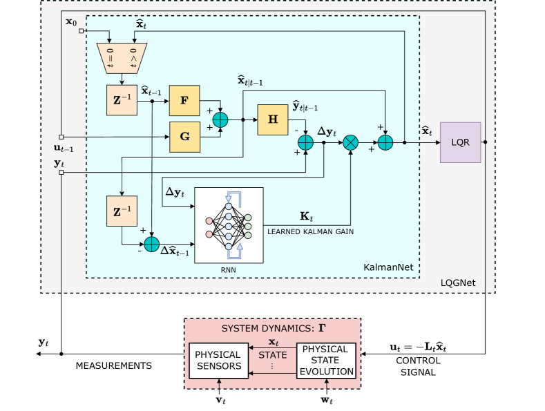
Fig. 1: LQGNet block diagram.

3.2 Training Algorithm

The trainable parameters of ln are the weights of the internal rnn used to compute the kg, denoted $\mathbf{\Theta}$. In principle, one can use the data simulator $\Gamma$ to train the state estimator separately from the control task, i.e., to minimize the state estimate mse in a supervised manner [17], or to optimize its internal predictions in an unsupervised manner [21]. However, inspired by rl [8], since the lqr policy (5) uses the possibly mismatched design matrices, we aim to train the overall system in an e2e manner, based on the quadratic control objective (2). By doing so, we leverage data to jointly cope with mismatches in both the state estimate and the regulator.

To formulate the training loss, we use ${\mathbf{J}}_{\Gamma}(\mathbf{\Theta})$ to denote the objective (2) evaluated when applying ln with parameters $\mathbf{\Theta}$ to control the dynamics of the simulator $\Gamma$. The random nature of the simulator indicates that restarting it multiple times yields different trajectories. We can thus formulate the regularized lqg loss as

$$\mathcal{L}_{\Gamma}\left(\mathbf{\Theta}\right)={\mathbf{J}}_{\Gamma}(\mathbf{\Theta})+\gamma\cdot\|\mathbf{\Theta}\|_{2}^{2},$$ (7)

where $\gamma>0$ is a regularization coefficient. By (5), the input ${\mathbf{u}}_{t}$ is differentiable with respect to the state estimate $\hat{{\mathbf{x}}}_{t}$, which is in turn differentiable with respect to $\mathbf{\Theta}$ [17]. Consequently, the loss in (7) is differentiable, allowing to train ln e2e as a discriminative model [18] via gradient-based learning. The resulting training procedure is summarized in Algorithm 1.

Init : Randomize $\mathbf{\Theta}$
Fix learning rate $\mu>0$ and iterations $i_{\max}$

Input : Simulator $\Gamma$

1 for $i=0,1,\ldots,i_{\max}-1$ do

2      Simulate LQGNet with parameters $\mathbf{\Theta}$ using $\Gamma$;

3       Update $\mathbf{\Theta}\leftarrow\mathbf{\Theta}-\mu\cdot\nabla_{\mathbf{\Theta}}\mathcal{L}_{\Gamma}(\mathbf{\Theta})$;

4      

return $\mathbf{\Theta}$

Algorithm 1 Training LQGNet

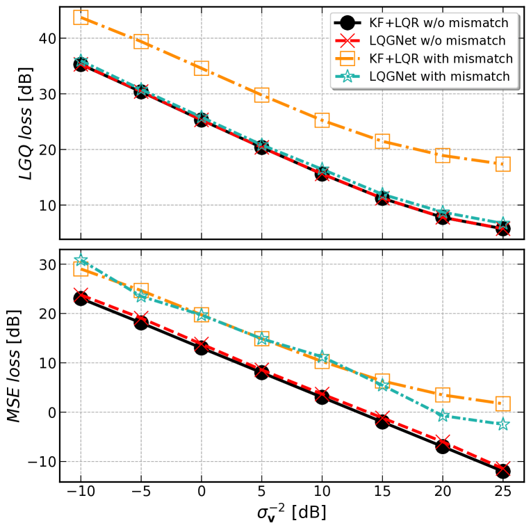
(a) Mismatched state evolution

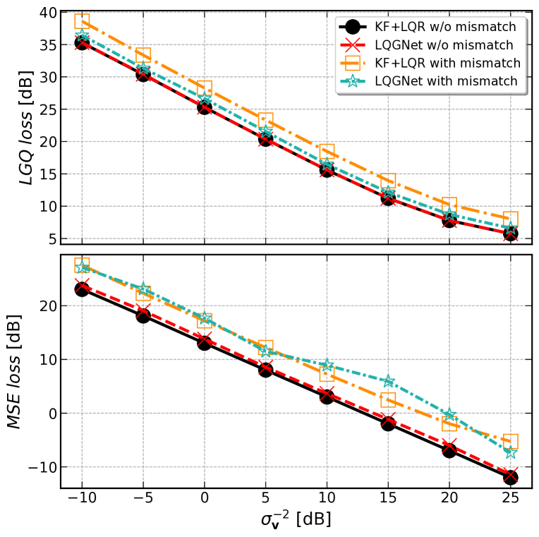
(b) Mismatched observations

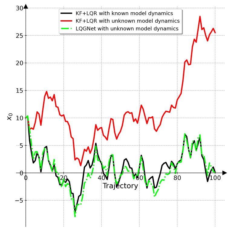
(c) Trajectory along a single state entry

Fig. 2: Control loss (upper) and state estimation mse (lower) with and without mismatches.

3.3 Discussion

ln is a hybrid mb/dd implementation of the optimal lqg controller. Comprising a trainable kf and the lqr policy, it preserves the interpretable and low-complexity operation of the mb controller. By augmenting the kg computation, which encapsulates the noise statistics, with an rnn, ln operates without imposing a model on the noise signals. The training procedure adapts ln based on the overall control objective, facilitating coping with mismatches in the ss model parameters. In particular, ln can overcome uncertainty by learning an alternative state estimate that yields high performance control, as demonstrated in Section 4.

ln gives rise to multiple possible extensions. For instance, while we focus on linear ss models, the proposed design can potentially be enhanced to account for non-linear dynamics [22]. Furthermore, it can be enhanced to account for alternative control objectives such as model predictive control, and utilize corresponding regulators such as emerging convex optimization control policies [23]. We leave these extensions for future investigation.

4 Empirical Evaluations

Next, we empirically study the performance of ln. We evaluate both the control objective (lqg loss (2)) and the state estimation mse for different levels of observation noise. Since it was derived from the optimal lqg controller, we compare it with the mb controller, i.e., kf-lqr, when operating with and without mismatches, Here, the noise signals obey the ss model in (1), with diagonal covariance matrices with an identical variance, i.e., $\mathbf{V}=\sigma_{{\mathbf{v}}}^{2}\mathbf{I}$, $\mathbf{W}=\sigma_{{\mathbf{w}}}^{2}\mathbf{I}$, and $\sigma_{{\mathbf{w}}}^{2}=\sigma_{{\mathbf{v}}}^{2}$. In the non-mismatched case, the dynamics also obey the ss model, with the design matrices

$${\mathbf{F}}=\left[\begin{array}[]{cc}1&1\\ 0&1\\ \end{array}\right];\quad{\mathbf{G}}=\left[\begin{array}[]{c}0\\ 1\\ \end{array}\right];\quad{\mathbf{H}}=\left[\begin{array}[]{cc}1&0\\ 0&1\\ \end{array}\right].$$ (8)

In the mismatched case the design matrices stay the same, but in the gt dynamics, from which the data was generated, either ${\mathbf{F}}$ or ${\mathbf{H}}$ are replaced by

$$\mathbf{R}_{\alpha}{\mathbf{F}},\quad\mathbf{R}_{\alpha}{\mathbf{H}},\quad\mathbf{R}_{\alpha}\!=\!\left[\begin{array}[]{cc}\cos{(\alpha)}&-\sin{(\alpha)}\\ \sin{(\alpha)}&\cos{(\alpha)}\\ \end{array}\right],$$ (11)

namely, rotated with $\alpha=20^{\circ}$.

The loss measures achieved by ln compared with mb kf-lqr are depicted in Fig. 2 for both full and partial model information. The mismatch in Fig. 2(a) is in the state-evolution ${\mathbf{F}}$, and the mismatch in Fig. 2(b) corresponds to the observation mapping ${\mathbf{H}}$. As expected, in the absence of mismatches, the optimal lqg controller achieves the lowest mse and lqg values, as it follows the separation principle for optimality. For the same setting, ln approaches the optimal mse and lqg performance. Even though ln is trained to minimize the lqg loss, it is not surprising that it achieves optimal performance in both lqg and mse metrics. Optimal control is approached because lqr and kf (i.e., lqe) are dual problems [24], which also indicates that ln learns to obey the separation principle when it is optimal.

Under the setting with partial (mismatched) model information, the lqg loss associated with the ln is notably better than its mb counterpart. However, ln does not accurately estimate the state here, achieving mse that is notably higher than the lower bound. The learned kg of ln induced by training on the lqg loss produces different state estimates than the mb controllers. However, these estimates, despite being inaccurate, enable the mismatched lqr controller to produce reliable inputs.

The result for the partial knowledge in the state-evolution in Fig. 2(a) is also reflected in Fig. 2(c), where a single trajectory of the first entry of ${\mathbf{x}}_{t}$ is presented. Here, the initial state is set to ${\mathbf{x}}_{0}=\left[10,0\right]^{\top}$ and $\sigma_{{\mathbf{w}}}^{2}=\sigma_{{\mathbf{v}}}^{2}=0\left[\textrm{dB}\right]$. We observe that despite the fact that ln operates with a mismatched state-evolution matrix ${\mathbf{F}}$, it controls the state to yield a trajectory that is closely similar to that achieved for the same setting using the optimal lqg controller. These results demonstrate the ability of ln to reliably learn from data to control partially known ss models.

5 Conclusions

In this work we presented ln, a hybrid mb and dd stochastic controller. Our design augments the optimal lqg controller with a deep learning component, using the recently proposed kn to overcome unknown noise distributions. We train ln e2e, such that it learns from data to overcome model mismatches. Our numerical study shows that ln approaches optimal control with both a full and partial ss model, and that it retains the simplicity and interpretability of its classic mb counterpart while implicitly learning to cope with mismatched dynamics.

References

- [1] A. Bryson, “Optimal control-1950 to 1985,” IEEE Control Syst. Mag., vol. 16, no. 3, pp. 26–33, 1996.
- [2] M. Athans, “The role and use of the stochastic linear-quadratic-gaussian problem in control system design,” IEEE Trans. Autom. Control, 1971.
- [3] T. Yoshikawa and H. Kobayashi, “Separation of estimation and control for decentralized stochastic control systems,” IFAC Proceedings Volumes, 1978.
- [4] T. Gunckel and G. F. Franklin, “A general solution for linear, sampled-data control,” 1963.
- [5] I. Gunckel, T. L. and G. F. Franklin, “A General Solution for Linear, Sampled-Data Control,” Journal of Basic Engineering, vol. 85, no. 2, pp. 197–201, 06 1963.
- [6] D. P. Bertsekas and J. N. Tsitsiklis, Neuro-dynamic programming, ser. Optimization and neural computation series. Athena Scientific, 1996, vol. 3. [Online]. Available: https://www.worldcat.org/oclc/35983505
- [7] R. S. Sutton and A. G. Barto, Reinforcement learning: An introduction. MIT press, 2018.
- [8] D. Silver, S. Singh, D. Precup, and R. S. Sutton, “Reward is enough,” Artif. Intell., vol. 299, p. 103535, 2021. [Online]. Available: https://doi.org/10.1016/j.artint.2021.103535
- [9] K. Arulkumaran, M. P. Deisenroth, M. Brundage, and A. A. Bharath, “Deep reinforcement learning: A brief survey,” IEEE Signal Process. Mag., vol. 34, no. 6, pp. 26–38, 2017.
- [10] S. Kuutti, R. Bowden, Y. Jin, P. Barber, and S. Fallah, “A survey of deep learning applications to autonomous vehicle control,” IEEE Trans. Intell. Transp. Syst., vol. 22, no. 2, pp. 712–733, 2020.
- [11] K. Zhang, J. Wang, X. Xin, X. Li, C. Sun, J. Huang, and W. Kong, “A survey on learning-based model predictive control: Toward path tracking control of mobile platforms,” Applied Sciences, vol. 12, no. 4, p. 1995, 2022.
- [12] N. Shlezinger, J. Whang, Y. C. Eldar, and A. G. Dimakis, “Model-based deep learning,” arXiv preprint arXiv:2012.08405, 2020.
- [13] T. Iwata and Y. Kawahara, “Controlling nonlinear dynamical systems with linear quadratic regulator-based policy networks in Koopman space,” in IEEE CDC, 2021, pp. 5086–5091.
- [14] J. Peralez and M. Nadri, “Deep learning-based Luenberger observer design for discrete-time nonlinear systems,” in IEEE CDC, 2021, pp. 4370–4375.
- [15] E. A. M. Perez and H. Iba, “Deep learning-based inverse modeling for predictive control,” IEEE Control Syst. Lett., vol. 6, pp. 956–961, 2021.
- [16] N. Shlezinger, Y. C. Eldar, and S. P. Boyd, “Model-based deep learning: On the intersection of deep learning and optimization,” arXiv preprint arXiv:2205.02640, 2022.
- [17] G. Revach, N. Shlezinger, X. Ni, A. L. Escoriza, R. J. G. van Sloun, and Y. C. Eldar, “KalmanNet: Neural network aided Kalman filtering for partially known dynamics,” IEEE Trans. Signal Process., vol. 70, pp. 1532–1547, 2022.
- [18] N. Shlezinger and T. Routtenberg, “Discriminative and generative learning for linear estimation of random signals [lecture notes],” arXiv preprint arXiv:2206.04432, 2022.
- [19] F. L. Lewis and V. L. Syrmos, Optimal Control, Third Edition. John Wiley and Sons, Inc., 2012.
- [20] I. Klein, G. Revach, N. Shlezinger, J. E. Mehr, R. J. G. van Sloun, and Y. C. Eldar, “Uncertainty in data-driven Kalman filtering for partially known state-space models,” in IEEE ICASSP, 2022.
- [21] G. Revach, N. Shlezinger, T. Locher, X. Ni, R. J. van Sloun, and Y. C. Eldar, “Unsupervised learned Kalman filtering,” in EUSIPCO, 2022.
- [22] E. Todorov and W. Li, “A generalized iterative LQG method for locally-optimal feedback control of constrained nonlinear stochastic systems,” in American Control Conference (ACC), 2005, pp. 300–306.
- [23] A. Agrawal, S. Barratt, S. Boyd, and B. Stellato, “Learning convex optimization control policies,” in Learning for Dynamics and Control. PMLR, 2020, pp. 361–373.
- [24] P. A. Blackmore and R. R. Bitmead, “Duality between the discrete-time Kalman filter and LQ control law,” IEEE Trans. Autom. Control, 1995.