MM-Align: Learning Optimal Transport-based Alignment Dynamics for Fast and Accurate Inference on Missing Modality Sequences

Abstract

Existing multimodal tasks mostly target at the complete input modality setting, i.e., each modality is either complete or completely missing in both training and test sets. However, the randomly missing situations have still been underexplored. In this paper, we present a novel approach named MM-Align to address the missing-modality inference problem. Concretely, we propose 1) an alignment dynamics learning module based on the theory of optimal transport (OT) for indirect missing data imputation; 2) a denoising training algorithm to simultaneously enhance the imputation results and backbone network performance. Compared with previous methods which devote to reconstructing the missing inputs, MM-Align learns to capture and imitate the alignment dynamics between modality sequences. Results of comprehensive experiments on three datasets covering two multimodal tasks empirically demonstrate that our method can perform more accurate and faster inference and relieve overfitting under various missing conditions. Our code is available at https://github.com/declare-lab/MM-Align.

1 Introduction

The topic of multimodal learning has grown unprecedentedly prevalent in recent years (Ramachandram and Taylor, 2017; Baltrušaitis et al., 2018), ranging from a variety of machine learning tasks such as computer vision Zhu et al. (2017); Nam et al. (2017), natural langauge processing Fei et al. (2021); Ilharco et al. (2021), autonomous driving Caesar et al. (2020) and medical care Nascita et al. (2021), etc. Despite the promising achievements in these fields, most of existent approaches assume a complete input modality setting of training data, in which every modality is either complete or completely missing (at inference time) in both training and test sets (Pham et al., 2019; Tang et al., 2021; Zhao et al., 2021), as shown in Fig. 1a and 1b. Such synergies between train and test sets in the modality input patterns are usually far from the realistic scenario where there is a certain portion of data without parallel modality sequences, probably due to noise pollution during collecting and preprocessing time.

(a)

(b)

(c)

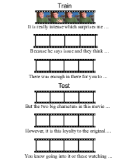
(d)

Figure 1: Input patterns of different modality inference problems. Here visual modality is the victim modality that may be missing randomly. (a) modalities are both complete in train and test set; (b) modalities are both complete in the train set but the victim modality is completely missing in the test set; (c) victim modality is missing randomly in the train set but completely missing in the test set; (d) modalities are missing with the same probability in train and test set.

In other words, data from each modality are more probable to be missing at random (Fig.1c and 1d) than completely present or missing (Fig.1a and 1b) (Pham et al., 2019; Tang et al., 2021; Zhao et al., 2021). Based on the complete input modality setting, a family of popular routines regarding the missing-modality inference is to design intricate generative modules attached to the main network and train the model under full supervision with complete modality data. By minimizing a customized reconstruction loss, the data restoration (a.k.a. missing data imputation Van Buuren (2018)) capability of the generative modules is enhanced (Pham et al., 2019; Wang et al., 2020; Tang et al., 2021) so that the model can be tested in the missing situations (Fig. 1b). However, we notice that (i) if modality-complete data in the training set is scarce, a severe overfitting issue may occur, especially when the generative model is large Robb et al. (2020); Schick and Schütze (2021); Ojha et al. (2021); (ii) global attention-based (i.e., attention over the whole sequence) imputation may bring unexpected noise since true correspondence mainly exists between temporally adjacent parallel signals Sakoe and Chiba (1978). Ma et al. (2021) proposed to leverage unit-length sequential representation to represent the missing modality from the seen complete modality from the input for training. Nevertheless, such kinds of methods inevitably overlook the temporal correlation between modality sequences and only acquire fair performance on the downstream tasks.

To mitigate these issues, in this paper we present MM-Align, a novel framework for fast and effective multimodal learning on randomly missing multimodal sequences. The core idea behind the framework is to imitate some indirect but informative clues for the paired modality sequences instead of learning to restore the missing modality directly. The framework consists of three essential functional units: 1) a backbone network that handles the main task; 2) an alignment matrix solver based on the optimal transport algorithm to produce context-window style solutions only part of whose values are non-zero and an associated meta-learner to imitate the dynamics and perform imputation in the modality-invariant hidden spaces; 3) a denoising training algorithm that optimizes and coalesces the backbone network and the learner so that they can work robustly on the main task in missing-modality scenarios. To empirically study the advantages of our models over current imputation approaches, we test on two settings of the random missing conditions, as shown in Fig. 1c and Fig. 1d, for all possible modality pair combinations. To the best of our knowledge, it is the first work that applies optimal transport and denoising training to the problem of inference on missing modality sequences. In a nutshell, the contribution of this work is threefold:

• We propose a novel framework to facilitate the missing modality sequence inference task, where we devise an alignment dynamics learning module based on the theory of optimal transport and a denoising training algorithm to coalesce it into the main network.

• We design a loss function that enables a context-window style solution for the dynamics solver.

• We conduct comprehensive experiments on three publicly available datasets from two multimodal tasks. Results and analysis show that our method leads to a faster and more accurate inference of missing modalities.

2 Related Work

2.1 Multimodal Learning

Multimodal learning has raised prevalent concentration as it offers a more comprehensive view of the world for the task that researchers intend to model Atrey et al. (2010); Lahat et al. (2015); Sharma and Giannakos (2020). The most fundamental technique in multimodal learning is multimodal fusion Atrey et al. (2010), which attempts to extract and integrate task-related information from the input modalities into a condensed representative feature vector. Conventional multimodal fusion methods encompass cross-modality attention Tsai et al. (2018, 2019); Han et al. (2021a), matrix algebra based method Zadeh et al. (2017); Liu et al. (2018); Liang et al. (2019) and invariant space regularization Colombo et al. (2021); Han et al. (2021b). While most of these methods focus on complete modality input, many take into account the missing modality inference situations Pham et al. (2019); Wang et al. (2020); Ma et al. (2021) as well, which usually incorporate a generative network to impute the missing representations by minimizing the reconstruction loss. However, the formulation under missing patterns remains underexplored, and that is what we dedicate to handling in this paper.

2.2 Meta Learning

Meta-learning, or learning to learn, is a hot research topic that focuses on how to generalize the learning approach from a limited number of visible tasks to broader task types. Early efforts to tackle this problem are based on comparison, such as relation networks Sung et al. (2018) and prototype-based methods Snell et al. (2017); Qi et al. (2018); Lifchitz et al. (2019). Other achievements reformulate this problem as transfer learning Sun et al. (2019) and multi-task learning Pentina et al. (2015); Tian et al. (2020), which devote to seeking an effective transformation from previous knowledge that can be adapted to new unseen data, and further fine-tune the model on the handcrafted hard tasks. In our framework, we treat the alignment matrices as the training target for the meta-learner. Combined with a self-adaptive denoising training algorithm, the meta-learner can significantly enhance the predictions’ accuracy in the missing modality inference problem.

3 Method

3.1 Problem Definition

Given a multimodal dataset $\mathcal{D}=\{\mathcal{D}^{train},\mathcal{D}^{val},\mathcal{D}^{test}\}$, where $\mathcal{D}^{train},\mathcal{D}^{val},\mathcal{D}^{test}$ are the training, validation and test set, respectively. In the training set $\mathcal{D}^{train}=\{(x_{i}^{m_{1}},x_{i}^{m_{2}},y_{i})_{i=1}^{n}\}$, where $x_{i}^{m_{k}}=\{x_{1,1}^{m_{k}},...,x_{i,t}^{m_{k}}\}$ are input modality sequences and $m_{1},m_{2}$ denote the two modality types, some modality inputs are missing with probability $p^{\prime}$. Following Ma et al. (2021), we assume that modality $m_{1}$ is complete and the random missing only happens on modality $m_{2}$, which we call the victim modality. Consequently, we can divide the training set into the complete and missing splits, denoted as $\mathcal{D}^{train}_{c}=\{(x_{i}^{m_{1}},x_{i}^{m_{2}},y_{i})_{i=1}^{n_{c}}\}$ and $\mathcal{D}^{train}_{m}=\{(x_{i}^{m1},y_{i})_{i=n_{c}+1}^{n}\}$, where $|\mathcal{D}^{train}_{m}|/|\mathcal{D}^{train}|=p^{\prime}$. For the validation and test set, we consider two settings: a) the victim modality is missing completely (Fig. 1c), denoted as “setting A” in the experiment section; b) the victim modality is missing with the same probability $p^{\prime}$ (Fig. 1d), denoted as “Setting B”, in line with Ma et al. (2021). We consider two multimodal tasks: sentiment analysis and emotion recognition, in which the label $y_{i}$ represents the sentiment value (polarity as positive/negative and value as strength) and emotion category, respectively.

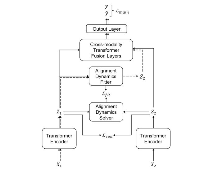
Figure 2: Overall architecture of our framework. Solid lines are the forward paths when training on the modality-complete split and dashed lines are the forward paths when training and testing on the split with missing modality.

3.2 Overview

Our framework encompasses a backbone network (green), an alignment dynamics learner (ADL, blue), and a denoising training algorithm to optimize both the learner and backbone network concurrently. We highlight the ADL which serves as the core functional unit in the framework. Motivated by the idea of meta-learning, we seek to generate substitution representations for the missing modality through an indirect imputation clue, i.e., alignment matrices, instead of learning to restore the missing modality by minimizing the reconstruction losses. To this end, the ADL incorporates an alignment matrix solver based on the theory of optimal transport Villani (2009), a non-parametric method to capture alignment dynamics between time series Peyré et al. (2019); Chi et al. (2021), as well as an auxiliary neural network to fit and generate meaningful representations as illustrated in section 3.4.

3.3 Architecture

Backbone Network

The overall architecture of our framework is depicted in Fig. 2. We harness MulT Tsai et al. (2019), a fusion network derived from Transformer Vaswani et al. (2017) as the backbone structure since we find a number of its variants in preceding works acquire promising outcomes in multimodal Wang et al. (2020); Han et al. (2021a); Tang et al. (2021). MulT has two essential components: the unimodal self-attention encoder and bimodal cross-attention encoder. Given modality sequences $x^{m_{1}},x^{m_{2}}$ (for unimodal self-attention we have $m_{1}=m_{2}$) as model’s inputs, after padding a special token $x_{0}^{m_{1}}=x_{0}^{m_{2}}=$[CLS] to their individual heads, a single transformer layer Vaswani et al. (2017) encodes a sequence through a multi-head attention (MATT) and feed-forward network (FFN) as follows:

$$Q=x^{m_{1}} W_{Q},K=x^{m_{2}}W_{K},V=x^{m_{2}}W_{V}$$ (1)

$$\hat{Z}^{21} =\mathrm{MATT}(Q,K,V)+x^{m_{1}}$$ (2)

$$Z^{21} =\mathrm{FFN}(\hat{Z}^{21})+\mathrm{LN}(\hat{Z}^{21})$$ (3)

where LN is layer normalization. In our experiments, we leverage this backbone structure for both input modality encoding and multimodal fusion.

Output Layer

We extract the head embeddings $z^{12}_{0},z^{21}_{0}$ from the output of the fusion network as features for regression. The regression network is a two-layer feed-forward network:

$$\hat{y}=W_{2}(\textrm{tanh}(W_{1}[z_{0}^{12},z_{0}^{21}]+b_{1})+b_{2}$$ (4)

where $[\boldsymbol{\cdot},\boldsymbol{\cdot},\cdots]$ is the concatenation operation. The mean squared error (MSE) is adopted as the loss function for the regression task:

$$\mathcal{L}_{main}=\mathrm{MSE}(\hat{y},y)$$ (5)

3.4 Alignment Dynamics Learner (ADL)

The learner has two functional modules, named as alignment dynamics solver and fitter, as shown in Fig. 2. It also runs in two functional modes, namely learning and decoding. ADL works in learning mode when the model is trained on the complete data (marked by the solid lines in Fig. 2). The decoding mode is triggered when one of the modalities is missing, which happens in the training time on the missing splits and the entire test time (marked by the dashed lines in Fig. 2).

Learning Mode

In the learning mode, the solver calculates an alignment matrix which provides the information about temporal correlations between the two modality sequences. Similar to the previous works Peyré et al. (2019); Chi et al. (2021), this problem can be formulated as an optimal transport (OT) task:

$$\min_{A}\sum_{i,j}A_{ij}M_{ij}$$ (6)

where $A$ is the transportation plan that implies the alignment information Peyré et al. (2019) and $M$ is the cost matrix. The subscript $ij$ represents the component from the $i$th timestamp in the source modality to the $j$ th timestamp in the target modality. Different from Peyré et al. (2019) and Chi et al. (2021) which allow alignment between any two positions of the two sequences, we believe that in parallel time series, the temporal correlation mainly exists between signals inside a time-specific “window” (i.e., $|j-i|\leq W$, where $W$ is the window size) Sakoe and Chiba (1978). Additionally, the cost function should be negatively correlated to the similarity (distance), as one of the problem settings in the original OT problem. To realize these basic motivations, we borrowed the concept of barrier function Nesterov et al. (2018) and define the cost function for our optimal transport problem as:

$$M_{ij}=\begin{cases}1-\cos{(z_{i}^{1},z_{j}^{2})},&|i-j|\leq K\\ \infty,&|i-j|>K\end{cases}$$ (7)

where $z_{i}^{m}$ is the representation of modality $m$ at timestamp $i$ and $cos(\cdot,\cdot)$ is the cosine value of two vectors. We will show that such a type of transportation cost function ensures a context-window style alignment solution and also provide a proof in appendix C. To solve Eq. (6), a common practice is to add an entropic regularization term:

$$\min_{A}\sum_{i,j}A_{ij}M_{ij}-\mu A_{ij}\log A_{ij}$$ (8)

The unique solution $A^{*}$ can be calculated through Sinkhorn’s algorithm Peyré et al. (2019):

$$A^{*}=\mathrm{diag}(\mathbf{u})K\mathrm{diag}(\mathbf{v}),K=\exp{(M/\mu)}$$ (9)

The vector $\mathbf{u}$ and $\mathbf{v}$ are obtained through the following iteration until convergence:

$$\mathbf{v}^{t=0} =\mathbf{1}_{m}$$ (10)

$$\mathbf{u}^{t+1} =\frac{\mathbf{1}_{n}}{K\mathbf{v}^{t}},\quad\mathbf{v}^{t+1}=\frac{\mathbf{1}_{n}}{K\mathbf{u}^{t+1}}$$ (11)

After quantifying the temporal correlation into alignment matrices, we enforce the learner to fit those matrices so that it can automatically approximate the matrices from the non-victim modality in the decoding mode. Specifically, a prediction network composed of a gated recurrent unit Chung et al. (2014) and a linear projection layer takes the shared representations of the complete modality as input and outputs the prediction value for entries:

$$\hat{T}=\mathrm{softmax}(\mathrm{Linear}(\mathrm{GRU}(Z^{1};\psi_{r});\psi_{p}))$$ (12)

where $\psi=\{\psi_{r},\psi_{t}\}$ is the collection of parameters in the prediction network. $\hat{T}=\{\hat{t}_{1},\hat{t}_{2},...,\hat{t}_{l}\}\in\mathbb{R}^{l\times(2W+1)}$ are the predictions for $A^{*}$ and $\hat{t}_{i}\in\mathbb{R}^{2W+1}$ is the prediction for the alignment matrix segment $A^{*}_{i,i-W:i+W}$, i.e., the alignment components which span within the radius of $W$ centered at current timestamp $i$. We reckon the mean squared error (MSE) between “truths" generated from the solver and predictions to calculate the fitting loss:

$$\mathcal{L}_{fit}=\frac{1}{(2W+1)l}\sqrt{\sum_{i}\sum_{j=i-W}^{i+W}(A^{*}_{ij}-\hat{T}_{ij})^{2}}$$ (13)

where the summation is over the entries within context windows and we define $A^{*}_{ij}=0$ if $j\leq 0$ or $j>l$ for better readability.

Decoding Mode

In this mode, the learner behaves like a decoder that strives to generate meaningful substitution to the missing modality sequences. The learner first decodes an alignment matrix $\hat{A}$ via the fitting network whose parameters are frozen during this stage. Afterward, the imputation of the missing modality at position $j$ can be obtained through the linear combination of alignment matrices and visible sequences:

$$\hat{z}_{j}^{2}=\sum_{i=j-W}^{j+W}\hat{A}_{ij}z_{i}^{1}$$ (14)

We concatenate all these vectors to construct the imputation for the missing modality $\hat{Z}^{2}$ in the shared space:

$$\hat{Z^{2}}=[\hat{z}_{0}^{2},\hat{z}_{1}^{2},\hat{z}_{2}^{2},...,\hat{z}_{l}^{2}]$$ (15)

where $\hat{z}_{0}^{2}$ is reassigned by the initial embedding of the [CLS] token. The imputation results together with the complete modality sequences are then fed into the fusion network (Eq. (1) ~(3)) to continue the subsequent procedure.

Input: $\mathcal{D}^{train}=\{\mathcal{D}^{train}_{c},\mathcal{D}^{train}_{m}\}$, learning rate $\eta_{fit},\eta_{main}$, parameters of the backbone network $\theta=\{\theta_{enc},\theta_{fu},\theta_{out}\}$ and the alignment dynamics learner $\psi=\{\psi_{d}\}$, batch size $n_{b}$, $\lambda$

// Warm-up Stage

1 for each warm-up epoch do

2       for each $\mathcal{B}=\{\cup_{i=1}^{n_{b}}(x^{m_{1}}_{i},x^{m_{2}}_{i},y_{i})\}\subset\mathcal{D}^{train}_{c}$ do

3             Compute $\mathcal{L}_{main},\mathcal{L}_{con}$ by Eq. (1)~(5), (16), (17)

4             $\theta\leftarrow\theta-\eta_{main}\nabla_{\theta}(\mathcal{L}_{main}+\lambda\mathcal{L}_{cons})$

5       end for

6      

7 end for

8for each training epoch do

       // Train on the complete split

9       for each $\mathcal{B}=\{\cup_{i=1}^{n_{b}}(x^{m_{1}}_{i},x^{m_{2}}_{i},y_{i})\}\subset\mathcal{D}^{train}_{c}$ do

10             Compute $A^{*}$ by Sinkhorn algorithm according to Eq. (7)~(11)

11             Compute $\mathcal{L}_{fit}$ according to (13);

             // Tune the dynamics learner

12             $\psi\leftarrow\psi-\eta_{fit}\nabla_{\psi}\mathcal{L}_{fit}$

13             Compute $\mathcal{L}_{main},\mathcal{L}_{con}$ according to Eq. (1)~(5), (16), (17)

             // Tune the backbone network

14             $\theta\leftarrow\theta-\eta_{main}\nabla_{\theta}(\mathcal{L}_{main}+\lambda\mathcal{L}_{cons})$

15       end for

      // Train on the missing split

16       for each $\mathcal{B}=\{\cup_{i=1}^{n_{b}}(x^{m_{1}}_{i},y_{i})\}\subset\mathcal{D}^{train}_{m}$ do

17             Impute the representation sequences of the missing modality $\hat{Z}_{i}^{2}$ by Eq. (14) (15) and then $\mathcal{L}_{main}$ by Eq. (1)~(5), (16), (17) $\theta\leftarrow\theta-\eta_{main}\nabla_{\theta}\mathcal{L}_{main}$

18       end for

19      

20 end for

Algorithm 1 Denoising Training

3.5 Denoising Training

Inspired by previous work in data imputation Kyono et al. (2021), we design a denoising training algorithm to promote prediction accuracy and imputation quality concurrently, as shown in Alg. 1. In the beginning, we warm up the model on the complete split of the training set. We utilize two transformer encoders to project input modality sequences $x^{m_{1}}$ and $x^{m_{2}}$ into a shared feature space, denoted as $Z^{1}$ and $Z^{2}$. Following Han et al. (2021b), we apply a contrastive loss Chen et al. (2020) as the regularization term to force a similar distribution of the generated vectors $Z^{1}$ and $Z^{2}$:

$$\mathcal{L}_{con}=-\frac{1}{N_{b}}\sum_{i}\log\frac{\phi(Z^{1}_{i},Z_{i}^{2})}{\sum_{j}\phi(Z_{i}^{1},Z_{j}^{2})}$$ (16)

where the summation is over the whole batch of size $N_{b}$ and $\phi$ is a score function with an annealing temperature $\tau$ as the hyperparameter:

$$\phi(s,t)=\exp{(s^{T}t/\tau)}$$ (17)

Next, the denoising training loop proceeds to couple the ADL and backbone network. In a single loop, we first train the alignment dynamics learner (line 9~11), then we train the backbone network on the complete split (line 12~13) and missing split (line 15~17). Since the learner training process uses the modality-complete split, and we found in experiments (section 4.4) that model’s performance stays nearly constant if the tuning for the learner and the main network occurs concurrently on every batch, we merge them into a single loop (line 8~14) to reduce the redundant batch iteration.

4 Experiments

4.1 Datasets

We utilize CMU-MOSI Zadeh et al. (2016) and CMU-MOSEI Zadeh et al. (2018) for sentiment prediction, and MELD Poria et al. (2019) for emotion recognition, to create our evaluation benchmarks. The statistics of these datasets and preprocessing steps can be found in appendix A. All these datasets consist of three parallel modality sequences—text (t), visual (v) and acoustic (a). In a single run, we extract a pair of modalities and select one of them as the victim modality which we then randomly remove $p^{\prime}=1-p$ of all its sequences. Here $p$ is the surviving rate for the convenience of description. We preprocess test sets as Fig. 1c (remove all victim modality samples) in setting A and Fig. 1d (randomly remove $p^{\prime}$ of victim modality samples) in setting B. Setting B inherits from Ma et al. (2021) while the newly added setting A is considered as a complementary test case of more severe missing situations, which can compare the efficacy of pure imputation methods and enrich the connotation of robust inference. We run experiments with two randomly picking $p\in\{10\%,50\%\}$— dissimilar to Ma et al. (2021), we enlarge the gap between two $p$ values to strengthen the distinction between these settings.

4.2 Baselines and Evaluation Metrics

We compare our models with the following relevant and strong baselines:

• Supervised-Single trains and tests the backbone network on a single complete modality, which can be regarded as the lower bound (LB) for all the baselines.

• Supervised-Double trains and tests the backbone network on a pair of complete modalities, which can be regarded as the upper bound (UB).

• MFM Tsai et al. (2018) learns modality-specific generative factors that can be produced from other modalities at training time and imputes the missing modality based on these factors at test time.

• SMIL Ma et al. (2021) imputes the sequential representation of the missing modality by linearly adding clustered center vectors with weights from learned Gaussian distribution.

• Modal-Trans Wang et al. (2020); Tang et al. (2021) builds a cyclic sequence-to-sequence model and learns bidirectional reconstruction.

The characteristics of all these models are listed for comparison in Table 1. Previous work relies on either a Gaussian generative or sequence-to-sequence formulation to reconstruct the victim modality or its sequential representations, while our model adopts none of these architectures. We run our models under 5 different splits and report the average performance. The training details can be found in appendix B.

We compare these models on the following metrics: for the sentiment prediction task, we employ the mean absolute error (MAE) which quantifies how far the prediction value deviates from the ground truth, and the binary classification accuracy (Acc-2) that counts the proportion of samples correctly classified into positive/negative categories; for emotion recognition task we compare the average F1 score over seven emotional classes.

Model	Generative Gaussian	Recon	Seq2Seq
MFM	✗	✓	✓
SMIL	✓	✓	✗
Modal-Trans	✗	✓	✓
MM-Align (Ours)	✗	✗	✗

Table 1: Model characteristics.

Method	T $\rightarrow$ V				V$\rightarrow$A				A$\rightarrow$T
	Setting A		Setting B		Setting A		Setting B		Setting A		Setting B
	MAE$\downarrow$	Acc-2$\uparrow$	MAE$\downarrow$	Acc-2$\uparrow$	MAE$\downarrow$	Acc-2$\uparrow$	MAE$\downarrow$	Acc-2$\uparrow$	MAE$\downarrow$	Acc-2$\uparrow$	MAE$\downarrow$	Acc-2$\uparrow$
LB	1.242	68.6	1.242	68.6	1.442	46.4	1.442	46.4	1.440	42.2	1.440	42.2
UB	1.019	77.7	1.019	77.7	1.413	57.8	1.413	57.8	1.081	75.8	1.081	75.8
MFM	1.103	71.0	1.093	73.2	1.456	43.5	1.452	43.9	1.477	42.2	1.454	42.2
SMIL	1.073	74.2	1.052	75.3	1.442	45.9	1.438	46.5	1.447	43.3	1.439	45.4
Modal-Trans	1.052	75.5	1.041	75.8	1.428	49.4	1.425	49.7	1.435	48.7	1.432	48.9
MM-Align	1.028♮	76.9♮	1.027	77.0	1.416♮	52.0♮	1.411♮	53.1♮	1.426	51.5♮	1.414♮	52.0♮
	V $\rightarrow$ T				A$\rightarrow$V				T$\rightarrow$A
	Setting A		Setting B		Setting A		Setting B		Setting A		Setting B
	MAE$\downarrow$	Acc-2$\uparrow$	MAE$\downarrow$	Acc-2$\uparrow$	MAE$\downarrow$	Acc-2$\uparrow$	MAE$\downarrow$	Acc-2$\uparrow$	MAE$\downarrow$	Acc-2$\uparrow$	MAE$\downarrow$	Acc-2$\uparrow$
LB	1.442	46.3	1.442	46.3	1.440	42.2	1.440	42.2	1.242	68.6	1.242	68.6
UB	1.019	77.7	1.019	77.7	1.413	57.8	1.413	57.8	1.081	75.8	1.081	75.8
MFM	1.479	42.2	1.429	51.9	1.454	42.2	1.455	42.2	1.078	72.9	1.082	73.7
SMIL	1.448	44.2	1.447	43.3	1.442	45.9	1.438	47.3	1.060	75.5	1.089	74.9
Modal-Trans	1.429	50.3	1.420	53.1	1.439	47.4	1.442	48.3	1.052	75.2	1.073	74.3
MM-Align	1.415♮	52.7♮	1.410	53.4	1.427♮	49.9♮	1.426♮	50.7♮	1.028♮	76.7♮	1.032♮	76.6♮

Table 2: Results on the CMU-MOSI dataset ($p=10$). The reported results are the average of five runs using the same set of hyperparameters and different random seeds. “A $\to$ B” means the imputation from the complete modality A to the missing modality B at the test time. $\natural$: results of our model are significantly better than the highest baselines with p-value $<$ 0.05 based on the paired t-test.

Method	T $\rightarrow$ V				V$\rightarrow$A				A$\rightarrow$T
	Setting A		Setting B		Setting A		Setting B		Setting A		Setting B
	MAE$\downarrow$	Acc-2$\uparrow$	MAE$\downarrow$	Acc-2$\uparrow$	MAE$\downarrow$	Acc-2$\uparrow$	MAE$\downarrow$	Acc-2$\uparrow$	MAE$\downarrow$	Acc-2$\uparrow$	MAE$\downarrow$	Acc-2$\uparrow$
LB	0.687	77.4	0.687	77.4	0.836	61.3	0.836	61.3	0.851	62.9	0.851	62.9
UB	0.615	81.3	0.615	81.3	0.707	79.5	0.707	79.5	0.613	80.9	0.613	80.9
MFM	0.658	79.2	0.645	80.0	0.827	61.5	0.818	61.9	0.836	64.3	0.830	63.6
SMIL	0.680	78.3	0.648	78.5	0.819	64.3	0.816	63.6	0.840	62.9	0.839	63.0
Modal-Trans	0.645	79.6	0.647	79.6	0.818	64.7	0.815	65.4	0.827	64.9	0.823	65.6
MM-Align	0.637♮	80.8♮	0.638♮	81.1♮	0.811♮	65.9♮	0.813	66.2♮	0.824	65.3	0.817	66.3
	V $\rightarrow$ T				A$\rightarrow$V				T$\rightarrow$A
	Setting A		Setting B		Setting A		Setting B		Setting A		Setting B
	MAE$\downarrow$	Acc-2$\uparrow$	MAE$\downarrow$	Acc-2$\uparrow$	MAE$\downarrow$	Acc-2$\uparrow$	MAE$\downarrow$	Acc-2$\uparrow$	MAE$\downarrow$	Acc-2$\uparrow$	MAE$\downarrow$	Acc-2$\uparrow$
LB	0.836	61.3	0.836	61.3	0.851	62.9	0.851	62.9	0.687	77.4	0.687	77.4
UB	0.615	81.3	0.615	81.3	0.707	79.5	0.707	79.5	0.613	80.9	0.613	80.9
MFM	0.821	62.0	0.817	61.7	0.842	62.7	0.828	63.9	0.658	79.1	0.645	79.7
SMIL	0.820	63.1	0.816	63.5	0.838	63.2	0.842	62.4	0.684	78.5	0.684	77.4
Modal-Trans	0.817	65.1	0.814	65.7	0.832	64.6	0.823	65.1	0.643	79.9	0.645	79.4
MM-Align	0.811♮	66.2♮	0.806♮	66.9♮	0.822♮	65.4♮	0.818	65.7	0.635♮	81.0♮	0.637♮	80.9♮

Table 3: Results on the CMU-MOSEI dataset ($p=10)$. Notations share the same meaning as the last table.

Method	A	B	A	B	A	B
	T $\rightarrow$ V		V$\rightarrow$A		A$\rightarrow$T
LB	54.0	54.0	31.3	31.3	31.3	31.3
UB	55.8	55.8	32.1	32.1	55.9	55.9
MFM	54.0	53.9	31.3	31.3	31.3	43.1
SMIL	54.4	54.2	31.3	31.3	31.3	43.5
Modal-Trans	55.0	54.8	31.3	31.4	31.5	44.4
MM-Align	55.7	55.7	31.9	31.9♮	31.5	45.5
	V $\rightarrow$ T		A $\rightarrow$V		T $\rightarrow$A
LB	31.3	31.3	31.3	31.3	54.0	54.0
UB	55.8	55.8	32.1	32.1	55.9	55.9
MFM	31.4	43.6	31.3	31.3	54.2	54.1
SMIL	31.4	43.9	31.3	31.3	54.5	54.2
Modal-Trans	31.6	44.2	31.3	31.3	55.0	54.8
MM-Align	32.3	45.4	31.3	32.0	55.6	55.7

Table 4: Results on MELD ($p=50\%$). Notations share the same meaning as the last table.

4.3 Results

Due to the particularities of three datasets, We report the results of the smallest $p$ values when most of these baselines yield $1\%$ higher results than the lower bound in Table 2, 3 and 4. From them we mainly have the following observations:

First, Compared with lower bounds, in setting A where models are tested with only the non-victim modality, our method gains 6.6%~9.3%, 2.4%~4.9% accuracy increment on the CMU-MOSI and CMU-MOSEI dataset and 0.6%~1.7% F1 increment on the MELD dataset (except A$\to$V and A$\to$T). Besides, MM-Align significantly outperforms all the baselines in most settings. These facts indicate that leveraging the local alignment information as indirect clues facilitates to performing robust inference on missing modalities.

Second, model performance varies greatly especially when the non-victim modality alters. It has been pointed out that three modalities do not play an equal role in multimodal tasks Tsai et al. (2019). Among them, the text is usually the predominant modality that contributes majorly to accuracy, while visual and acoustic have weaker effects on the model’s performance. From the results, it is apparent that if the source modality is predominant, the model’s performance gets closer to or even surpasses the upper bound, which reveals that the predominant modality can also offer richer clues to facilitate the dynamics learning process than other modalities.

Third, when moving from setting A to setting B by adding parallel sequences of the non-victim modality in the test set, results incline to be constant in most settings. Intuitively, performance should become better if more parallel data are provided. However, as most of these models are unified and must learn to couple the restoration/imputation module and backbone network, the classifier inevitably falls into the dilemma that it should adapt more to the true parallel sequences or the mixed sequences since both are included patterns in a training epoch. Hence sometimes setting B would not perform evidently better than setting A. Particularly, we find that when Modal-Trans encounters overfitting, MM-Align can alleviate this trend, such as T$\to$A in all three datasets.

Additionally, MM-Align acquires a 3~4$\times$ speed-up in training. We record the time consumption and provide a detailed analysis in appendix D and E.

Settings	T $\rightarrow$ V		V$\rightarrow$A		A$\rightarrow$T
	MAE$\downarrow$	Acc-2$\uparrow$	MAE$\downarrow$	Acc-2$\uparrow$	MAE$\downarrow$	Acc-2$\uparrow$
MM-Align	1.028	76.9	1.416	52.0	1.426	51.5
w/o $\mathcal{L}_{con}$	1.037	76.7	1.422	51.8	1.432	49.5
w/o $\mathcal{L}_{fit}$	1.085	72.2	1.437	47.3	1.448	44.6
w/o SI	1.033	76.6	1.425	51.9	1.419	51.8

Table 5: Results of ablation experiments on CMU-MOSI dataset.

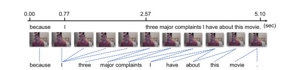
Figure 3: An example from CMU-MOSI dataset. The text below the time axis is aligned to the starting time of its pronunciation. The pictures are the central frame of each cluster that lasts the same time interval. The dashed lines connect each word with the frames of its appearance in the video.

4.4 Ablation Study

We run our model under the following ablative settings on three randomly chosen modality pairs from the CMU-MOSI dataset in setting A: 1) removing the contrastive loss which serves as the invariant space regularizer; 2) removing the fitting loss so that the ADL only generates a random alignment matrix when running in the inference mode; 3) separating the single iteration (SI) over the complete split that concurrently optimizes the fitter and backbone network in Alg. 1 into two independent loops. The results of these experiments are displayed in Table 5. We witness a performance drop after removing the contrastive loss, and the drop is higher if we disable the ADL, which implies the benefits from the alignment dynamics-based generalization process on the modality-invariant hidden space. Finally, merging two optimization steps will not cause performance degradation. Therefore it is more time-efficient to design the denoising loop as Alg. 1 to prevent an extra dataset iteration.

5 Analysis

Impact of the Window Size

To further explore the impact of window size, we run our models by increasing window size from 4 to 256 which exceeds the lengths of all sentences so that all timestamps are enclosed by the window. The variation of MAE and F1 in this process is depicted in Fig. 4. There is a dropping trend (MAE increment or F1 decrement) towards both sides of the optimal size. We argue that it is because when the window expands, it is more probable for the newly included frame to add noise rather than provide valuable alignment information. In the beginning, the marginal benefit is huge so the performance almost keeps climbing. The optimal size is reached when the marginal benefit decreases to zero.

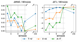
Figure 4: Performance variation under different window sizes. The optimal sizes for the three pairs are 9, 10, 10.

To explain this claim, we randomly select a raw example from the CMU-MOSI dataset. As shown in Fig. 3, the textual expression does not advance in a uniform speed. From the second to the third word 1.80 seconds elapses, while the last eight words are covered in only 2.53 seconds. Intuitively we can assume all the frames in the video that span across the pronunciation of a word are causally correlated with that word so that the representation mappings from the word to these frames are necessary and can benefit the downstream tasks. For example, for the word “I” present at $t=1$ in text, it can benefit the timestamps until at least $t=5$ in the visual modality. Note that we may overlook some potential advantages that could not be easily justified in this way and possess different effect scope, but we deem that those advantages would like-wisely disappear as the window size keeps growing.

6 Conclusion

In this paper, we propose MM-Align, a fast and efficient framework for the problem of missing modality inference. It applies the theory of optimal transport to learn the alignment dynamics between temporal modality sequences for the inference in the case of missing modality sequences. Experiments on three datasets of demonstrate that MM-Align can achieve much better performance and thus reveal the higher robustness of our method. We hope that our work can inspire other research works in this field.

Limitations

Although our model has successfully tackled the two missing patterns, it may still fail in more complicated cases. For example, if missing happens randomly in terms of frames (some timestamps within a unimodal clip) instead of instances (the entire unimodal clip), then our proposed approach could not be directly used to deal with the problem, since we need at least several instances of complete parallel data to learn how to map from one modality sequences to the other. However, we believe these types of problems can still be properly solved by adding some mathematical tools like interpolation, etc. We will consider this idea as the direction of our future work.

Besides, the generalization capability of our framework on other multimodal tasks is not clear. But at least we know the feasibility highly depends on the types of target tasks, especially the input formats—they have to be parallel sequences so that temporal alignment information between these sequences can be utilized. The missing patterns should be similar to what we described in section 2, as we discussed in the first paragraph.

Appendix A Dataset Statistics and Preprocessing

The statistics of the two datasets are listed in Table 6. MELD is originally a dialogue emotion detection dataset, where each dialogue contains many sentences. Since we want to make it compatible with tested models, we extract all sentences and remove those that lack at least one modality (text, visual, acoustic). Following previous work, for MOSI and MOSEI we use COVAREP Degottex et al. (2014) and P2FA Yuan et al. (2008) to respectively extract visual and acoustic features. For MELD, we use ResNet-101 He et al. (2016) and Wave2Vec 2.0 Baevski et al. (2020) to extract visual and acoustic features.

Dataset	Train	Dev	Test	Total
CMU-MOSI	1284	229	686	2299
CMU-MOSEI	16326	1871	4859	22856
MELD	9988	1108	2610	13706

Table 6: Statistics of three datasets we use for experiments.

Appendix B Hyperparameter Search

All these models are trained on a single RTX A6000 GPU. We use Glove Pennington et al. (2014) 300d to initialize the embedding of all the tokens. We perform a grid search for part of the hyperparameters as Table 7.

HP-name	CMU-MOSI	CMU-MOSEI	MELD
$\eta_{main}$	1e-3,2e-3	1e-4	1e-3,1e-4
$\eta_{fit}$	1e-4,5e-4,1e-3	2e-5,1e-4	5e-4,5e-5
attn_dim	32,40	32,40	32,64
num_head	4,8	4,8	4,8
$n_{b}$	32	32	32
warm-up	1,2	1,2	1
patience	10	5	5
$\lambda$	0.05,0.1	0.05,0.1	0.05,0.1
$K$	4,5,8,9,10	4,5,6,7,8	3,4,5,8

Table 7: The hyperparameter search for three datasets

Appendix C OT Solution

C.1 Visualization of Solutions

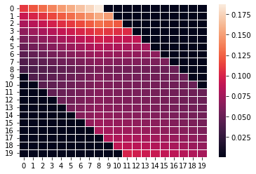
Figure 5: The average absolute entry values of the produced alignment matrices (window size=8).

To verify our statement in Section 3.4 that the learned dynamics matrices are in the window style, we calculate and visualize the mean absolute values for each entry. Due to various sentence lengths, the values are averaged over all matrices whose corresponding input sequences’ lengths are no smaller than 20. We visualize the heat map of the average entry values in Fig. 5. It can be clearly viewed that the values outside the window stay nearly 0 (black squares), implying that they are always close to 0.

C.2 Proof of solution pattern

We formalize the window style solution in mathematical language.

Theorem 1.

Given the optimal transport formulation as Eq. (6)~ (8). All the entries $a^{*}_{ij}$ that satisfy $|i-j|>W$ in the optimal transport plan $A^{*}$ are 0, where $W$ is the window size.

Proof.

We use the proof by contradiction. Assume there is an entry $A_{i^{\prime}j^{\prime}}$ in $A^{*}$ outside the window, i.e., $|i^{\prime}-j^{\prime}|>W$, and $A_{i^{\prime}j^{\prime}}>0$. Then we have the cost $C=\sum A^{*}_{ij}M_{ij}\geq A_{i^{\prime}j^{\prime}}\times M_{i^{\prime}j^{\prime}}\to\infty$. It is easy to find another path $i^{\prime}\to k_{1}\to k_{2}\to\cdots\to k_{n}\to j^{\prime}$, where $max(|i^{\prime}-k_{1}|,|k_{t}-k_{t-1}|,|j^{\prime}-k_{n}|)\leq W$. In this new transport plan $A^{\prime}$ simply we have $\sum A^{\prime}_{ij}M_{ij}<\infty$, which means $A^{*}$ is not the optimal transport plan and contradicts our basic assumption. Hence, by applying this kind of cost function we can obtain a window-style solution. ∎

Appendix D Complexity Analysis

We conduct a simple analysis of the computational complexity of MM-Align and Modal-Trans. We are concern about the stage that occupies the most time in one training epoch—training on the missing split when the ADL works in the decoding mode. Suppose the average sequence length, the embedding dimension, the window size are $l$, $d$ and $w$ (here $w$ stands for the value of $2W+1$ for simplicity), respectively. The complexity (number of multiplication operations) of the alignment dynamics fitter is the summation of the complexity from GRU and the linear projection layer:

$$O(c_{1}ld^{2})+O(c_{2}wld)\approx O(ld^{2})$$ (18)

The time spent on the alignment dynamics solver can be ignored since it is a non-parametric module so that no gradients are back-propagated through it and the number of iterations required for convergence is very little (about 5). The complexity of the transformer decoder is the summation of the complexity from encoder-decoder attention, encoder & decoder self-attention, and linear projections:

$$O(c_{1}l^{3}d)+O(c_{2}ld^{2})+O(c_{3}l^{2}d)\approx O(l^{3}d)>O(ld^{2})$$ (19)

The last inequality is an empirical conclusion, since in our experiments $l\approx 10$ while $d=32$ in most situations.

Particularly, the complexity of encoder-decoder attention can be calculated by the summation of $l$ times individual attention in the decoding procedure:

$$O(\sum_{i=1}^{l}(ild+ild))=O((1+l)l\times ld)\approx O(l^{3}d)$$ (20)

It should be highlighted that the computation only counts the number of multiplications into account. Since sequence-to-sequence decoding can not be paralleled, it takes more time to train.

Appendix E Inference Speed

As we mentioned before, the most competitive baseline, Modal-Trans, is a variant of the most advanced sequence-to-sequence model. Apart from the performance improvement, MM-Align also speeds up the training process. To show this, we run and calculate the average batch training time between MM-Align and Modal-Trans. As shown in Table 8, MM-Align achieves over 3$\times$ training acceleration over Modal-Trans but can produce sequential imputation of higher quality. We also provide an estimation for the computational complexity in the appendix.

Model	CMU-MOSI	CMU-MOSEI	MELD
Modal-Trans	0.811	1.270	0.954
MM-Align (window size=8)	0.278	0.340	0.312

Table 8: The average training time of the imputation module (seconds) per batch.

Appendix F Additional Results

In the main text, we present the results of the minimum $p$ in both settings. Here we also provide the results when tested in setting A for the two preservation in Table 9, 10 and 11.

Method	T $\rightarrow$ V				V$\rightarrow$A				A$\rightarrow$T
	10%		50%		10%		50%		10%		50%
	MAE$\downarrow$	Acc-2$\uparrow$	MAE$\downarrow$	Acc-2$\uparrow$	MAE$\downarrow$	Acc-2$\uparrow$	MAE$\downarrow$	Acc-2$\uparrow$	MAE$\downarrow$	Acc-2$\uparrow$	MAE$\downarrow$	Acc-2$\uparrow$
Supervised-Single (LB)	1.242	68.6	1.242	68.6	1.442	46.4	1.442	46.4	1.440	42.2	1.440	42.2
Supervised-Both (UB)	1.019	77.7	1.019	77.7	1.413	57.8	1.413	57.8	1.081	75.8	1.081	75.8
MFM	1.103	71.0	1.098	73.1	1.456	43.5	1.471	42.2	1.477	42.2	1.451	42.7
SMIL	1.073	74.2	1.060	75.0	1.442	45.9	1.471	42.7	1.447	43.3	1.473	45.3
Modal-Trans	1.052	75.5	1.031	75.9	1.428	49.4	1.417	51.1	1.435	48.7	1.415	53.7
MM-Align (Ours)	1.028	76.9	1.015	77.1	1.416	52.0	1.410	53.2	1.426	51.5	1.414	54.9
	V $\rightarrow$ T				A$\rightarrow$V				T$\rightarrow$A
	10%		50%		10%		50%		10%		50%
	MAE$\downarrow$	Acc-2$\uparrow$	MAE$\downarrow$	Acc-2$\uparrow$	MAE$\downarrow$	Acc-2$\uparrow$	MAE$\downarrow$	Acc-2$\uparrow$	MAE$\downarrow$	Acc-2$\uparrow$	MAE$\downarrow$	Acc-2$\uparrow$
Supervised-Single (LB)	1.442	46.4	1.442	46.4	1.440	42.2	1.440	42.2	1.242	68.6	1.242	68.6
Supervised-Both (UB)	1.019	77.7	1.019	77.7	1.413	57.8	1.413	57.8	1.081	75.8	1.081	75.8
MFM	1.446	45.5	1.429	48.3	1.454	42.2	1.467	42.2	1.078	72.9	1.083	73.3
SMIL	1.448	44.2	1.461	46.1	1.442	45.9	1.441	46.4	1.060	75.5	1.091	74.9
Modal-Trans	1.429	50.1	1.398	54.2	1.439	47.4	1.431	52.5	1.052	75.2	1.028	76.7
MM-Align (Ours)	1.415	52.7	1.399	55.4	1.427	49.9	1.413	56.6	1.028	76.7	1.025	76.7

Table 9: CMU-MOSI results in setting A (Fig. 1c), where $p=10\%$ and $50\%$.

Method	T $\rightarrow$ V				V$\rightarrow$A				A$\rightarrow$T
	10%		50%		10%		50%		10%		50%
	MAE$\downarrow$	Acc-2$\uparrow$	MAE$\downarrow$	Acc-2$\uparrow$	MAE$\downarrow$	Acc-2$\uparrow$	MAE$\downarrow$	Acc-2$\uparrow$	MAE$\downarrow$	Acc-2$\uparrow$	MAE$\downarrow$	Acc-2$\uparrow$
Supervised-Single (LB)	0.687	77.4	0.687	77.4	0.836	61.3	0.836	61.3	0.851	62.9	0.851	62.9
Supervised-Both (UB)	0.615	81.3	0.615	81.3	0.707	79.5	0.707	79.5	0.613	80.9	0.613	80.9
MFM	0.658	79.2	0.641	78.7	0.827	60.7	0.816	62.4	0.830	64.5	0.836	63.5
SMIL	0.680	78.3	0.654	78.5	0.819	64.3	0.815	64.6	0.840	62.9	0.835	63.5
Modal-Trans	0.645	79.6	0.641	79.5	0.818	64.7	0.814	64.7	0.827	64.9	0.820	64.7
MM-Align (Ours)	0.637	80.8	0.623	81.0	0.811	65.9	0.808	66.1	0.824	65.3	0.817	65.7
	V $\rightarrow$ T				A$\rightarrow$V				T$\rightarrow$A
	10%		50%		10%		50%		10%		50%
	MAE$\downarrow$	Acc-2$\uparrow$	MAE$\downarrow$	Acc-2$\uparrow$	MAE$\downarrow$	Acc-2$\uparrow$	MAE$\downarrow$	Acc-2$\uparrow$	MAE$\downarrow$	Acc-2$\uparrow$	MAE$\downarrow$	Acc-2$\uparrow$
Supervised-Single (LB)	0.836	61.3	0.836	61.3	0.851	62.9	0.851	62.9	0.687	77.4	0.687	77.4
Supervised-Both (UB)	0.615	81.3	0.615	81.3	0.707	79.5	0.707	79.5	0.613	80.9	0.613	80.9
MFM	0.821	62.0	0.820	64.5	0.842	62.7	0.835	62.4	0.658	79.1	0.659	78.9
SMIL	0.820	63.1	0.817	63.5	0.838	63.2	0.829	64.2	0.684	78.5	0.658	79.4
Modal-Trans	0.817	64.9	0.815	64.9	0.832	64.6	0.825	64.7	0.643	79.9	0.648	79.7
MM-Align (Ours)	0.812	65.2	0.807	66.9	0.822	65.4	0.819	66.0	0.635	81.0	0.626	80.9

Table 10: CMU-MOSEI results in Setting A ($p=10\%$ and $50\%$).

Method	10%	50%	10%	50%	10%	50%
	T $\rightarrow$ V		V$\rightarrow$A		A$\rightarrow$T
Supervised-Single (LB)	54.0	54.0	31.3	31.3	31.3	31.3
Supervised-Both (UB)	55.8	55.8	32.1	32.1	55.9	55.9
MFM	54.0	54.0	31.3	31.3	31.3	43.1
SMIL	54.1	54.4	31.3	31.3	31.3	43.5
Modal-Trans	54.2	55.0	31.3	31.4	31.5	44.4
MM-Align (Ours)	54.2	55.7	31.3	31.9	31.5	45.5
	V $\rightarrow$ T		A $\rightarrow$V		T $\rightarrow$A
Supervised-Single (LB)	31.3	31.3	31.3	31.3	54.0	54.0
Supervised-Both (UB)	55.8	55.8	32.1	32.1	55.9	55.9
MFM	31.4	43.6	31.3	31.3	54.2	54.1
SMIL	31.4	43.9	31.3	31.3	54.5	54.2
Modal-Trans	31.6	44.2	31.3	31.3	55.0	54.8
MM-Align (Ours)	32.3	45.4	31.3	32.0	55.6	55.7

Table 11: Results on MELD ($p=10\%$ and $50\%$) in setting A.

References

- Atrey et al. (2010) Pradeep K Atrey, M Anwar Hossain, Abdulmotaleb El Saddik, and Mohan S Kankanhalli. 2010. Multimodal fusion for multimedia analysis: a survey. Multimedia systems, 16(6):345–379.
- Baevski et al. (2020) Alexei Baevski, Yuhao Zhou, Abdelrahman Mohamed, and Michael Auli. 2020. wav2vec 2.0: A framework for self-supervised learning of speech representations. Advances in Neural Information Processing Systems, 33:12449–12460.
- Baltrušaitis et al. (2018) Tadas Baltrušaitis, Chaitanya Ahuja, and Louis-Philippe Morency. 2018. Multimodal machine learning: A survey and taxonomy. IEEE transactions on pattern analysis and machine intelligence, 41(2):423–443.
- Caesar et al. (2020) Holger Caesar, Varun Bankiti, Alex H Lang, Sourabh Vora, Venice Erin Liong, Qiang Xu, Anush Krishnan, Yu Pan, Giancarlo Baldan, and Oscar Beijbom. 2020. nuscenes: A multimodal dataset for autonomous driving. In Proceedings of the IEEE/CVF conference on computer vision and pattern recognition, pages 11621–11631.
- Chen et al. (2020) Ting Chen, Simon Kornblith, Mohammad Norouzi, and Geoffrey Hinton. 2020. A simple framework for contrastive learning of visual representations. In International conference on machine learning, pages 1597–1607. PMLR.
- Chi et al. (2021) Zewen Chi, Li Dong, Bo Zheng, Shaohan Huang, Xian-Ling Mao, He-Yan Huang, and Furu Wei. 2021. Improving pretrained cross-lingual language models via self-labeled word alignment. In Proceedings of the 59th Annual Meeting of the Association for Computational Linguistics and the 11th International Joint Conference on Natural Language Processing (Volume 1: Long Papers), pages 3418–3430.
- Chung et al. (2014) Junyoung Chung, Caglar Gulcehre, KyungHyun Cho, and Yoshua Bengio. 2014. Empirical evaluation of gated recurrent neural networks on sequence modeling. arXiv preprint arXiv:1412.3555.
- Colombo et al. (2021) Pierre Colombo, Emile Chapuis, Matthieu Labeau, and Chloé Clavel. 2021. Improving multimodal fusion via mutual dependency maximisation. In Proceedings of the 2021 Conference on Empirical Methods in Natural Language Processing, pages 231–245, Online and Punta Cana, Dominican Republic. Association for Computational Linguistics.
- Degottex et al. (2014) Gilles Degottex, John Kane, Thomas Drugman, Tuomo Raitio, and Stefan Scherer. 2014. Covarep—a collaborative voice analysis repository for speech technologies. In 2014 ieee international conference on acoustics, speech and signal processing (icassp), pages 960–964. IEEE.
- Fei et al. (2021) Hongliang Fei, Tan Yu, and Ping Li. 2021. Cross-lingual cross-modal pretraining for multimodal retrieval. In Proceedings of the 2021 Conference of the North American Chapter of the Association for Computational Linguistics: Human Language Technologies, pages 3644–3650.
- Han et al. (2021a) Wei Han, Hui Chen, Alexander Gelbukh, Amir Zadeh, Louis-philippe Morency, and Soujanya Poria. 2021a. Bi-bimodal modality fusion for correlation-controlled multimodal sentiment analysis. In Proceedings of the 2021 International Conference on Multimodal Interaction, pages 6–15.
- Han et al. (2021b) Wei Han, Hui Chen, and Soujanya Poria. 2021b. Improving multimodal fusion with hierarchical mutual information maximization for multimodal sentiment analysis. In Proceedings of the 2021 Conference on Empirical Methods in Natural Language Processing, pages 9180–9192, Online and Punta Cana, Dominican Republic. Association for Computational Linguistics.
- He et al. (2016) Kaiming He, Xiangyu Zhang, Shaoqing Ren, and Jian Sun. 2016. Deep residual learning for image recognition. In Proceedings of the IEEE conference on computer vision and pattern recognition, pages 770–778.
- Ilharco et al. (2021) Cesar Ilharco, Afsaneh Shirazi, Arjun Gopalan, Arsha Nagrani, Blaz Bratanic, Chris Bregler, Christina Funk, Felipe Ferreira, Gabriel Barcik, Gabriel Ilharco, et al. 2021. Recognizing multimodal entailment. In Proceedings of the 59th Annual Meeting of the Association for Computational Linguistics and the 11th International Joint Conference on Natural Language Processing: Tutorial Abstracts, pages 29–30.
- Kyono et al. (2021) Trent Kyono, Yao Zhang, Alexis Bellot, and Mihaela van der Schaar. 2021. Miracle: Causally-aware imputation via learning missing data mechanisms. Advances in Neural Information Processing Systems, 34.
- Lahat et al. (2015) Dana Lahat, Tülay Adali, and Christian Jutten. 2015. Multimodal data fusion: an overview of methods, challenges, and prospects. Proceedings of the IEEE, 103(9):1449–1477.
- Liang et al. (2019) Paul Pu Liang, Zhun Liu, Yao-Hung Hubert Tsai, Qibin Zhao, Ruslan Salakhutdinov, and Louis-Philippe Morency. 2019. Learning representations from imperfect time series data via tensor rank regularization. arXiv preprint arXiv:1907.01011.
- Lifchitz et al. (2019) Yann Lifchitz, Yannis Avrithis, Sylvaine Picard, and Andrei Bursuc. 2019. Dense classification and implanting for few-shot learning. In Proceedings of the IEEE/CVF Conference on Computer Vision and Pattern Recognition, pages 9258–9267.
- Liu et al. (2018) Zhun Liu, Ying Shen, Varun Bharadhwaj Lakshminarasimhan, Paul Pu Liang, AmirAli Bagher Zadeh, and Louis-Philippe Morency. 2018. Efficient low-rank multimodal fusion with modality-specific factors. In Proceedings of the 56th Annual Meeting of the Association for Computational Linguistics (Volume 1: Long Papers), pages 2247–2256.
- Ma et al. (2021) Mengmeng Ma, Jian Ren, Long Zhao, Sergey Tulyakov, Cathy Wu, and Xi Peng. 2021. Smil: Multimodal learning with severely missing modality. In Proceedings of the AAAI Conference on Artificial Intelligence, pages 2302–2310.
- Nam et al. (2017) Hyeonseob Nam, Jung-Woo Ha, and Jeonghee Kim. 2017. Dual attention networks for multimodal reasoning and matching. In Proceedings of the IEEE conference on computer vision and pattern recognition, pages 299–307.
- Nascita et al. (2021) Alfredo Nascita, Antonio Montieri, Giuseppe Aceto, Domenico Ciuonzo, Valerio Persico, and Antonio Pescapé. 2021. Xai meets mobile traffic classification: Understanding and improving multimodal deep learning architectures. IEEE Transactions on Network and Service Management, 18(4):4225–4246.
- Nesterov et al. (2018) Yurii Nesterov et al. 2018. Lectures on convex optimization, volume 137. Springer.
- Ojha et al. (2021) Utkarsh Ojha, Yijun Li, Jingwan Lu, Alexei A Efros, Yong Jae Lee, Eli Shechtman, and Richard Zhang. 2021. Few-shot image generation via cross-domain correspondence. In Proceedings of the IEEE/CVF Conference on Computer Vision and Pattern Recognition, pages 10743–10752.
- Pennington et al. (2014) Jeffrey Pennington, Richard Socher, and Christopher D Manning. 2014. Glove: Global vectors for word representation. In Proceedings of the 2014 conference on empirical methods in natural language processing (EMNLP), pages 1532–1543.
- Pentina et al. (2015) Anastasia Pentina, Viktoriia Sharmanska, and Christoph H Lampert. 2015. Curriculum learning of multiple tasks. In Proceedings of the IEEE Conference on Computer Vision and Pattern Recognition, pages 5492–5500.
- Peyré et al. (2019) Gabriel Peyré, Marco Cuturi, et al. 2019. Computational optimal transport: With applications to data science. Foundations and Trends® in Machine Learning, 11(5-6):355–607.
- Pham et al. (2019) Hai Pham, Paul Pu Liang, Thomas Manzini, Louis-Philippe Morency, and Barnabás Póczos. 2019. Found in translation: Learning robust joint representations by cyclic translations between modalities. In Proceedings of the AAAI Conference on Artificial Intelligence, pages 6892–6899.
- Poria et al. (2019) Soujanya Poria, Devamanyu Hazarika, Navonil Majumder, Gautam Naik, Erik Cambria, and Rada Mihalcea. 2019. Meld: A multimodal multi-party dataset for emotion recognition in conversations. In Proceedings of the 57th Annual Meeting of the Association for Computational Linguistics, pages 527–536.
- Qi et al. (2018) Hang Qi, Matthew Brown, and David G Lowe. 2018. Low-shot learning with imprinted weights. In Proceedings of the IEEE conference on computer vision and pattern recognition, pages 5822–5830.
- Ramachandram and Taylor (2017) Dhanesh Ramachandram and Graham W Taylor. 2017. Deep multimodal learning: A survey on recent advances and trends. IEEE signal processing magazine, 34(6):96–108.
- Robb et al. (2020) Esther Robb, Wen-Sheng Chu, Abhishek Kumar, and Jia-Bin Huang. 2020. Few-shot adaptation of generative adversarial networks. arXiv preprint arXiv:2010.11943.
- Sakoe and Chiba (1978) Hiroaki Sakoe and Seibi Chiba. 1978. Dynamic programming algorithm optimization for spoken word recognition. IEEE transactions on acoustics, speech, and signal processing, 26(1):43–49.
- Schick and Schütze (2021) Timo Schick and Hinrich Schütze. 2021. Few-shot text generation with natural language instructions. In Proceedings of the 2021 Conference on Empirical Methods in Natural Language Processing, pages 390–402.
- Sharma and Giannakos (2020) Kshitij Sharma and Michail Giannakos. 2020. Multimodal data capabilities for learning: What can multimodal data tell us about learning? British Journal of Educational Technology, 51(5):1450–1484.
- Snell et al. (2017) Jake Snell, Kevin Swersky, and Richard Zemel. 2017. Prototypical networks for few-shot learning. Advances in neural information processing systems, 30.
- Sun et al. (2019) Qianru Sun, Yaoyao Liu, Tat-Seng Chua, and Bernt Schiele. 2019. Meta-transfer learning for few-shot learning. In Proceedings of the IEEE/CVF Conference on Computer Vision and Pattern Recognition, pages 403–412.
- Sung et al. (2018) Flood Sung, Yongxin Yang, Li Zhang, Tao Xiang, Philip HS Torr, and Timothy M Hospedales. 2018. Learning to compare: Relation network for few-shot learning. In Proceedings of the IEEE conference on computer vision and pattern recognition, pages 1199–1208.
- Tang et al. (2021) Jiajia Tang, Kang Li, Xuanyu Jin, Andrzej Cichocki, Qibin Zhao, and Wanzeng Kong. 2021. CTFN: Hierarchical learning for multimodal sentiment analysis using coupled-translation fusion network. In Proceedings of the 59th Annual Meeting of the Association for Computational Linguistics and the 11th International Joint Conference on Natural Language Processing (Volume 1: Long Papers), pages 5301–5311, Online. Association for Computational Linguistics.
- Tian et al. (2020) Yonglong Tian, Yue Wang, Dilip Krishnan, Joshua B Tenenbaum, and Phillip Isola. 2020. Rethinking few-shot image classification: a good embedding is all you need? In European Conference on Computer Vision, pages 266–282. Springer.
- Tsai et al. (2019) Yao-Hung Hubert Tsai, Shaojie Bai, Paul Pu Liang, J Zico Kolter, Louis-Philippe Morency, and Ruslan Salakhutdinov. 2019. Multimodal transformer for unaligned multimodal language sequences. In Proceedings of the conference. Association for Computational Linguistics. Meeting, volume 2019, page 6558. NIH Public Access.
- Tsai et al. (2018) Yao-Hung Hubert Tsai, Paul Pu Liang, Amir Zadeh, Louis-Philippe Morency, and Ruslan Salakhutdinov. 2018. Learning factorized multimodal representations. In International Conference on Learning Representations.
- Van Buuren (2018) Stef Van Buuren. 2018. Flexible imputation of missing data. CRC press.
- Vaswani et al. (2017) Ashish Vaswani, Noam Shazeer, Niki Parmar, Jakob Uszkoreit, Llion Jones, Aidan N Gomez, Łukasz Kaiser, and Illia Polosukhin. 2017. Attention is all you need. Advances in neural information processing systems, 30.
- Villani (2009) Cédric Villani. 2009. Optimal transport: old and new, volume 338. Springer.
- Wang et al. (2020) Zilong Wang, Zhaohong Wan, and Xiaojun Wan. 2020. Transmodality: An end2end fusion method with transformer for multimodal sentiment analysis. In Proceedings of The Web Conference 2020, pages 2514–2520.
- Yuan et al. (2008) Jiahong Yuan, Mark Liberman, et al. 2008. Speaker identification on the scotus corpus. Journal of the Acoustical Society of America, 123(5):3878.
- Zadeh et al. (2017) Amir Zadeh, Minghai Chen, Soujanya Poria, Erik Cambria, and Louis-Philippe Morency. 2017. Tensor fusion network for multimodal sentiment analysis. In Proceedings of the 2017 Conference on Empirical Methods in Natural Language Processing, pages 1103–1114.
- Zadeh et al. (2016) Amir Zadeh, Rowan Zellers, Eli Pincus, and Louis-Philippe Morency. 2016. Multimodal sentiment intensity analysis in videos: Facial gestures and verbal messages. IEEE Intelligent Systems, 31(6):82–88.
- Zadeh et al. (2018) AmirAli Bagher Zadeh, Paul Pu Liang, Soujanya Poria, Erik Cambria, and Louis-Philippe Morency. 2018. Multimodal language analysis in the wild: CMU-MOSEI dataset and interpretable dynamic fusion graph. In Proceedings of the 56th Annual Meeting of the Association for Computational Linguistics (Volume 1: Long Papers), pages 2236–2246.
- Zhao et al. (2021) Jinming Zhao, Ruichen Li, and Qin Jin. 2021. Missing modality imagination network for emotion recognition with uncertain missing modalities. In Proceedings of the 59th Annual Meeting of the Association for Computational Linguistics and the 11th International Joint Conference on Natural Language Processing (Volume 1: Long Papers), pages 2608–2618, Online. Association for Computational Linguistics.
- Zhu et al. (2017) Jun-Yan Zhu, Richard Zhang, Deepak Pathak, Trevor Darrell, Alexei A Efros, Oliver Wang, and Eli Shechtman. 2017. Toward multimodal image-to-image translation. Advances in neural information processing systems, 30.