A genuine test for hyperuniformity

Abstract

We devise the first rigorous significance test for hyperuniformity with sensitive results, even for a single sample. Our starting point is a detailed study of the empirical Fourier transform of a stationary point process on ${\mathbb{R}}^{d}$. For large system sizes, we derive the asymptotic covariances and prove a multivariate central limit theorem (CLT). The scattering intensity is then used as the standard estimator of the structure factor. The above CLT holds for a preferably large class of point processes, and whenever this is the case, the scattering intensity satisfies a multivariate limit theorem as well. Hence, we can use the likelihood ratio principle to test for hyperuniformity. Remarkably, the asymptotic distribution of the resulting test statistic is universal under the null hypothesis of hyperuniformity. We obtain its explicit form from simulations with very high accuracy. The novel test precisely keeps a nominal significance level for hyperuniform models, and it rejects non-hyperuniform examples with high power even in borderline cases. Moreover, it does so given only a single sample with a practically relevant system size.

Keywords: point process, hyperuniformity, structure factor, scattering intensity, central limit theorem, likelihood ratio test

2020 Mathematics Subject Classification: 62H11; 60G55

1 Introduction

Disordered hyperuniform point patterns are characterized by an anomalous suppression of density fluctuations on large scales [39]. They can be both isotropic like a liquid and homogeneous like a crystal. In that sense, they represent a new state of matter, and they have attracted a quickly growing attention in physics [41, 13, 39, 35, 31, 43, 37], biology [26, 25], material science [9, 45, 16], and probability theory [14, 15, 32, 8, 33], to name just a few examples. What has, however, been missing so far is a statistical test that, for a given point pattern, can reliably assess the hypothesis of hyperuniformity. This lack inevitably entails the risk of ambiguous findings.

Hyperuniformity of a stationary point process is a second order property, and it can be defined in either real or Fourier space. In the former case, a point process is said to be hyperuniform if, in the limit of large window sizes, the variance of the number of points in an observation window grows more slowly than the volume of the window. An alternative definition is that the so-called structure factor (see [18] and (2.8)) vanishes for small wave vectors. The structure factor is essentially the Fourier transform of the reduced pair correlation function, which is a key concept of the theory of point processes [10, 34].

Both of these definitions allow for ad hoc tests of hyperuniformity based on heuristic principles, and such tests have so far been used in the applied literature. A straightforward approach is to estimate the variance of the number of points as a function of the window size, see, e.g., [12, 37]. However, such a real space sampling requires heuristic rules that avoid a significant overlap between sampling windows [29, 40]. While a rigorous test of hyperuniformity could be defined using independent samples for each observation window, such a procedure would require millions of samples [40], which is unrealistic for practical applications.

An alternative approach is to extrapolate the structure factor in the limit of small wave vectors [12, 1, 31]. The usual heuristic approach consists in using a least-squares fit that does not account for the non-negativity of the structure factor and hence does not result in a rigorous significance test. This inconsistency is avoided in a recent preprint [23] that provides a detailed comparison of different estimators of the structure factor. However, similar to the real space sampling outlined above, also this hypothesis test comes at the price of requiring an independent sample for each data point.

In this paper, we overcome the limitations of previous ad hoc methods by exploiting detailed distributional properties of the empirical Fourier transform. More specifically, we consider point processes whose estimated structure factor satisfies a multivariate limit theorem. We expect that this limit theorem holds for a preferably large class of point processes. This assumption is corroborated by our Theorem 4.1 and by [4, Theorem 1]. Moreover, we support our hypothesis by extensive simulations of several point processes. By working in an asymptotic setting, we introduce a rigorous likelihood ratio test that sensitively distinguishes a hyperuniform from a non-hyperuniform sample for practically relevant models and parameters. The necessary approximations hold in the limit of large sample sizes, which is a natural requirement for the study of a long-range property such as hyperuniformity. Notably, high-precision simulations demonstrate that these approximations are accurate even for a moderate system size of about a 1000 points per sample.

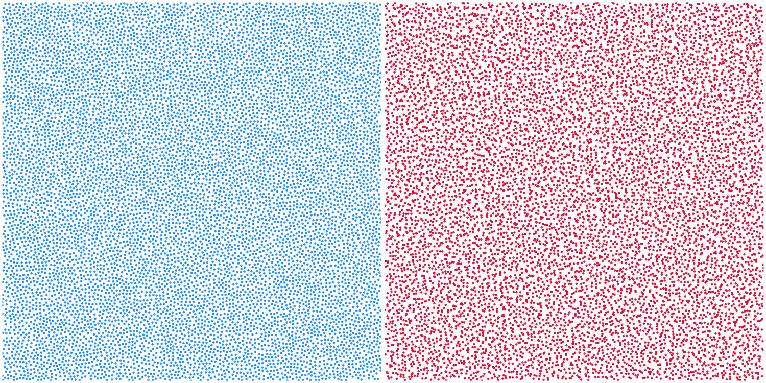
Figure 1: Realizations of a non-hyperuniform (left) and a hyperuniform (right) point process, both with about 10000 points.

To highlight how difficult it can be to distinguish a hyperuniform point pattern from a non-hyperuniform one by eye, Figure 1 is illustrative. The left hand figure shows a realization of a (non-hyperuniform) Matérn III process close to saturation [10]. While this process exhibits a high degree of local order, it possesses Poisson-like long-range density fluctuations that are incompatible with hyperuniformity. In juxtaposition, the right hand figure illustrates a hyperuniform process. To construct this sample, we first simulated a stealthy hyperuniform point pattern [39] and then perturbed each point — independently of each other — according to a Gaussian distribution. Both processes have been simulated on the flat torus. The subtle difference in the long-range order of the two samples is clearly detected by the novel test statistic. This statistic takes a value larger than 300 for the non-hyperuniform sample, i.e., it strongly exceeds the critical value of 2.39, which corresponds to a nominal significance level of 5%. In contrast, the test statistic attains the value 0.04 for the hyperuniform sample. This fact clearly demonstrates a striking sensitivity of our test for hyperuniformity.

In the following, we summarize our results and relate them to the relevant literature. In Section 2, we introduce a few key concepts from the theory of stationary point processes, and we define hyperuniformity. Following the classical reference [6] (see also the recent survey [23]), Section 3 introduces the empirical Fourier transform of a point process, defined in terms of a rather general taper function. Proposition 3.3 provides the asymptotic covariance structure of this transform. At least implicitly, the special case $d=1$ has been dealt with in [6]. Even though this structure might be considered part of the folklore in spatial statistics, we are not aware of a rigorously proved result for a general dimension. A related paper is [19], where the authors study bias and variance of kernel estimators of the asymptotic variance. In Section 4, we establish a multivariate central limit theorem (CLT) for the empirical Fourier transform (see Theorem 4.1), thus extending a result of [6] to general dimensions. And as in [6] we do so under an assumption on the reduced factorial cumulant measures. Our proof does also benefit from the classical source [22], where the authors adopt a similar hypothesis to establish a related CLT; see also [21] for a more recent contribution to the asymptotic normality of kernel estimators of correlation functions. We illustrate our result with Poisson cluster and $\alpha$-determinantal processes.

In what follows, we use the empirical scattering intensity (2.13) as a well-established estimator of the structure factor; see [39]. Section 5 discusses its multivariate asymptotic behavior for different wave vectors and for large system sizes. It will be seen that the resulting limit distribution is made up of exponential random variables which are independent for different wave vectors (Proposition 5.4). This crucial result requires the underlying point process to satisfy the multivariate central limit theorem (5.2). On the theoretical side, this assumption is supported by our Theorem 4.1 and by [4, Theorem 1]; see Remark 5.3. Moreover, we have simulated six models (two of which are hyperuniform) across the first three dimensions. In each of these cases we observed the theoretically predicted behavior over up to six orders of magnitude already for small system sizes of about 1000 points. Hence, our simulations indicate a fast speed of convergence, so that the asymptotic distribution is attained with high accuracy at practically relevant system sizes.

In Section 6, we abandon the background of point processes and adopt the asymptotic setting of Proposition 5.4. By taking a quadratic parametrization (2.9) of the structure factor, we obtain a statistical model with only two parameters $s$ and $t$ (say). This additional approximation and simplification can be justified by taking sufficiently large system sizes. Hyperuniformity is then characterized by the equation $s=0$, which defines our null hypothesis $H_{0}$. Next we introduce maximum likelihood estimators (MLEs) $\widehat{t}_{0}$ of $t$ under the null hypothesis and $(\widehat{s},\widehat{t}_{1})$ of $(s,t)$ for the full model, respectively. Under $H_{0}$, the estimator $\widehat{t}_{0}$ of $t$, when applied to random data, is unbiased and consistent. For finite system sizes, it follows an exact gamma distribution. Under the full model we observe that, asymptotically, the distribution of $\widehat{s}$ equals a mixture of the Dirac distribution in $0$ and a gamma distribution, while $\widehat{t}_{1}$ follows a gamma distribution. In particular the distribution of $\widehat{s}$ has an atom in $0$. These findings are based on numerical solutions for the likelihood equations and on extensive simulations.

In Section 7, we introduce our likelihood ratio test. Working in the asymptotic and parametric setting of Section 6, we consider the ratio of the maximum likelihood of the data under the hypothesis and the corresponding maximum likelihood over the full parameter space. The resulting test statistic is twice the negative logarithm of this ratio. Analytically, the asymptotic distribution of this test statistic seems to be out of reach. Again we have run extensive simulations to obtain this distribution with high accuracy. Under the hypothesis, this limit distribution is a mixture of an atom at $0$ (inherited from the atom of $\widehat{s}$) and a gamma distribution, and it turns out that it does already apply for rather moderate system sizes. Moreover, we show rigorously that this limit distribution does not depend on the actual value of the parameter $t$. Therefore we obtain a significance test for hyperuniformity which can conveniently be used to spatial point patterns occurring in applications.

In Section 8 we apply our test to independent thinnings of the matching process from [32]; see also Example (v) in Section 5. The introduction of a thinning parameter is a convenient way of tuning the parameter $s$. The hyperuniform case $s=0$ arises in the limit case of no thinning. It turns out that the asymptotic distribution of the test statistic applies extremely well to this point process. Remarkably, it does so for only one sample with moderately large system size. We apply our test with a nominal significance level of 0.05 for different values of the parameter $s$. If $s=0$ the test keeps this nominal level very well. Already for $s=10^{-3}$ and a system size of $L=150$ the test rejects hyperuniformity in almost all cases. Even for $s=10^{-4}$, which is an order of magnitude smaller than typical non-hyperuniform models (see [39, 31]), the rejection rate increases dramatically with growing systems size; see Table 1 for more details.

We finish the paper with some remarks on the principles underlying our test, and we also formulate some interesting further problems and tasks.

2 Preliminaries

We first introduce some point process terminology, most of which can be found in Chapters 8 and 9 from [34]. We work on ${\mathbb{R}}^{d}$, $d\geq 1$, equipped with the Borel $\sigma$-field ${\mathcal{B}}^{d}$ and Lebesgue measure $\lambda_{d}$. Let ${\mathcal{B}}^{d}_{b}$ be the bounded elements of ${\mathcal{B}}^{d}$, and write ${\mathbf{N}}$ for the system of locally finite subsets of ${\mathbb{R}}^{d}$. For $\mu\in{\mathbf{N}}$ and $B\subset{\mathbb{R}}^{d}$ we denote by $\mu(B)$ the cardinality of $\mu\cap B$. By definition, we have $\mu(B)\in{\mathbb{N}}_{0}$ for each $B\in{\mathcal{B}}^{d}_{b}$. Let $\mathcal{N}$ be the smallest $\sigma$-field on ${\mathbf{N}}$ that renders the mappings $\mu\mapsto\mu(B)$ measurable for each $B\in{\mathcal{B}}^{d}$.

A (simple) point process is a random element $\eta$ of $({\mathbf{N}},\mathcal{N})$, defined on some fixed probability space $(\Omega,\mathcal{F},\mathbb{P})$ with associated expectation operator $\mathbb{E}$. The process is called stationary if the distribution of $\eta+x:=\{y+x:y\in\eta\}$ does not depend on $x\in{\mathbb{R}}^{d}$. In this case $\gamma:=\mathbb{E}\eta([0,1]^{d})$ is called the intensity or – in the terminology of physics – the number density of $\eta$. By Campbell’s formula,

$$\mathbb{E}\sum_{x\in\eta}f(x)=\gamma\int f(x)\,{\text{d}}x$$ (2.1)

for each measurable function $f\colon{\mathbb{R}}^{d}\to[0,\infty)$. Here and in what follows, each unspecified integral is over the full domain.

We consider a stationary point process $\eta$ with positive and finite intensity $\gamma$. We assume that $\eta$ is locally square integrable, i.e., $\mathbb{E}\eta(B)^{2}<\infty$ for each $B\in{\mathcal{B}}^{d}_{b}$. The reduced second factorial moment measure $\alpha^{!}_{2}$ of $\eta$ is defined by the formula

$$\alpha^{!}_{2}(\cdot):=\mathbb{E}\sideset{}{{}^{\neq}}{\sum}_{x,y\in\eta}{\mathbf{1}}\big{\{}x\in[0,1]^{d},y-x\in\cdot\big{\}}.$$

Here, the superscript $\neq$ indicates summation over pairs with different components, and ${\mathbf{1}}\{\cdot\}$ stands for the indicator function. Notice that $\alpha^{!}_{2}$ is a locally finite measure on ${\mathbb{R}}^{d}$, which is invariant under reflections at the origin and satisfies the equation

$$\mathbb{E}\sideset{}{{}^{\neq}}{\sum}_{x,y\in\eta}{\mathbf{1}}\{(x,y)\in\cdot\}=\iint{\mathbf{1}}\{(x,x+y)\in\cdot\}\,\alpha^{!}_{2}({\text{d}}y)\,{\text{d}}x.$$ (2.2)

Quite often the measure $\alpha^{!}_{2}$ has a density (w.r.t. Lebesgue measure), which gives

$$\alpha^{!}_{2}({\text{d}}y)=\gamma^{2}g_{2}(y)\,{\text{d}}y,$$

where $g_{2}\colon{\mathbb{R}}^{d}\to[0,\infty)$ is the so-called pair correlation function of $\eta$. This function is measurable and locally integrable, and it can be assumed to satisfy $g_{2}(x)=g_{2}(-x)$ for each $x\in{\mathbb{R}}^{d}$. Given $B\in{\mathcal{B}}^{d}$, it follows from (2.2) that

$$\mathbb{E}\eta(B)^{2}=\gamma\lambda_{d}(B)+\iint{\mathbf{1}}\{x\in B,x+y\in B\}\,{\text{d}}x\,\alpha^{!}_{2}({\text{d}}y);$$

see [34, (4.25) and (8.8)]. If $B$ is bounded, then the variance of $\eta(B)$ is

$$\operatorname{{\mathbb{V}ar}}\eta(B)=\gamma\lambda_{d}(B)+\int\lambda_{d}(B\cap(B+y))\,\alpha^{!}_{2}({\text{d}}y)-\gamma^{2}\lambda_{d}(B)^{2}.$$

Since $\int\lambda_{d}(B\cap(B+y))\,{\text{d}}y=\lambda_{d}(B)^{2}$, an alternative representation is

$$\operatorname{{\mathbb{V}ar}}\eta(B)=\gamma\lambda_{d}(B)+\int\lambda_{d}(B\cap(B+y))\,\beta^{!}_{2}({\text{d}}y),$$ (2.3)

where the signed measure $\beta^{!}_{2}$ is given by

$$\beta^{!}_{2}:=\alpha^{!}_{2}-\gamma^{2}\lambda_{d}.$$ (2.4)

In accordance with [5, Chapter 9], we call $\beta^{!}_{2}$ the covariance measure of $\eta$. In fact, the measure $\beta^{!}_{2}$ is the second reduced factorial cumulant measure of $\eta$, which is a special case of a locally finite measure $\beta^{!}_{m}$ defined in (4.6) for each integer $m\geq 2$. The covariance measure is only defined on the system of bounded Borel sets of ${\mathbb{R}}^{d}$. The restriction $\beta^{!}_{2}(B\cap\cdot)$ of $\beta^{!}_{2}$ onto a bounded Borel subset $B$ of ${\mathbb{R}}^{d}$ is a finite signed measure and hence can be written as the difference of two orthogonal finite measures. In this way, we can define the total variation measure $|\beta^{!}_{2}|$, first on $B$, and then by consistency on each Borel set. The result is a locally finite measure on ${\mathbb{R}}^{d}$. If $\eta$ has a pair correlation function $g_{2}$, then

$$\beta^{!}_{2}({\text{d}}x)=\gamma^{2}(g_{2}(x)-1)\,{\text{d}}x$$

and

$$|\beta^{!}_{2}|({\text{d}}x)=\gamma^{2}|g_{2}(x)-1|\,{\text{d}}x.$$

In Sections 3 and 4 we shall assume that

$$|\beta^{!}_{2}|({\mathbb{R}}^{d})<\infty.$$ (2.5)

Let $W\subset{\mathbb{R}}^{d}$ be a convex compact set with non-empty interior. For each $y\in{\mathbb{R}}^{d}$ we have $\lim_{r\to\infty}\lambda_{d}(rW)^{-1}\lambda_{d}(rW\cap(rW+y))=1$. If (2.5) holds, we therefore obtain from (2.3) and dominated convergence that

$$\lim_{r\to\infty}\frac{\operatorname{{\mathbb{V}ar}}\eta(rW)}{\lambda_{d}(rW)}=\gamma+\gamma^{2}\beta^{!}_{2}({\mathbb{R}}^{d}).$$ (2.6)

The point process $\eta$ is said to be hyperuniform w.r.t. $W$ if

$$\lim_{r\to\infty}\frac{\operatorname{{\mathbb{V}ar}}\eta(rW)}{\lambda_{d}(rW)}=0.$$

If this convergence holds with $W$ given by the unit ball $B_{1}:=\{x\in{\mathbb{R}}^{d}:\|x\|\leq 1\}$, where $\|\cdot\|$ denotes the Euclidean norm, then we just say that $\eta$ is hyperuniform [41, 39]. If (2.5) holds, then (2.6) shows that hyperuniformity is equivalent to

$$\gamma\beta^{!}_{2}({\mathbb{R}}^{d})=-1.$$ (2.7)

In this paragraph we assume that (2.5) holds. Writing ${\mathrm{i}}$ for the imaginary unit and $\langle\cdot,\cdot\rangle$ for the inner product on ${\mathbb{R}}^{d}\times{\mathbb{R}}^{d}$, the structure factor $S$ of $\eta$ is the function on ${\mathbb{R}}^{d}$ defined by

$$S(k):=1+\frac{1}{\gamma}\int{\mathrm{e}}^{-{\mathrm{i}}\langle k,x\rangle}\,\beta_{2}^{!}({\text{d}}x),\quad k\in{\mathbb{R}}^{d}.$$ (2.8)

This definition is justified by assumption (2.5). If $\eta$ has a pair correlation function, then the structure factor is given by

$$S(k)=1+\gamma\int{\mathrm{e}}^{-{\mathrm{i}}\langle k,x\rangle}(g_{2}(x)-1)\,{\text{d}}x,\quad k\in{\mathbb{R}}^{d},$$

which means that $\gamma^{-1}(S-1)$ is the Fourier transform of $g_{2}-1$. In the general case, $\gamma^{-1}(S-1)$ is the Fourier transform of the covariance measure. Since $\beta_{2}^{!}$ is invariant with respect to reflections, the function $S$ is real-valued, and we have $S(k)=S(-k)$ for each $k\in{\mathbb{R}}^{d}$. Hyperuniformity is equivalent to

$$S(0)=0.$$

Notice that the symbol $0$ stands for the origin in ${\mathbb{R}}^{d}$ for each $d\geq 1$ and thus in particular for the real number zero. The specific meaning will always be clear from the context. Assuming that there exists an isotropic pair correlation function satisfying

$$\int\|x\|^{2}|g_{2}(x)-1|\,{\text{d}}x<\infty,$$

we can write

$$S(k)=s+t\|k\|^{2}+o(\|k\|^{2}),\quad\text{as $k\to 0$}.$$ (2.9)

In the important special case of a perturbed lattice, assumption (2.5) is not satisfied; see e.g. [30]. In order to define the structure factor also in such cases, we assume that

$$\beta^{!}_{2}=\beta^{c}_{2}+\beta^{d}_{2},$$ (2.10)

where $\beta^{c}_{2}$ and $\beta^{d}_{2}$ are signed measures with the following properties. The measure $\beta^{c}_{2}$ is the difference of two signed positive semidefinite measures (see [2, Section 1.4]) of finite total variation. As for $\beta_{2}^{d}$, we suppose that there exists a lattice $\mathbb{L}\subset{\mathbb{R}}^{d}$ and a probability measure $\mathbb{Q}$ on ${\mathbb{R}}^{d}$ such that

$$\beta^{d}_{2}=\sum_{q\in\mathbb{L}}\iint{\mathbf{1}}\{q+x-y\in\cdot\}\,\mathbb{Q}({\text{d}}x)\,\mathbb{Q}({\text{d}}y)-\lambda_{d}.$$ (2.11)

Under these assumptions, we can define the structure factor by (2.8) with $\beta^{c}_{2}$ instead of $\beta^{!}_{2}$. If (2.9) holds, hyperuniformity is still equivalent to $S(0)=0$. This claim can be proved with the Fourier methods from [2]. For the perturbed lattice, $\mathbb{Q}$ is the distribution of the perturbation, and (2.9) holds provided that $\int\|x\|\,\mathbb{Q}({\text{d}}x)<\infty$. More generally, we can replace (2.11) by

$$\beta^{d}_{2}=\sum_{q\in\mathbb{L}}\iint{\mathbf{1}}\{q+x\in\cdot\}\,\mathbb{Q}^{\prime}({\text{d}}x)-\lambda_{d},$$ (2.12)

where $\mathbb{Q}^{\prime}$ is a positive semidefinite probability measure.

Assuming that (2.9) holds, we will test the hypothesis $S(0)=0$ (i.e., hyperuniformity) using the empirical scattering intensity

$$\mathcal{S}_{r}(k):=\frac{1}{\eta(W_{r})}\bigg{|}\sum_{x\in\eta\cap W_{r}}{\mathrm{e}}^{-{\mathrm{i}}\langle k,x\rangle}-{\mathbf{1}}\{k=0\}\gamma r^{d}\bigg{|}^{2},\quad k\in{\mathbb{R}}^{d},$$ (2.13)

where $0^{-1}:=0$ and $W_{r}$ is a cube centered at $0$ with side length $r>0$.

3 Asymptotic covariance structure

In this section we assume that

$$\int(1+\|x\|)\,|\beta^{!}_{2}|({\text{d}}x)<\infty,$$ (3.1)

which strengthens (2.5).

We fix a bounded and measurable function $h\colon{\mathbb{R}}^{d}\to[0,\infty)$ satisfying

$$M_{1}(h)<\infty,$$ (3.2)

where

$$M_{j}(h):=\int h(x)^{j}\,{\text{d}}x,\quad j=1,2.$$

Since $h$ is bounded, we also have $M_{2}(h)<\infty$. For $r>0$ set $h_{r}(x):=h(x/r)$ and note that $\int h_{r}(x)^{j}\,{\text{d}}x=M_{j}(h)r^{d}$ for $j\in\{1,2\}$. We assume that

$$\lim_{r\to\infty}\frac{1}{r^{d}}\int h_{r}(x)^{2}{\mathrm{e}}^{{\mathrm{i}}\langle k,x\rangle}\,{\text{d}}x=0,\quad k\in{\mathbb{R}}^{d}\setminus\{0\}.$$ (3.3)

We further suppose that there is a set $A_{h}\subset{\mathbb{R}}^{d}\setminus\{0\}$ such that $A_{h}=-A_{h}$ and

$$\lim_{r\to\infty}\frac{1}{r^{d/2}}\int h_{r}(x){\mathrm{e}}^{{\mathrm{i}}\langle k,x\rangle}\,{\text{d}}x=0,\quad k\in A_{h}.$$ (3.4)

Finally, we assume that there exist $a,b>0$ such that

$$\int|h(x+y)-h(x)|\,{\text{d}}x\leq a{\mathbf{1}}\{\|y\|\leq b\}\|y\|+a{\mathbf{1}}\{\|y\|>b\},\quad y\in{\mathbb{R}}^{d}.$$ (3.5)

Example 3.1.

Let $B_{r}\subset{\mathbb{R}}^{d}$ denote the closed ball with radius $r$, centered at the origin, and let $r_{d}>0$ be such that $\kappa_{d}r_{d}^{d}=1$, where $\kappa_{d}\,(=\pi^{d/2}/\Gamma(1+d/2))$ is the volume of a ball with radius $1$ and $\Gamma(\cdot)$ denotes the Gamma function. Let $h$ be the indicator function of $B_{r_{d}}$. Then $M_{1}(h)=M_{2}(h)=1$, and $h_{r}$ is the indicator function of a ball with radius $rr_{d}$. As for (3.4), we need a classical fact regarding the Fourier transform of the indicator function of a ball; see e.g. [17, Section B.5]. For each $r>0$ we have

$$\int_{B_{r}}{\mathrm{e}}^{{\mathrm{i}}\langle k,x\rangle}\,{\text{d}}x=\Big{(}\frac{2\pi r}{\|k\|}\Big{)}^{d/2}J_{d/2}(\|k\|r),\quad k\in{\mathbb{R}}^{d}\setminus\{0\},$$

where, for $a>-1/2$, the Bessel function of the first kind $J_{a}\colon[0,\infty)\to{\mathbb{R}}$ is given by

$$J_{a}(t):=\sum^{\infty}_{m=0}\frac{(-1)^{m}}{m!\Gamma(m+a+1)}\Big{(}\frac{t}{2}\Big{)}^{2m+a},\quad t\geq 0.$$

Since $\lim_{t\to\infty}J_{a}(t)=0$ (see  [17, Section B.8]), we obtain (3.3) and (3.4) for $A_{h}:={\mathbb{R}}^{d}\setminus\{0\}$.

To check (3.5), put $a_{+}:=\max(0,a)$ for $a\in{\mathbb{R}}$ and note that for each $y\in{\mathbb{R}}^{d}$

$$\int {\mathbf{1}}\{x\in B_{r_{d}},x+y\notin B_{r_{d}}\}\,{\text{d}}x$$

$$\leq{\mathbf{1}}\{\|y\|\leq r_{d}\}\int{\mathbf{1}}\{x\in B_{r_{d}}\setminus B_{(r_{d}-\|y\|)_{+}}\}\,{\text{d}}x+{\mathbf{1}}\{\|y\|>r_{d}\}.$$

The first term can be bounded by

$${\mathbf{1}}\{\|y\|\leq r_{d}\}\big{(}\kappa_{d}r_{d}^{d}-\kappa_{d}(r_{d}-\|y\|)^{d}\big{)} \leq{\mathbf{1}}\{\|y\|\leq r_{d}\}\sum_{j=0}^{d-1}c_{j}r_{d}^{j}\|y\|^{d-j}$$

$$\leq{\mathbf{1}}\{\|y\|\leq r_{d}\}\|y\|\sum_{j=0}^{d-1}c_{j}r_{d}^{d-j-1}$$

for some positive constants $c_{0},\ldots,c_{d-1}$. Since the same bound applies to

$$\int{\mathbf{1}}\{x\notin B_{r_{d}},x+y\in B_{r_{d}}\}\,{\text{d}}x=\int{\mathbf{1}}\{x-y\notin B_{r_{d}},x\in B_{r_{d}}\}\,{\text{d}}x,$$

(3.5) follows.

Example 3.2.

Assume that $h$ is the indicator function of the unit cube $W_{1}:=[-1/2,1/2]^{d}$, centered at the origin. Then $M_{1}(h)=M_{2}(h)=1$, and $h_{r}$ is the indicator function of the cube $W_{r}:=[-r/2,r/2]^{d}$. An easy calculation gives

$$\int_{W_{r}}{\mathrm{e}}^{{\mathrm{i}}kx}\,{\text{d}}x=\prod^{d}_{j=1}\frac{2}{k_{j}}\sin\frac{k_{j}r}{2},\quad k=(k_{1},\ldots,k_{d})\in{\mathbb{R}}^{d},$$

where we set $\sin st/s:=t$ for $s=0$. Hence (3.3) holds, while (3.4) is valid with $A_{h}$ given by

$$A_{\Box}:=\bigg{\{}x\in{\mathbb{R}}^{d}:\sum^{d}_{i=1}{\mathbf{1}}\{|x_{i}|>0\}\geq\frac{d}{2}\bigg{\}}.$$ (3.6)

If $d=2$, then $A_{\Box}={\mathbb{R}}^{2}\setminus\{0\}$. Relation (3.5) can be checked as in Example 3.1. We leave this check to the reader.

Similarly as in [6] we define for each $r>0$ a random function $T_{r}$ on ${\mathbb{R}}^{d}$ by

$$T_{r}(k):=\frac{1}{r^{d/2}}\sum_{x\in\eta}h_{r}(x){\mathrm{e}}^{-{\mathrm{i}}\langle k,x\rangle}-{\mathbf{1}}\{k=0\}M_{1}(h)\gamma r^{d/2},\quad k\in{\mathbb{R}}^{d}.$$ (3.7)

In the language of point process theory, $T_{r}(k)$ is a linear function of $\eta$. Note that $T_{r}(-k)$ equals the conjugate $\overline{T_{r}(k)}$ of $T_{r}(k)$. In the case of Example 3.2, $T_{r}$ is closely related to the scattering intensity (2.13). In this connection, the function $h$ figuring in (3.2) is called a taper function; see [6]. In physics, the variables (3.7) are known as collective coordinates; see [42]. From Campbell’s formula (2.1) and (3.4) we obtain

$$\lim_{r\to\infty}\mathbb{E}T_{r}(k)=0,\quad k\in{\mathbb{R}}^{d}.$$ (3.8)

In fact, if $k=0$ then $\mathbb{E}T_{r}(k)=0$ for each $r>0$. The following result provides the asymptotic behavior of the covariances of the functionals $T_{r}$.

Proposition 3.3.

Let $k,\ell\in A_{h}\cup\{0\}$. Then

$$\lim_{r\to\infty}\mathbb{E}T_{r}(k)\overline{T_{r}(\ell)}={\mathbf{1}}\{k=\ell\}\gamma M_{2}(h)S(k).$$ (3.9)

Proof.

Let $k,\ell\in A_{h}\cup\{0\}$. We first assume that $k\neq 0$ and $\ell\neq 0$. Then

$$\mathbb{E}T_{r}(k)\overline{T_{r}(\ell)} =\frac{1}{r^{d}}\mathbb{E}\bigg{[}\sum_{x,y\in\eta}h_{r}(x)h_{r}(y){\mathrm{e}}^{-{\mathrm{i}}\langle k,x\rangle}{\mathrm{e}}^{{\mathrm{i}}\langle\ell,y\rangle}\bigg{]}$$

$$=\frac{1}{r^{d}}\mathbb{E}\bigg{[}\sum_{x\in\eta}h_{r}(x)^{2}{\mathrm{e}}^{-{\mathrm{i}}\langle k,x\rangle}{\mathrm{e}}^{{\mathrm{i}}\langle\ell,x\rangle}\bigg{]}+\frac{1}{r^{d}}\mathbb{E}\bigg{[}\sideset{}{{}^{\neq}}{\sum}_{x,y\in\eta}h_{r}(x)h_{r}(y){\mathrm{e}}^{-{\mathrm{i}}\langle k,x\rangle}{\mathrm{e}}^{{\mathrm{i}}\langle\ell,y\rangle}\bigg{]}.$$

By Campbell’s formula (2.1) and (2.2) this means that

$$\mathbb{E}T_{r}(k)\overline{T_{r}(\ell)} =\frac{\gamma}{r^{d}}\int h_{r}(x)^{2}{\mathrm{e}}^{{\mathrm{i}}\langle\ell-k,x\rangle}\,{\text{d}}x$$

$$\quad+\frac{1}{r^{d}}\iint h_{r}(x)h_{r}(x+y){\mathrm{e}}^{-{\mathrm{i}}\langle k,x\rangle}{\mathrm{e}}^{{\mathrm{i}}\langle\ell,x+y\rangle}\,{\text{d}}x\,\alpha^{!}_{2}({\text{d}}y)$$ (3.10)

$$=:C_{1}(r)+C_{2}(r),$$

say. By (3.3) we have

$$\lim_{r\to\infty}C_{1}(r)=\gamma M_{2}(h){\mathbf{1}}\{k=\ell\}.$$

Assumption (3.4) shows that

$$\lim_{r\to\infty}C_{2}(r)=\lim_{r\to\infty}C^{\prime}_{2}(r),$$

where

$$C^{\prime}_{2}(r):=\frac{1}{r^{d}}\iint h_{r}(x)h_{r}(x+y){\mathrm{e}}^{-{\mathrm{i}}\langle k,x\rangle}{\mathrm{e}}^{{\mathrm{i}}\langle\ell,x+y\rangle}\,{\text{d}}x\,\beta^{!}_{2}({\text{d}}y).$$

We have

$$C^{\prime}_{2}(r) =\frac{1}{r^{d}}\iint h_{r}(x)h_{r}(x+y){\mathrm{e}}^{{\mathrm{i}}\langle\ell-k,x\rangle}{\mathrm{e}}^{{\mathrm{i}}\langle\ell,y\rangle}\,{\text{d}}x\,\beta^{!}_{2}({\text{d}}y)$$

$$=\frac{1}{r^{d}}\iint h_{r}(x)^{2}{\mathrm{e}}^{{\mathrm{i}}\langle\ell-k,x\rangle}{\mathrm{e}}^{{\mathrm{i}}\langle\ell,y\rangle}\,{\text{d}}x\,\beta^{!}_{2}({\text{d}}y)$$

$$\qquad+\frac{1}{r^{d}}\iint h_{r}(x)(h_{r}(x+y)-h_{r}(x)){\mathrm{e}}^{{\mathrm{i}}\langle\ell-k,x\rangle}{\mathrm{e}}^{{\mathrm{i}}\langle\ell,y\rangle}\,{\text{d}}x\,\beta^{!}_{2}({\text{d}}y)$$

$$=:D_{1}(r)+D_{2}(r),$$

say. Furthermore,

$$D_{1}(r)=\frac{1}{r^{d}}\int h_{r}(x)^{2}{\mathrm{e}}^{{\mathrm{i}}\langle\ell-k,x\rangle}\,{\text{d}}x\int{\mathrm{e}}^{i\langle\ell,y\rangle}\,\beta^{!}_{2}({\text{d}}y).$$

If $k=\ell$ then this expression equals

$$M_{2}(h)\int{\mathrm{e}}^{{\mathrm{i}}\langle k,y\rangle}\,\beta^{!}_{2}({\text{d}}y)=M_{2}(h)\gamma^{-1}(S(k)-1).$$

From (3.3), we otherwise obtain $D_{1}(r)\to 0$ as $r\to\infty$.

We now show that $D_{2}(r)\to 0$ as $r\to\infty$. Let $c>0$ be an upper bound of $|h|$. Then, using (3.5), we have

$$|D_{2}(r)|\leq\frac{c}{r^{d}} \iint|h_{r}(x+y)-h_{r}(x)|\,{\text{d}}x\,|\beta^{!}_{2}|({\text{d}}y)$$

$$=c\iint|h(x+r^{-1}y)-h_{r}(x)|\,{\text{d}}x\,|\beta^{!}_{2}|({\text{d}}y)$$

$$\leq ca\int r^{-1}\|y\|\,|\beta^{!}_{2}|({\text{d}}y)+\gamma^{2}a\int{\mathbf{1}}\{\|y\|>rb\}\,|\beta^{!}_{2}|({\text{d}}y).$$

By (3.1) and (2.5) this upper bound tends to zero as $r\to\infty$.

It remains to deal with the case $k=0$. If $k=0$ then

$$\mathbb{E}T_{r}(0)T_{r}(\ell) =\frac{1}{r^{d}}\mathbb{E}\bigg{[}\sum_{y\in\eta}h_{r}(y)\sum_{x\in\eta}h_{r}(x){\mathrm{e}}^{-{\mathrm{i}}\langle\ell,x\rangle}\bigg{]}-M_{1}(h)\gamma\mathbb{E}\bigg{[}\sum_{x\in\eta}h_{r}(x){\mathrm{e}}^{-{\mathrm{i}}\langle\ell,x\rangle}\bigg{]}$$

$$=\frac{\gamma}{r^{d}}\int h_{r}(x)^{2}{\mathrm{e}}^{-{\mathrm{i}}\langle\ell,x\rangle}\,{\text{d}}x+\frac{1}{r^{d}}\iint{\mathrm{e}}^{-{\mathrm{i}}\langle\ell,x\rangle}h_{r}(x)h_{r}(x+y)\,{\text{d}}x\,\alpha^{!}_{2}({\text{d}}y)$$

$$\quad-M_{1}(h)\gamma^{2}\int h_{r}(x){\mathrm{e}}^{-{\mathrm{i}}\langle\ell,x\rangle}\,{\text{d}}x.$$

Since $\int h_{r}(x+y)\,{\text{d}}y=M_{1}(h)r^{d}$, $x\in{\mathbb{R}}^{d}$, we obtain

$$\mathbb{E}T_{r}(0)T_{r}(\ell)=\frac{\gamma}{r^{d}}\int h_{r}(x)^{2}{\mathrm{e}}^{-{\mathrm{i}}\langle\ell,x\rangle}\,{\text{d}}x+\frac{1}{r^{d}}\iint{\mathrm{e}}^{-{\mathrm{i}}\langle\ell,x\rangle}h_{r}(x)h_{r}(x+y)\,{\text{d}}x\,\beta^{!}_{2}({\text{d}}y).$$

If $\ell=0$, the first term equals $\gamma M_{2}(h)$. Otherwise, it tends to zero by (3.3). Similarly as before we write the second term as

$$\frac{1}{r^{d}}\beta^{!}_{2}({\mathbb{R}}^{d})\int{\mathrm{e}}^{-{\mathrm{i}}\langle\ell,x\rangle}h_{r}(x)^{2}\,{\text{d}}x+\frac{1}{r^{d}}\iint{\mathrm{e}}^{-{\mathrm{i}}\langle\ell,x\rangle}h_{r}(x)(h_{r}(x+y)-h_{r}(x))\,{\text{d}}x\,\beta^{!}_{2}({\text{d}}y).$$

Here, the second term tends to $0$ as $r\to\infty$, and so does the first if $\ell\neq 0$. If $\ell=0$ the first term equals $M_{2}(h)\beta^{!}_{2}({\mathbb{R}}^{d})=M_{2}(h)\gamma^{-1}(S(0)-1)$. ∎

Later we shall use the following non-asymptotic result.

Corollary 3.4.

Let $r>0$ and $k\in{\mathbb{R}}^{d}\setminus\{0\}$. Then

$$\mathbb{E}|T_{r}(k)|^{2} =\gamma M_{2}(h)S(k)+\frac{1}{r^{d}}\iint h_{r}(x)(h_{r}(x+y)-h_{r}(x)){\mathrm{e}}^{{\mathrm{i}}\langle k,y\rangle}\,{\rm d}x\,\beta^{!}_{2}(\text{{\rm d}}y)$$

$$\quad+\frac{\gamma^{2}}{r^{d}}\bigg{|}\int h_{r}(x){\mathrm{e}}^{-{\mathrm{i}}\langle k,x\rangle}\,\text{{\rm d}}x\bigg{|}^{2}.$$ (3.11)

Proof.

By (3),

$$\mathbb{E}|T_{r}(k)|^{2}=\gamma M_{2}(h)+\frac{1}{r^{d}}\iint h_{r}(x)h_{r}(x+y){\mathrm{e}}^{{\mathrm{i}}\langle k,y\rangle}\,{\text{d}}x\,\alpha^{!}_{2}({\text{d}}y),$$

which in view of (2.4) can be written as

$$\mathbb{E}|T_{r}(k)|^{2}=\gamma M_{2}(h)+A_{r}+B_{r},$$

where

$$A_{r} :=\frac{1}{r^{d}}\iint h_{r}(x)h_{r}(x+y){\mathrm{e}}^{{\mathrm{i}}\langle k,y\rangle}\,{\text{d}}x\,\beta^{!}_{2}({\text{d}}y),$$

$$B_{r} :=\frac{\gamma^{2}}{r^{d}}\iint h_{r}(x)h_{r}(x+y)e^{-{\mathrm{i}}\langle k,y\rangle}\,{\text{d}}x\,{\text{d}}y.$$

Since ${\mathrm{e}}^{{\mathrm{i}}\langle k,y\rangle}={\mathrm{e}}^{{\mathrm{i}}\langle k,x\rangle}{\mathrm{e}}^{-{\mathrm{i}}\langle k,x+y\rangle}$, $B_{r}$ equals the third term on the right-hand side of (3.4). Moreover, we have

$$A_{r}=M_{2}(h)\int{\mathrm{e}}^{{\mathrm{i}}\langle k,y\rangle}\,\beta^{!}_{2}({\text{d}}y)+\frac{1}{r^{d}}\iint h_{r}(x)(h_{r}(x+y)-h_{r}(x)){\mathrm{e}}^{{\mathrm{i}}\langle k,y\rangle}\,{\text{d}}x\,\beta^{!}_{2}({\text{d}}y),$$

which concludes the proof. ∎

For $k\in{\mathbb{R}}^{d}$ and $r>0$ we denote by $T_{r,1}(k)$ the real part and by $T_{r,2}(k)$ the imaginary part of $T_{r}(k)$ and define

$$\sigma_{m,n}(k,\ell):=\lim_{r\to\infty}\mathbb{E}T_{r,m}(k)T_{r,n}(\ell),\quad m,n\in\{1,2\},\,k,\ell\in{\mathbb{R}}^{d}.$$

Let ${\mathbb{R}}^{[d]}\subset{\mathbb{R}}^{d}$ satisfy $|{\mathbb{R}}^{[d]}\cap\{k,-k\}|=1$ for each $k\in{\mathbb{R}}^{d}$, where $|A|$ stands for the cardinality of a set $A$.

Corollary 3.5.

Let $k,\ell\in(A_{h}\cup\{0\})\cap{\mathbb{R}}^{[d]}$. We then have

$$\sigma_{m,n}(k,\ell)={\mathbf{1}}\{m=n,k=\ell\}\frac{\gamma M_{2}(h)S(k)}{2},\quad m,n\in\{1,2\},\,k,\ell\in{\mathbb{R}}^{[d]}.$$ (3.12)

Proof.

By (3.9),

$$\sigma_{1,1}(k,k)+\sigma_{2,2}(k,k)=\gamma M_{2}(h)S(k).$$

If we apply (3.9) with $\ell=-k$ and use $T_{r}(-k)=\overline{T_{r}(k)}$, it follows that

$$\sigma_{1,1}(k,k)-\sigma_{2,2}(k,k)=\sigma_{1,2}(k,k)+\sigma_{2,1}(k,k)=0.$$

Hence, (3.12) is proved for $k=\ell$. Assume now that $k,\ell\in{\mathbb{R}}^{[d]}$ with $k\neq\ell$. Then we can apply (3.9) with $\ell$ and $-\ell$ to obtain $\sigma_{m,n}(k,\ell)=0$ for all $m,n\in\{1,2\}$. ∎

4 A central limit theorem

In this section, let $\eta$ be a stationary point process $\eta$ with intensity $\gamma$ satisfying

$$\mathbb{E}\eta(B)^{m}<\infty$$ (4.1)

for each bounded Borel set $B\subset{\mathbb{R}}^{d}$ and each $m\in{\mathbb{N}}$. We let $h$ and $A_{h}$ be as in the previous section. Let $Z_{k}$, $k\in{\mathbb{R}}^{[d]}$, be independent centered ${\mathbb{C}}$-valued normally distributed random variables. The components of $Z_{k}$ are assumed to be independent and to have variance $\gamma M_{2}(h)S(k)/2$. Here and in the sequel, a normally distributed random variable with variance $0$ is almost surely constant. Putting ${\mathbb{R}}^{\{d\}}:=(A_{h}\cup\{0\})\cap{\mathbb{R}}^{[d]}$, we are interested in the multivariate central limit theorem

$$(T_{r}(k_{1}),\ldots,T_{r}(k_{n}))\overset{d}{\longrightarrow}(Z_{k_{1}},\ldots,Z_{k_{n}}),\quad\text{as $r\to\infty$},\,k_{1},\ldots,k_{n}\in{\mathbb{R}}^{\{d\}},$$ (4.2)

where $\overset{d}{\longrightarrow}$ denotes convergence in distribution. In the case $d=1$, Brillinger (see  [6, Theorem 4.2]) proved that this convergence holds under a suitable assumption on the so-called (reduced) cumulant measures of $\eta$. We shall extend Theorem 4.2 of [6] to general dimensions.

To state our result, we introduce some concepts from the theory of point processes (see, e.g. [11]). For each integer $m$, the $m$-th factorial moment measure of $\eta$ is the measure on $({\mathbb{R}}^{d})^{m}$, defined by

$$\alpha_{m}(\cdot):=\mathbb{E}\sideset{}{{}^{\neq}}{\sum}_{x_{1},\ldots,x_{m}\in\eta}{\mathbf{1}}\{(x_{1},\dots,x_{m})\in\cdot\}.$$

Here, $\neq$ indicates summation over $m$-tuples with pairwise different entries. By assumption (4.1), $\alpha_{m}(B)<\infty$ for each bounded Borel set $B\subset({\mathbb{R}}^{d})^{m}$. If $\alpha_{m}$ has a density $\rho_{m}$ (w.r.t. Lebesgue measure on $({\mathbb{R}}^{d})^{m}$), then $\rho_{m}$ is said to be the $m$-th correlation function of $\eta$. For $j\in[m]:=\{1,\dots,m\}$ we denote by $\Pi_{m,j}$ the system of all partitions $\pi$ of $[m]$ whose cardinality $|\pi|$ equals $j$. The $m$-th factorial cumulant measure $\beta_{m}$ of $\eta$ is the signed measure on $({\mathbb{R}}^{d})^{m}$, given by

$$\beta_{m}(B_{1}\times\cdots\times B_{m}):=\sum^{m}_{j=1}(-1)^{j-1}(j-1)!\sum_{\pi\in\Pi_{m,j}}\prod_{I\in\pi}\alpha_{|I|}(\times_{i\in I}B_{i})$$ (4.3)

for bounded Borel sets $B_{1},\ldots,B_{m}\subset{\mathbb{R}}^{d}$. Note that $\beta_{m}$ is only defined on bounded Borel sets of $({\mathbb{R}}^{d})^{m}$. An equivalent definition is

$$\beta_{m}(B_{1}\times\cdots\times B_{m})=\frac{\partial^{m}}{\partial u_{1}\cdots\partial u_{m}}\log G\Big{(}1+\sum_{j=1}^{m}u_{j}{\mathbf{1}}_{B_{j}}\Big{)}\Big{|}_{u_{1}=\cdots=u_{m}=0},$$ (4.4)

where each of the partial derivatives is to be taken from the left. Here, the generating functional $G$ of $\eta$ is given by

$$G(f):=\mathbb{E}\prod_{x\in\eta}f(x)$$

for each measurable function $f\colon{\mathbb{R}}^{d}\to[0,\infty)$. For instance, we have $\beta_{1}({\text{d}}x)=\gamma{\text{d}}x$ and

$$\beta_{2}({\text{d}}(x,y))=\alpha_{2}({\text{d}}(x,y))-\gamma^{2}{\text{d}}x{\text{d}}y.$$ (4.5)

A density of $\beta_{m}$ (if existing) is called $m$-th cumulant density or $m$-th truncated correlation function of $\eta$.

Assume that $m\geq 2$. Since $\eta$ is stationary, $\beta_{m}$ is invariant under joint shifts, and there exists a locally finite signed measure $\beta^{!}_{m}$ on $({\mathbb{R}}^{d})^{m-1}$ satisfying

$$\beta_{m}(\cdot)=\iint{\mathbf{1}}\{(x,x_{1}+x,\ldots,x_{m-1}+x)\in\cdot\}\,\beta^{!}_{m}({\text{d}}(x_{1},\ldots,x_{m-1}))\,{\text{d}}x.$$ (4.6)

If $m=2$, then (4.5) shows that (4.6) is in accordance with (2.4). By [11, Proposition 12.6.IV], the measure $\beta^{!}_{2}$ is symmetric under reflection at the origin. As in the case $m=2$ we can introduce the total variation measure $|\beta^{!}_{m}|$ of $\beta^{!}_{m}$, which is a locally finite measure on $({\mathbb{R}}^{d})^{m-1}$.

The key assumption in this section is

$$\int(1+\|x_{1}\|)\,|\beta^{!}_{m}|({\text{d}}(x_{1},\ldots,x_{m-1}))<\infty$$ (4.7)

for each $m\geq 2$. This condition is a direct generalization of assumption (2.14) in [6] to general dimensions and stronger than Brillinger mixing. The latter notion requires that $|\beta^{!}_{m}|(({\mathbb{R}}^{d})^{m-1})<\infty$ for each $m\geq 2$; see [22]. If $m=2$ then assumption (4.7) boils down to our previous assumption (3.1).

Theorem 4.1.

Let $\eta$ be a stationary point process satisfying (4.1) and (4.7). Then the multivariate central limit theorem (4.2) holds.

Proof.

We adapt well-known methods to our setting; see e.g. [6, 22] and the references therein. Let $m\in{\mathbb{N}}$, and let $X_{1},\ldots,X_{m}$ be complex-valued random variables such that $\mathbb{E}|X_{j}|^{m}<\infty$ for each $j\in[m]$. Then the (joint) cumulant of these random variables is defined by

$$\operatorname{{\mathbb{C}um}}(X_{1},\ldots,X_{m})=\sum_{\sigma\in\Pi_{m}}(-1)^{|\sigma|-1}(|\sigma|-1)!\prod_{I\in\sigma}\mathbb{E}\prod_{i\in I}X_{i}.$$ (4.8)

For real-valued random variables (4.8) is not the definition but rather a fundamental property; see e.g. [38, Proposition 3.2.1]. As in [6], however, we use (4.8) as a natural multilinear extension of the cumulant to random vectors with complex-valued components. Formula (4.8) can be inverted according to

$$\mathbb{E}X_{1}\cdots X_{m}=\sum_{\sigma\in\Pi_{m}}\prod_{I\in\sigma}\operatorname{{\mathbb{C}um}}\big{(}(X_{j})_{j\in I}\big{)}.$$ (4.9)

For any measurable function $f\colon{\mathbb{R}}^{d}\to{\mathbb{C}}$ we put

$$\eta(f):=\sum_{x\in\eta}f(x).$$

Let $m\in{\mathbb{N}}$ and $f_{1},\ldots,f_{m}\colon{\mathbb{R}}^{d}\to{\mathbb{C}}$ be measurable and bounded functions that vanish outside some bounded set. For $I\subset[m]$ we define $f_{I}\colon{\mathbb{R}}^{d}\to{\mathbb{C}}$ by $f_{I}(x):=\prod_{i\in I}f_{i}(x)$, $x\in{\mathbb{R}}^{d}$. Using (4.8) and arguing as in the proof of [22, Lemma 1], one can show that

$$\operatorname{{\mathbb{C}um}}\big{(}\eta(f_{1}),\ldots,\eta(f_{m})\big{)}=\sum_{n=1}^{m}\sum_{\sigma\in\Pi_{m,n}}\int\prod^{n}_{p=1}f_{I_{p}(\sigma)}(x_{p})\,\beta_{n}({\text{d}}(x_{1},\ldots,x_{n})),$$ (4.10)

where we write $\sigma=\{I_{1}(\sigma),\ldots,I_{n}(\sigma)\}$ for $\sigma\in\Pi_{m,n}$. For the benefit of the reader, and since the argument applies to point processes on a general state space, we give the idea of the proof. Let $I\subset[m]$, and let $\Pi_{I}$ be the set of all partitions of $I$. Then it is not hard to see (see [11, Exercise 5.4.5]) that

$$\mathbb{E}\prod_{i\in I}\eta(f_{i})=\sum_{\pi\in\Pi_{I}}\int\prod_{J\in\pi}f_{J}(x_{J})\,\alpha_{|\pi|}({\text{d}}(x_{J})_{J\in\pi}).$$

Inserting this expression into (4.8) yields

$$\operatorname{{\mathbb{C}um}}\big{(}\eta(f_{1}),\ldots,\eta(f_{m})\big{)}=\sum_{\sigma\in\Pi_{m}}(-1)^{|\sigma|-1}(|\sigma|-1)!\prod_{I\in\sigma}\sum_{\pi\in\Pi_{I}}\int\prod_{J\in\pi}f_{J}(x_{J})\,\alpha_{|\pi|}({\text{d}}(x_{J})_{J\in\pi}).$$

We now write the product over $I\in\sigma$ as a sum over $\pi_{1}\in\Pi_{I_{1}(\sigma)},\ldots,\pi_{|\sigma|}\in\Pi_{I_{|\sigma|}(\sigma)}$ and then swap the summation with that over $\sigma$. This swap results in a sum over $\pi\in\Pi_{m}$, followed by a sum over $\sigma\in\Pi_{\pi}$. Finally, we can use definition (4.3) with $\pi$ instead of $[m]$.

We now take $m\geq 3$ and $k_{1},\ldots,k_{m}\in{\mathbb{R}}^{d}$, and we fix $r>0$. If we apply (4.10) with the functions $f_{j}:=h_{r}{\mathrm{e}}^{-{\mathrm{i}}\langle k_{j},\cdot\rangle}$, $j\in[m]$, the right-hand side of (4.10), say $A(r)$, turns out to be

$$A(r)=\sum_{n=1}^{m}\sum_{\sigma\in\Pi_{m,n}}\int\prod^{n}_{p=1}\prod_{j\in I_{p}(\sigma)}h_{r}(x_{p}){\mathrm{e}}^{-{\mathrm{i}}\langle k_{j},x_{p}\rangle}\,\beta_{n}({\text{d}}(x_{1},\ldots,x_{n})).$$

Putting $k^{\prime}:=k_{1}+\cdots+k_{m}$ and using (4.6), we obtain

$$A(r) =\sum_{n=1}^{m}\sum_{\sigma\in\Pi_{m,n}}\iint\prod_{j\in I_{1}(\sigma)}h_{r}(x){\mathrm{e}}^{-{\mathrm{i}}\langle k_{j},x\rangle}$$

$$\qquad\qquad\times\prod^{n}_{p=2}\prod_{j\in I_{p}(\sigma)}h_{r}(x+x_{p}){\mathrm{e}}^{-{\mathrm{i}}\langle k_{j},x_{p}\rangle}{\mathrm{e}}^{-{\mathrm{i}}\langle k_{j},x\rangle}\,\beta^{!}_{n}({\text{d}}(x_{1},\ldots,x_{n-1}))\,{\text{d}}x$$

$$=\sum_{n=1}^{m}\sum_{\sigma\in\Pi_{m,n}}\iint{\mathrm{e}}^{-{\mathrm{i}}\langle k^{\prime},x\rangle}h_{r}(x)^{|I_{1}(\sigma)|}\prod^{n}_{p=2}\prod_{j\in I_{p}(\sigma)}h_{r}(x+x_{p}){\mathrm{e}}^{-{\mathrm{i}}\langle k_{j},x_{p}\rangle}\,\beta^{!}_{n}({\text{d}}(x_{2},\ldots,x_{n}))\,{\text{d}}x,$$

where the term for $n=1$ has to be interpreted appropriately. If $a_{1},b_{1},\ldots,a_{m},b_{m}\in{\mathbb{R}}$ are bounded in absolute value by $c>1$, then, by the triangle inequality,

$$\Big{|}\prod^{m}_{j=1}a_{j}-\prod^{m}_{j=1}b_{j}\Big{|}\leq\sum^{m}_{j=1}c^{m-j}|a_{j}-b_{j}|\leq mc^{m-1}\sum^{m}_{j=1}|a_{j}-b_{j}|.$$

If $c$ is an upper bound of $|h|$, setting $c^{\prime}:=m^{2}c^{m-1}$ gives

$$\Big{|}h_{r}(x)^{|I_{1}(\sigma)|}\prod^{n}_{p=2}h_{r}(x_{p}+x)^{|I_{p}(\sigma)|}-h_{r}(x)^{m}\Big{|} \leq mc^{m-1}\sum^{n}_{p=2}|I_{p}(\sigma)||h_{r}(x_{p}+x)-h_{r}(x)|$$

$$\leq c^{\prime}\sum^{n}_{p=2}|h_{r}(x_{p}+x)-h_{r}(x)|$$

for each $\sigma\in\Pi_{m,n}$. It follows that $A(r)=A_{1}(r)+A_{2}(r)$, where

$$A_{1}(r):=\sum_{n=1}^{m}\sum_{\sigma\in\Pi_{m,n}}\iint{\mathrm{e}}^{-{\mathrm{i}}\langle k^{\prime},x\rangle}h_{r}(x)^{m}\prod^{n}_{p=2}\prod_{j\in I_{p}(\sigma)}{\mathrm{e}}^{-{\mathrm{i}}\langle k_{j},x_{p}\rangle}\,\beta^{!}_{n}({\text{d}}(x_{2},\ldots,x_{n}))\,{\text{d}}x,$$

and $A_{2}(r)$ satisfies

$$|A_{2}(r)| \leq c^{\prime}\sum^{m}_{n=2}\sum^{n}_{p=2}\iint|h_{r}(x_{p}+x)-h_{r}(x)|\,{\text{d}}x\,|\beta^{!}_{n}|({\text{d}}(x_{2},\ldots,x_{n}))$$

$$=c^{\prime}r^{d}\sum^{m}_{n=2}\sum^{n}_{p=2}\iint|h(r^{-1}x_{p}+x)-h(x)|\,{\text{d}}x\,|\beta^{!}_{n}|({\text{d}}(x_{2},\ldots,x_{n})).$$ (4.11)

By assumption (4.7), and since $\int f(x)^{m}{\text{d}}x<\infty$, we have

$$|A_{1}(r)|\leq c^{\prime\prime}r^{d},\quad r>0,$$ (4.12)

for some $c^{\prime\prime}>0$. Invoking assumption (3.5) we obtain from (4)

$$|A_{2}(r)| \leq ac^{\prime}r^{d-1}\sum^{m}_{n=2}\sum^{n}_{p=2}\int\|x_{p}\|\,|\beta^{!}_{n}|({\text{d}}(x_{2},\ldots,x_{n}))$$

$$\quad+ac^{\prime}r^{d}\sum^{m}_{n=2}\sum^{n}_{p=2}\int{\mathbf{1}}\{\|x_{p}\|>rb\}\,|\beta^{!}_{n}|({\text{d}}(x_{2},\ldots,x_{n}))$$

$$=ac^{\prime}r^{d-1}\sum^{m}_{n=2}(n-1)\int\|x_{2}\|\,|\beta^{!}_{n}|({\text{d}}(x_{2},\ldots,x_{n}))$$

$$\quad+ac^{\prime}\sum^{m}_{n=2}(n-1)r^{d}\int{\mathbf{1}}\{\|x_{2}\|>rb\}\,|\beta^{!}_{n}|({\text{d}}(x_{2},\ldots,x_{n})).$$

In view of assumption (4.7) the integrals on the above right-hand side are finite, so that (4.12) holds with $A_{2}(r)$ instead of $A_{1}(r)$. Since $T_{r}(k_{j})=r^{-d/2}\eta(f_{j})$, and since the cumulant is homogeneous in each variable and invariant under deterministic translations if $m\geq 2$ (only relevant if one of the $k_{j}$ equals $0$), it follows that

$$\lim_{r\to\infty}\operatorname{{\mathbb{C}um}}\big{(}T_{r}(k_{1}),\ldots,T_{r}(k_{m})\big{)}=0,\quad k_{1},\ldots,k_{m}\in{\mathbb{R}}^{d},\,m\geq 3.$$ (4.13)

Recall that $T_{r,1}(k)$ denotes the real part and $T_{r,2}(k)$ the imaginary part of $T_{r}(k)$. Abbreviate $(X^{\prime}_{j},Y^{\prime}_{j},Z^{\prime}_{j}):=(T_{r,1}(k_{j},)T_{r,2}(k_{j}),T_{r}(k_{j}))$. By multilinearity of the cumulant, $\operatorname{{\mathbb{C}um}}(X^{\prime}_{1},Z^{\prime}_{2},\ldots,Z^{\prime}_{m})$ and $\operatorname{{\mathbb{C}um}}(Y^{\prime}_{1},Z^{\prime}_{2},\ldots,Z^{\prime}_{m})$ are linear functions of $\operatorname{{\mathbb{C}um}}(Z^{\prime}_{1},\ldots,Z_{m}^{\prime})$ and $\operatorname{{\mathbb{C}um}}(\overline{Z^{\prime}_{1}},Z_{2},\ldots,Z_{m})$. Let $W_{j}\in\{X_{j}^{\prime},Y_{j}^{\prime}\}$ for $j\in[m]$. By induction, it follows that $\operatorname{{\mathbb{C}um}}(W_{1},\ldots,W_{m})$ is a linear function of the cumulants $\operatorname{{\mathbb{C}um}}(V_{1},\ldots,V_{m})$ where $V_{j}\in\{Z^{\prime}_{j},\overline{Z^{\prime}_{j}}\}$. Since we can apply (4.13) with $k^{\prime}_{j}$ instead of $k_{j}$, where $k^{\prime}_{j}\in\{k_{1},-k_{1},\ldots,k_{m},-k_{m}\}$, and since $T_{r}(-k_{j})=\overline{T_{r}(k_{j})}$, we obtain

$$\lim_{r\to\infty}\operatorname{{\mathbb{C}um}}\big{(}Z_{r}(k_{1}),\ldots,Z_{r}(k_{m})\big{)}=0,\quad k_{1},\ldots,k_{m}\in{\mathbb{R}}^{d},\,m\geq 3,$$ (4.14)

where $Z_{r}(k_{j})\in\{T_{r,1}(k_{\ell}),T_{r,2}(k_{\ell}):\ell\in[m]\}$ for each $j\in[m]$.

After these preliminaries we now turn to the proof of (4.2). Take $n\in{\mathbb{N}}$, pairwise distinct $k_{1},\ldots,k_{n}\in{\mathbb{R}}^{\{d\}}$ and real numbers $a_{1},b_{1}\ldots,a_{n},b_{n}$. By the Cramér–Wold device we need to show that

$$Z_{r}:=\sum^{n}_{j=1}\big{(}a_{j}T_{r,1}(k_{j})+b_{j}T_{r,2}(k_{j})\big{)}\overset{d}{\longrightarrow}\sum^{n}_{j=1}\big{(}a_{j}X_{j}+b_{j}Y_{j}\big{)},\quad\text{as $r\to\infty$}.$$

Here, $X_{1},Y_{1},\ldots,X_{n},Y_{n}$ are independent and normally distributed random variables with mean $0$ and variances $\gamma M_{2}(h)S(k_{1})/2,\ldots,\gamma S(k_{n})/2$. To do so, we use the method of moments (see, e.g., [3, Section 30]). By (4.8) and (4.9), cumulants and moments are in a (polynomial) one-to-one correspondence, and so one can also prove convergence in distribution by showing the convergence of cumulants. Indeed, for $m\in{\mathbb{N}}$ the $m$-th cumulant of $C_{m}(Z_{r})$ is defined by $C_{m}(Z_{r}):=C(Z_{r},\ldots,Z_{r})$, where $Z_{r}$ occurs $m$ times. It follows from (4.14) and multilinearity that

$$\lim_{r\to\infty}C_{m}(Z_{r})=0,\quad m\geq 3.$$

From (3.12) we conclude

$$\lim_{r\to\infty}\operatorname{{\mathbb{V}ar}}(Z_{r})=\frac{\gamma}{2}\sum^{n}_{j=1}(a_{j}^{2}+b^{2}_{j})M_{2}(h)S(k_{j}),$$

which is the variance of $\sum^{n}_{j=1}(a_{j}X_{j}+b_{j}Y_{j})$. It remains to recall (3.8) for the convergence of the first moments. ∎

We conclude the section with two examples of stationary point processes satisfying assumption (4.7).

Example 4.2.

Suppose that $\eta$ is a stationary Poisson cluster process as in [34, Exercise 8.2]; see also [11, Proposition 12.1.V]. We let $\mathbb{Q}$ denote the cluster distribution relative to the cluster center (a probability measure on ${\mathbf{N}}$), and we assume that

$$\int\mu({\mathbb{R}}^{d})^{m}\,\mathbb{Q}({\text{d}}\mu)<\infty,\quad m\in{\mathbb{N}}.$$ (4.15)

Let $\gamma_{0}$ be the intensity of the underlying stationary Poisson process, and let $\chi$ be a point process with distribution $\mathbb{Q}$. From [34, Exercise 5.6] or [11, Proposition 12.1.V], it follows that

$$\log G(1+f)=\gamma_{0}\sum^{\infty}_{n=1}\frac{1}{n!}\int\bigg{[}\mathbb{E}\sideset{}{{}^{\neq}}{\sum}_{x_{1},\ldots,x_{n}\in\chi}f(x_{1}+x)\cdots f(x_{n}+x)\bigg{]}{\text{d}}x$$

for each measurable function $f\colon{\mathbb{R}}^{d}\to[-1,\infty)$. Denoting by $\alpha^{\mathbb{Q}}_{n}$, $n\in{\mathbb{N}}$, the factorial moment measures of $\chi$, we have

$$\log G(1+f)=\gamma_{0}\sum^{\infty}_{n=1}\frac{1}{n!}\int\bigg{[}\int f(x_{1}+x)\cdots f(x_{n}+x)\,\alpha^{\mathbb{Q}}_{n}({\text{d}}(x_{1},\ldots,x_{n}))\bigg{]}\,{\text{d}}x.$$

It thus follows from (4.4) that the factorial cumulant measures of $\eta$ are given by

$$\beta_{n}(\cdot)=\int{\mathbf{1}}\{(x_{1}+x,\ldots,x_{n}+x)\in\cdot\}\,\alpha^{\mathbb{Q}}_{n}({\text{d}}(x_{1},\ldots,x_{n}))\,{\text{d}}x,\quad n\geq 2.$$

Therefore, the reduced factorial cumulant measures of $\eta$ take the form

$$\beta^{!}_{n}(\cdot)=\int{\mathbf{1}}\{(x_{2}-x_{1},\ldots,x_{n}-x_{1})\in\cdot\}\,\alpha^{\mathbb{Q}}_{n}({\text{d}}(x_{1},\ldots,x_{n})),\quad n\geq 2.$$

These measures are non-negative, and assumption (4.15) yields $\beta^{!}_{n}(({\mathbb{R}}^{d})^{n-1})<\infty$. If, for instance, the points $X_{n,1},\ldots,X_{n,n}$ of $\chi$ are – conditionally on $\chi({\mathbb{R}}^{d})=n$ – independent and identically distributed, and if $\mathbb{E}\|X_{n,2}-X_{n,1}\|\leq c$ for some $c$ which does not depend on $n$, then (4.15) and a simple calculation show that $\int\|x_{1}\|\,\beta^{!}_{n}({\text{d}}(x_{1},\ldots,x_{n-1}))$ is finite.

Let $K\colon{\mathbb{R}}^{d}\to{\mathbb{C}}$ be continuous and positive semi-definite. Fix $\alpha\geq-1$, and assume that $\eta$ is a $\alpha$-determinantal process with kernel $K$. The latter notion means that the $n$-th correlation functions of $\eta$ are given by

$$\rho_{n}(x_{1},\ldots,x_{n})=\sum_{\pi\in\Sigma_{n}}\alpha^{n-\#\pi}\prod^{n}_{j=1}K(x_{j},x_{\pi(j)}),\quad x_{1},\ldots,x_{n}\in{\mathbb{R}}^{d},$$ (4.16)

where $\Sigma_{n}$ is the set of all permutations of $[n]$, and $\#\pi$ is the number of cycles of $\pi\in\Sigma_{n}$. In particular, $\rho_{1}(x)=K(x,x)$ and

$$\rho_{2}(x,y)=K(x,x)K(y,y)+\alpha|K(x,y)|^{2},$$ (4.17)

where we have used that $K(y,x)=\overline{K(x,y)}$. The existence of $\eta$ is a non-trivial issue, and it can only be guaranteed for specific values of $\alpha$ and some additional requirements for $K$; see [7, 36]. Under our assumptions, the correlation functions (4.16) determine the distribution of $\eta$. If we additionally suppose $\eta$ to be stationary, then $K(x,x)$ does not depend on $x\in{\mathbb{R}}^{d}$ (almost everywhere w.r.t. Lebesgue measure), and it equals the intensity $\gamma$ of $\eta$. Moreover, since $\rho_{2}(x,y)=\rho_{2}(0,y-x)=\rho_{2}(0,x-y)$, (4.17) implies

$$|K(x,y)|=|K(0,y-x)|=|K(0,x-y)|.$$ (4.18)

If $K(0,0)>0$, then it follows from (4.17) that the pair correlation function of $\eta$ can be chosen as

$$g_{2}(x)=1+\alpha\frac{|K(0,x)|^{2}}{|K(0,0)|^{2}},\quad x\in{\mathbb{R}}^{d}.$$

If $\alpha=-1$, then $\eta$ is called determinantal. Assuming $\int|K(0,x)|^{2}\,{\text{d}}x<\infty$, hyperuniformity (2.7) means that

$$\int|K(0,x)|^{2}\,{\text{d}}x=K(0,0).$$ (4.19)

Thanks to a result in [20] we can provide the following simple (and rather weak) condition on $K$ that implies (4.7).

Proposition 4.3.

Let $K\colon{\mathbb{R}}^{d}\times{\mathbb{R}}^{d}\to{\mathbb{C}}$ be as above, and assume in addition that $K$ is bounded. Let $\alpha\geq-1$. If $\eta$ is stationary and $\alpha$-determinantal with kernel $K$ satisfying

$$\int\|x\||K(0,x)|\,\text{{\rm d}}x<\infty,$$ (4.20)

then (4.7) holds.

Proof.

Since $K(0,\cdot)$ is continuous, it is bounded on $\{x\in{\mathbb{R}}^{d}:\|x\|\leq 1\}$. Hence (4.20) implies

$$\int|K(0,x)|\,{\text{d}}x<\infty.$$ (4.21)

Let $m\geq 2$. We now follow the proof of [20, Theorem 2], where it was shown (under slightly stronger assumptions on $K$) that $|\beta^{!}_{m}|({\mathbb{R}}^{d})^{m-1}<\infty$. By [20, Theorem 1], $\beta^{!}_{m}$ has density

$$\kappa_{m} (x_{1},\ldots,x_{m-1})$$

$$:=\alpha^{m-1}\sum_{\pi\in\Sigma_{m}}K(0,x_{\pi(1)})K(x_{\pi(1)},x_{\pi(2)})\cdots K(x_{\pi(m-2)},x_{\pi(m-1)})K(x_{\pi(m-1)},0).$$

Writing $K_{0}(x):=|K(0,x)|$, the translation invariance (4.18) and the triangle inequality yield

$$\int \|x_{1}\||\beta^{!}_{m}|({\text{d}}(x_{1},\ldots,x_{m-1})=\int\|x_{1}\||\kappa_{m}(x_{1},\ldots,x_{m-1})|\,{\text{d}}(x_{1},\ldots,x_{m-1})$$

$$\leq(m-1)!\int\|x_{1}\|K_{0}(x_{1})K_{0}(x_{m-1})\prod^{m-1}_{j=2}K_{0}(x_{j}-x_{j-1})\,{\text{d}}(x_{1},\ldots,x_{m-1})$$

$$\leq(m-1)!\int\|x_{1}\|\big{(}K_{0}(x_{1})^{2}+K(x_{m-1})^{2}\big{)}\prod^{m-1}_{j=2}K_{0}(x_{j}-x_{j-1})\,{\text{d}}(x_{1},\ldots,x_{m-1}).$$

We have

$$\int\|x_{1}\|K_{0}(x_{1})^{2}\prod^{m-1}_{j=2} K_{0}(x_{j}-x_{j-1})\,{\text{d}}(x_{1},\ldots,x_{m-1})$$

$$=\bigg{(}\int K_{0}(x)\,{\text{d}}x\bigg{)}^{m-2}\int\|x_{1}\|K_{0}(x_{1})^{2}\,{\text{d}}x_{1}.$$

By assumption, $|K_{0}|$ is bounded by some constant $c>0$. Therefore, (4.20) and (4.21) show that the latter term is finite. We further have

$$\int\|x_{1}\|K_{0}(x_{m-1})^{2}\prod^{m-1}_{j=2} K_{0}(x_{j}-x_{j-1})\,{\text{d}}(x_{1},\ldots,x_{m-1})$$

$$=\int\|x_{1}+\cdots+x_{m-1}\|K_{0}(x_{m-1})^{2}\prod^{m-1}_{j=2}K_{0}(x_{j})\,{\text{d}}(x_{1},\ldots,x_{m-1}).$$

The latter integral can be bounded by

$$(m-1)c\int\|x_{1}\|\prod^{m-1}_{j=1}K_{0}(x_{j})\,{\text{d}}(x_{1},\ldots,x_{m-1}),$$

which is finite as well. Similarly (but quicker) one can prove that $|\beta^{!}_{m}|({\mathbb{R}}^{d})^{m-1}<\infty$. ∎

Example 4.4.

Assume that $d=2$, and that the kernel $K$ is given by

$$K(x,y):=\pi^{-1}\exp\big{[}x\bar{y}-|x|^{2}/2-|y|^{2}/2\big{]},$$

where we regard $x,y$ as complex numbers. Let $\eta$ be a Ginibre process, that is a determinantal process with kernel $K$, see e.g. [24]. It can be easily shown that the correlation functions (4.16) are invariant under joint shifts, so that $\eta$ is stationary. We have $K(0,0)=\pi^{-1}$ and

$$|K(x,y)|^{2}=\pi^{-2}{\mathrm{e}}^{-|x-y|^{2}},\quad x,y\in{\mathbb{C}}.$$

Therefore (4.19) holds and $\eta$ is hyperuniform. Furthermore, assumption (4.7) is satisfied.

5 Asymptotic behavior of the scattering intensity

As before $\eta$ is a stationary, locally square integrable point process on ${\mathbb{R}}^{d}$ with a well-defined structure factor. From now on we also assume that $\eta$ is ergodic; see [34, Chapter 8]. In this section, attention is on the scattering intensity (2.13). If we fix the cubic taper function $h$ from Example 3.2, we can write (2.13) according to

$$\mathcal{S}_{r}(k)=\frac{r^{d}}{\eta(W_{r})}|T_{r}(k)|^{2},\quad k\in{\mathbb{R}}^{d},$$ (5.1)

where $T_{r}(k)$ is defined by (3.7). If (3.1) is satisfied, then Proposition 3.3 shows that $\lim_{r\to\infty}\mathbb{E}|T_{r}(k)|^{2}=\gamma S(k)$ for $k\in A_{\Box}\cup\{0\}$, where $A_{\Box}$ is given in (3.6).

To control the asymptotic behavior of $\mathcal{S}_{r}(k)$ we introduce the following definition. Let $Z_{k}$, $k\in{\mathbb{R}}^{[d]}\setminus\{0\}$, be independent centered ${\mathbb{C}}$-valued normally distributed random variables. The components of $Z_{k}$ are assumed to be independent and to have variance $\gamma S(k)/2$. We call $\eta$ good if the following holds for each integer $n$ and each choice of distinct $k_{1},\ldots,k_{n}\in{\mathbb{R}}^{[d]}$. If $H_{j}\colon(0,\infty)\to{\mathbb{N}}^{d}$, $j\in\{1,\ldots,n\}$, satisfy $2\pi H_{j}(r)/r\to k_{j}$ as $r\to\infty$, then

$$\bigg{(}T_{r}\Big{(}\frac{2\pi H_{1}(r)}{r}\Big{)},\ldots,T_{r}\Big{(}\frac{2\pi H_{n}(r)}{r}\Big{)}\bigg{)}\overset{d}{\longrightarrow}(Z_{k_{1}},\ldots,Z_{k_{n}}),\quad\text{as $r\to\infty$}.$$ (5.2)

Remark 5.1.

Let $r>0$ and $k=(k_{1},\ldots,k_{d})\in{\mathbb{R}}^{d}\setminus\{0\}$. In the current situation, and assuming (3.1), it follows from Corollary 3.4 and a simple calculation that

$$\mathbb{E}|T_{r}(k)|^{2}=\gamma S(k)+f_{r}(k)+\frac{\gamma^{2}}{r^{d}}\bigg{|}\prod^{d}_{j=1}\int^{r/2}_{-r/2}{\mathrm{e}}^{-{\mathrm{i}}k_{j}s}\,{\text{d}}s\bigg{|}^{2},$$ (5.3)

where

$$f_{r}(k):=\frac{1}{r^{d}}\iint h_{r}(x)(h_{r}(x+y)-h_{r}(x)){\mathrm{e}}^{{\mathrm{i}}\langle k,y\rangle}\,{\text{d}}x\,\beta^{!}_{2}({\text{d}}y).$$

By the arguments in the proof of Proposition 3.3,

$$\sup_{k\in{\mathbb{R}}^{d}\setminus\{0\}}|f_{r}(k)|\to 0,\quad\text{as $r\to\infty$}.$$

If $k_{j}=2\pi n/r$ for some $j\in[d]$ and $n\in{\mathbb{N}}$ then the last term on the right-hand side of (5.3) vanishes. Putting $A_{r}:=\{k\in{\mathbb{R}}^{d}:k_{j}=2\pi n/r\text{ for some }j\in[d]\text{ and }n\geq 1\}$, we thus have

$$\sup_{k\in A_{r}}\big{|}\gamma^{-1}\mathbb{E}|T_{r}(k)|^{2}-S(k)\big{|}\to 0,\quad\text{as $r\to\infty$}.$$

On the other hand, we may choose $k_{j}\equiv k_{j}(r)=\pi/r$ for each $j\in[d]$. Then, for each $\varepsilon>0$, (5.3) yields

$$\sup_{k\in{\mathbb{R}}^{d}\setminus\{0\},\|k\|\leq\varepsilon}\big{|}\gamma^{-1}\mathbb{E}|T_{r}(k)|^{2}-S(k)\big{|}\to\infty,\quad\text{as $r\to\infty$}.$$

These two facts explain the special choice of the wave vectors in (5.2), which is commonly used in the physics literature [39, 18]; see also [23] for a recent mathematical discussion.

Remark 5.2.

If $\eta$ satisfies the assumptions of Theorem 4.1, then $\eta$ is good. This claim can be verified by checking the proofs of this theorem and Proposition 3.3 in the special case that $h$ is the indicator of the unit cube. Indeed, by the choice of the wave vectors $2\pi H_{1}(r)/r$ in (5.2), assumption (3.4) is not required anymore.

Remark 5.3.

We believe that the good point processes form a rather large class. Suitable mixing conditions provide a possible alternative to the assumptions of Theorem 4.1. Indeed, given our results in Section 3, one might apply [4, Theorem 1]. We do not go into further details.

Let $E_{k}$, $k\in{\mathbb{R}}^{[d]}\setminus\{0\}$, be independent exponentially distributed random variables with mean $S(k)$. (If $S(k)=0$ then $E_{k}=0$ almost surely.) The following property of good point processes is crucial for our test. It shows that the scattering intensities (2.13) are asymptotically independent exponentially distributed random variables.

Proposition 5.4.

Assume that $\eta$ is good. Let $n\in{\mathbb{N}}$ and $k_{1},\ldots,k_{n}\in{\mathbb{R}}^{[d]}\setminus\{0\}$ be pairwise distinct. Suppose that $H_{j}\colon(0,\infty)\to{\mathbb{N}}^{d}$, $j\in\{1,\ldots,n\}$, satisfy $2\pi H_{j}(r)/r\to k_{j}$ as $r\to\infty$. Then

$$\bigg{(}\mathcal{S}_{r}\Big{(}\frac{2\pi H_{1}(r)}{r}\Big{)},\ldots,\mathcal{S}_{r}\Big{(}\frac{2\pi H_{n}(r)}{r}\Big{)}\bigg{)}\overset{d}{\longrightarrow}(E_{k_{1}},\ldots,E_{k_{n}})\quad\text{as $r\to\infty$}.$$

Proof.

Recall equation (5.1). By the spatial ergodic theorem for point processes (see [27, Corollary 10.19] or [34, Theorem 8.14]), we have $r^{-d}\eta(W_{r})\to\gamma$ almost surely as $r\to\infty$. Since $\eta$ is good, the continuous mapping theorem (see [27, Theorem 4.27]) yields

$$\bigg{(}\mathcal{S}_{r}\Big{(}\frac{2\pi H_{1}(r)}{r}\Big{)},\ldots,\mathcal{S}_{r}\Big{(}\frac{2\pi H_{n}(r)}{r}\Big{)}\bigg{)}\overset{d}{\longrightarrow}(\gamma^{-1}|Z_{k_{1}}|^{2},\ldots,\gamma^{-1}|Z_{k_{n}}|^{2})\quad\text{as $r\to\infty$}.$$

The random variables $|Z_{k_{1}}|^{2},\ldots,|Z_{k_{n}}|^{2}$ are independent. Let $X,Y$ be independent standard normal random variables. Writing $\overset{d}{=}$ for equality in distribution, we then have

$$Z_{k}\overset{d}{=}\frac{\sqrt{\gamma S(k)}}{\sqrt{2}}(X+{\mathrm{i}}Y).$$

Hence

$$\frac{1}{\gamma}|Z_{k}|^{2}\overset{d}{=}\frac{S(k)}{2}(X^{2}+Y^{2}).$$

It is well-known that $X^{2}+Y^{2}$ has an exponential distribution with mean $2$, which concludes the proof. ∎

To support and to complement the claims made in Remark 5.3, we have simulated some typical non-hyperuniform and hyperuniform point processes. These are:

1. The stationary Poisson process; see [34].

2. A specific Poisson cluster process (see also Example 4.2), which is characterized by the following properties. We start from a realization of a homogeneous Poisson point process, and each of the points defines the center of a cluster. The clusters, which are independent and identically distributed, are centered at these “parent points”, and they are made up of a Poisson number of points (“children”) that follow a centered normal distribution in ${\mathbb{R}}^{d}$ with unit covariance matrix (and wrapped up on the torus). The final point process, which includes only the children and not the parents, is also known as the (modified) Thomas process. Here, we set the mean number of points per cluster to 10.

3. A random adsorption process (RSA) process close to saturation; see [44]. Realizations of this process are obtained by placing spheres randomly and sequentially into space subject to a nonoverlap constraint. We use the simulation procedure from [44] but condition the simulation on a fixed number of points per sample and hence on a fixed volume fraction of the non-overlapping spheres. These volume fractions are 74.7% if $d=1$, 54.7% if $d=2$ and 38.4% for the case $d=3$. Of course, the spheres are intervals if $d=1$ and disks if $d=2$.

4. The uniformly randomized (stationarized) lattice (URL), see [30]. The points of a stationarized lattice are shifted independently of each other within each unit cell of the corresponding lattice point.

5. Matching of the lattice ${\mathbb{Z}}^{d}$ with a Poisson process of intensity $\alpha>1$ [32]. The matched Poisson points form a hyperuniform point process. Here we choose $\alpha=3.0$.

The processes figuring in (i)-(iii) are non-hyperuniform, while those given in (iv) and (v) exhibit hyperuniformity. In the last two models, we stationarize the lattice, i.e., we shift the lattice by a random vector that is uniformly distributed in the cube $[0,1)^{d}$. Remarkably, for each of these cases the asymptotic exponential distribution of the scattering intensity is attained with astonishingly high accuracy already at relatively small system sizes (see below).

Remark 5.5.

The processes figuring in (i), (ii) and (iv) satisfy our general assumption (2.5) and, as discussed in Remark 4.2, even the stronger assumption (4.7) holds in each of these cases. The same applies to the RSA process given in (iii), even though the literature might not hitherto have a formal proof. A perturbed lattice satisfies (2.11) but, as a rule, not (2.5). In order that a perturbed lattice satisfies (2.5), some specific choice of the perturbation is required, a property that is shared by the URL; for more details, see [30]. For the matching process (2.5) does not hold, at least not in the stationary version used here. And probably (2.12) is not true either. Nevertheless, the structure factor is well-defined for each wave vector outside the reciprocal lattice of ${\mathbb{Z}}^{d}$. From [32, Proposition 8.1] it follows that the (stationarized) matching process has a pair correlation function $g_{2}$. However, we expect $|g_{2}-1|$ to have an infinite integral, so that (2.5) fails. Still we suppose the structure factor to be well-defined outside the reciprocal lattice of ${\mathbb{Z}}^{d}$.

The above point processes have been simulated for each of the dimensions $d\in\{1,2,3\}$ at unit intensity $\gamma=1$ using periodic boundary conditions, i.e., on the flat torus. Based on these simulations, we computed the scattering intensity $\mathcal{S}_{r}(k)$ defined in (2.13) for a variety of wave vectors (see below). Since the theoretical distribution function of $\mathcal{S}_{r}(k)$ is not accessible, we generated one million independent point patterns per model as well as per dimension and for each of the wave vectors considered. Letting $\overline{\mathcal{S}}_{r}(k)$ denote the arithmetic mean of the $10^{6}$ realizations of $\mathcal{S}_{r}(k)$, we computed the empirical distribution function $F_{r,k}$ (say) of the $10^{6}$ realizations of $\mathcal{S}_{r}(k)/\overline{\mathcal{S}}_{r}(k)$. This means that, for each $z>0$, $F_{r,k}(z)$ is the relative frequency of the $10^{6}$ realizations of $\mathcal{S}_{r}(k)/\overline{\mathcal{S}}_{r}(k)$ that are less than or equal to $z$. In Figure 2 we display the complementary empirical distribution function $\overline{F}_{r,k}:=1-F_{r,k}$, and we shortly put $\overline{F}=\overline{F}_{r,k}$.

The observation window is the cube $[0,L)^{d}$, where $L$ is the common notation for the system size in the applied literature. In our previous notation it corresponds to $r$. As a rule we have chosen the number density $1$, corresponding to an expected number $L^{d}$ of points in $[0,L)^{d}$. Remarkably, we used relatively small system sizes. More precisely, the expected number of points per sample is 1000 if $d=1$, 1225 if $d=2$, and 1000 if $d=3$. In view of the lattice-based models (iv) and (v), these numbers have been chosen as integer values to the power of $d$. In accordance with the periodic boundary conditions, we have slightly modified the matching process (v) by performing it on the torus. Theorem 5.1 in [32] strongly suggests that the difference between this model and the restriction of the original model to $[0,L)^{d}$ vanishes as $L\to\infty$. Working with this modification requires to modify assumption (5.2) in a quite natural manner. There, we have to replace the restriction of $\eta$ to $W_{r}$ (which determines $T_{r}$) by the matched points on the torus. In principle, this comment also applies to the models (ii)-(iv). Simply for convenience, we restrict the data shown in Fig. 2 to three different wave vectors for each dimension, where ${\mathcal{S}}(k)$ is shorthand for $\mathcal{S}_{r}(k)$. Putting $\tau:=2\pi/L$, these vectors are

• $k_{1}=\tau,\ k_{2}=158\tau,\ k_{3}=317\tau$ if $d=1$,

• $k_{1}=\tau\times(0,1),\ k_{2}=\tau\times(6,0),\ k_{3}=\tau\times(8,8)$ if $d=2$,

• $k_{1}=\tau\times(0,1,0),\ k_{2}=\tau\times(2,2,2),\ k_{3}=\tau\times(3,0,0)$ if $d=3$.

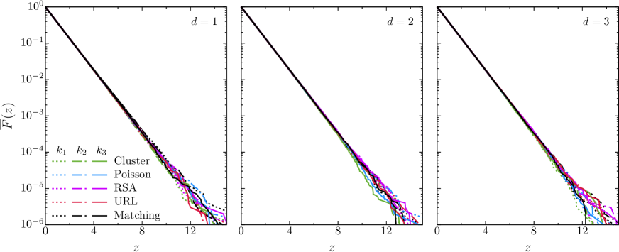
Figure 2: Empirical complementary distribution function $\overline{F}$ of the scaled scattering intensity $\mathcal{S}(k)/\overline{\mathcal{S}}(k)$.

According to Proposition 5.4 and the scaling $\mathcal{S}(k)\mapsto\mathcal{S}(k)/\overline{\mathcal{S}}(k)$, the function $\overline{F}$ should hopefully be close to the reciprocal exponential function, which is the complementary distribution function of a unit rate exponential distribution. In this respect, a look at Fig. 2 is illustrative. On a logarithmic scale, this figure displays the empiricial complementary cumulative distribution function $\overline{F}$ of the scattering intensity for the cases $d=1$ (left), $d=2$ (middle) and $d=3$ (right). Due to the scaling, all curves of $\overline{F}$ collapse, irrespective of the special choice of the model or of the wave vector. Moreover, in each of the cases considered $\overline{F}$ agrees with an exponential function to surprisingly high accuracy. Such a close agreement has also been observed for each of many other wave vectors that have been considered. Notice that the small fluctuations of $\overline{F}(z)$ at the order of $10^{-6}$, which are visible only for large values of $\mathcal{S}(k)/\overline{\mathcal{S}}(k)$, are in accord with purely statistical fluctuations for our $10^{6}$ samples, i.e., we do not observe systematic deviations from an exponential distribution.

Last but not least, according to our findings there is only a weak correlation of $\mathcal{S}(k)$ for different wave vectors $k$. Even for neighboring wave vectors that are close to the origin in Fourier space, the correlation coefficient is throughout smaller than 0.02. This observation is in excellent agreement with Proposition 5.4.

6 Maximum likelihood estimation

In this section, we adopt an asymptotic setting that suggests itself in view of Proposition 5.4. In this setting the background of point processes is not important any more, and our starting point is the multivariate asymptotic distribution of scattering intensities, as provided by Proposition 5.4. In this asymptotic setting, we can define maximum likelihood estimators of a parameterized structure factor. More specifically, we employ the expansion (2.9) of $S(k)$ as $k\to 0$. While a limitation to this expansion entails an additional element of approximation, (2.9) holds in the same limit of large system sizes in the sense that in this limit small wave vectors become accessible.

To proceed, take $n$ wave vectors $k_{1},\ldots,k_{n}\in{\mathbb{R}}^{[d]}\setminus\{0\}$ and put $\kappa_{j}:=\|k_{j}\|^{2}$, $j\in[n]$. In an abuse of the hitherto existing meaning, let $X_{1},\ldots,X_{n}$ be independent exponentially distributed random variables, where $\mathbb{E}(X_{j})=s+t\kappa_{j}$, $j\in[n]$. Here, $s\geq 0$ and $t\in{\mathbb{R}}$ are unknown parameters that have to be estimated based on realizations $x_{1},\ldots,x_{n}$ of $X_{1},\ldots,X_{n}$. Note that this statistical problem is of interest for its own sake. More formally, the underlying parameter space is

$$\Theta :=\{(s,t)\in{\mathbb{R}}^{2}:s\geq 0,s+t\kappa_{1}>0,\ldots,s+t\kappa_{n}>0\}$$

$$=\bigg{\{}(s,t)\in{\mathbb{R}}^{2}:s\geq 0,t>-\frac{s}{\max(\kappa_{1},\ldots,\kappa_{n})}\bigg{\}},$$

which defines a cone in the $(s,t)$-plane. For $(s,t)\in\Theta$, let $\mathbb{P}_{s,t}$ denote a probability measure that governs the above random variables. The associated expectation and variance operator are denoted by $\mathbb{E}_{s,t}$ and $\operatorname{{\mathbb{V}ar}}_{s,t}$, respectively. For convenience this notation suppresses the dependence both on $n$ and on $k_{1},\ldots,k_{n}$. Our null hypothesis $H_{0}$ (say) is hyperuniformity, which in view of the asymptotic setting and the constraint imposed by (2.9), is characterized by the subset $\Theta_{0}:=\{(s,t)\in\Theta:s=0\}$ of $\Theta$.

Under $\mathbb{P}_{s,t}$ the density of $X_{j}$, $j\in[n]$, is given by

$$y\mapsto\frac{1}{s+t\kappa_{j}}\exp\left(-\frac{y}{s+t\kappa_{j}}\right),\quad y\geq 0.$$

The log-likelihood function corresponding to observed positive values $x_{1},\ldots,x_{n}$ is

$$\mathcal{L}(x_{1},\ldots,x_{n};s,t)=\sum_{j=1}^{n}\Big{[}-\log(s+t\kappa_{j})-\frac{x_{j}}{s+t\kappa_{j}}\Big{]}.$$ (6.1)

We first consider maximum likelihood estimation of $t$ under the null hypothesis $H_{0}$.

6.1 Estimation under $H_{0}$

Under $\mathbb{P}_{0,t}$, that is, under the constraint $s=0$ imposed by $H_{0}$, the log-likelihood function simplifies to

$$\mathcal{L}(x_{1},\dots,x_{n};0,t)=-n\log t-\frac{1}{t}\sum_{j=1}^{n}\frac{x_{j}}{\kappa_{j}}-\sum_{j=1}^{n}\log\kappa_{j}.$$

The first two derivatives read

$$\frac{\partial\mathcal{L}}{\partial t}(x_{1},\dots,x_{n};0,t) =-\frac{n}{t}+\frac{1}{t^{2}}\sum_{j=1}^{n}\frac{x_{j}}{\kappa_{j}},$$

$$\frac{\partial^{2}\mathcal{L}}{\partial t^{2}}(x_{1},\dots,x_{n};0,t) =\frac{n}{t^{2}}-\frac{2}{t^{3}}\sum_{j=1}^{n}\frac{x_{j}}{\kappa_{j}}.$$

If we define a function $h_{0}$ on $(0,\infty)^{n}$ by

$$h_{0}(x_{1},\ldots,x_{n}) :=\sup\{\mathcal{L}(x_{1},\ldots,x_{n};0,t):(0,t)\in\Theta\},$$ (6.2)

the maximum likelihood (ML) estimate $\widehat{t}_{0}\equiv\widehat{t}_{0}(x_{1},\ldots,x_{n})$ of $t$ based on $x_{1},\ldots,x_{n}$ is uniquely determined by $\mathcal{L}(x_{1},\ldots,x_{n};0,\widehat{t}_{0})=h_{0}(x_{1},\ldots,x_{n})$, and it takes the form

$$\widehat{t}_{0}(x_{1},\ldots,x_{n})=\frac{1}{n}\sum_{j=1}^{n}\frac{x_{j}}{\kappa_{j}}.$$

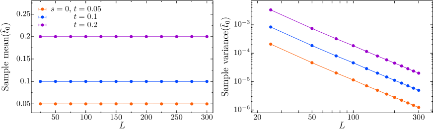
Figure 3: Unbiasedness and consistency of $\widehat{t}_{0}$ are demonstrated by plots of the sample mean value (left) and variance (right) as functions of the linear system size $L$.

Recall that the gamma distribution with shape parameter $\alpha$ and scale parameter $\beta$ has density

$$y\mapsto{\mathbf{1}}\{y\geq 0\}\frac{\beta^{\alpha}y^{\alpha-1}{\mathrm{e}}^{-\beta x}}{\Gamma(\alpha)}.$$

Under $\mathbb{P}_{0,t}$, $\widehat{t}_{n}(X_{1},\ldots,X_{n})$ is the average of $n$ independent exponential random variables with mean value $t$. By a standard convolution property of the gamma distribution, $\widehat{t}_{n}(X_{1},\ldots,X_{n})$ follows a gamma distribution with shape parameter $\alpha=n$ and scale parameter $\beta=n/t$. Since

$$\mathbb{E}_{0,t}\big{(}\widehat{t}_{n}(X_{1},\ldots,X_{n})\big{)}=\frac{\alpha}{\beta}=t,\qquad\operatorname{{\mathbb{V}ar}}_{0,t}\big{(}\widehat{t}_{n}(X_{1},\ldots,X_{n})\big{)}=\frac{\alpha}{\beta^{2}}=\frac{t^{2}}{n},$$

the estimator $\widehat{t}_{0}(X_{1},\ldots,X_{n})$ is unbiased for $t$, and the sequence $(\widehat{t}_{0}(X_{1},\ldots,X_{n}))$ is consistent. In the following we often abuse notation by writing $\widehat{t}_{0}$ instead of $\widehat{t}_{0}(X_{1},\ldots,X_{n})$. The meaning will be clear from the context. A similar notation will be used for two other estimators to be introduced below.

Figure 3 illustrates the properties of unbiasedness and consistency of $\widehat{t}_{0}$ for three different values of $t$. The left hand figure displays arithmetic means as estimators $\widehat{\mathbb{E}}(\widehat{t}_{0})$ of the expectation, and the right hand figure shows the sample variance as estimators $\widehat{\operatorname{{\mathbb{V}ar}}}(\widehat{t}_{0})$ of the variance. For each choice of the parameters $t$ and $L$, the estimates are based on $10^{6}$ independent realizations of $(X_{1},\ldots,X_{n})$. For the case $s=0$ and $L=100$, Figure 4 exhibits the corresponding histograms of the distribution of $\widehat{t}_{0}$, which are in excellent agreement with fitted gamma distributions. Usually, a histogram uses columns that mark as areas the frequency corresponding to the range of their base. In our case, the intervals forming the bases are of equal length, and instead of columns we preferred to use bullets. The horizontal coordinate of a bullet is the midpoint of its base. The height of a bullet is the relative frequency of the data falling into the corresponding base, divided by length of the bases, and is thus an estimate of the density of $\widehat{t}_{0}$ at the midpoint of the base. Mutatis mutandis, these remarks refer to each subsequent figure that displays a histogram.

In each of our simulations, we choose wave vectors from the reciprocal lattice that corresponds to the periodic simulation box, which is defined as

$$\{k\in{\mathbb{R}}^{[d]}\setminus\{0\}:\|k\|<b\text{ and }k_{j}=2\pi n_{j}/L\text{ with }n_{j}\in{\mathbb{Z}}\text{ for each }j\in[d]\}.$$ (6.3)

Here we use $d=2$ and $b=0.75$. Other choices of $d$ and $b$ yield essentially the same results. Only the speed of convergence differs, as expected.

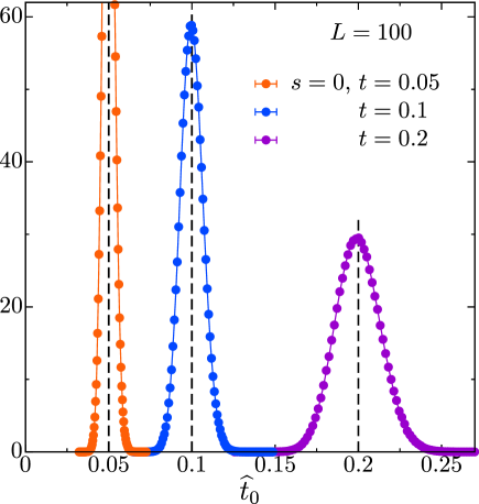
Figure 4: Histograms of the continuous part of the distribution of $\widehat{t}_{0}$ (bullets) and densities of gamma distributions with the same expectation and variance (solid lines).

6.2 Estimation in the full parameter space

When $s$ and $t$ are allowed to vary freely in $\Theta$, we do not know how to maximize (6.1) explicitly. However, since $\Theta$ is a cone in the $(s,t)$-plane, the problem of maximizing a function of two variables can be reduced to a univariate optimization problem. Dropping the arguments $x_{1},\ldots,x_{n}$ in the notation of the log-likelihood function, we have for $(s,t)\in\Theta$ and $\delta>0$

$$\mathcal{L}(\delta s,\delta t)=\mathcal{L}(s,t)-n\log\delta+\left(1-\frac{1}{\delta}\right)\sum_{j=1}^{n}\frac{x_{j}}{s+t\kappa_{j}}.$$

Notice that

$$\frac{{\text{d}}}{{\text{d}}\delta}\mathcal{L}(\delta s,\delta t)=-\frac{n}{\delta}+\frac{1}{\delta^{2}}\sum_{j=1}^{n}\frac{x_{j}}{s+t\kappa_{j}}.$$

This derivative vanishes if, and only if,

$$\delta=\delta_{0}:=\frac{1}{n}\sum_{j=1}^{n}\frac{x_{j}}{s+t\kappa_{j}}.$$

Since $\frac{{\text{d}}}{{\text{d}}\delta}\mathcal{L}(\delta s,\delta t)$ is positive if $\delta<\delta_{0}$ and negative if $\delta>\delta_{0}$, the function $(0,\infty)\ni\delta\mapsto\mathcal{L}(\delta s,\delta t)$ has a unique maximum, which is attained at $\delta=\delta_{0}$. Plugging $\delta_{0}$ into the definition of $\mathcal{L}(\delta s,\delta t)$ and setting $s=\cos\vartheta$, $t=\sin\vartheta$ gives

$$\mathcal{L}^{*}(\vartheta) :=\max_{\delta>0}\mathcal{L}(\delta\cos\vartheta,\delta\sin\vartheta)$$

$$=\mathcal{L}(\cos\vartheta,\sin\vartheta)-1-n\log\left(\sum_{j=1}^{n}\frac{x_{j}}{\cos\vartheta+\kappa_{j}\sin\vartheta}\right)+\sum_{j=1}^{n}\frac{x_{j}}{\cos\vartheta+\kappa_{j}\sin\vartheta}.$$

Using $\log(ab)=\log a+\log b$ if $a,b>0$, some algebra yields

$$\mathcal{L}^{*}(\vartheta)=-\sum_{j=1}^{n}\log\big{(}1+\kappa_{j}\tan\vartheta\big{)}-1-n\log\left(\sum_{j=1}^{n}\frac{x_{j}}{1+\kappa_{j}\tan\vartheta}\right)$$

It remains to maximize $\mathcal{L}^{*}(\vartheta)$ as a function of $\vartheta$, where $\vartheta$ runs from $\vartheta_{0}$ to $\pi/2$ and $\tan\vartheta_{0}=-1/\max(\kappa_{1},\ldots,\kappa_{n})$. Putting $y:=\cot\vartheta$ and $\widetilde{\mathcal{L}}(y):=\mathcal{L}^{*}(\vartheta)$, the task is to maximize the function

$$\widetilde{\mathcal{L}}(y)=-\sum_{j=1}^{n}\log\left(1+\frac{\kappa_{j}}{y}\right)-1-n\log\left(\sum_{j=1}^{n}\frac{x_{j}}{1+\kappa_{j}/y}\right),$$

where $y\in\big{(}\-\infty,-\min(\kappa_{1},\ldots,\kappa_{n})\big{)}\cup(0,\infty)$. The maximum of $\widetilde{\mathcal{L}}$ can be attained in the limit $y\downarrow 0$. The next result provides some information on the function $\widetilde{\mathcal{L}}$.

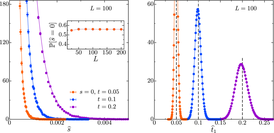
Figure 5: Histograms of the continuous parts of the distribution of $\widehat{s}$ and $\widehat{t}_{1}$ (bullets) and densities of gamma distributions with the same expectation and variance (solid lines). The inset shows the size of the atom of $\widehat{s}$ as a function of $L$.

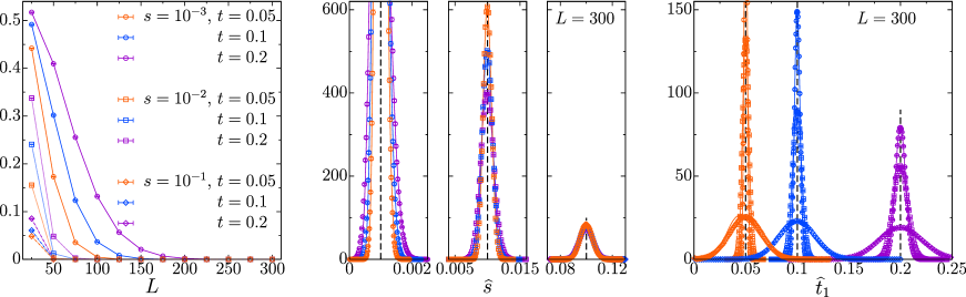
Figure 6: The non-hyperuniform case: (left) the size of the atom of $\widehat{s}$; (center and right) histograms of the distributions of $\widehat{s}$ and $\widehat{t}_{1}$ (bullets) and densities of gamma distributions with the same expectation and variance (solid lines).

Lemma 6.1.

Let $y_{0}:=-\min(\kappa_{1},\ldots,\kappa_{n})$. We have

1. $\displaystyle{\lim_{y\downarrow-\infty}\widetilde{\mathcal{L}}(y)=-1-n\log\left(\sum_{j=1}^{n}x_{j}\right)}$,

2. $\displaystyle{\lim_{y\uparrow y_{0}}\widetilde{\mathcal{L}}(y)=-\infty}$,

3. $\displaystyle{\lim_{y\downarrow 0}\widetilde{\mathcal{L}}(y)=-\sum_{j=1}^{n}\log\kappa_{j}-1-n\log\left(\sum_{j=1}^{n}\frac{x_{j}}{\kappa_{j}}\right)}$,

4. $\displaystyle{\lim_{y\uparrow\infty}\widetilde{\mathcal{L}}(y)=-1-n\log\left(\sum_{j=1}^{n}x_{j}\right)}$.

Proof.

a) and d) follow readily from the definition of $\widetilde{\mathcal{L}}$. To prove b), let $\kappa_{1}\leq\ldots\leq\kappa_{n}$ without loss of generality. Moreover, assume that $\kappa_{1}=\ldots=\kappa_{\ell}<\kappa_{\ell+1}$ for some $\ell\in\{1,\ldots,n-1\}$. Furthermore, put $t:=1+\kappa_{1}/y$. Notice that $y\uparrow y_{0}$ is equivalent to $t\downarrow 0$. The definition of $\ell$ and $t$ give

$$\widetilde{\mathcal{L}}(y) = -\ell\log t-\sum_{j=\ell+1}^{n}\log\left(1+\frac{\kappa_{j}}{y}\right)-1-n\log\left(\frac{1}{t}\left(\sum_{j=1}^{\ell}x_{j}+t\sum_{j=\ell+1}^{n}\frac{x_{j}}{1+\kappa_{j}/y}\right)\right)$$

$$= (n-\ell)\log t-\sum_{j=\ell+1}^{n}\log\left((1+\frac{\kappa_{j}}{y}\right)-1-n\log\left(\sum_{j=1}^{\ell}x_{j}+t\sum_{j=\ell+1}^{n}\frac{x_{j}}{1+\kappa_{j}/y}\right)$$

$$= (n-\ell)\log t+O(1),$$

where $O(1)$ denotes a term that is bounded as $t\to 0$. Since $\ell<n$, assertion c) follows. If $y>0$ then – using $\log(ab)=\log a+\log b$ if $a,b>0$ – we have

$$\widetilde{\mathcal{L}}(y)=-\sum_{j=1}^{n}\log\left(\kappa_{j}+y\right)-1-n\log\left(\sum_{j=1}^{n}\frac{x_{j}}{y+\kappa_{j}}\right),$$

and the proof is completed. ∎

Similarly as in (6.2) we define a function $h_{1}$ on $(0,\infty)^{n}$ by

$$h_{1}(x_{1},\ldots,x_{n}) :=\sup\{\mathcal{L}(x_{1},\ldots,x_{n};s,t):(s,t)\in\Theta\}.$$ (6.4)

Given $(x_{1},\ldots,x_{n})$, let $\widehat{\Theta}(x_{1},\ldots,x_{n})$ denote the set of all $(s^{\prime},t^{\prime})\in\Theta$ such that

$$\mathcal{L}(x_{1},\ldots,x_{n};s^{\prime},t^{\prime})=h_{1}(x_{1},\ldots,x_{n}).$$

By Lemma 6.1, the set $\widehat{\Theta}(x_{1},\ldots,x_{n})$ is non-empty.

We do not have further mathematical results on the behavior of the function $\widetilde{\mathcal{L}}$. However, there ist strong heuristic evidence that there ist only one maximizer $y\in[0,\infty)$ of $\widetilde{\mathcal{L}}$. Moreover, this maximizer is $0$ if the right hand derivative of $\widetilde{\mathcal{L}}$ at $0$ is negative, and it is positive if this right hand derivative ist positive. Notice that the derivative of $\widetilde{\mathcal{L}}$ is given by

$$\widetilde{\mathcal{L}}^{\prime}(y)=-\sum_{j=1}^{n}\frac{1}{\kappa_{j}+y}+n\,\frac{\sum_{j=1}^{n}\frac{x_{j}}{(y+\kappa_{j})^{2}}}{\sum_{j=1}^{n}\frac{x_{j}}{y+\kappa_{j}}}.$$

Hence,

$$\widetilde{\mathcal{L}}^{\prime}(0):=\lim_{y\downarrow 0}\widetilde{\mathcal{L}}^{\prime}(y)=-\sum_{j=1}^{n}\frac{1}{\kappa_{j}}+n\,\frac{\sum_{j=1}^{n}\frac{x_{j}}{\kappa_{j}^{2}}}{\sum_{j=1}^{n}\frac{x_{j}}{\kappa_{j}}},$$

and we have

$$\widetilde{\mathcal{L}}^{\prime}(0)<0\Longleftrightarrow\sum_{j=1}^{n}\frac{x_{j}}{\kappa_{j}}\left(\frac{1}{n}\sum_{i=1}^{n}\frac{1}{\kappa_{i}}-\frac{1}{\kappa_{j}}\right)>0.$$

Remark 6.2.

Let $(x_{1},\ldots,x_{n})\in(0,\infty)^{n}$. Our numerical analysis strongly suggests that

$$\widehat{\Theta}(x_{1},\ldots,x_{n})=\{(\widehat{s}(x_{1},\ldots,x_{n}),\widehat{t}_{1}(x_{1},\ldots,x_{n}))\}$$ (6.5)

for some (uniqely determined) maximizing pair $(\widehat{s}(x_{1},\ldots,x_{n}),\widehat{t}_{1}(x_{1},\ldots,x_{n}))\in\Theta$. This claim is also supported by Lemma 6.1. Whenever we use the notation $\widehat{s}(\cdot)$ and $\widehat{t}_{1}(\cdot)$ we assume (6.5), at least implicitly.

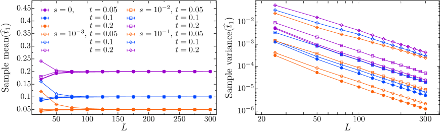
Figure 7: Asymptotic unbiasedness and consistency of $\widehat{t}_{1}$ are illustrated by plots of the sample mean value (left) and variance (right) as functions of the linear system size $L$.

Before discussing the findings of our simulations, we provide two useful invariance properties.

Lemma 6.3.

Let $t>0$. Then

$$\mathbb{P}_{0,t}(h_{1}(X_{1},\ldots,X_{n})-h_{0}(X_{1},\ldots,X_{n})\in\cdot)=\mathbb{P}_{0,1}(h_{1}(X_{1},\ldots,X_{n})-h_{0}(X_{1},\ldots,X_{n})\in\cdot).$$

Proof.

The parameter space $\Theta$ is invariant under scaling with positive constants. Moreover, the log-likelihood function is essentially scale free, since

$$\mathcal{L}(rx_{1},\ldots,rx_{n};rs,rt)=\mathcal{L}(x_{1},\ldots,x_{n};s,t)-n\log r,$$

for each $r>0$, each $(s,t)\in\Theta$ and each $(x_{1},\ldots,x_{n})\in(0,\infty)^{n}$. It follows that

$$h_{1}(rx_{1},\ldots,rx_{n})-h_{0}(rx_{1},\ldots,rx_{n})=h_{1}(x_{1},\ldots,x_{n})-h_{0}(x_{1},\ldots,x_{n}).$$

Putting $r:=t^{-1}$, and using the distributional identity

$$\mathbb{P}_{0,t}\big{(}(t^{-1}X_{1},\ldots,t^{-1}X_{n})\in\cdot\big{)}=\mathbb{P}_{0,1}\big{(}(X_{1},\ldots,X_{n})\in\cdot\big{)},$$

the result follows. ∎

If assumption (6.5) holds, then the next corollary implies

$$\mathbb{P}_{0,t}\big{(}\widehat{s}(X_{1},\ldots,X_{n})=0\big{)}=\mathbb{P}_{0,1}\big{(}\widehat{s}(X_{1},\ldots,X_{n})=0\big{)},\quad t>0.$$

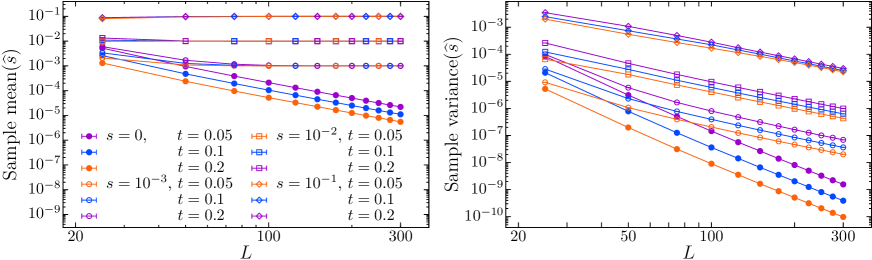
Figure 8: Asymptotic unbiasedness and consistency of $\widehat{s}$ are demonstrated by plots of the mean value (left) and variance (right) as functions of $L$.

Corollary 6.4.

Let $t>0$. Then

$$\mathbb{P}_{0,t}\big{(}\widehat{\Theta}(X_{1},\ldots,X_{n})\cap\Theta_{0}=\emptyset\big{)}=\mathbb{P}_{0,1}\big{(}\widehat{\Theta}(X_{1},\ldots,X_{n})\cap\Theta_{0}=\emptyset\big{)}.$$

Proof.

Let $(x_{1},\ldots,x_{n})\in(0,\infty)^{n}$. Assume that $\widehat{\Theta}(x_{1},\ldots,x_{n})\cap\Theta_{0}\neq\emptyset$. We then obtain straightly from the definitions that $h_{0}(x_{1},\ldots,x_{n})=h_{1}(x_{1},\ldots,x_{n})$. Assume conversely that the latter identity holds. As we have already seen, there exists $\widehat{t}_{0}>0$ such that $\mathcal{L}(x_{1},\ldots,x_{n};0,\widehat{t}_{0})=h_{0}(x_{1},\ldots,x_{n})$. Therefore, $(0,\widehat{t}_{0})\in\widehat{\Theta}(x_{1},\ldots,x_{n})$ and hence $\widehat{\Theta}(x_{1},\ldots,x_{n})\cap\Theta_{0}\neq\emptyset$. The assertion thus follows from Lemma 6.3. ∎

We numerically optimize $\mathcal{L}(x_{1},\ldots,x_{n};s,t)$ with machine precision, i.e., a tolerance of $10^{-14}$. Such a high accuracy is in fact necessary to reliably study the $\mathbb{P}_{s,t}$-distribution of $\widehat{s}(X_{1},\ldots,X_{n})$, since the density of the continuous part diverges as $s\to 0$.

Using the same wave vectors as for Figs. 3 and 4, we repeat the optimization for $10^{6}$ independent simulations of the vector of $(X_{1},\ldots,X_{n})$ for each choice of $s$, $t$, and $L$. We then approximate the densities of $\widehat{s}(X_{1},\ldots,X_{n})$ and $\widehat{t}_{1}(X_{1},\ldots,X_{n})$ with histograms of the simulation results, see Figs. 5 and 6 for simulations with $s=0$ and $s>0$, respectively. The inset in Fig. 5 and the left panel in Fig. 6 show the stabilization of the size of the atom. Asymptotic unbiasedness and consistency are illustrated in Figs. 7 and 8.

Our simulations strongly suggest the following asymptotic behavior of our estimators:

• The estimators are consistent and asymptotically unbiased.

• The asymptotic distribution (as $L\to\infty$) of $\widehat{s}(X_{1},\ldots,X_{n})$ has an atom at the origin. The atom size $\mathbb{P}_{s,t}(\widehat{s}(X_{1},\ldots,X_{n})=0)$ converges to zero if $s>0$ and to a constant that is independent of $t$, otherwise. The latter independence follows from Corollary 6.4.

• As $L\to\infty$, the continuous part of the distribution of both $\widehat{s}(X_{1},\ldots,X_{n})$ and $\widehat{t}_{1}(X_{1},\ldots,X_{n})$ converges to a gamma distribution. For $s=0$, the distributions of $\widehat{s}(X_{1},\ldots,X_{n})$ and $\widehat{t}_{1}(X_{1},\ldots,X_{n})$ are well approximated by a gamma distribution already at relatively small system sizes.

7 Likelihood ratio test for hyperuniformity

In this section we adopt the setting of Section 6. We define the test statistic

$$T(x_{1},\dots,x_{n}):=2[h_{1}(x_{1},\dots,x_{n})-h_{0}(x_{1},\dots,x_{n})],\quad(x_{1},\ldots,x_{n})\in(0,\infty)^{n},$$ (7.1)

where $h_{0}$ and $h_{1}$ are given by (6.2) and (6.4), respectively. By definition $T$ is nonnegative. Under our hypothesis (6.5) we have $T(x_{1},\ldots,x_{n})=0$ if, and only if, $\widehat{s}(x_{1},\ldots,x_{n})=0$. Hence the $\mathbb{P}_{s,t}$-atom of $\widehat{s}(X_{1},\ldots,X_{n})$ is inherited by $T(X_{1},\ldots,X_{n})$.

Based on our simulation results displayed in Fig. 9, we conjecture that, as $n\to\infty$, the limit distribution of $T$ under $H_{0}$ is a mixture of an atom at $0$ and a gamma distribution with parameters $\alpha=k/2$ and $\beta=1/2$, where $k$ is slightly smaller than $1$. For $k=1$ the latter would be a $\chi^{2}$-distribution with one degree of freedom. In our case, we still refer to a $\chi^{2}$-distribution with a fractional parameter $k$. Importantly, this observation holds to a good approximation even for small system sizes. In particular, it implies that the asymptotic distribution of $T$ does not depend on $t$. In fact, this latter statement follows directly from Lemma 6.3. The existence of an universal ($t$-independent) explicit limit distribution of $T$ is key for our test on hyperuniformity.

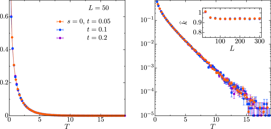
Figure 9: Histogram of the density of the continuous part of the distribution of $T$ in an asymptotic framework, i.e., for exponentially distributed and independent values of $S(k)$ with $s=0$.

Under $H_{1}$, the distribution of $T$ is asymptotically (for $n\to\infty$) well described by a gamma distribution with effectively one parameter (i.e., a scatter plot of $\alpha$ and $\beta$ collapses to a single curve); see Fig. 10, where we use the same simulation parameters as in Sec. 6 for additional values of $s$, $t$, and $L$.

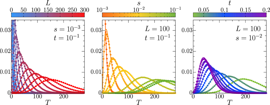
Figure 10: Histogram of the density of the continuous part of the distribution of $T$ in an asymptotic framework, but now with different values of $s$, $t$, and $L$.

8 Testing hyperuniformity in an example

Finally, we demonstrate the practical relevance and remarkable sensitivity of our test by applying it to model (v) of matched points in Sec. 5. The advantages of the model are that it exhibits correlations, nevertheless it is known to be hyperuniform [32]. Importantly, large samples can be easily simulated. Moreover, the parameter $t$ can be easily adjusted by varying the intensity $\alpha$. As before, we simulate two-dimensional models, but in principle the results are applicable in any dimension. A further advantage of model (v) is that the parameter $t$ can readily be adjusted by varying the intensity $\alpha$.

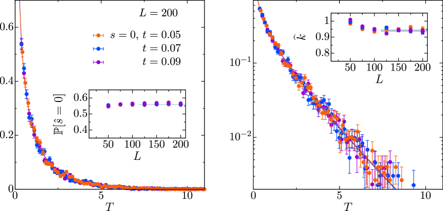
Figure 11: Histogram of the density of the continuous part of the distribution of $T$ for matched point patterns.

We first demonstrate that the approximations in the previous sections apply with high accuracy to our actual point patterns with system sizes that are commonly used in applications; see [39] and references therein. Figure 11 shows the empirical probability density of $T$ for different values of $t$. All curves collapse on the predicted $\chi^{2}$-distributions within the statistical error bars. The insets of Fig. 11 show the two parameters of the distribution, i.e., the size of the atom and the ‘fractional degree of freedom’, as a function of $L$. The data for our point patterns (bullets) is good agreement with the results from the asymptotic setting (represented by horizontal lines). The specific simulation parameters are as follows. We adapt the maximum length of the wave vectors to $\alpha$, i.e., to the range for which the parabolic approximation holds with high precision. More specifically, the parameter $b$ in (6.3) is set to 0.50 for $\alpha=3.0$ (i.e., $t\approx 0.05$), 0.40 for $\alpha=2.5$ (i.e., $t\approx 0.07$), and 0.33 for $\alpha=2.0$ (i.e., $t\approx 0.09$). Note that these are simple ad-hoc values of $b$. Our results do not sensitively depend on $b$. We also adjust the number of independent samples for each linear system size: 500000 for $L=50$, 200000 for $L=75$, 100000 for $L=100$, 50000 for $L=125$, 40000 for $L=150$, 30000 for $L=175$, and 20000 for $L=200$.

We use independent thinning to smoothly vary the value of $S(0)$. Given $p\in[0,1]$ and a stationary point process $\eta$, the $p$-thinning $\eta_{p}$ of $\eta$ is obtained by keeping the points of $\eta$ independently of each other with probability $p$; see [34, Section 5.3]. A simple computation shows that the intensity $\gamma_{p}$ and the covariance measure $\beta^{!}_{2,p}$ of $\eta_{p}$ are given by $\gamma_{p}=p\gamma$ and $\beta^{!}_{2,p}=p^{2}\beta^{!}_{2}$, respectively. Hence, if the structure factor can be defined by (2.8), then

$$S_{p}(k)=1-p+pS(k),\quad k\in{\mathbb{R}}^{d},$$ (8.1)

where $S_{p}$ is the structure factor of $\eta_{p}$; see also [28]. This fact remains true under assumptions (2.10) and (2.12). For the matching process none of these definitions apply. In such cases we still assume that $S-1$ is a homogeneous function of $\gamma^{-1}\beta^{!}_{2}$, whenever $S$ is well-defined in terms of $\beta^{!}_{2}$. This assumption means that the function $\Phi$ mapping the positive semi-definite signed measure $\nu=\gamma^{-1}\beta^{!}_{2}$ to $S-1$ satisfies $\Phi(r\nu)=r\Phi(\nu)$ for all $r\geq 0$, enforcing (8.1).

Using thinning we can vary the value of $s$, i.e., of the structure factor at the origin. We started with $s=10^{-4}$, which is an order of magnitude smaller than typical non-hyperuniform models [39, 31], and we then increased the value of $s$ up to $0.1$. For each pair of $s$ and $L$, we simulated 5000 independent point patterns.

The entries of Table 1 display the fraction of simulated samples for which the null hypothesis is rejected, rounded to two decimal places. These values thus convey an impression of the power of the test. An asterisk denotes rejection for each sample and thus power one. The nominal significance level is $0.05$. Here we set $\alpha=3.0$, which corresponds to $t\approx 0.05$. Based on the simulation results in Sec. 6.1 for $t=0.05$ and $L=300$, we assume for the distribution of $T$ the size of the atom to be about 0.559 and the fractional degree of freedom to be about 0.944 for the continuous part. Here we use $b=0.75$ as the maximum length of a wave vector in (6.3). We found that slightly larger values of $b$ still keep the significance level, and that they raise the power of the test. However, $b$ must not be taken too large, since otherwise the parabolic approximation would be violated.

The first line of Table 1 illustrates that, within statistical fluctuations, the test maintains the nominal significance level. For each value $s>0$, the power quickly increases with increasing system size $L$ or value of $s$, i.e., of the structure factor at the origin. For a single sample with only 2500 points (i.e., $L=50$), almost each sample with $s>10^{-2}$ is rejected. Even for $s=10^{-4}$, which is often considered to be a borderline case for physical applications [39, 31], our test rejects more than $90\%$ of the samples with $L=300$, i.e., 90000 points.

	50	100	150	200	250	300	400
0.0	0.05	0.06	0.06	0.05	0.05	0.06	0.05
0.0001	0.08	0.20	0.40	0.64	0.83	0.93	1.00
0.00025	0.12	0.41	0.77	0.95	0.99	1.00	$\ast$
0.0005	0.21	0.70	0.95	1.00	$\ast$	$\ast$	$\ast$
0.00075	0.27	0.84	0.99	$\ast$	$\ast$	$\ast$	$\ast$
0.001	0.35	0.93	1.00	$\ast$	$\ast$	$\ast$	$\ast$
0.0025	0.68	1.00	$\ast$	$\ast$	$\ast$	$\ast$	$\ast$
0.005	0.88	$\ast$	$\ast$	$\ast$	$\ast$	$\ast$	$\ast$
0.0075	0.95	$\ast$	$\ast$	$\ast$	$\ast$	$\ast$	$\ast$
0.01	0.97	$\ast$	$\ast$	$\ast$	$\ast$	$\ast$	$\ast$
0.025	1.00	$\ast$	$\ast$	$\ast$	$\ast$	$\ast$	$\ast$
0.05	1.00	$\ast$	$\ast$	$\ast$	$\ast$	$\ast$	$\ast$
0.075	1.00	$\ast$	$\ast$	$\ast$	$\ast$	$\ast$	$\ast$
0.1	1.00	$\ast$	$\ast$	$\ast$	$\ast$	$\ast$	$\ast$

Table 1: Power of the novel test for hyperuniformity for a range of values of $s$ and $L$. Each test is applied to only a single sample of the thinned model (v).

9 Final remarks

Our test hinges on essentially three approximations, each of which holding in the same (thermodynamic) limit, i.e., for large system sizes. In this limit, the scattering intensity becomes both exponentially distributed and independent for different wave vectors. In the same limit, the number of available wave vectors in a neighborhood around the origin diverges, and the distribution of the test statistic converges to a specific mixture of an atom at $0$ and a gamma distribution. Future work might show that the latter convergence may also be obtained even for a finite (but not too small) sample size, in the limit of a large number of samples. Finally, in the limit of large system sizes, even the parabolic approximation (2.9) holds in the following sense. As the system size gets larger, smaller wave vectors become available, and hence the parabolic approximation improves. Strictly speaking, the range of wave numbers for which the fit is applied has to be adapted in the limit of large sample sizes. Such an adaptation, however, does not raise practical problems.

It is an interesting task to find further rigorous examples of point processes that satisfy our crucial assumption (5.2); see Remark 5.3. Future work might also yield more evidence regarding the asymptotic behavior of the ML-estimator and the test statistic, obtained from simulations. We are not aware of corresponding results in the literature that could be applied to a sequence of independent exponential random variables with varying means that depend on constrained parameters.

We have applied our test in extensive simulations to thinnings of the matching process from [32]. Preliminary results for other point processes are equally promising. Finally, we will provide an open-source python package, so that anyone can conveniently apply the test to their data sets. Any feedback is very much welcome.

Acknowledgements: This research was supported by the Deutsche Forschungsgemeinschaft (DFG, German Research Foundation) as part of the DFG priority program ‘Random Geometric Systems’ SPP 2265) under grants LA 965/11-1, LO 418/25-1, ME 1361/16-1, and WI 5527/1-1, and by the Volkswagenstiftung via the ‘Experiment’ Project ‘Finite Projective Geometry’.

References

• [1] Atkinson, S., Zhang, G., Hopkins, A. B. and Torquato, S. (2016). Critical slowing down and hyperuniformity on approach to jamming. Phys. Rev. E 94, 012902-1–14.
• [2] Berg, C.  and Forst, G. (1975). Potential Theory on Locally Compact Abelian Groups. Springer, New-York.
• [3] Billingsley, P. (1995). Probability and Measure. Third Edition, Wiley, New York.
• [4] Biscio, C.A.N. and Waagepetersen, R. (2019). A general central limit theorem and a subsampling variance estimator for $\alpha$-mixing point processes. Scand. J. Stat. 46, 1168–1190.
• [5] Brémaud, P. (2020). Point Process Calculus in Time and Space. Springer, Cham.
• [6] Brillinger, D.R. (2012). The spectral analysis of stationary interval functions. In: Selected Works of David Brillinger (pp. 25-55). Springer, New York.
• [7] Camilier, I. and Decreusefond, L. (2010). Quasi-invariance and integration by parts for determinantal and permanental processes. J. Funct. Anal. 259, 268–300.
• [8] Chatterjee, S. (2019). Rigidity of the three-dimensional hierarchical Coulomb gas. Probab. Theory Related Fields 175, 1123–1176.
• [9] Chen, D., Zheng, Y., Liu, L., Zhang, G., Chen, M., Jiao, Y., and Zhuang, H. (2021). Stone–Wales defects preserve hyperuniformity in amorphous two-dimensional networks. Proc. Natl. Acad. Sci. U.S.A. 118, e2016862118–1–9.
• [10] Chiu, S.N., Stoyan, D., Kendall, W.S. and Mecke, J. (2013). Stochastic Geometry and its Applications. 3rd edn. Wiley, Chichester.
• [11] Daley, D.J. and Vere-Jones, D. (2003/2008). An Introduction to the Theory of Point Processes. Volume I: Elementary Theory and Methods, Volume II: General Theory and Structure. Second Editionn. Springer, New York.
• [12] Dreyfus, R., Xu, Y., Still, T., Hough, L. A., Yodh, A. G., and Torquato, S. (2015). Diagnosing hyperuniformity in two-dimensional, disordered, jammed packings of soft spheres. Phys. Rev. E 91, 012302.
• [13] Gabrielli, A., Jancovici, B., Joyce, M., Lebowitz, J. L., Pietronero, L. and Labini, F.S. (2003). Generation of primordial cosmological perturbations from statistical mechanical models. Phys. Rev. D, 67, 043506.
• [14] Ghosh, S. and Lebowitz, J. L. (2017). Fluctuations, large deviations and rigidity in hyperuniform systems: A brief survey. Indian J. Pure Appl. Math. 48, 609–631.
• [15] Ghosh, S. and Lebowitz, J. L. (2017). Number rigidity in superhomogeneous random point fields. J. Stat. Phys. 166, 1016–1027.
• [16] Gorsky, S., Britton, W. A., Chen, Y., Montaner, J., Lenef, A., Raukas, M., and Dal Negro, L. (2019). Engineered hyperuniformity for directional light extraction. APL Photonics 4, 110801.
• [17] Grafakos, L. (2009). Modern Fourier Analysis. Second Edition, vol. 250, Springer, New York.
• [18] Hansen, J.-P. and McDonald, I. R. (2013). Theory of Simple Liquids: With Applications to Soft Matter. Fourth Edition, Academic Press, Amsterdam. 2013.
• [19] Heinrich, L. and Prokešová, M. (2010). On estimating the asymptotic variance of stationary point processes. Methodol. Comput. Appl. Probab. 12, 451–471.
• [20] Heinrich, L. (2016). On the strong Brillinger-mixing property of $\alpha$-determinantal point processes and some applications. Appl. Math. 61, 443–461.
• [21] Heinrich, L. and Klein, S. (2014). Central limit theorems for empirical product densities of stationary point processes. Stat. Inference Stoch. Process. 17, 121–138.
• [22] Heinrich, L. and Schmidt, V. (1985). Normal convergence of multidimensional shot noise and rates of this convergence. Adv. Appl. Probab. 17, 709–730.
• [23] Hawat, D., Gautier, G., Bardenet, R. and Lachièze-Rey, R. (2022). On estimating the structure factor of a point process, with applications to hyperuniformity. arXiv:2203.08749
• [24] Hough, J.B., Krishnapur, M., Peres, Y. and Virag, B. (2010). Zeros of Gaussian Analytic Functions and Determinantal Point Processes. A.M.S., 2010.
• [25] Huang, M., Hu, W., Yang, S., Liu, Q.-X., and Zhang, H. P. (2021). Circular swimming motility and disordered hyperuniform state in an algae system. Proc. Natl. Acad. Sci. U.S.A. 118, e2100493118–1–8.
• [26] Jiao, Y., Lau, T., Hatzikirou, H., Meyer-Hermann, M., Corbo, J. C., and Torquato, S. (2014). Avian photoreceptor patterns represent a disordered hyperuniform solution to a multiscale packing problem. Phys. Rev. E 89, 022721.
• [27] Kallenberg, O. (2002). Foundations of Modern Probability. Second Edition, Springer, New York.
• [28] Kim, J. and Torquato, S. (2018). Effect of imperfections on the hyperuniformity of many-body systems. Phys. Rev. B 97, 054105.
• [29] Klatt, M. A. and Torquato, S. (2016). Characterization of maximally random jammed sphere packings. II. Correlation functions and density fluctuations. Phys. Rev. E 94, 022152.
• [30] Klatt, M. A., Kim, J., and Torquato, S. (2020). Cloaking the underlying long-range order of randomly perturbed lattices. Phys. Rev. E 101, 032118.
• [31] Klatt, M. A., Lovrić, J., Chen, D., Kapfer, S. C., Schaller, F. M., Schönhöfer, P. W., A., Gardiner, B. S., Smith, A.-S., Schröder-Turk, G. E., and Torquato, S. (2019). Universal hidden order in amorphous cellular geometries. Nat. Commun. 10, 811.
• [32] Klatt, M., Last, G. and Yogeshwaran, D. (2020). Hyperuniform and rigid stable matchings. Random Struct. Algor. 57, 439–473.
• [33] Lachièze-Rey, R. (2021). Diophantine Gaussian excursions and random walks. arXiv:2104.07290
• [34] Last, G. and Penrose, M. (2017). Lectures on the Poisson Process. Cambridge University Press.
• [35] Lei, Q.-L., Ciamarra, M. P., and Ni, R. (2019). Nonequilibrium strongly hyperuniform fluids of circle active particles with large local density fluctuations. Sci. Adv. 5, eaau7423.
• [36] Lavancier, F., Møller, J. and Rubak, E. (2015). Determinantal point process models and statistical inference. J. R. Stat. Soc., Ser. B, Stat. Methodol., 77, 853–877.
• [37] Nizam Ü., S., Makey, G., Barbier, M., Kahraman, S. S., Demir, E., Shafigh, E. E., Galioglu, S., Vahabli, D., Hüsnügil, S., Güneş, M. H., Yelesti, E., and Ilday, S. (2021). Dynamic evolution of hyperuniformity in a driven dissipative colloidal system. J. Phys.: Condens. Matter 33, 304002–1–28.
• [38] Peccati, G. and Taqqu, M. S. (2011). Wiener Chaos: Moments, Cumulants and Diagrams: A survey with computer implementation. Springer, Milan.
• [39] Torquato, S. (2018). Hyperuniform states of matter. Phys. Rep. 745, 1–95.
• [40] Torquato, S., Kim, J., and Klatt, M. A. (2021). Local Number Fluctuations in Hyperuniform and Nonhyperuniform Systems: Higher-Order Moments and Distribution Functions. Phys. Rev. X 11, 021028–1–27.
• [41] Torquato, S. and Stillinger, F.H. (2003). Local density fluctuations, hyperuniformity, and order metrics Phys. Rev. E 68, 041113.
• [42] Uche, O. U., Torquato, S. and Stillinger, F. H. (2006). Collective coordinate control of density distributions. Phys. Rev. E 74, 046122-1–9.
• [43] Wilken, S., Guerra, R. E., Levine, D., and Chaikin, P. M. (2021). Random Close Packing as a Dynamical Phase Transition. Phys. Rev. Lett. 127, 038002–1–6.
• [44] Zhang, G. and Torquato, S. (2013). Precise algorithm to generate random sequential addition of hard hyperspheres at saturation. Phys. Rev. E 88, 053312–1-9.
• [45] Zheng, Y., Liu, L., Nan, H., Shen, Z.-X., Zhang, G., Chen, D., He, L., Xu, W., Chen, M., Jiao, Y., and Zhuang, H. (2020). Disordered hyperuniformity in two-dimensional amorphous silica. Sci. Adv. 6, eaba0826.