Local and Global Structure Preservation Based Spectral Clustering

Abstract

Spectral Clustering (SC) is widely used for clustering data on a nonlinear manifold. SC aims to cluster data by considering the preservation of the local neighborhood structure on the manifold data. This paper extends Spectral Clustering to Local and Global Structure Preservation Based Spectral Clustering (LGPSC) that incorporates both global structure and local neighborhood structure simultaneously. For this extension, LGPSC proposes two models to extend local structures preservation to local and global structures preservation: Spectral clustering guided Principal component analysis model and Multilevel model. Finally, we compare the experimental results of the state-of-the-art methods with our two models of LGPSC on various data sets such that the experimental results confirm the effectiveness of our LGPSC models to cluster nonlinear data.

1 Introduction

Clustering is an important task in data analysis, machine learning, and data mining. The primary purpose of clustering is to group data points into corresponding categories according to their intrinsic similarities [1, 2, 3]. Most of the clustering approaches can be categorized as local or global. Among existing clustering methods, techniques based on applying spectral clustering to a similarity matrix have become extremely popular due to their both local and global variants as follows:

1. Local spectral clustering-based approaches such as classical spectral clustering algorithm uses kernel functions [4] or k-nearest neighbors (KNN) [5], scalable spectral clustering with cosine similarity [6], Local Subspace Affinity (LSA) [7], Spectral Local Best-fit Flats (SLBF) [8], and [9] use locality of each data point to build a similarity between pairs of data points.

2. Global spectral clustering-based approaches such as Spectral Curvature Clustering (SCC) [10], Sparse Subspace Clustering (SSC) [11, 12], Low-Rank Subspace Clustering (LRSC) [13], Scalable Sparse Subspace Clustering by Orthogonal Matching Pursuit (SSC-OMP) [14], and Sparse Subspace Clustering-matching pursuit (SSC-MP) [15] algorithms that build similarities between data points using global information.

The idea of spectral clustering [16, 17, 18] is often of interest to cluster a set of $n$ data points on a nonlinear manifold into a finite number of clusters. This algorithm is widely used in various fields, such as image segmentation [19], speaker diarization [20], and multi-type relational data [21]. Spectral clustering (SC) is a general graph-theoretic framework. SC separates the clustering task into two main steps: first converts a data set into a graph or a data similarity matrix such that clustering results of spectral clusters are sensitive to conversion similarity matrices or graphs, and then applies a graph cutting method to identify clusters. We know that the similarity matrix has an important role in clustering performance. So, most spectral clustering methods are designed to obtain a high-quality graph from the data set [22, 23]. However, there are still some problems to limit the spectral clustering method performance, which includes some of the proposed spectral clustering-based algorithms only consider the local similarity of data, some of the methods consider the global similarity of data separately and overlook the local similarity of the data. To address this, [24] has merged the local method [25] and the global method [26] to learn similarities of the original data in the kernel space. Furthermore, [24] uses low-rank constraint to make the adaptive graph to achieve the purpose of one-step clustering. Compared to spectral clustering, the computational cost of the method in [24] is very expensive, which is not suitable for large data sets.

To solve these problems, we propose a novel spectral clustering method called Local and Global Structure Preservation Based Spectral Clustering (LGPSC). The LGPSC algorithm simultaneously considers preserving the local and the global structure of data to provide comprehensive similarities for nonlinear clustering tasks. The remainder of this paper is structured as follows. Some preliminaries are reviewed in section 2. The proposed method (including two models) is introduced in section 3. Section 4 presents experimental results for several data sets. The last section is devoted to some conclusions.

2 Spectral Clustering

Spectral clustering (SC) has became a popular clustering technique due to the pioneering works [27, 28, 29] at the beginning of the century. Spectral clustering is a general graph-theoretic framework based on two main steps: first converts data points into a data similarity matrix or a graph and then uses a graph cutting method to identify clusters. Here we briefly outline the algorithm of spectral clustering.

For given data set $X=[x_{1},x_{2},...,x_{n}]\in\mathbb{R}^{m\times n}$ Spectral clustering (SC) algorithm constructs local similarity matrix $W=(W_{ij})\in\mathbb{R}^{n\times n}$ that $W_{ij}$ measures the similarity between two points $x_{i}$ and $x_{j}$. The similarities between any two points in $W$ will be assigned to the value of a Gaussian kernel. If $x_{j}$ is a $k$ nearest neighbor of $x_{i}$, $W_{ij}$ is computed as follows:

$$W_{ij}=\exp(-d(x_{i},x_{j})^{2}/\sigma^{2})$$ (1)

Subject to the constraint $W_{ij}=0$ if $x_{j}$ is not a $k$ nearest neighbor of $x_{i}$.

$$W_{ij}=\begin{cases}e^{\frac{-dis(x_{i},x_{j})^{2}}{\sigma^{2}}}&\quad x_{j}\in knn(x_{i})\\ 0&\quad otherwise\end{cases}$$

By this similarity matrix, Spectral clustering (SC) method tries to find embedding vectors $y_{i}$ for each $x_{i}$ such that minimize the following object function:

$$\min\;\;tr(Y^{T}LY)\;\;\;s.t.\;\;\;Y^{T}Y=I$$ (2)

where $Y=[y_{1},y_{2},...,y_{n}]^{T}\in\mathbb{R}^{n\times d}$, $d$ is the number of clustering, $L=D-W$ is a Laplacian matrix and $D=diag(d_{1},d_{2},\cdots,d_{n})$, $d_{ii}=\sum_{j=1}^{n}W_{ij}$. It is known that the $k$ eigenvectors of $L$ associated with the $d$ smallest eigenvalues are the solution of the problem. It is easy to show that $tr(Y^{T}LY)=\frac{1}{2}\sum_{i,j=1}^{n}w_{ij}\|y_{i}-y_{j}\|^{2}$. So, the Spectral Clustering (SC) model could be presented as follows:

$$\min\;\;\sum_{i,j=1}^{n}w_{ij}\|y_{i}-y_{j}\|^{2}\;\;\;s.t.\;\;\;Y^{T}Y=I$$ (3)

3 Local and Global Structure Preservation Based Spectral Clustering (LGPSC)

This section proposes a new clustering method called Local and Global Structure Preservation Based Spectral Clustering (LGPSC), a clustering method based on modified Spectral Clustering (SC) to preserve the global and local structure of the nonlinear manifold data. To maintain the global structure of manifold data, the Local and Global Structure Preservation Based Spectral Clustering (LGPSC) technique provides two new models:

• First model: The LGPSC(SC-PCA) technique combines Principal component analysis (PCA) [30, 31] as a classical low-dimensional representation method and Spectral Clustering method. This model aims to preserve local and global structure by combining the SC’s similarities in local manifold structure and PCA’s good preservation of the data’s global structure simultaneously.

• Second model: The LGPSC(Multilevel) method uses the arithmetic mean of each input point along with its k nearest neighbors in the second model. This model of the LGPSC algorithm employs the arithmetic means to calculate the similarity between the local neighborhood of each input point and the local neighborhood of other input points, which makes the global properties to be considered in calculating the similarity matrix.

Our proposed methods based spectral clustering can have the following benefits:

1. Our novel clustering method via exploring the nonlinear similarity relationship of data points and arithmetic mean points to capture the nonlinear and inherent correlation.

2. Our model further can preserve the local and global structure of original data to provide comprehensive information for clustering tasks.

3. It also has a compact closed-form solution and can be efficiently computed.

Let $X=[x_{1},x_{2},...,x_{n}]\in\mathbb{R}^{m\times n}$ be a $m\times n$ data matrix located on the manifold $M$ with $n$ data points and $m$ features, $x_{i}$ be the $i$th row of $X$ which is used to represent the $i$th data point. We know that local similarities of data are of great significance for clustering analysis and nonlinear relationship modeling. Furthermore, preserving local structure of data is important to spectral clustering. For this aim, we first intend to preserve the local structure by using the local objective function can be described as the objective function mentioned in spectral clustering:

$$\dfrac{1}{2}\sum_{i,j}\|y_{i}-y_{j}\|^{2}W_{ij}=tr(Y^{T}LY)$$ (4)

where $Y=[y_{1},...,y_{n}]^{T}\in\mathbb{R}^{n\times d}$, $L=D-W$, and $D_{ii}=\sum_{j}W_{ij}$.

In the local method mentioned, the local neighborhood relationships of these points $\{x_{i}\}_{i=1}^{n}$ are considered by using $k$ nearest neighbors to build similarity matrix $W$. Despite that, it is sensible to consider the global similarity in the objective function. one way is selecting the large $k$ to compute the similarity matrix. But this viewpoint does not give appropriate results because this way ignores the assumption that the local neighborhood of a data point on the manifold can be well approximated by the k-nearest neighbors of the point. In the following, we propose two models that extend the SC method to the LGPSC method.

3.1 Spectral Clustering Guided Principal Component Analysis (SC-PCA) Model

Also, we propose another way that integrates Local spectral clustering (SC) and Principal component analysis (PCA) into a Spectral clustering guided PCA model (SC-PCA) that incorporates both global structure and local neighborhood structure simultaneously while performing clustering. Combining the objective function of PCA and the objective function of SC into a single objective function, we compute Y and projection U by solving the following

$$\min_{U,Y}\;\;\sum_{i,j}\|x_{i}-Uy_{i}\|^{2}+\alpha\|y_{i}-y_{j}\|^{2}W_{ij}\;\;\;s.t.YY^{T}=I$$ (5)

where $U=[u_{1},...,u_{d}]\in\mathbb{R}^{m\times d}$ $\alpha\geq 0$ is a parameter determining the contribution of PCA vs SC. SC-PCA has a compact closed-form solution as follows:

$$\min_{Y}\;\;tr(Y^{T}(-X^{T}X+\alpha L)Y)\;\;s.t.\;\;Y^{T}Y=I$$ (6)

From computational aspect, it is desirable for above matrix $-X^{T}X+\alpha L$ to be semi-positive definite. But $-X^{T}X+\alpha L$ is not semi-positive definite. We replace $-X^{T}X+\alpha L$ with $(1-\beta)(I-\frac{X^{T}X}{\lambda})+\beta\frac{L}{\zeta}$ which is semi-positive definite and has the same eigenvectors with $-X^{T}X+\alpha L$ where $\lambda$ is the largest eigenvalue of matrix $X^{T}X$ and $\zeta$ is the largest eigenvalue of $L$ (see [31]for more information).

For the purpose of clustering based on preserving the global and local structure, we use the $d$ eigenvectors associated with the $d$ smallest eigenvalues of the matrix $(1-\beta)(I-\frac{X^{T}X}{\lambda})+\beta\frac{L}{\zeta}$. Then we can cluster the data into $d$ groups by applying k-mean to the $d$ ordered eigenvectors.

3.2 Multilevel Model

In this model, we propose a novel approach called the multilevel model of the LGPSC technique for entering appropriate global geometric similarities in the objective function of SC. The approach suggests looking at the aspect of the global clustering problem as a process going through different levels evolving from a fine grain to coarse grain strategy. The clustering problem enters mean points level by level to a global problem. The clustering of the global problem is mapped back level-by-level to obtain a better clustering of the original problem by using the multilevel mean points, i.e. , in the first level of multilevel clustering as explained in following, our algorithm uses initial mean points of data points, and in the next level, it uses the mean of initial mean points. In the following, we aim to explain the multilevel model of our algorithm in the first level.

The Spectral Clustering method only calculates the similarity of each point $x_{i}$ with its nearest points $x_{j}\in knn(x_{i})$, i.e., the similarity in each locality is calculated, but our method uses the arithmetic mean of each point and its nearest points $z_{i}=mean(x_{i},knn(x_{i}))$ such that each mean $z_{i}$ represents a locality. By calculating the similarity between each mean point $z_{i}$ and its neighbors $knn(z_{i})$, the similarities between a locality and its neighbors are calculated. So we can add these global similarities to the local method by using mean points.

Firstly in this model, for each point, we form an arithmetic mean of it and its neighboring points so that if the data set has $n$ points, then $n$ arithmetic means are formed up. That is, we have $n$ arithmetic mean points in the form of $z_{1},...,z_{n}$, where $z_{i}$ is the mean of the point $x_{i}$ and its neighbors. These $n$ arithmetic mean points are considered as a set of $n$ points.

$$Z=[z_{1},...,z_{n}]$$ (7)

$$z_{i}=\frac{1}{k+1}\sum\limits_{s\in\{i,knn(i)\}}x_{s},\quad knn(i):=\{j|x_{j}\in knn(x_{i})\}$$

For each point we consider the $k^{\prime}$ nearest neighbors and construct a matrix of similarities $W^{\prime}\in\mathbb{R}^{n\times n}$ that $W^{\prime}_{ij}$ measures the similarity between two points $z_{i}$ and $z_{j}$. The similarities between any two points in $W^{\prime}$ will be assigned to the value of a Gaussian kernel. If $z_{j}$ is a $k^{\prime}$ nearest neighbor of $z_{i}$, $W^{\prime}_{ij}$ is computed as $W$.

$$W^{\prime}_{ij}=\begin{cases}e^{\frac{-dis(z_{i},z_{j})^{2}}{\sigma^{2}}}&\quad z_{j}\in knn(z_{i})\\ 0&\quad otherwise\end{cases}$$

We use the following objective function to global cluster these points:

$$\frac{1}{2}\sum_{i,j}\|t_{i}-t_{j}\|^{2}W^{\prime}_{ij}=tr(T^{T}L^{\prime}T)$$ (8)

We define

$$T=[t_{1},...,t_{n}]^{T}\in\mathbb{R}^{n\times d},t_{i}^{T}=\frac{1}{k+1}\sum\limits_{s\in\{i,knn(i)\}}y_{s}^{T}=h_{i}^{T}Y$$ (9)

where $L^{\prime}=D^{\prime}-W^{\prime}$, $D^{\prime}_{ii}=\sum_{j}W^{\prime}_{ij}$ and the elements of $h_{i}$ are zero except element that their corresponding $y_{i}$ belongs to $knn(i)$, in details

$$(h_{i})_{j}=\begin{cases}1&\quad j\in\{knn(i),1\}\\ 0&\quad otherwise\end{cases}$$

To Combine local formulation of Eq.(4) and global formulation of Eq.(8) into a single objective function, we compute $T$ according to $Y$ by solving the following:

$$T=\begin{bmatrix}t_{1}^{T}\\ \vdots\\ t_{n}^{T}\\ \end{bmatrix}=\frac{1}{k+1}\begin{bmatrix}h_{1}^{T}Y\\ \vdots\\ h_{n}^{T}Y_{n}\\ \end{bmatrix}=\frac{1}{k+1}HY,\;\;\;H=\begin{bmatrix}h_{1}^{T}\\ \vdots\\ h_{n}^{T}\\ \end{bmatrix}$$ (10)

where

$$H_{ij}=\begin{cases}1&\quad j\in\{i,knn(i)\}\\ 0&\quad otherwise\end{cases}$$

Therefore, by substituting Eq.(10) instead of $T$ in Eq.(8), the objective function Eq.(8) can be written as follows:

$$\min tr(T^{T}L^{\prime}T)=\min tr(Y^{T}H^{T}L^{\prime}HY)=\min tr(Y^{T}L^{\prime\prime}Y)$$ (11)

Since $L^{{}^{\prime}}$ is an SPD matrix, So its clear that the matrix $L^{{}^{\prime\prime}}$ is also becomes SPD matrix.

We combine local formulation of Eq.(4) and global formulation of Eq.(11) into a single objective function. Therefore, a nonlinear spectral clustering method based on preserving the global and local structure is proposed as follows

$$\min tr(Y^{T}(L^{\prime\prime}+L)Y),$$ (12)

where $L^{\prime\prime}+L$ is an symmetric positive matrix.

For the purpose of clustering based on preserving the global and local structure, we use the $d$ eigenvectors associated with the $d$ smallest eigenvalues of the matrix $(L^{\prime\prime}+L)$, eigenvalues and eigenvectors are computed by solving

$$(L^{\prime\prime}+L)u=\lambda u$$ (13)

There is a mapping $f:M\longrightarrow\mathbb{R}^{d}$ that we can cluster the data into $d$ groups by applying k-mean to the $d$ ordered eigenvectors of the Laplacian matrix. Let $u_{1},...,u_{d}$ be the $d$ eigenvectors of $L$ associated with its $d$ smallest eigenvalues, by applying k-means to the rows of $[u_{1},...,u_{d}]$, we cluster the manifold $M$ into $d$ different groups.

3.3 Complexity Analysis

Regarding the computational complexity of our algorithm, the searching $k$ nearest neighbors takes $O(mn^{2})$ [32], where $m$ is the dimensionality of input data, and $n$ is the number of input data points. The time complexity of computing the $n$ mean points is $O(kmn)$. The step of constructing each similarity matrix (or the Laplacian matrix or matrix $(1-\beta)(I-\frac{X^{T}X}{\lambda})+\beta\frac{L}{\zeta}$) via knn of all data points takes $O(mn^{2})$ [33]. The computation of $d$ matrix eigenvectors has time complexity $O(dn^{2})$. The time complexity of $k$-means is $O(nd^{2})\times l$, where $l$ is the number of k-means iterations. The overall computational complexity of our algorithm is $O(nm^{2})$.

4 Experiments

In our experiment, we test our proposed methods by comparing them with six comparison methods on six benchmark data sets. Moreover, we evaluate the clustering performance of all methods through Normalized Mutual Information (NMI) [34], and Adjusted Rand index (ARI)[35] as measurement methods of the clustering qualities.

4.1 Data sets

To effectively evaluate all methods, we chose six data sets with the different sizes and classes:

1. ORL Face Data Set is composed of $10$ different images of each $40$ distinct persons. The size of each image is $92\times 112$, with $256$ grey levels per pixel. In our experiment, each face image was resized into $64\times 64$.
   

2. Handwritten Digits Data Set consists of 8-bit gray-scale images of digits from $”0”$ to $”9”$. There are about 180 examples for each class. Each image is centered on an $8\times 8$.
   

3. IRIS Flower Data Set contains $3$ objects. It consists of $50$ samples with four features from each of three objects.
   

4. MNIST Data Set consists of 8-bit gray images of digits from ”0” to ”9”. The size of each digit image is 28×28.
   

5. Wine Data Set consists of a feature matrix with 178 samples as rows and 13 feature columns, and a target matrix with a 1-dimensional array of the 3 class labels 0, 1, 2.
   

6. COIL20 Data Set is a database of gray images of 20 objects. It contains 1440 toy images. The size of each image is 32×32 pixels.
   

Furthermore, more details are listed detailedly in Table 1.

Table 1: Data descriptions: Number of Data points ($m$), Number of Dimensions ($n$), Number of Clusters ($L$).

Data  set	$n$	$m$	$d$
ORL	400	4097	40
IRIS	150	4	3
Handwritten	1797	64	10
WINE	178	14	3
MNIST	1000	784	10
COIL20	1440	1024	20

4.2 Comparison methods

To evaluate the performance of clustering how can be improved by our proposed approaches, we compared the results of the following algorithms:

• $k$-Means Clustering [36] Algorithm: $k$-means is a clustering method which first randomly selects k initialization as clustering centers and assigns remainder samples to corresponding clusters, and then iteratively updates until convergence.

• Spectral Clustering (SC) [27, 28, 29] Algorithm: SC is a graph-based clustering that converts clustering tasks into graph division problems. A data set can be presented as a nonlinear graph or similarity matrix such that each point of data set can be regarded as a vertex of a graph, and the edge lengths of a graph can be measured by similarities among points. Then it uses a graph cutting method to identify clusters.

• Sparse Subspace Clustering (SSC) [11] Algorithm: The SSC algorithm applies spectral clustering to a similarity matrix obtained by finding a sparse representation of each point in terms of other data points. SSC uses the $l_{1}$-norm minimization problem to find the sparse representation. When the number of data points is large, or the data is high-dimensional, the computational complexity of SSC quickly becomes prohibitive.

• Scalable Sparse Subspace Clustering by Orthogonal Matching Pursuit (SSC-OMP) [14] Algorithm: The SSC-OMP algorithm replaces the $l_{1}$-norm minimization by the orthogonal matching pursuit (OMP) algorithm [37] to find a sparse representation in the SSC method.

• Sparse Subspace Clustering-matching pursuit (SSC-MP) [15] Algorithm: SSC-MP employs the matching pursuit matching (MP) [38, 39] algorithm instead of the OMP algorithm to compute sparse representations of the data points. Although the existing SSC methods already have good theoretical and practical contributions, their computational cost is very expensive.

• Scalable Spectral Clustering with Cosine Similarity [6] Algorithm: The scalable spectral clustering with cosine similarity algorithm provides a scalable implementation of the spectral clustering algorithm in the special setting of cosine similarity by exploiting the product form of the similarity matrix. Let $\mathbb{R}^{m\times n}$ be a data set of $m$ points in $\mathbb{R}^{n}$. The scalable spectral clustering with cosine similarity algorithm uses the left singular vectors of $D^{-1/2}X$ (where $D=\operatorname{diag}\left(X\left(X^{T}1\right)1\right)$ ) instead of Laplacian matrix eigenvectors.

4.3 Experimental result analysis

All clustering results of six data sets are shown in Table 2 and Table 3, where the maximum in each column is denoted as bold. From these tables, we have the following observations. We can observe that our proposed methods achieve the best clustering performance. More specifically, Table 5 shows that the results of our proposed methods increase by $4$ percent at least, compared with all above mentioned six methods, in terms of the clustering metrics including NMI (Figure 1) and ARI (Figure 2) on six data sets. The reason is perhaps that our proposed methods make full use of the comprehensive information on both global and local structure information.

Table 2: NMI values for clustering methods across six data sets.

							LGPSC
Data  set	Scalable SC	$k$-means	SSC	SSC-OMP	SSC-MP	SC	Multilevel	SC-PCA
ORL	0.8131	0.7895	0.8154	0.7620	0.7510	0.8072	0.8267	0.8110
IRIS	0.5898	0.7586	0.6572	0.6843	0.7827	0.7859	0.9192	0.8850
Handwritten	0.7152	0.7449	0.6718	0.5322	0.5643	0.8705	0.8912	0.8808
WINE	0.3785	0.3391	0.3719	0.4210	0.2762	0.4244	0.4371	0.4283
MNIST	0.4718	0.4848	0.4521	0.5740	0.5213	0.5587	0. 5755	0.5631
COIL20	0.7665	0.7749	0.7513	0.7317	0.6926	0.8183	0.8665	0.8285

Table 3: ARI values for clustering methods across six data sets.

							LGPSC
Data  set	Scalable SC	$k$-means	SSC	SSC-OMP	SSC-MP	SC	Multilevel	SC-PCA
ORL	0.5348	0.4334	0.5210	0.2960	0.2455	0.4525	0.5374	0.4540
IRIS	0.5388	0.7302	0.5917	0.5528	0.79687	0.7591	0.9037	0.9037
Handwritten	0.6285	0.6636	0.3837	0.3077	0.3021	0.7787	0.7809	0.7808
WINE	0.3371	0.3711	0.3090	0.3969	0.1997	0.3711	0.3841	0.3714
MNIST	0.3441	0.3348	0.3101	0.3149	0.2098	0.3833	0.3836	0.4053
COIL20	0.5718	0.6301	0.3529	0.3799	0.4296	0.6357	0.6932	0.6447

We display in Table 4 the running time of the various methods on the six versions of data. Table 5 shows that our method considerably improved the running time of the spectral clustering in most of the data. On the other hand, even though our approach lasts more time than some methods to run, it still gives more accurate results in a reasonable time.

Table 4: Clustering speeds (seconds) of different algorithms.

							LGPSC
Data  set	Scalable SC	$k$-means	SSC	SSC-OMP	SSC-MP	SC	Multilevel	SC-PCA
ORL	4.8252	2.6171	4.4942	63.4916	15.9119	5.3910	8.2249	1.2742
IRIS	0.4620	0.0346	0.4350	1.2850	0.3870	0.9770	0.3473	0.2020
Handwritten	4.0612	0.1803	5.4793	13.9928	9.1125	109.9910	44.6239	28.2888
WINE	0.1520	0.0360	0.4590	0.4760	0.3500	0.9470	0.5478	0.2517
MNIST	0.4605	0.3005	8.4284	42.7634	18.7320	31.4455	17.2987	7.8027
COIL20	7.1413	0.7313	8.8005	110.9863	53.0100	77.8178	37.1621	21.5778

Table 5: The average clustering results of six benchmark data sets.

							LGPSC
Data  set	Scalable SC	$k$-means	SSC	SSC-OMP	SSC-MP	SC	Multilevel	SC-PCA
NMI	0.6224	0.6486	0.6199	0.6175	0.5980	0.7108	0.7527	0.73278
ARI	0.4925	0.5272	0.4114	0.3747	0.3639	0.5634	0.6138	0.5933
Time	2.8503	0.6499	4.6827	38.8325	14.5839	37.7615	18.0341	9.8995

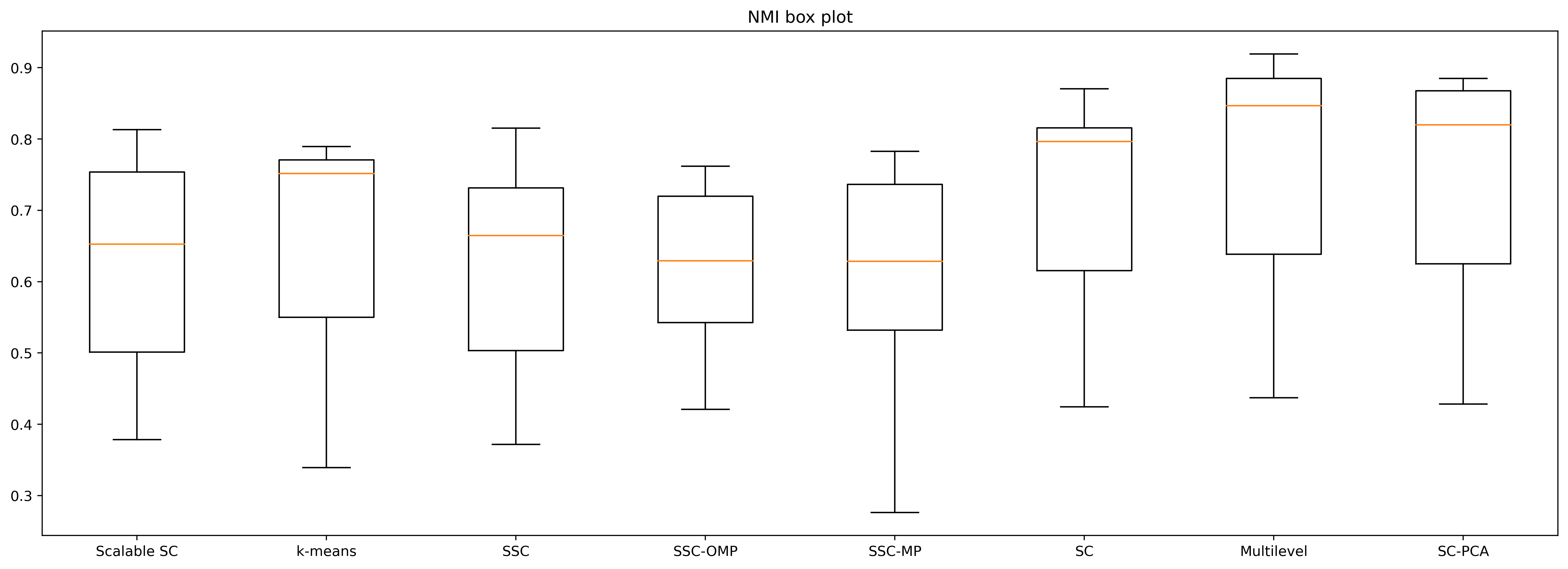
Figure 1: NMI Box Plot.

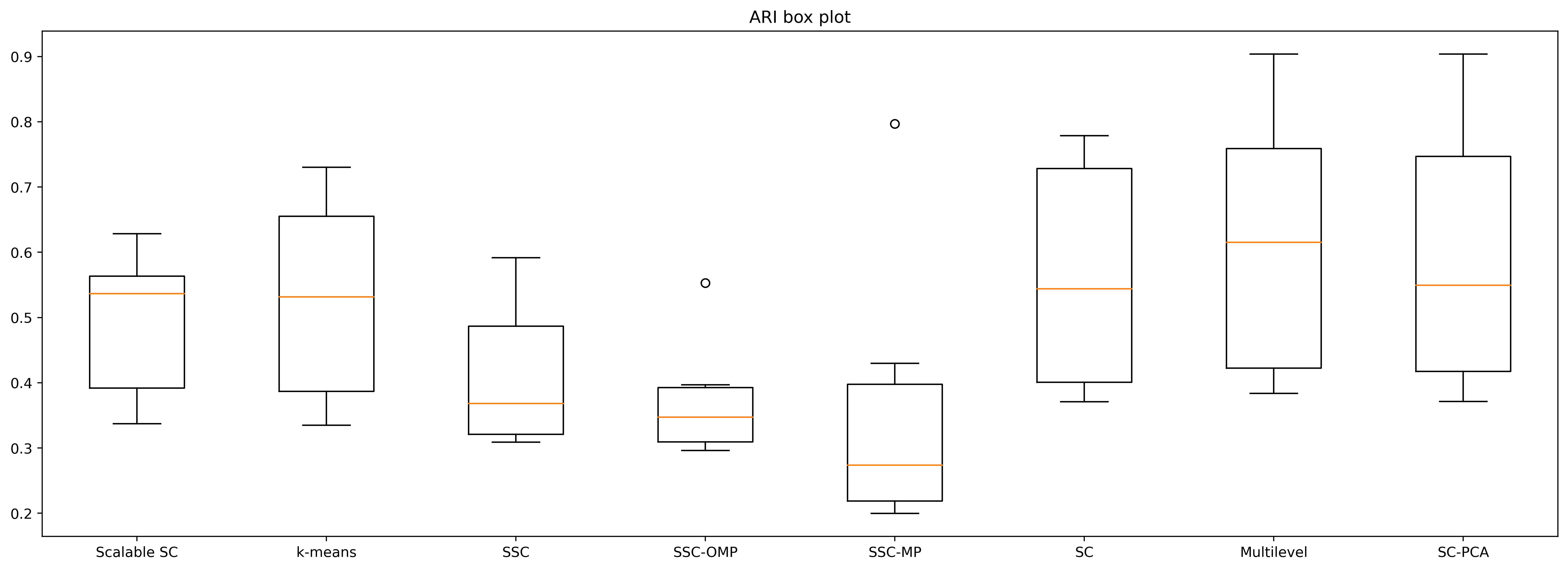
Figure 2: ARI Box Plot.

5 Conclusion

In this work, we have proposed two novel nonlinear spectral clustering models. The first model of proposed methods simultaneously uses global and local structure preservation for providing comprehensive structure information of the data to cluster nonlinear data by employing PCA, which makes the global properties to be considered in spectral clustering. Moreover, we introduce a multilevel model of our proposed technique for the nonlinear clustering that is solved by arithmetic mean points level by level to obtain a better clustering. Experimental results on six data sets have shown employing comprehensive information is important to improving clustering performance. In the future work, we intend to extend our proposed method into data manifolds with unknown structures by conformal mapping to provide a feature space with known structures.

References

- [1] Z. Bu, H.-J. Li, J. Cao, Z. Wang, G. Gao, Dynamic cluster formation game for attributed graph clustering, IEEE transactions on cybernetics 49 (1) (2017) 328–341.
- [2] F. Zhao, J. Fan, H. Liu, R. Lan, C. W. Chen, Noise robust multiobjective evolutionary clustering image segmentation motivated by the intuitionistic fuzzy information, IEEE Transactions on Fuzzy Systems 27 (2) (2018) 387–401.
- [3] C.-C. Li, Y. Dong, F. Herrera, A consensus model for large-scale linguistic group decision making with a feedback recommendation based on clustered personalized individual semantics and opposing consensus groups, IEEE Transactions on Fuzzy Systems 27 (2) (2018) 221–233.
- [4] I. S. Dhillon, Y. Guan, B. Kulis, Weighted graph cuts without eigenvectors a multilevel approach, IEEE transactions on pattern analysis and machine intelligence 29 (11) (2007) 1944–1957.
- [5] X. Zhu, C. Change Loy, S. Gong, Constructing robust affinity graphs for spectral clustering, in: Proceedings of the IEEE conference on computer vision and pattern recognition, 2014, pp. 1450–1457.
- [6] G. Chen, Scalable spectral clustering with cosine similarity, in: 2018 24th International Conference on Pattern Recognition (ICPR), IEEE, 2018, pp. 314–319.
- [7] J. Yan, M. Pollefeys, A general framework for motion segmentation: Independent, articulated, rigid, non-rigid, degenerate and non-degenerate, in: European conference on computer vision, Springer, 2006, pp. 94–106.
- [8] T. Zhang, A. Szlam, Y. Wang, G. Lerman, Hybrid linear modeling via local best-fit flats, International journal of computer vision 100 (3) (2012) 217–240.
- [9] L. Zelnik-Manor, M. Irani, Degeneracies, dependencies and their implications in multi-body and multi-sequence factorizations, in: 2003 IEEE Computer Society Conference on Computer Vision and Pattern Recognition, 2003. Proceedings., Vol. 2, IEEE, 2003, pp. II–287.
- [10] G. Chen, G. Lerman, Spectral curvature clustering (scc), International Journal of Computer Vision 81 (3) (2009) 317–330.
- [11] E. Elhamifar, R. Vidal, Sparse subspace clustering, in: 2009 IEEE Conference on Computer Vision and Pattern Recognition, 2009, pp. 2790–2797. doi:10.1109/CVPR.2009.5206547.
- [12] M. Soltanolkotabi, E. J. Candes, A geometric analysis of subspace clustering with outliers, The Annals of Statistics 40 (4) (2012) 2195–2238.
- [13] P. Favaro, R. Vidal, A. Ravichandran, A closed form solution to robust subspace estimation and clustering, in: CVPR 2011, IEEE, 2011, pp. 1801–1807.
- [14] C. You, D. Robinson, R. Vidal, Scalable sparse subspace clustering by orthogonal matching pursuit, in: Proceedings of the IEEE conference on computer vision and pattern recognition, 2016, pp. 3918–3927.
- [15] M. Tschannen, H. Bölcskei, Noisy subspace clustering via matching pursuits, IEEE Transactions on Information Theory 64 (6) (2018) 4081–4104.
- [16] M. Alshammari, J. Stavrakakis, M. Takatsuka, Refining a k-nearest neighbor graph for a computationally efficient spectral clustering, Pattern Recognition 114 (2021) 107869.
- [17] Z. Wang, S. Zhao, Z. Li, H. Chen, C. Li, Y. Shen, Ensemble selection with joint spectral clustering and structural sparsity, Pattern Recognition (2021) 108061.
- [18] K. Song, X. Yao, F. Nie, X. Li, M. Xu, Weighted bilateral k-means algorithm for fast co-clustering and fast spectral clustering, Pattern Recognition 109 (2021) 107560.
- [19] L. Zelnik-Manor, P. Perona, Self-tuning spectral clustering. advanced in neural information processing systems.
- [20] Q. Wang, C. Downey, L. Wan, P. A. Mansfield, I. L. Moreno, Speaker diarization with lstm, in: 2018 IEEE International Conference on Acoustics, Speech and Signal Processing (ICASSP), IEEE, 2018, pp. 5239–5243.
- [21] B. Long, Z. Zhang, X. Wu, P. S. Yu, Spectral clustering for multi-type relational data, in: Proceedings of the 23rd international conference on Machine learning, 2006, pp. 585–592.
- [22] F. Nie, G. Cai, X. Li, Multi-view clustering and semi-supervised classification with adaptive neighbours, in: Thirty-first AAAI conference on artificial intelligence, 2017.
- [23] H. Zeng, Y.-m. Cheung, Feature selection and kernel learning for local learning-based clustering, IEEE transactions on pattern analysis and machine intelligence 33 (8) (2010) 1532–1547.
- [24] G. Wen, Y. Zhu, L. Chen, M. Zhan, Y. Xie, Global and local structure preservation for nonlinear high-dimensional spectral clustering, The Computer Journal.
- [25] X. Niyogi, X. He, Locality preserving projections, in: Neural information processing systems, Vol. 16, 2004.
- [26] Z. Zhao, L. Wang, H. Liu, J. Ye, On similarity preserving feature selection, IEEE Transactions on Knowledge and Data Engineering 25 (3) (2011) 619–632.
- [27] M. Meilă, J. Shi, A random walks view of spectral segmentation, in: International Workshop on Artificial Intelligence and Statistics, PMLR, 2001, pp. 203–208.
- [28] A. Y. Ng, M. I. Jordan, Y. Weiss, On spectral clustering: Analysis and an algorithm, in: Advances in neural information processing systems, 2002, pp. 849–856.
- [29] J. Shi, J. Malik, Normalized cuts and image segmentation, IEEE Transactions on pattern analysis and machine intelligence 22 (8) (2000) 888–905.
- [30] R. O. Duda, P. E. Hart, D. G. Stork, Pattern Classification (2nd Edition), 2nd Edition, Wiley-Interscience, 2000.
- [31] B. Jiang, C. Ding, B. Luo, Robust data representation using locally linear embedding guided pca, Neurocomputing 275 (2018) 523–532.
- [32] O. Kayo, Locally linear embedding algorithm–extensions and applications.
- [33] H. G. Gene, F. Charles, et al., Matrix computations, Johns Hopkins Universtiy Press, 3rd edtion.
- [34] X. Liu, H.-M. Cheng, Z.-Y. Zhang, Evaluation of community detection methods, IEEE Transactions on Knowledge and Data Engineering 32 (9) (2019) 1736–1746.
- [35] R. Sinnott, H. Duan, Y. Sun, Chapter 15-a case study in big data analytics: exploring twitter sentiment analysis and the weather, Big Data (2016) 357–388.
- [36] J. A. Hartigan, M. A. Wong, Algorithm as 136: A k-means clustering algorithm, Journal of the royal statistical society. series c (applied statistics) 28 (1) (1979) 100–108.
- [37] Y. C. Pati, R. Rezaiifar, P. S. Krishnaprasad, Orthogonal matching pursuit: Recursive function approximation with applications to wavelet decomposition, in: Proceedings of 27th Asilomar conference on signals, systems and computers, IEEE, 1993, pp. 40–44.
-
[38]
J. H. Friedman, W. Stuetzle,
Projection pursuit regression,
Journal of the American Statistical Association 76 (376) (1981) 817–823.
URL http://www.jstor.org/stable/2287576 - [39] S. G. Mallat, Z. Zhang, Matching pursuits with time-frequency dictionaries, IEEE Transactions on signal processing 41 (12) (1993) 3397–3415.