Electroanatomic Mapping to determine Scar Regions in patients with Atrial Fibrillation

Abstract

Left atrial voltage maps are routinely acquired during electroanatomic mapping in patients undergoing catheter ablation for atrial fibrillation. For patients, who have prior catheter ablation when they are in sinus rhythm, the voltage map can be used to identify low voltage areas using a threshold of 0.2 - 0.45 mV. However, such a voltage threshold for maps acquired during atrial fibrillation has not been well established. A prerequisite for defining a voltage threshold is to maximize the topologically matched low voltage areas between the electroanatomic mapping acquired during atrial fibrillation and sinus rhythm. This paper demonstrates a new technique to improve the sensitivity and specificity of the matched low voltage areas. This is achieved by computing omni-directional bipolar voltages and applying Gaussian Process Regression based interpolation to derive the AF map. The proposed method is evaluated on a test cohort of 7 male patients, and a total of 46,589 data points were included in analysis. The low voltage areas in the posterior left atrium and pulmonary vein junction are determined using the standard method and the proposed method. Overall, the proposed method showed patient-specific sensitivity and specificity in matching low voltage areas of 75.70% and 65.55% for a geometric mean of 70.69%. On average, there was an improvement of 3.00% in the geometric mean, 7.88% improvement in sensitivity, 0.30% improvement in specificity compared to the standard method. The results show that the proposed method is an improvement in matching low voltage areas. This may help develop the voltage threshold to better identify low voltage areas in the left atrium for patients in atrial fibrillation.

I Introduction

The voltage map is one form of data provided by electroanatomic mapping (EAM) and is often used to demarcate low voltage areas (LVAs) and preserved voltage areas during catheter ablation therapy to treat atrial fibrillation (AF). low voltage areas correspond to areas of diseased atrium (fibrosis) or dense scars from prior ablations. Identifying LVA can help in planning ablation strategies especially in patients requiring repeat ablation procedures for arrhythmia recurrences, for example, AF and atypical atrial flutter.

The cutoff threshold voltage for a voltage map that determines LVAs has been established for maps obtained while the patient is in sinus rhythm (SR) [1][2]. However, this same threshold is not applicable to maps collected during AF.

For example, Fig. 1(a) depicts the SR map with a cutoff threshold of 0.45 mV. The regions below the threshold are clearly delineated from the healthy regions (magenta). However, in (b), applying the same threshold to the AF map for the same patient distorts the LVAs distribution. After adjusting to a lower threshold, as in (c), the LVAs on the AF map are restored to match the SR map.

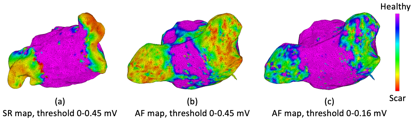
Figure 1: Example of need for a threshold to be used on voltage maps obtained during AF. Magenta area is healthy tissue, other colors are scar tissue. (a) The SR cutoff threshold of 0.45 mV is applied to the SR map. (b) Applying the same threshold to the AF map distorts LVAs in the AF map. (c) Adjusting the threshold to 0.16 mV restores the LVAs.

Several studies have shown that the local atrial signal acquired during AF is lower than in SR. Thus, identifying LVA during EAM in AF should require a lower cutoff voltage [3]. However, determining a consistent threshold that can be applied to all patients remains challenging. A prerequisite is determining the best match of LVAs that can be obtained between the SR map and the AF map and thereby finding the best threshold to be applied on a patient-by-patient basis.

Problem Statement: Given a set of measurements during SR and AF for a patient, maximize the topologically matched LVAs between the derived SR and AF map and determine the best patient-specific cutoff voltage threshold.

In this paper, we demonstrate a method of deriving the AF map which is robust to noise and error in the measurements and improves the patient-specific sensitivity and specificity of matched LVAs in comparison to the standard method through the following the contributions:

• Compute omni-directional bipolar voltages which are invariant to the orientation of the catheter, thus improving signal strength during AF.

• Apply Gaussian process regression (GPR) interpolation which improves the accuracy of LVA detection in regions of the atrium with lower measurement density.

II Background: Standard voltage map

Fig. 2 depicts the steps of deriving the current standard left atrial (LA) voltage map during catheter ablation of AF. Initially, as in (1), a 3D anatomical mesh is generated by manipulating a multi-electrode mapping catheter (Lasso or Pentaray) to different parts of the LA [4]. As the mesh is being created, recordings of 2.5 seconds of electrogram are collected at various locations around the endocardium. (2) shows the locations of all such sampled points on the LA mesh. The voltage value is interpolated to the remaining areas of the mesh to derive the final voltage map as shown in (3). The colors of the voltage map are based on a pre-specified cutoff threshold, where areas above the threshold are marked in magenta, and areas below the threshold are considered LVAs.

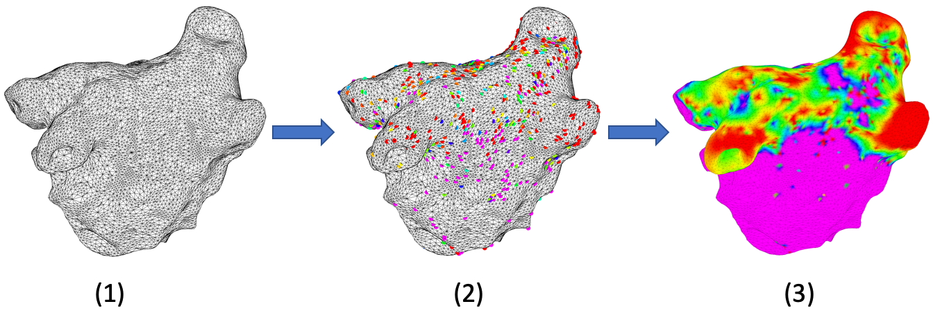
Figure 2: Standard method of deriving voltage map. (1) Anatomical mesh is computed from catheter locations. (2) Bipolar voltages are computed from measurements of electrogram at points along the mesh. (3) The bipolar voltages are interpolated to the remainder of the mesh to derive the voltage map.

Fig. 3 shows that within the 2.5 seconds, a 300 ms time window is defined relative to the QRS peak, and the peak-to-peak voltage is computed within the time window.

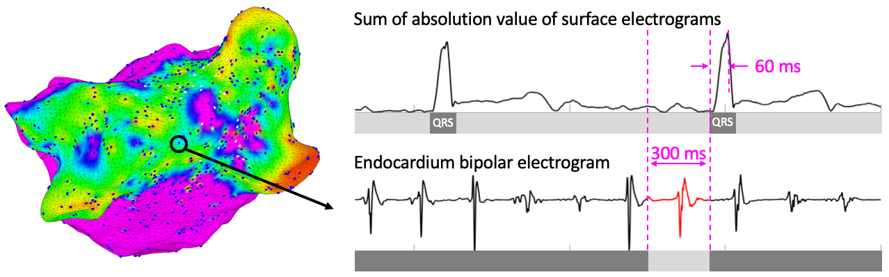
Figure 3: Bipolar voltages are computed as the peak-to-peak voltage in a pre-specified window within a 2.5 seconds recording of the endocardium electrogram.

III Robust Method for Voltage Map Derivation

Our proposed robust method deriving the voltage map differs from the standard method in terms of two components: a) omni-directional bipolar voltage and b) GPR-based interpolation.

a) Omni-directional bipolar voltage: Fig. 4 shows a limitation of bipolar recording, the dependency on electrode orientation. If the bipolar placement is parallel to the iso-electric potential line, the bipolar recording will be zero, which does not reflect the local electric activity [5]. To reduce such dependency, we derive the omni-directional bipolar voltage. For each sample point, we select the unipolar electrogram recorded in the vicinity of the sample and compute all possible bipolar electrogram from this set. We approximate the omni-directional bipolar voltage as the largest bipolar amplitude from this set. Fig. 4 (1) Blue depicts the histogram of the voltages for a patient. Red shows how the corresponding voltages are amplified. In the tail portion, the voltages of some LVA have increased above the threshold to be classified as healthy tissue. (2) and (3) exemplifies how the original red areas of voltage $\sim$0.06 mV are enhanced into yellow and green areas of voltage $\sim$0.17 mV.

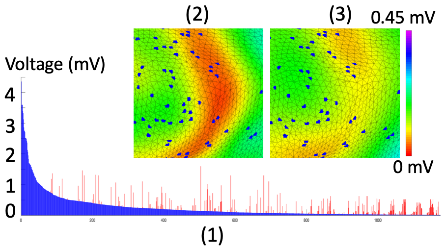
Figure 4: Benefits of using omni-directional bipolar voltages. (1) Bipolar voltages in AF (blue) are amplified (red), improving the signal. (2), (3) Regions of previously low voltage (red in (2)) are increased after computing omni-directional bipolar voltages (yellow in (3)).

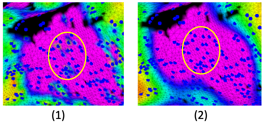
Figure 5: Standard interpolation vs. GPR-based interpolation. (1) Due to interpolation error, the circled region is determined as a LVA. (2) GPR-based interpolation accounts for measurements in the vicinity and reduces the LVA in the circled region.

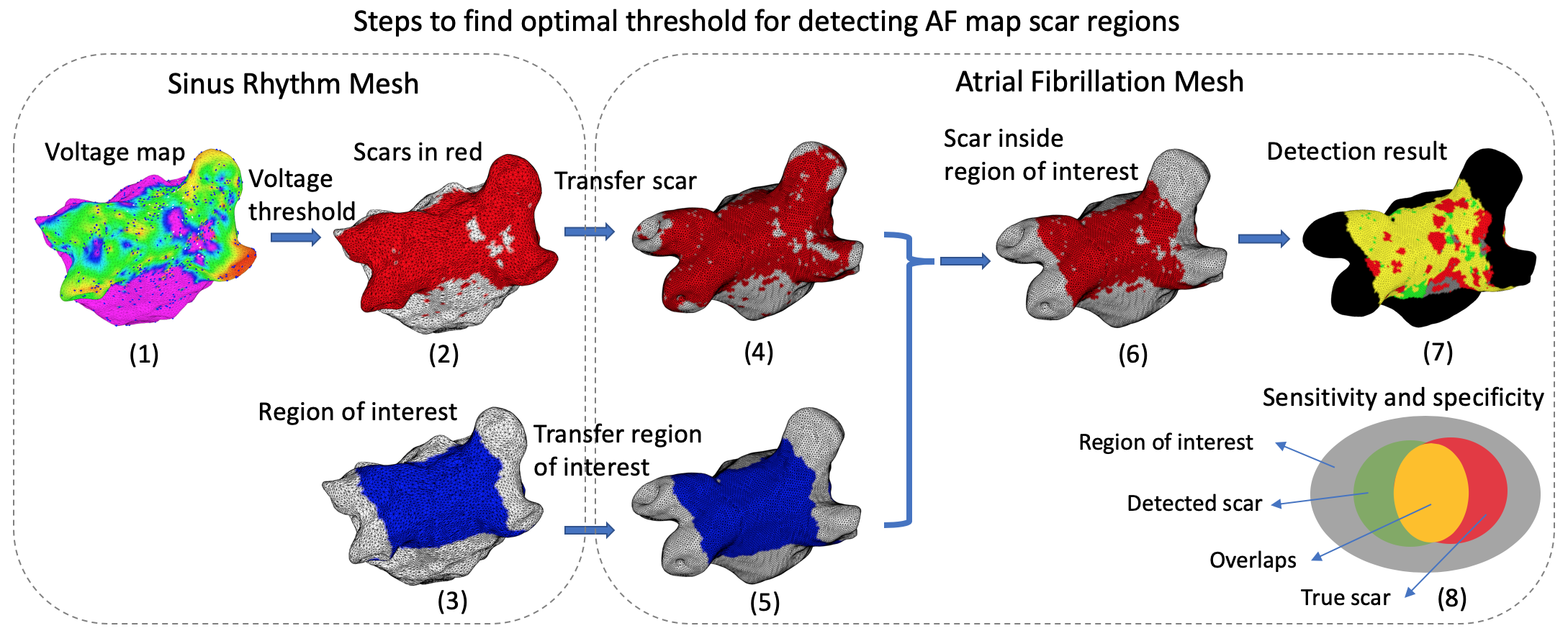
Figure 6: Experimental setup. For each patient: From the SR map (1), LVA are determined (2) as well as the region of interest (3). Both (2) and (3) are topologically transferred to the AF map (4) and (5). (4) (5) are intersected to obtain the true LVAs on the AF map (6). The optimal patient-specific threshold is determined by maximizing the product of sensitivity and specificity accordin to (8).

b) Gaussian process regression based interpolation: If we model the endocardium as a surface and define the entire set of samples as, $\mathcal{D}=\{\mathbf{x}_{n},y_{n}\}^{N}_{n=1}$, where inputs $\mathbf{X}=\{\mathbf{x}_{n}\}^{N}_{n=1}$ correspond to the locations on the mesh and $\mathbf{y}=\{y_{n}\}^{N}_{n=1}$ are the voltage value at that location. Interpolating from these measured samples to the remainder of the mesh can be thought of as determining the estimates of the voltages at locations $\mathbf{X^{*}}$. The two major sources of interpolation error are the low measurement density and measurement noise. Both of these can be accounted for by modeling them using a Gaussian process $GP(m(\mathbf{x},k(\mathbf{x},\mathbf{x}^{\prime})))$ [6], which is characterized by the mean $m(\mathbf{x})$ and the covariance $k(\mathbf{x},\mathbf{x}^{\prime})$ kernel functions. We assume the common zero mean function and use the squared exponential function $k(\mathbf{x},\mathbf{x}^{\prime})=\exp(-||\mathbf{x}-\mathbf{x}^{\prime}||/(2\cdot l^{2}))$. Fig. 5(1) shows how the standard interpolation can result in regions that are classified as LVAs, due to interpolation error. (2) shows GPR-based interpolation can improve the boundaries of LVAs by considering the surrounding measurements.

For determining the optimum threshold, a search in the range of 0-0.45 mV is performed to maximize the product of sensitivity and specificity. Here, sensitivity $=\frac{\text{TP}}{TP+FN}$ and specificity $=\frac{\text{TN}}{TN+FP}$, where a true positive (TP) indicates that the corresponding face on the anatomical mesh is detected as a LVA and the true label is a LVA.

The proposed method of voltage map derivation was evaluated on a test cohort of 7 patients that underwent repeat catheter ablation for AF at the Hospital of the University of Pennsylvania. Patient demographics are: age $66\pm 0.7$ years, height $5^{\prime}10"\pm 4"$, weight $238.9\pm 50$ lb and ejection fraction $49.4\%$. Details are in Table I. For each patient, voltage maps were sequentially obtained using Carto3 (Biosense Webster) during SR and AF or vice-versa. Fill threshold was 5 mm, and filters were set at 2 to 240 Hz for unipolar electrograms, 16-500 Hz for bipolar EGMs, and 0.5-200 Hz for surface electrogram recordings. We assumed that the LVA observed based on the SR voltage map is the ground truth.

Patient	1	2	3	4	5	6	7
Age	66	58	70	70	69	58	76
Height (inch)	71	75	72	62	70	72	68
Weight (pound)	290	260	266	243	267	200	146
Ejection Function (%)	65	50	25	50	55	60	40

TABLE I: Patient population

IV Experimental setup

The overall evaluation process is depicted in Fig. 6. From the original data (1), we apply the standard 0.45 mV cutoff threshold on the SR map to identify regions of LVA (2). We select a region of interest (ROI) on the SR map (3), which consists of the posterior LA and pulmonary vein (PV) junctions. Both the LVA and the ROI is transferred to the AF mesh and intersected to form the final LVA on the AF map (4),(5),(6). Then result (7) is determined as shown in (8) in terms of sensitivity and specificity.

V Results and discussion

A total of 46,589 data points were included in analysis, that was on average 6,656 data points for each of the 7 patients. Table II summarizes the results of evaluation for each patient. On average, our proposed method showed a sensitivity and specificity of 75.70% and 66.55%, respectively. This was a 3.00% improvement in the geometric mean compared to the standard method. Moreover, our proposed method exhibited a 7.88% improvement in sensitivity and a 0.30% improvement in specificity. ROC curves were obtained for each of the methods and the area under the curve was computed as shown in Fig. 7. Our proposed method showed an average of 3.91% improvement in terms of the area under the curve (AUC).

Patient	Baseline					Omni.+GP					Percentage of Improvement
	Sens.	Spec.	GM	AUC	Voltage Threshold	Sens.	Spec.	GM.	AUC	Voltage Threshold	$\Delta$Sens.	$\Delta$Spec.	$\Delta$GM	$\Delta$AUC
1	76.18	63.56	69.58	0.77	0.26	84.92	70.74	77.51	0.85	0.23	11.47	11.30	11.40	10.39
2	54.87	57.64	56.24	0.57	0.09	72.72	47.49	58.77	0.61	0.11	32.53	-17.61	4.50	7.02
3	77.38	71.48	74.37	0.80	0.16	91.22	69.59	79.67	0.86	0.15	17.89	-2.64	7.13	7.50
4	79.52	78.08	78.80	0.85	0.26	85.42	77.07	81.14	0.89	0.30	7.42	-1.29	2.97	4.71
5	58.08	66.88	62.32	0.67	0.36	69.24	56.71	62.66	0.66	0.38	19.21	-15.21	0.55	-1.49
6	80.61	74.64	77.57	0.83	0.32	72.87	83.41	77.96	0.85	0.21	-9.60	11.75	0.50	2.41
7	70.24	52.57	60.77	0.63	0.10	53.54	60.87	57.09	0.61	0.17	-23.78	15.79	-6.06	-3.17
Average	70.98	66.41	68.52	0.73	0.22	75.70	66.55	70.69	0.76	0.22	7.88	0.30	3.00	3.91
Std	10.49	9.19	8.87	0.11	0.11	12.72	12.34	10.65	0.13	0.09	18.96	13.32	5.54	4.95

TABLE II: Results for patient-specific performance for all patients

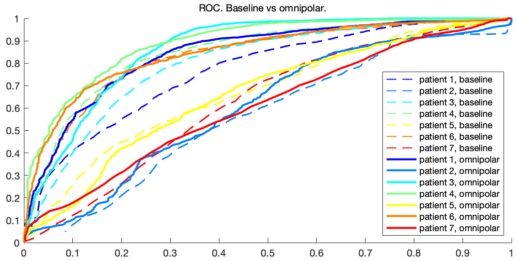
Figure 7: ROC curve comparing, baseline method vs proposed method using omni-directional bipolar voltages and GPR-based interpolation. The proposed method shows improved or similar performance across various thresholds.

Fig. 8 depicts patient 1 with the improved detection of LVAs after applying the optimal threshold. First, the improvement is due to the enhanced signal in the omni-directional bipolar voltages. On the boundaries of the ROI LVAs are correctly categorized as healthy regions using the proposed method. Second, in the areas of high electrode density, GPR-based interpolation discounts the amplitude when voltage spikes due to noise occur. Finally, in regions of lower measurement density, the standard method underestimates the interpolated voltage when spurious low-voltage measurement exist. In this case the combination of omni-directional bipolar voltages enhances the signal, and GPR-based interpolation filters such noise, preventing classification as LVAs.

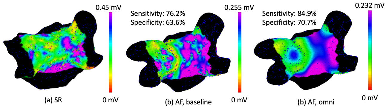
Figure 8: Example of improved result: Patient 1, baseline vs proposed method.

In patient 7, our proposed method did not improve performance. Upon further inspection, we discovered that 90% of the ROI was LVA as shown in Fig. 9. This patient had undergone prior extensive surgical ablation and so had extensive areas of dense scar in the ROI, making discrimination difficult. Optimizing the threshold with a different criterion which accounts for this bias may result in a better outcome.

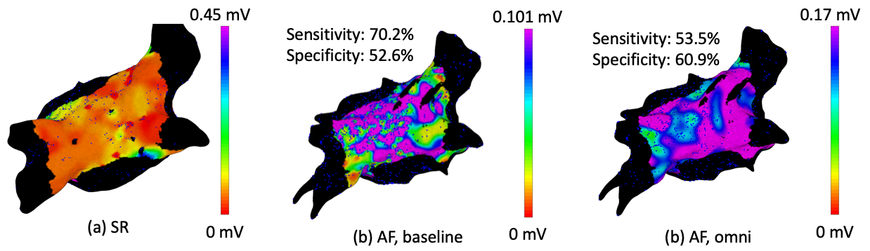
Figure 9: Patient 7. Baseline vs proposed method. Poor performance can be attributed to the dominance of LVAs in the ROI, thus penalizing specificity.

Limitations: The results of our study are limited in scope, mostly in part by the small cohort size. Bias due to the particular demographics of the cohort may have affected the results and different results may be obtained with a larger cohort. Selection of different hyperparameters for the method, such as a different kernel for GPR-based regression may affect the performance. Finally, establishing a standard protocol for obtaining data may lead to improvement.

VI Conclusion

In this work, we have presented a method for deriving the voltage map during AF and comparing it to voltage maps acquired during SR. Our method computes omni-directional bipolar voltages from the measurements and utilizes GPR-based interpolation to derive the voltage map. Evaluation on the test cohort showed that, in general, the method improved the patient-specific sensitivity and specificity in determining LVAs of the AF map compared to the standard method, though some exceptions exist. This improvement in matched areas between the maps is significant and has important practical implications as clinicians interpret voltage maps according to the areas and not by the individual point measurements. More accurate information about LVA distribution is helpful to clinicians in planning ablation strategies for patients who require repeat catheter ablation for arrhythmia recurrences. Immediate future work is to apply the method over a larger cohort. In a practical clinical setting, patient-to-patient variability may need to be accounted for in the criterion. Overall, the results provide evidence that the proposed method improves the detection of LVAs in AF maps. Because of the robustness to measurement noise and interpolation error, the proposed method could lead to a more consistent criterion.

References

- [1] S. Kapa et al., “Contact electroanatomic mapping derived voltage criteria for characterizing left atrial scar in patients undergoing ablation for atrial fibrillation,” Journal of Cardiovascular Electrophysiology, vol. 25, no. 10, pp. 1044–1052, 2014.
- [2] F. Squara et al., “Voltage mapping for delineating inexcitable dense scar in patients undergoing atrial fibrillation ablation: A new end point for enhancing pulmonary vein isolation,” Heart Rhythm, vol. 11, no. 11, pp. 1904 – 1911, 2014.
- [3] Rodríguez-Mañero et al., “Validating left atrial low voltage areas during atrial fibrillation and atrial flutter using multielectrode automated electroanatomic mapping,” JACC: Clinical Electrophysiology, vol. 4, no. 12, pp. 1541 – 1552, 2018.
- [4] J. J. Liang et al., “Comparison of left atrial bipolar voltage and scar using multielectrode fast automated mapping versus point-by-point contact electroanatomic mapping in patients with atrial fibrillation undergoing repeat ablation,” Journal of Cardiovascular Electrophysiology, vol. 28, no. 3, pp. 280–288, 2017.
- [5] K. Magtibay et al., “Resolving bipolar electrogram voltages during atrial fibrillation using omnipolar mapping,” Circulation., vol. 10, no. 9, 2017-09.
- [6] C. E. Rasmussen and C. K. I. Williams, Gaussian processes for machine learning. Adaptive computation and machine learning, Cambridge, Mass: MIT Press, 2006.