kafe2 - a Modern Tool for Model Fitting in Physics Lab Courses

Abstract

Fitting models to measured data is one of the standard tasks in the natural sciences, typically addressed early on in physics education in the context of laboratory courses, in which statistical methods play a central role in analysing and interpreting experimental results. The increased emphasis placed on such methods in modern school curricula, together with the availability of powerful free and open-source software tools geared towards scientific data analysis, form an excellent premise for the development of new teaching concepts for these methods at the university level. In this article, we present kafe2, a new tool developed at the Faculty of Physics at the Karlsruhe Institute of Technology, which has been used in physics laboratory courses for several years. Written in the Python programming language and making extensive use of established numerical and optimization libraries, kafe2 provides simple but powerful interfaces for numerically fitting model functions to data. The tools provided allow for fine-grained control over many aspects of the fitting procedure, including the specification of the input data and of arbitrarily complex model functions, the construction of complex uncertainty models, and the visualization of the resulting confidence intervals of the model parameters.

1 Model fitting in lab courses: pitfalls and limitations

A primary goal of data analysis in physics is to check whether an assumed model adequately describes the experimental data within the scope of their uncertainties. A regression procedure is used to infer the causal relationships between independent and dependent variables, the abscissa values $x_{i}$ and the ordinate values $y_{i}$. The dependency is typically represented by a functional relation $y_{i}=f(x_{i};\{p_{k}\})$ with a set of model parameters $\{p_{k}\}$. Both the $y_{i}$ and the $x_{i}$ are the results of measurements and hence are affected by unavoidable measurement uncertainties that must be taken into account when determining confidence intervals for the model parameters. It has become a common standard in the natural sciences to determine confidence intervals for the parameter values based on a maximum-likelihood estimation (MLE). In practice, one typically uses the negative logarithm of the likelihood function (NLL), which is minimised by means of numerical methods.

In the basic laboratory courses, parameter estimation is traditionally based on the method of least squares (LSQ), which in many cases is equivalent to the NLL method. For example, fitting a straight line to data affected by static Gaussian uncertainties on the ordinate values $y_{i}$ is an analytically solvable problem and the necessary calculations can be carried out by means of a pocket calculator or a simple spreadsheet application. For simplicity, non-linear problems are often converted to linear ones by transforming the $y$ values. However, the Gaussian nature of the uncertainties is lost in this process, which is why the transformed problem only gives accurate results if the uncertainties are sufficiently small. Simple error propagation is often used to transform the fitted parameters like the slope or $y$ intercept to the model parameters of interest. As a result, the parameter uncertainties obtained in this way are no longer Gaussian, and it is non-trivial to determine sensible confidence intervals. When the independent variables are also affected by measurement uncertainties, or when relative uncertainties with respect to the true values are present, this traditional approach reaches its limits.

Such simple analytical methods are very limited in their general applicability to real-world problems. For instance, the presence of uncertainties on the abscissa values in addition to those on the ordinate values, as they would be encountered when measuring a simple current-voltage characteristic of an electronic component, already results in a problem that can generally no longer be solved analytically. Unfortunately, most of the widely used numerical tools for parameter estimation provide only limited support for such non-linear problems, even though they occur frequently in practice.

Prior to drawing any conclusions on model parameters, the most important task in physics is to check the validity of a model hypothesis assumed to describe a set of measurement data. The full task therefore consists of the following steps:

1. carefully quantifying the uncertainties of all input measurements;

2. defining a model hypothesis for the measured data;

3. testing whether the measurements are compatible with the model hypothesis;

4. if so, determining the model parameters, e.g. the slope and intercept of a straight line.

It is precisely the hypothesis testing in step 3 that drives progress in scientific understanding by providing the relation between measurements and theoretical models. A simple example for such a hypothesis test is the $\chi^{2}$ test, which results directly from the frequently used method of least squares. A test for the validity of the model assumption should definitely be performed before drawing any conclusions from the values and uncertainties of the fitted model parameters. Unfortunately, many of the common tools come with a default setting that assumes the correctness of the given parameterization and scales the parameter uncertainties so that the model perfectly describes the data within the parameter uncertainties so determined. This behaviour can usually be switched off by choosing appropriate options, but in practice this is often neglected.

The parameters of a complex model can be highly correlated. In this case it is no longer sufficient to consider the distribution of just a single parameter. Instead the shared distribution of multiple parameters needs to be considered, for example when conducting hypothesis testing. Correlations between model parameters can also be problematic for numerical optimisation. For this reason strategies for choosing appropriate parameterizations to reduce these correlations also need to be addressed. It is then indispensable that the correlations are also shown when presenting the fit results. Ideally the correlation between two model parameters can be expressed with a simple correlation coefficient. However, if non-linear models are fitted, this is often not sufficient for the evaluation of the result; in this case the corresponding confidence regions should be determined and presented as contour graphs for pairs of parameters.

The distinction between ”statistical” and ”systematic” uncertainties leads to many misunderstandings among students. For example, the systematic error of a measuring instrument becomes a statistical one if several measuring instruments of the same type are used. A much more suitable approach is to differentiate whether uncertainties affect all measured values or groups of measured values equally or whether they are independent. This approach, however, requires dealing with the covariance matrix of measurement uncertainties and constructing it from the individual uncertainties on a problem-by-problem basis. Unfortunately, there are very few simple tools that allow a full covariance matrix to be considered in the fitting process. None of the tools commonly used in physics lab courses allow students to take into account correlated uncertainties of both the abscissa and ordinate values.

While there are tools with which the requirements listed here could be partially implemented, these do not provide the simplicity needed for undergraduate physics education. To address the issues described above it became necessary to write a tool of our own, kafe2, an open-source Python package designed to provide a flexible Python interface for the estimation of model parameters from measured data.

2 The Open-Source Python Package kafe2

After designing a prototype package, kafe, development continued with kafe2 [1]. Said tools make use of contemporary methods for visualization and evaluation of measurement data and are based on freely available, open-source software that is also used in scientific contexts and thus relevant for later professional practice.

2.1 Implementation

Due to its widespread use in scientific communities as well as in the burgeoning professional field of data science, Python [2] was chosen as the programming language for kafe2. As a high-level language with particular emphasis on clear and intuitive syntax, and convenient features such as dynamic typing and garbage collection, Python provides a beginner-friendly programming environment, requiring comparatively little knowledge to use effectively. This is particularly advantageous in a field such as physics, which requires a very broad foundation of knowledge prior to specialization and thus allows only a limited percentage of the curriculum to be assigned to programming.

However, an inevitable downside of Python is that it is comparatively slow compared to low-level languages such as C/C++. Fortunately, the Python ecosystem features many libraries for numerical computation, most notably the NumPy [3] library, which makes use of fast underlying C implementations for running such computations efficiently. Optimal use of these libraries does require some detailed knowledge, but in the case of kafe2 this generally only applies to development rather than use.

The numerical optimization algorithms necessary for finding the global minimum of the negative log-likelihood function are provided either by the library SciPy [5] (”scientific Python”) or by the Python package iminuit [6], which is based on the MINUIT package developed at CERN, the European Organization for Nuclear Research.

The graphics library matplotlib [4] is used as the graphical backend for publication quality visualizations of input data and results. kafe2 itself is implemented in pure Python and can therefore run on all common platforms with a Python environment, including ARM-based platforms such as the Raspberry Pi.

2.2 Special Features of kafe2

The kafe2 package provides numerous unique features that are listed in the following.

To represent complex uncertainty models with absolute and/or relative, independent and/or correlated uncertainties on abscissa and/or ordinate values, kafe2 uses two covariance matrices collecting the uncertainty components on the abscissa and ordinate directions. As described below, these are combined into a single overall covariance matrix used in the numerical regression. Users can specify multiple uncertainties of the same kind which are then automatically combined into the corresponding covariance matrices. If relative uncertainties are specified, they most often refer to the true values of the input data, which are only (approximately) known after the regression. kafe2 is able to handle such cases by dynamically calculating the uncertainties as relative to the model; optionally and for compatibility with other tools it is possible to use relative uncertainties with respect to the measured data. Correlations between uncertainty components or between individual uncertainties can be specified as a correlation coefficient or as a complete covariance matrix.

In addition to pre-defined, rather simple model functions, arbitrarily complex user-defined functions can be easily implemented using native Python syntax. It is also possible to simultaneously fit several model functions with shared parameters to data; this feature is very useful if auxiliary or external measurements of model parameters need to be considered. Fixing the values of one or more model parameters or constraining them within given external uncertainties is also supported.

The numerical fitting procedure in kafe2 relies on the NLL method, but falls back to the simple LSQ method if equivalent to NLL in order to avoid computationally expensive operations. Distributions can be fitted to binned data (histograms) using a Poisson likelihood; optionally and for compatibility with other packages the LSQ method can alternatively be chosen. kafe2 also supports fits with user-defined maximum-likelihood functions.

Parameter uncertainties are determined in the traditional way relying on the the Cramér-Rao-Fréchet bound, i.e. from the second derivatives of the LSQ or NLL function at the minimum. To deal with non-linear cases and correlated parameters, a likelihood-based method known as ”profile likelihood” is also optionally offered for determining parameter confidence intervals. In multi-parameter problems, this is also useful to account for the influence of nuisance parameters when determining individual parameter uncertainties.

Fit results are provided in graphical form, but output in text form is also possible. Access functions exist to extract results for further processing with Python code. If meaningful, kafe2 provides metrics to judge the goodness of a fit result. The output also includes the parameter correlations, as is standard for most other fitting tools. The graphical output shows the data and the best-fit model function with an optional representation of the model uncertainty as a shaded band. An optional graphical representation of the profile likelihood for each parameter and of confidence regions of pairs of parameters as contours are also provided.

More details on the mathematical procedures and a concrete application example are given below.

2.3 Mathematical procedures

The estimation of model parameters and their uncertainties in kafe2 is based on the method of maximum-likelihood estimation. Given a set of $N$ measurements $y_{i}$ with corresponding abscissa values $x_{i}$, as well as a model function $f({x_{i}},\{p_{k}\})$ depending on a set of parameters $\{p_{k}\}$, the most commonly assumed data distribution is the $N$-dimensional Gaussian distribution $\cal N$ with the uncertainties on the ordinate values being described by the covariance matrix $\bf V$:

$$\mathcal{N}\left(\{y_{i}\},f(\{x_{i}\},\{p_{k}\}),{\bf V}\right)\,=\,\displaystyle\frac{1}{\sqrt{(2\pi)^{N}\det{\bf V}}}\exp\left(-\frac{1}{2}\sum_{i,j=1}^{N}\left(y_{i}-f(x_{i},\{p_{k}\})\right)\left({\bf V}^{-1}\right)_{ij}\left(y_{j}-f(x_{j},\{p_{k}\})\right)\right)\,.$$

The cost function ${\cal{C}}$ to be minimized is defined as twice the negative logarithm of the likelihood ${\cal{L}}$ of $\cal N$, ${\cal{C}}=-2\ln{\cal{L}}$. Terms that are independent of the parameters are typically neglected in the definition of the likelihood since they are irrelevant for the location and shape of the global cost function minimum.

The total uncertainties of the measurement data are described by the covariance matrix ${\bf V}$. The uncertainties of the measurement points in the abscissa direction are described by a covariance matrix with elements ${\bf V}^{x}_{ij}$. Because the Gaussian likelihood is only defined for ordinate uncertainties kafe2 handles abscissa uncertainties by transforming them into ordinate uncertainties. This is achieved by multiplying them with the first derivatives of the model function. The resulting uncertainties are then simply added to the covariance matrix elements ${\bf V}^{y}_{ij}$ of the ordinate uncertainties. The elements of the total covariance matrix used in the fit are thus

$${\bf V}_{ij}={\bf V}^{y}_{ij}+{\bf V}^{x}_{ij}\cdot f^{\prime}(x_{i})\cdot f^{\prime}(x_{j})\,.$$

This approach assumes that, near the global cost function minimum, the fitted model function can be sufficiently well approximated by a straight line in the vicinity of the support points $x_{i}$, i.e. that second-order derivatives are negligible on the scale of the abscissa uncertainties $\Delta x_{i}$.

For uncertainties that are independent of the parameter values, ${\cal{C}}$ is equivalent to the method of least squares, which is classically used as the cost function in most fitting algorithms,

$${\cal{C}}(\{y_{i}\},{\bf V}^{y},f(\{x_{i}\},\{p_{k}\}))\,=\,\displaystyle\sum_{i,j}\left(y_{i}-f(x_{i},\{p_{k}\})\right)\left(\big{(}{{\bf V}^{y}}\big{)}^{-1}\right)_{ij}\left(y_{j}-f(x_{j},\{p_{k}\})\right)\,.$$

The expected value of ${\cal{C}}$ for the best parameter values estimated from a hypothetical set of data follows a $\chi^{2}$-distribution with a number of degrees of freedom (NDF) corresponding to the difference between the number of data points and the number of free model parameters. The ratio $\mathcal{C}/\mathrm{NDF}$, often called the ”reduced $\chi^{2}$”, has an expectation value of unity for a model that accurately describes the data within their uncertainties. The ”$\chi^{2}$ probability” $p=1-q$ is determined from the quantile $q$ of the $\chi^{2}$ distribution for the observed minimum and can be used to quantify the goodness-of-fit. If, however, the uncertainties do depend on the parameters, as is for instance the case for relative ordinate uncertainties or uncertainties on the abscissa values, then the method of least squares is no longer equivalent to the method of maximum likelihood. This is because the normalization term of the multivariate Gaussian, which is a function of $\det\left(\bf V(\{p_{k}\})\right)$, must also be taken into account. While a parameter-dependent covariance matrix needs to be recomputed on every parameter change, thus adding to the computational cost of the minimization, it remains feasible on modern hardware, particularly if the inversion of the covariance matrix $\bf V$ is replaced by a Cholesky decomposition ${\bf L}{\bf L}^{T}={\bf V}$. In addition, the Cholesky decomposition also enables the quick computation of the covariance matrix determinant by exploiting that $\bf L$ is a triangular matrix: $\det\left({\bf V}\right)=\det\left({\bf L}\right)\cdot\det\left({\bf L}^{T}\right)=2\det\left({\bf L}\right)$.

Following common standards based on the Cramér-Rao-Fréchet bound, an estimate of the covariance matrix of the parameter uncertainties is determined from the inverse Hessian matrix, containing the second-order derivatives of ${\cal{C}}(\{y_{i}\},V,f(\{x_{i}\};\{p_{k}\}))$ with respect to the parameters $p_{k}$. In general, however, this approach is not sufficient for reliably determining the confidence intervals of the fitted parameters. For this reason, kafe2 also implements the profile likelihood method. The so-called profile as a function of a subset of the parameters is determined by keeping the values of these parameters fixed and minimizing ${\cal{C}}$ with respect to all other parameters. The boundaries of a confidence interval are determined by finding the locus of points for which the profile likelihood increases by a value $\Delta\mathcal{C}$ with respect to the global minimum. In the case of two parameters, this amounts to finding the intersection of the two-dimensional profile likelihood function with a horizontal plane above the global cost function minimum.

The value of $\Delta{\cal{C}}$ determines the confidence level of the confidence interval/region. For example, for a one-dimensional confidence interval $\Delta{\cal{C}}=1$ corresponds to the $1\,\sigma$ interval of a Gaussian distribution with a confidence level of 68.3%, where $\sigma$ is the standard deviation of the one-dimensional Gaussian distribution. In the two-dimensional case (as in the profile likelihood of two parameters) the intersection of a two-dimensional profile likelihood with a horizontal plane is a one-dimensional curve. This curve corresponds to a confidence contour, which is an ellipse in case of Gaussian uncertainties. If the contour deviates strongly from the elliptical form, is no longer possible to correctly specify a confidence region of the two parameters by providing a simple correlation coefficient. In this case, the contour plots of the affected pairs of parameters as well as the one-dimensional confidence intervals should be documented.

The profile likelihood method is important because non-linear problems are very common in practice. Even a simple linear regression with additional uncertainties on the abscissa values leads to a non-linear problem for which no general analytical solution exists. Relative uncertainties on the ordinate values introduce similar issues. They should be specified relative to the model (as a stand-in for the unknown ”true values”) to avoid the bias which otherwise would give too much weight to data points with downward fluctuations of the measured values and hence the assigned uncertainties. When the model function itself is nonlinear in the parameters or when abscissa uncertainties or relative ordinate uncertainties are used, the shape of the covariance contours should always be inspected. Using appropriate tools, the associated calculations usually only take on the order of seconds on consumer hardware. An example with kafe2 is shown below.

In addition to the Gaussian-based cost functions discussed until now, kafe2 also offers other cost functions, for example a cost function based on the Poisson distribution for fitting models to frequency distributions (histograms). The specification of user-defined cost functions is also possible; in order to benefit from the statistical interpretation of the fit results provided by kafe2, such cost functions must be based on valid likelihood functions.

Often it is desirable to show the uncertainty of the fitted model function. An approximate confidence region $\Delta f(x;p)$ can be derived from the covariance matrix, ${\bf V}^{p}$, of the model parameters and the gradient, $\nabla_{p}f(\{x_{i}\};\{p_{k}\})$, of the model function with respect to the parameters by (linear) propagation of the uncertainties:

$$\Delta f(x_{i},\{p_{k}\})=\Big{(}\nabla_{p}f(x_{i};\{p_{k}\})\Big{)}^{T}{\bf V}^{p}\ \nabla_{p}f(x_{i};\{p_{k}\})\,.$$

3 User interface and applications

To mitigate the inherent trade-off between usability and complex functionality kafe2 offers the user several interfaces for fitting:

• For those without programming knowledge, or for the convenience of advanced users, a command line interface “kafe2go” is provided. Users only need to supply a configuration file in the format of the widely used data serialization language YAML [8], which specifies the data, the model function and fitting options.

• More flexibility is offered to slightly advanced users with basic programming knowledge; they can call the Python interface of built-in kafe2 pipelines as part of a larger Python script.

• Advanced users have the possibility to construct custom pipelines by directly instantiating the kafe2 objects that represent input data, model functions, fits or graphical output.

As an example, the stand-alone application kafe2go can be used via the following command line call:

kafe2go <name>.yaml.

Figure 1 illustrates the result of fitting a straight line to data points with uncertainties in both the ordinate and abscissa directions. The input file contains only the following lines:

 # input data straight line fitting
 x_data: [1.0, 2.0, 3.0, 4.0]
 x_errors: 5%
 y_data: [2.3, 4.2, 7.5, 9.4]
 y_errors: 0.4
 

Note: if no model function is specified, kafe2go defaults to a first-degree polynomial as the model.

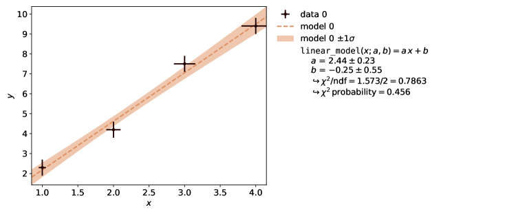
Figure 1: Graphical output of kafe2. The shaded region around the fitted straight line shows the 68% confidence interval of the model function.

When using kafe2 as a Python library, a Jupyter [9] environment is very convenient. One advantage is that this allows users to combine text, program code and outputs in a so-called ”Jupyter notebook”. A second advantage is that it also enables teaching staff to provide the entire Python environment for running kafe2 as a service to students; the students themselves only need to connect to a Jupyter server via web browser without the need to spend time setting up a Python environment themselves.

To use the built-in kafe2 pipelines for model fitting, users simply need to call the corresponding functions. The creation of custom pipelines, however, requires a more advanced understanding of object-oriented programming. First, a data container object is instantiated from numerical input data and their uncertainties. Then a fit object is created from a data container object and a model function. After possibly constraining or limiting parameters via dedicated method calls, the method do_fit() is called to perform the numerical optimization of the cost function. The fit results are then accessed via the corresponding attributes of the fit object or printed to console by calling the report() method. In order to create a graphical representation of the fit results a plot object can be instantiated from the fit object. A complete code example, which corresponds exactly to the one just discussed and leads to the same graphical output as in Figure  1, looks as follows:

    # Python code for fitting a straight line
    from kafe2 import XYContainer, Fit, Plot
    xy_data = XYContainer(
        x_data=[1.0, 2.0, 3.0, 4.0],
        y_data=[2.3, 4.2, 7.5, 9.4]
    )
    xy_data.add_error(
        axis=’x’,
        err_val=0.05,
        relative=True
    )
    xy_data.add_error(
        axis=’y’,
        err_val=0.4
    )
    line_fit = Fit(xy_data)
    line_fit.do_fit()
    line_fit.report()
    plot = Plot(fit_objects=line_fit)
    plot.plot()
    plot.show()

Since fits of models to two-dimensional data points is a very common use case a built-in function implementing the pipeline is also available:

    import kafe2
    kafe2.xy_fit(
        x_data=[1.0, 2.0, 3.0, 4.0],
        y_data=[2.3, 4.2, 7.5, 9.4],
        x_error_rel=0.05,
        y_error=0.4
    )
    kafe2.plot()

Because relative abscissa uncertainties are specified (via x_error_rel), the built-in pipeline automatically switches to calculating parameter uncertainties with the profile likelihood. A plot of the confidence intervals/regions is also created automatically.

Users are provided with several resources to familiarize themselves with the use of kafe2. In addition to the traditional documentation explaining the use by showing examples there is also a tutorial in the form of a Jupyter notebook that takes a more interactive approach. Among others, the following topics are covered:

1. Simple linear regression with a straight line as model function;

2. definition of arbitrary model functions;

3. specification of uncertainties and their correlations for both ordinate and abscissa values;

4. treatment of relative uncertainties;

5. incremental construction of covariance matrices from individual uncertainties;

6. calculation of confidence intervals and contours using the profile likelihood method;

7. constraining model parameters in accordance with external information;

8. fitting distributions to binned or unbinned data using the maximum likelihood method;

9. fitting models to data with non-Gaussian uncertainties, e.g. frequency distributions;

10. simultaneous fitting of multiple models with shared parameters to several data sets.

Since kafe2 is open-source software, the code can be modified or extended as needed.

3.1 Application example

Figure  2 shows the results obtained when fitting both a linear and an exponential model to the same data. Both the ordinate and the abscissa values are subject to measurement uncertainty. Additionally the uncertainties on the ordinate values are specified as relative. Because of the reference to the model value, the uncertainties shown in the graph differ depending on the model function.

When plotting or printing fit results, kafe2 provides the user with two metrics that can be used for hypothesis testing, specifically for Pearson’s $\chi^{2}$ test. The first is the value of the cost function at the minimum divided by the number of degrees of freedom $\mathrm{NDF}$, which has an expectation value of unity, assuming that the model adequately describes the data within its statistical fluctuations. The second metric quantifying the goodness-of-fit is the $\chi^{2}$ probability, i.e. the probability to find a minimum $\chi^{2}$ value larger than the one actually observed, with larger values indicating a better agreement between the data and the model. Based on this value, a simple hypothesis test can be performed, rejecting the hypothesis that the data is adequately described by the model if the $\chi^{2}$ probability is less than a pre-defined significance threshold $\alpha$.

In the case shown here, the probability for obtaining an even higher than observed $\chi^{2}$ cost function value is 8.8% for the linear model and 44.5% for the exponential model, indicating that both models are acceptable with a significance of $\alpha=5\%$. As the visual impression already shows, the exponential model fits the data more closely.

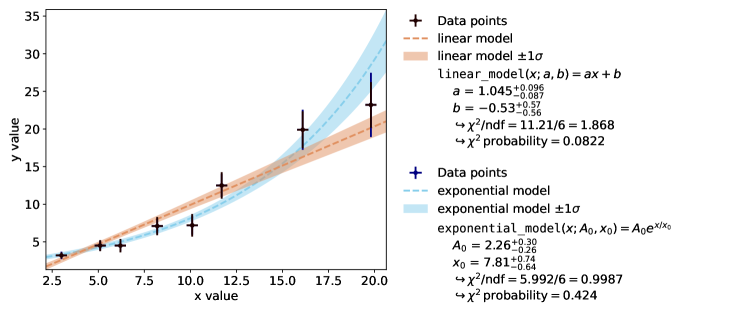
Figure 2: Fitting two models to the same data with kafe2.

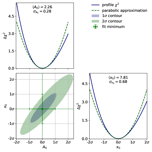
Figure 3: Two-dimensional confidence contours and profile likelihood curves for the exponential model.

The parameterization of the exponential model is - intentionally - chosen suboptimally to amplify the nonlinearity. The parameter $x_{0}$ is in the denominator of the expression in the exponent; if $x_{0}$ were replaced by a parameter $\lambda:=1/x_{0}$, then the parameter uncertainties derived from the Cramér-Rao-Fréchet bound would be more accurate. The deviation from the parabolic shape can be inspected via the profile likelihood curve, as shown in Figure 3. The profile likelihood for the parameter $x_{0}$ - drawn as a solid blue line - clearly deviates from the parabola that is extrapolated from the second derivative at the cost function minimum. The 68.3% confidence interval is determined by finding the intersection of the likelihood curves with a constant function equal to 1; the confidence interval derived from the profile likelihood method differs from the conventional confidence interval obtained by extrapolating the second derivatives. Instead of a symmetric uncertainty of $\pm$0.70, this results in an asymmetric confidence interval from -0.66 to +0.76 around the central value.

The exponential model is a linear function of the parameter $A_{0}$. Despite this, the profile likelihood of $A_{0}$ also differs from a parabola: the 68.3% confidence interval ranges from -0.27 to +0.32 relative to the central value. This effect is mostly caused by the relative uncertainties on the ordinate values, which are specified as relative to the model values. As such, larger model values increase the uncertainties and therefore result in a lower cost function value. Conversely, smaller model values result in a higher cost function value. The asymmetry of the uncertainty of parameter $a$ shown as the result of the linear fit in Figure 2 is caused by the same effect.

The third graph in the bottom left corner of Figure 3 shows the boundaries of the confidence regions for the shared distribution of $x_{0}$ and $A_{0}$, as determined by the profile likelihood method. The plot shows the confidence contours for $\Delta\chi^{2}=1$ and $\Delta\chi^{2}=4$, which correspond to the $1\,\sigma$ and $2\,\sigma$ uncertainty ranges, respectively. The slope of the contour reflects the strong correlation of 90% between the parameters $A_{0}$ and $x_{0}$. The cross indicates the uncertainties determined from the second derivatives at the minimum. The deviation from the elliptical shape is visible for both contours, but it is particularly pronounced for the $2\,\sigma$ contour. This is expected since the extrapolation of the second derivatives is more accurate close to the cost function minimum. Students should be encouraged to include the asymmetric uncertainties as well as the confidence contours when documenting their results.

4 Experiences and conclusion

The methods upon which kafe2 is built are a core part of the physics curriculum at the Karlsruhe Institute of Technology. Bachelor students are required to attend a lecture on computer-based data analysis which includes topics such as the basics of statistics and the visualization of data. The lecture is aimed at students in the second semester and serves as a preparation for the physics laboratory courses starting in the third semester. As such, the focus of the lecture is placed on equipping students with the tools and knowledge necessary to perform simple but modern data analyses on their own. More complex problems such as fits with user-defined maximum-likelihood functions or fits to histogram data arise in the context of advanced practical courses or work on projects done as part of a Bachelor’s thesis.

The kafe and kafe2 packages have been in continuous use at KIT in the context of physics laboratory courses since 2015. For ease of use, sample code is provided as part of a collection of useful Python functions for storage, processing and visualization (software package PhyPraKit [10]), which encapsulates the complex functionality of kafe2 and provides a simple interface sufficient for most practical needs. Optional tasks offer incentives to try out more complex functionality, replacing the traditional simple error calculation with complete uncertainty models with covariance matrix in the model fitting.

More in-depth lectures on data analysis that build on the foundations laid in the practical courses are offered to postgraduate students. Positive feedback from supervisors of Bachelor’s theses indicates that the students experience a significant gain in competence when it comes to the evaluation of scientific data as well as its visualization, discussion, and presentation in scientific contexts. The student surveys for the courses show that the prior knowledge in the area of digital data processing varies greatly from student to student. The acceptance of the tools provided, the assessment of their usefulness, and the positive awareness of the students’ own competence increase over the course of their studies.

The lecture on computer-based data analysis is deliberately placed early in the physics curriculum. Students can only experience a gain in knowledge from laboratory courses if they understand the mechanisms that the experiments are based on - this holds true both for the underlying physics and the statistical methods employed. However, the early introduction of software tools also necessitates that said tools are (comparatively) easy to use. Most physics students were taught at most basic programming in school and cannot be expected to learn how to apply the complex tools used in scientific practice. At the same time the available simple tools (some of which require no programming knowledge at all) do not use state-of-the-art statistical methods and thus cannot enlighten students when it is necessary to apply them. To brigde this gap, kafe2 aims to provide for an easy-to-use tool built on state-of-the-art statistical methods. While the early introduction of modern analysis methods still poses some difficulty, most students respond positively to the challenge and are ultimately able to master it well.

With the tools commonly used in basic physics education for model fitting and visualization, an analysis as shown in the examples above is practically impossible to perform. With kafe2, however, students have a sufficiently simple tool at their disposal to carry out data analysis tasks in accordance with contemporary scientific standards.

References

-
[1]
Description and source code kafe2,
URLs: https://philfitters.github.io/kafe2/ and https://github.com/PhiLFitters/kafe2/. - [2] Interpreted programming language Python, URL: https://www.python.org/.
-
[3]
Scientific computing library NumPy,
URL: https://numpy.org/,
Harris, C.R., Millman, K.J., van der Walt, S.J. et al., Array programming with NumPy, Nature 585, 357–362 (2020), DOI: 10.1038/s41586-020-2649-2. -
[4]
Graphics library matplotlib,
URL: https://matplotlib.org/,
J. D. Hunter, Matplotlib: A 2D Graphics Environment, Computing in Science & Engineering, vol. 9, no. 3, pp. 90-95, (2007), DOI: 10.5281/zenodo.7162185. -
[5]
Software library for mathematics, science and
engineering SciPy,
URL: https://www.scipy.org/,
Pauli Virtanen et al., SciPy 1.0: Fundamental Algorithms for Scientific Computing in Python, Nature Methods, 17(3), 261-272 (2020), DOI: 10.1038/s41592-019-0686-2. - [6] iminuit, URL: https://github.com/scikit-hep/iminuit/, Hans Dembinski, Piti Ongmongkolkul et al., DOI: 10.5281/zenodo.3949207.
- [7] Data analysis framework ROOT, URL: https://root.cern/.
- [8] Data description language YAML, URL: https://yaml.org/.
- [9] Interactive computing service Jupyter, URL: https://jupyter.org/.
-
[10]
Software package PhyPraKit for digital data processing
in physics laboratory courses,
URL: https://github.com/GuenterQuast/PhyPraKit/.