Multi-Objective GFlowNets

Abstract

We study the problem of generating diverse candidates in the context of Multi-Objective Optimization. In many applications of machine learning such as drug discovery and material design, the goal is to generate candidates which simultaneously optimize a set of potentially conflicting objectives. Moreover, these objectives are often imperfect evaluations of some underlying property of interest, making it important to generate diverse candidates to have multiple options for expensive downstream evaluations. We propose Multi-Objective GFlowNets (MOGFNs), a novel method for generating diverse Pareto optimal solutions, based on GFlowNets. We introduce two variants of MOGFNs: MOGFN-PC, which models a family of independent sub-problems defined by a scalarization function, with reward-conditional GFlowNets, and MOGFN-AL, which solves a sequence of sub-problems defined by an acquisition function in an active learning loop. Our experiments on wide variety of synthetic and benchmark tasks demonstrate advantages of the proposed methods in terms of the Pareto performance and importantly, improved candidate diversity, which is the main contribution of this work.

1 Introduction

Decision making in practical applications usually involves reasoning about multiple, often conflicting, objectives (Keeney et al., 1993). Consider the example of in-silico drug discovery, where the goal is to generate novel drug-like molecules that effectively inhibit a target, are easy to synthesize, and possess a safety profile for human use (Dara et al., 2021). These objectives often exhibit mutual incompatibility as molecules that are effective against a target may also have detrimental effects on humans, making it infeasible to find a single molecule that maximizes all the objectives simultaneously. Instead, the goal in these Multi-Objective Optimization (MOO; Ehrgott, 2005; Miettinen, 2012) problems is to identify candidate molecules that are Pareto optimal, covering the best possible trade-offs between the objectives.

A less appreciated aspect of multi-objective problems is that the objectives to optimize are usually underspecified proxies which only approximate the true design objectives. For instance, the binding affinity of a molecule to a target is an imperfect approximation of the molecule’s inhibitory effect against the target in the human body. In such scenarios it is important to not only cover the Pareto front but also to generate sets of diverse candidates for each Pareto optimal solution in order to increase the likelihood of success of the generated candidates in expensive downstream evaluations, such as in-vivo tests and clinical trials (Jain et al., 2022).

The benefits of generating diverse candidates are twofold. First, by diversifying the set of candidates we obtain an advantage similar to Bayesian ensembles: we reduce the risk of failure that might occur due to the imperfect generalization of learned proxy models. Diverse candidates should lie in different regions of the input-space manifold where the objective of interest might be large (considering the uncertainty in the output of the proxy model). Second, experimental measurements such as in-vitro assays may not reflect the ultimate objectives of interest, such as efficacy in human bodies. Multiple candidates may have the same assay score, but different downstream efficacy, so diversity in candidates increases odds of success. Existing approaches for MOO overlook this aspect of diversity and instead focus primarily on generating Pareto optimal solutions.

Generative Flow Networks (GFlowNets; Bengio et al., 2021a, b) are a recently proposed family of probabilistic models which tackle the problem of diverse candidate generation. Contrary to the reward maximization view of prevalent Reinforcement Learning (RL) and Bayesian optimization (BO) approaches, GFlowNets sample candidates with probability proportional to their reward. Sampling candidates, as opposed to greedily generating them implicitly encourages diversity in the generated candidates. GFlowNets have shown promising results in single objective problems such as molecule generation (Bengio et al., 2021a) and biological sequence design (Jain et al., 2022).

In this paper, we propose Multi-Objective GFlowNets (MOGFNs), which leverage the strengths of GFlowNets and existing MOO approaches to enable the generation of diverse Pareto optimal candidates. We consider two variants of MOGFNs – (a) Preference-Conditional GFlowNets (MOGFN-PC) which leverage the decomposition of MOO into single objective sub-problems through scalarization, and (b) MOGFN-AL, which leverages the transformation of MOO into a sequence of single objective sub-problems within the framework of multi-objective Bayesian optimization. Our contributions are as follows:

1. We introduce a novel framework of MOGFNs to tackle the practically significant and previously unexplored problem of diverse candidate generation in MOO.

2. Through experiments on challenging molecule generation and sequence generation tasks, we demonstrate that MOGFN-PC generates diverse Pareto-optimal candidates. This is the first successful application and empirical validation of reward-conditional GFlowNets (Bengio et al., 2021b).

3. In a challenging active learning task for designing fluorescent proteins, we show that MOGFN-AL results in significant improvements to sample efficiency as well as diversity of generated candidates.

4. We perform a thorough analysis on the key components of MOGFNs to provide insights into design choices that affect performance.

2 Background

2.1 Multi-Objective Optimization

Multi-objective Optimization (MOO) involves finding a set of feasible candidates $x^{\star}\in\mathcal{X}$ which simultaneously maximize $d$ objectives $\mathbf{R}(x)=[R_{1}(x),\dots,R_{d}(x)]$:

$$\max_{x\in\mathcal{X}}\mathbf{R}(x).$$ (1)

When these objectives are conflicting, there is no single $x^{\star}$ which simultaneously maximizes all objectives. Consequently, MOO adopts the concept of Pareto optimality, which describes a set of solutions that provide optimal trade-offs among the objectives.

Given $x_{1},x_{2}\in\mathcal{X}$, $x_{1}$ is said to dominate $x_{2}$, written ($x_{1}\succ x_{2}$), iff $R_{i}(x_{1})\geq R_{i}(x_{2})\enspace\forall i\in\{1,\dots,d\}$ and $\exists k\in\{1,\dots,d\}$ such that $R_{k}(x_{1})>R_{k}(x_{2})$. A candidate $x^{\star}$ is Pareto-optimal if there exists no other solution $x^{\prime}\in\mathcal{X}$ which dominates $x^{\star}$. In other words, for a Pareto-optimal candidate it is impossible to improve one objective without sacrificing another. The Pareto set is the set of all Pareto-optimal candidates in $\mathcal{X}$, and the Pareto front is defined as the image of the Pareto set in objective-space.

Diversity:

Since the objectives are not guaranteed to be injective, any point on the Pareto front can be the image of several candidates in the Pareto set. This designates diversity in candidate space. Capturing all the diverse candidates, corresponding to a point on the Pareto front, is critical for applications such as in-silico drug discovery, where the objectives $R_{i}$ (e.g. binding affinity to a target protein) are mere proxies for the more expensive downstream measurements (e.g., effectiveness in clinical trials on humans). This notion of diversity of candidates is typically not captured by existing approaches for MOO.

2.1.1 Approaches for tackling MOO

While, there exist many approaches tackling MOO problems (Ehrgott, 2005; Miettinen, 2012; Pardalos et al., 2017), in this work, we consider two distinct approaches that decompose the MOO problem into a family of single objective sub-problems. These approaches, described below, are well-suited for the GFlowNet formulations we introduce in Section 3.

Scalarization:

In scalarization, a set of weights (preferences) $\omega_{i}$ are assigned to the objectives $R_{i}$, where $\omega_{i}\geq 0$ and $\sum_{i=1}^{d}\omega_{i}=1$. The MOO problem can then be decomposed into single-objective sub-problems of the form $\max_{x\in\mathcal{X}}R(x|\omega)$, where $R(x|\omega)$ is called a scalarization function, which combines the $d$ objectives into a scalar. Solutions to these sub-problems capture all Pareto-optimal solutions to the original MOO problem depending on the choice of $R(x|\omega)$ and characteristics of the Pareto front. Weighted Sum Scalarization, $R(x|\omega)=\sum_{i=1}^{d}\omega_{i}R_{i}(x)$, for instance, captures all Pareto optimal candidates for problems with a convex Pareto front (Ehrgott, 2005). On the other hand, Weighted Tchebycheff, $R(x|\omega)=\max\limits_{1\leq i\leq d}{\omega_{i}|R_{i}(x)-z_{i}^{\star}|}$, where $z_{i}^{\star}$ denotes an ideal value for objective $R_{i}$, captures all Pareto optimal solutions even for problems with a non-convex Pareto front (Choo & Atkins, 1983; Pardalos et al., 2017). As such, scalarization transforms the multi-objective optimization into a family of independent single-objective sub-problems.

Multi-Objective Bayesian Optimization:

In many applications, the objectives $R_{i}$ can be expensive to evaluate, thereby making sample efficiency essential. Multi-Objective Bayesian optimization (MOBO) (Shah & Ghahramani, 2016; Garnett, 2022) builds upon BO to tackle these scenarios. MOBO relies on a probabilistic model $\hat{f}$ which approximates the objectives $\mathbf{R}$ (oracles). $\hat{f}$ is typically a multi-task Gaussian Process (Shah & Ghahramani, 2016). Notably, as the model is Bayesian, it captures the epistemic uncertainty in the predictions due to limited data available for training, which can be used as a signal for prioritizing potentially useful candidates. The optimization is performed over $M$ rounds, where each round $i$ consists of fitting the surrogate model $\hat{f}$ on the data $\mathcal{D}_{i}$ accumulated from previous rounds, and using this model to generate a batch of $b$ candidates $\{x_{1},\dots,x_{b}\}$ to be evaluated with the oracles $\mathbf{R}$, resulting in $\mathcal{B}_{i}=\{(x_{1},y_{1}),\dots,(x_{b},y_{b})\}$. The evaluated batch $\mathcal{B}$ is then incorporated into the data for the next round $\mathcal{D}_{i+1}=\mathcal{D}_{i}\cup\mathcal{B}$. The batch of candidates in each round is generated by maximizing an acquisition function $a$ which combines the predictions from the surrogate model along with its epistemic uncertainty into a single scalar utility score. The acquisition function quantifies the utility of a candidate given the candidates evaluated so far. Effectively, MOBO decomposes the MOO into a sequence of single objective optimization problems of the form $\max_{\{x_{1},\dots,x_{b}\}\in 2^{\mathcal{X}}}a(\{x_{1},\dots,x_{b}\};\hat{f})$.

2.2 GFlowNets

GFlowNets (Bengio et al., 2021a, b) are a family of probabilistic models that learn a stochastic policy to generate compositional objects $x\in\mathcal{X}$, such as a graph describing a candidate molecule, through a sequence of steps, with probability proportional to their reward $R(x)$. If $R:\mathcal{X}\to\mathbb{R}^{+}$ has multiple modes then i.i.d samples from $\pi\propto R$ gives a good coverage of the modes of $R$, resulting in a diverse set of candidate solutions. The sequential construction of $x\in\mathcal{X}$ can be described as a trajectory $\tau\in{\mathcal{T}}$ in a weighted directed acyclic graph (DAG) $\mathcal{G}=\left(\mathcal{S},\mathcal{E}\right)$, starting from an empty object $s_{0}$ and following actions $a\in\mathcal{A}$ as building blocks. For example, a molecular graph may be sequentially constructed by adding and connecting new nodes or edges to the graph. Let $s\in\mathcal{S}$, or state, denote a partially constructed object. Transitions between states $s\xrightarrow[]{a}s^{\prime}\in\mathcal{E}$ indicate that action $a$ at state $s$ leads to state $s^{\prime}$. Sequences of such transitions form constructive trajectories.

The GFlowNet forward policy $P_{F}(-|s)$ is a distribution over the children of state $s$. An object $x$ can be generated by starting at $s_{0}$ and sampling a sequence of actions iteratively from $P_{F}$. Similarly, the backward policy $P_{B}(-|s)$ is a distribution over the parents of state $s$ and can generate backward trajectories starting at any terminal $x$, e.g., iteratively sampling from $P_{B}$ starting at $x$ shows a way $x$ could have been constructed. Let $\pi(x)$ be the marginal likelihood of sampling trajectories terminating in $x$ following $P_{F}$, and partition function $Z=\sum_{x\in\mathcal{X}}R(x)$. The learning problem solved by GFlowNets is to learn a forward policy $P_{F}$ such that the marginal likelihood of sampling any object $\pi(x)$ is proportional to its reward $R(x)$. In this paper we adopt the trajectory balance (TB; Malkin et al., 2022) learning objective. The trajectory balance objective learns $P_{F}(-|s;\theta),P_{B}(-|s;\theta),Z_{\theta}$ parameterized by $\theta$, which approximate the forward and backward policies and partition function such that $\pi(x)\approx\frac{R(x)}{Z},\enspace\forall x\in\mathcal{X}$. We refer the reader to Bengio et al. (2021b); Malkin et al. (2022) for a more thorough introduction to GFlowNets.

3 Multi-Objective GFlowNets

In this section, we introduce Multi-Objective GFlowNets (MOGFNs) to tackle the problem of diverse Pareto optimal candidate generation. The two MOGFN variants we discuss respectively exploit the decomposition of MOO problems into a family of independent single objective subproblems or a sequence of single objective sub-problems.

3.1 Preference-Conditional GFlowNets

As discussed in Section 2.1, given an appropriate scalarization function, candidates optimizing each sub-problem $\max_{x\in\mathcal{X}}R(x|\omega)$ correspond to a single point on the Pareto front. As the objectives are often imperfect proxies for some underlying property of interest we aim to generate diverse candidates for each sub-problem. One naive way to achieve this is by solving each independent sub-problem with a separate GFlowNet. However, this approach not only poses significant computational challenges in terms of training a large number of GFlowNets, but also fails to take advantage of the shared structure present between the sub-problems.

Reward-conditional GFlowNets (Bengio et al., 2021b) are a generalization of GFlowNets that learn a single conditional policy to simultaneously model a family of distributions associated with a corresponding family of reward functions. Let $\mathcal{C}$ denote a set of values $c$, with each $c\in\mathcal{C}$ inducing a unique reward function $R(x|c)$. We can define a family of weighted DAGs $\{\mathcal{G}_{c}=\left(\mathcal{S}_{c},\mathcal{E}\right),\enspace c\in\mathcal{C}\}$ which describe the construction of $x\in\mathcal{X}$, with conditioning information $c$ available at all states in $\mathcal{S}_{c}$. Having $c$ as input allows the policy to learn the shared structure across different values of $c$. We denote $P_{F}(-|s,c)$ and $P_{B}(-|s^{\prime},c)$ as the conditional forward and backward policies, $Z(c)=\sum_{x\in\mathcal{X}}R(x|c)$ as the conditional partition function and $\pi(x|c)$ as the marginal likelihood (given $c$) of sampling trajectories $\tau$ from $P_{F}$ terminating in $x$. The learning objective in reward-conditional GFlowNets is thus estimating $P_{F}(-|s,c)$ such that $\pi(x|c)\propto R(x|c)$. Exploiting the shared structure enables a single conditional policy (e.g., a neural net taking $c$ and $s$ as input and actions probabilities as outputs) to model the entire family of reward functions simultaneously. Moreover, the policy can generalize to values of $c$ not seen during training.

The MOO sub-problems possess a similar shared structure, induced by the preferences. Thus, we can leverage a single reward-conditional GFlowNet instead of a set of independent GFlowNets to model the sub-problems simultaneously. Formally, Preference-conditional GFlowNets (MOGFN-PC) are reward-conditional GFlowNets with the preferences $\omega\in\Delta^{d}$ over the set of objectives $\{R_{1}(x),\dots,R_{d}(x)\}$ as the conditioning variable. MOGFN-PC models the family of reward functions defined by the scalarization function $R(x|\omega)$. MOGFN-PC is a general approach and can accommodate any scalarization function, be it existing ones discussed in Section 2.1 or novel scalarization functions designed for a particular task. To illustrate this flexibility, we introduce the Weighted-log-sum (WL): $R(x|\omega)=\prod_{i=1}^{d}R_{i}(x)^{\omega_{i}}$ scalarization function. We hypothesize that the weighted sum in $\log$ space can potentially can help in scenarios where all objectives are to be optimized simultaneously, and the scalar reward from Weighted-Sum can be dominated by a single reward. The scalarization function is a key component for MOGFN-PC, and we further study the empirical impact of various scalarization functions in Section 6.

Training MOGFN-PC

The procedure to train MOGFN-PC, or any reward-conditional GFlowNet, closely follows that of a standard GFlowNet and is described in Algorithm 1. The objective is to learn the parameters $\theta$ of the forward and backward conditional policies $P_{F}(-|s,\omega;\theta)$ and $P_{B}(-|s^{\prime},\omega;\theta)$, and the log-partition function $\log Z_{\theta}(\omega)$ such that $\pi(x|\omega)\propto R(x|\omega)$. To this end, we consider an extension of the trajectory balance objective:

$$\mathcal{L}(\tau,\omega;\theta)=\left(\log\frac{Z_{\theta}(\omega)\prod_{s\rightarrow s^{\prime}\in\tau}P_{F}(s^{\prime}|s,\omega;\theta)}{R(x|\omega)\prod_{s\rightarrow s^{\prime}\in\tau}P_{B}(s|s^{\prime},\omega;\theta)}\right)^{2}.$$ (2)

One important component is the distribution $p(\omega)$ used to sample preferences during training. $p(\omega)$ influences the regions of the Pareto front that are captured by MOGFN-PC. In our experiments, we use a Dirichlet$(\alpha)$ to sample preferences $\omega$ which are encoded with thermometer encoding (Buckman et al., 2018) when input to the policy in some of the tasks. Following prior work, we apply an exponent $\beta$ for the reward $R(x|\omega)$, i.e. $\pi(x|\omega)\propto R(x|\omega)^{\beta}$. This incentivizes the policy to focus on the modes of $R(x|\omega)$, which is critical for generation of high reward diverse candidates. By changing $\beta$ we can trade-off the diversity for higher rewards. We study the impact of these choices empirically in Section 6.

MOGFN-PC and MOReinforce

MOGFN-PC is closely related to MOReinforce (Lin et al., 2021) in that both learn a preference-conditional policy to sample Pareto-optimal candidates. The key difference is the learning objective: MOReinforce uses a multi-objective variant of REINFORCE (Williams, 1992), whereas MOGFN-PC uses a preference-conditional GFlowNet objective (Equation 2). MOReinforce, given a preference $\omega$ will converge to generating a single candidate that maximizes $R(x|\omega)$. MOGFN-PC, on the other hand, samples from $R(x|\omega)$, resulting in generation of diverse candidates from the Pareto set according to the preferences specified by $\omega$. This ability to generate diverse Pareto optimal candidates is a key feature of MOGFN-PC, whose advantage is demonstrated empirically in Section 5.

3.2 Multi-Objective Active Learning with GFlowNets

In many applications, the objective functions of interest are often computationally expensive to evaluate. Consider the drug discovery scenario, where evaluating objectives such as the binding energy of a candidate molecule to a target even in imperfect simulations can take several hours. Sample efficiency, in terms of number of evaluations of the objective functions, is therefore critical.

We introduce MOGFN-AL which leverages GFlowNets to generate candidates in each round of a multi-objective Bayesian optimization loop. MOGFN-AL tackles MOO through a sequence of single-objective sub-problems defined by acquisition function $a$. MOGFN-AL is a multi-objective extension of GFlowNet-AL (Jain et al., 2022). Here, we apply MOGFN-AL for biological sequence design summarized in Algorithm 2 (Appendix A), building upon the framework proposed by Stanton et al. (2022). This problem was previously studied by Seff et al. (2019) and has connections to denoising autoencoders (Bengio et al., 2013).

In existing work applying GFlowNets for biological sequence design, the GFlowNet policy generates the sequences token-by-token (Jain et al., 2022). While this offers greater flexibility to explore the space of sequences, it can be prohibitively slow when the sequences are large. In contrast, we use GFlowNets to propose candidates at each round $i$ by generating mutations for existing candidates $x\in\hat{\mathcal{P}}_{i}$ where $\hat{\mathcal{P}}_{i}$ is the set of non-dominated candidates in $\mathcal{D}_{i}$. Given a sequence $x$, the GFlowNet, through a sequence of stochastic steps, generates a set of mutations $m=\{(l_{i},v_{i})\}_{i=1}^{T}$ where $l\in\{1,\dots,|x|\}$ is the location to be replaced and $v\in\mathcal{A}$ is the token to replace $x[l]$ while $T$ is the number of mutations. Let ${x^{\prime}}_{m}$ be the sequence resulting from mutations $m$ on sequence $x$. The reward for a set of sampled mutations for $x$ is the value of the acquisition function on ${x^{\prime}}_{m}$, $R(m,x)=a({x^{\prime}}_{m}|\hat{f})$. This mutation based approach scales better to tasks with longer sequences while still affording ample exploration in sequence space for generating diverse candidates. We demonstrate this empirically in Section 5.3.

4 Related Work

Evolutionary Algorithms (EA)

Traditionally, evolutionary algorithms such as NSGA-II have been widely used in various multi-objective optimization problems (Ehrgott, 2005; Konak et al., 2006; Blank & Deb, 2020). More recently, Miret et al. (2022) incorporated graph neural networks into evolutionary algorithms enabling them to tackle large combinatorial spaces. Unlike MOGFNs, evolutionary algorithms are required to solve each instance of a MOO from scratch rather than by amortizing computation during training in order to quickly generate solutions at run-time. Evolutionary algorithms, however, can be augmented with MOGFNs for generating mutations to improve efficiency, as in Section 3.2.

Multi-Objective Reinforcement Learning

MOO problems have also received significant interest in the RL literature (Hayes et al., 2022). Traditional approaches broadly consist of learning sets of Pareto-dominant policies (Roijers et al., 2013; Van Moffaert & Nowé, 2014; Reymond et al., 2022). Recent work has focused on extending Deep RL algorithms for multi-objective settings, e.g., with Envelope-MOQ (Yang et al., 2019), MO-MPO (Abdolmaleki et al., 2020, 2021) , and MOReinforce (Lin et al., 2021). A general shortcoming of RL-based approaches is their objective focuses on discovering a single mode of the reward function, and thus hardly generate diverse candidates, an issue that also persists in the multi-objective setting. In contrast, MOGFNs sample candidates proportional to the reward, implicitly resulting in diverse candidates.

Multi-Objective Bayesian Optimization (MOBO)

Bayesian optimization (BO) has been used in the context of MOO when the objectives are expensive to evaluate and sample efficiency is a key consideration. MOBO approaches consist of learning a surrogate model of the true objective functions, which is used to define an acquisition function such as expected hypervolume improvement (Emmerich et al., 2011; Daulton et al., 2020, 2021) and max-value entropy search (Belakaria et al., 2019), as well as scalarization-based approaches (Paria et al., 2020; Zhang & Golovin, 2020). Abdolshah et al. (2019) and Lin et al. (2022) study the MOBO problem in the setting with preferences over the different objectives. Stanton et al. (2022) proposed LaMBO, which uses language models in conjunction with BO for multi-objective sequence design problems. While recent work (Konakovic Lukovic et al., 2020; Maus et al., 2022) studies the problem of generating diverse candidates in the context of MOBO, it is limited to local optimization near Pareto-optimal candidates in low-dimensional continuous problems. As such, the key drawbacks of MOBO approaches are that they typically do not consider the need for diversity in generated candidates and that they mainly consider continuous low-dimensional state spaces. As we discuss in Section 3.2, MOBO approaches can be augmented with GFlowNets for diverse candidate generation in discrete spaces.

Other Approaches

Zhao et al. (2022) introduced LaMOO which tackles the MOO problem by iteratively splitting the candidate space into smaller regions, whereas Daulton et al. (2022) introduce MORBO, which performs BO in parallel on multiple local regions of the candidate space. Both these methods, however, are limited to continuous candidate spaces.

5 Empirical Results

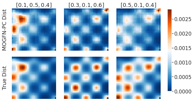
(a)

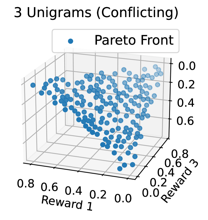
(b)

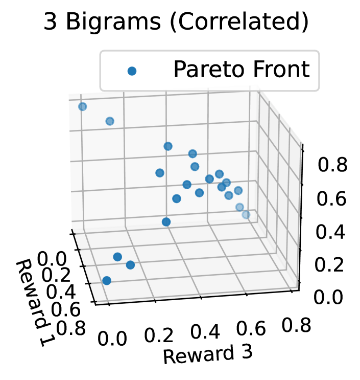
(c)

Figure 1: (a) The distribution learned by MOGFN-PC (Top) almost exactly matches the ground truth distribution (Bottom), in particular capturing all the modes, on hypergrid of size $32\times 32$ with 3 objectives. (b) and (c) Pareto front of candidates generated by MOGFN-PC on the N-grams task illustrates that the MOGFN-PC can model conflicting and correlated objectives well.

In this section, we present our empirical findings across a wide range of tasks ranging from sequence design to molecule generation. Through our experiments, we aim to answer the following questions:

1. Can MOGFNs model the preference-conditional reward distribution?

2. Can MOGFNs sample Pareto-optimal candidates?

3. Are candidates sampled by MOGFNs diverse?

4. Do MOGFNs scale to high-dimensional problems relevant in practice?

We obtain positive experimental evidence for Q1-Q4.

Metrics: We rely on standard MOO metrics such as the Hypervolume (HV) and $\bm{R}_{2}$ indicators, as well as the Generational Distance+ (GD+). To measure diversity we use the Top-K Diversity and Top-K Reward metrics of Bengio et al. (2021a). We detail all metrics in Appendix C. For all our empirical evaluations we follow the same protocol. First, we sample a set of preferences which are fixed for all the methods. For each preference we sample $128$ candidates from which we pick the top $10$, compute their scalarized reward and diversity, and report the averages over preferences. We then use these samples to compute the HV and $R_{2}$ indicators. We pick the best hyperparameters for all methods based on the HV and report the mean and standard deviation over $3$ seeds for all quantities.

Baselines: We consider the closely related MOReinforce (Lin et al., 2021) as a baseline. We also study its variants MOSoftQL and MOA2C which use Soft Q-Learning (Haarnoja et al., 2017) and A2C (Mnih et al., 2016) in place of REINFORCE. We additionally compare against Envelope-MOQ (Yang et al., 2019), another popular multi-objective reinforcement learning method. For fragment-based molecule generation we consider an additional baseline, MARS (Xie et al., 2021), a relevant MCMC approach for this task. Notably, we do not consider baselines like LaMOO (Zhao et al., 2022) and MORBO (Daulton et al., 2022) as they are designed for continuous spaces and rely on latent representations from pre-trained models for discrete tasks like molecule generation, making the comparisons unfair as the rest of the methods are trained on significantly fewer molecules. Additionally, it is not clear to apply them on tasks like DNA Aptamer design, where pretrained models are not available.

5.1 Synthetic Tasks

5.1.1 Hyper-Grid

We first study the ability of MOGFN-PC to capture the preference-conditional reward distribution in a multi-objective version of the HyperGrid task from Bengio et al. (2021a). The goal here is to navigate proportional to a reward within a HyperGrid. We consider the following objectives for our experiments: brannin(x), currin(x), shubert(x).

Since the state space is small, we can compute the distribution learned by MOGFN-PC in closed form. In Figure 1(a), we visualize $\pi(x|\omega)$, the distribution learned by MOGFN-PC conditioned on a set of fixed preference vectors $\omega$ and contrast it with the true distribution $R(x|\omega)$ in a $32\times 32$ hypergrid with 3 objectives. We observe that $\pi(-|\omega)$ and $R(-|\omega)$ are very similar. To quantify this, we compute $\mathbb{E}_{x}\left[|\pi(x|\omega)-R(x|\omega)/Z(\omega)|\right]$ averaged over a set of $64$ preferences, and find a difference of about $10^{-4}$. Note that MOGFN-PC is able to capture all the modes in the distribution, which suggests the candidates sampled from $\pi$ would be diverse. Further, we compute the GD+ metric for the Pareto front of candidates generated with MOGFN-PC, which comes up to an average value of 0.42. For more details about the task and the additional results, refer to Section D.1.

5.1.2 N-grams Task

We consider version of the synthetic sequence design task from Stanton et al. (2022). The task consists of generating strings with the objectives given by occurrences of a set of $d$ n-grams. MOGFN-PC adequately models the trade-off between conflicting objectives in the 3 Unigrams task as illustrated by the Pareto front of generated candidates in Figure 1(b). For the 3 Bigrams task with correlated objectives (as there are common characters in the bigrams), Figure 1(c) demonstrates MOGFN-PC generates candidates which can simultaneously maximize multiple objectives. We refer the reader to Section D.2 for more task details and additional results with different number of objectives and varying sequence length. In the results summarized in Table 7 in the Appendix, MOGFN-PC outperforms the baselines in terms of the MOO metrics while generating diverse candidates. Note that as occurrences of n-grams is the reward, the diversity is limited by the performance, i.e. high scoring sequences will have lower diversity, explaining higher diversity of MOSoftQL. We also observe that the MOReinforce and Envelope-MOQ baselines struggle in this task potentially due to longer trajectories with sparse rewards.

5.2 Benchmark Tasks

5.2.1 QM9

We first consider a small-molecule generation task based on the QM9 dataset (Ramakrishnan et al., 2014). We generate molecules atom-by-atom and bond-by-bond with up to 9 atoms and use 4 reward signals. The main reward is obtained via a MXMNet (Zhang et al., 2020) proxy trained on QM9 to predict the HOMO-LUMO gap. The other rewards are Synthetic Accessibility (SA), a molecular weight target, and a molecular logP target. Rewards are normalized to be between 0 and 1, but the gap proxy can exceed 1, and so is clipped at 2. The preferences $\omega$ are input to the policy as is, without thermometer encoding as we find no significant difference between the two choices. We train the models with 1M molecules and present the results in Table 1, showing that MOGFN-PC outperforms all baselines in terms of Pareto performance and diverse candidate generation.

Table 1: Atom-based QM9 task: MOGFN-PC exceeds Diversity and Pareto performance on QM9 task with HUMO-LUMO gap, SA, QED and molecular weight objectives compared to baselines.

Algorithm	Reward ($\uparrow$)	Diversity ($\uparrow$)	HV ($\uparrow$)	$R_{2}$ ($\downarrow$)
Envelope QL	0.65$\pm$0.06	0.85$\pm$0.01	1.26$\pm$0.05	5.80$\pm$0.20
MOReinforce	0.57$\pm$0.12	0.53$\pm$0.08	1.35$\pm$0.01	4.65$\pm$0.03
MOA2C	0.61$\pm$0.05	0.39$\pm$0.28	1.16$\pm$0.08	6.28$\pm$0.67
MOGFN-PC	0.76$\pm$0.00	0.93$\pm$0.00	1.40$\pm$0.18	2.44$\pm$1.88

Table 2: Fragment-based Molecule Generation Task: Diversity and Pareto performance on the Fragment-based drug design task with sEH, QED, SA and molecular weight objectives.

Algorithm	Reward ($\uparrow$)	Diversity ($\uparrow$)	HV ($\uparrow$)	$R_{2}$ ($\downarrow$)
Envelope QL	0.70$\pm$0.10	0.15$\pm$0.05	0.74$\pm$0.01	3.51$\pm$0.10
MARS	–	–	0.85$\pm$0.008	1.94$\pm$0.03
MOReinforce	0.41$\pm$0.07	0.01$\pm$0.007	0$\pm$0	9.88$\pm$1.06
MOA2C	0.76$\pm$0.16	0.48$\pm$0.39	0.75$\pm$0.01	3.35$\pm$0.02
MOGFN-PC	0.89$\pm$0.05	0.75$\pm$0.01	0.90$\pm$0.01	1.86$\pm$0.08

5.2.2 Fragment-Based Molecule Generation

We evaluate our method on the fragment-based (Kumar et al., 2012) molecular generation task of Bengio et al. (2021a), where the task is to generate molecules by linking fragments to form a junction tree (Jin et al., 2020). The main reward function is obtained via a pretrained proxy, available from Bengio et al. (2021a), trained on molecules docked with AutodockVina (Trott & Olson, 2010) for the sEH target. The other rewards are based on Synthetic Accessibility (SA), drug likeness (QED), and a molecular weight target. We detail the reward construction in Section D.4. The preferences $\omega$ are input to the policy directly for this task as well. Similarly to QM9, we train MOGFN-PC to generate 1M molecules and report the results in Table 2. We observe that MOGFN-PC is consistently outperforming baselines not only in terms of HV and $R_{2}$, but also candidate diversity score. Note that we do not report reward and diversity scores for MARS, since the lack of preference conditioning would make it an unfair comparison.

5.2.3 DNA Sequence Generation

A practical example of a design problem where the GFlowNet graph is a tree is the generation of DNA aptamers, single-stranded nucleotide sequences that are popular in biological polymer design due to their specificity and affinity as sensors in crowded biochemical environments (Zhou et al., 2017; Corey et al., 2022; Yesselman et al., 2019; Kilgour et al., 2021). We generate sequences by adding one nucleobase (A, C, T or G) at a time, with a maximum length of 60 bases. We consider three objectives: the free energy of the secondary structure calculated with the software NUPACK (Zadeh et al., 2011), the number of base pairs and the inverse of the sequence length (to favour shorter sequences).

The results summarized in Table 3 indicate that MOReinforce achieves the best MOO performance. However, we note that it finds a quasi-trivial solution with the pattern GCGCGC... for most lengths, yielding low diversity. In contrast, MOGFN-PC obtains much better diversity and Top-K rewards with slightly lower Pareto performance. See Section D.5 for further discussion.

Table 3: DNA Sequence Design Task: Diversity and Pareto performance of various algorithms on DNA sequence generation task with free energy, number of base pairs and inverse sequence length objectives.

Algorithm	Reward ($\uparrow$)	Diversity ($\uparrow$)	HV ($\uparrow$)	$R_{2}$ ($\downarrow$)
Envelope-MOQ	0.238$\pm$0.042	0.0$\pm$0.0	0.163$\pm$0.013	5.657$\pm$0.673
MOReinforce	0.105$\pm$0.002	0.6178$\pm$0.209	0.629$\pm$0.002	1.925$\pm$0.003
MOSoftQL	0.446$\pm$0.010	32.130$\pm$0.542	0.163$\pm$0.014	5.565$\pm$0.170
MOGFN-PC	0.682$\pm$0.021	18.131$\pm$0.981	0.517$\pm$0.006	2.432$\pm$0.002

5.3 Active Learning

Finally, to evaluate MOGFN-AL, we consider the Proxy RFP task from Stanton et al. (2022), with the aim of discovering novel proteins with red fluorescence properties, optimizing for folding stability and solvent-accessible surface area. We adopt all the experimental details (described in Section D.6) from Stanton et al. (2022), using MOGFN-AL for candidate generation. In addition to LaMBO, we use a model-free (NSGA-2) and model-based EA from Stanton et al. (2022) as baselines. We observe in Figure 2(a) that MOGFN-AL results in significant gains to the improvement in Hypervolume relative to the initial dataset, in a given budget of black-box evaluations. In fact, MOGFN-AL is able to match the performance of LaMBO within about half the number of black-box evaluations.

Figure 2(b) illustrates the Pareto frontier of candidates generated with MOGFN-AL, which dominates the Pareto frontier of the initial dataset. As we the candidates are generated by mutating sequences in the existing Pareto front, we also highlight the sequences that are mutations of each seqeunce in the initial dataset with the same color. To quantify the diversity of the generated candidates we measure the average e-value from DIAMOND (Buchfink et al., 2021) between the initial Pareto front and the Pareto frontier of generated candidates. Table 2(c) shows that MOGFN-AL generates candidates that are more diverse than the baselines.

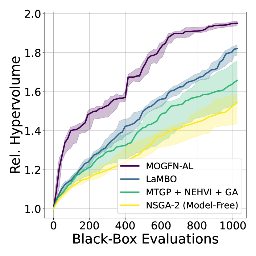
(a)

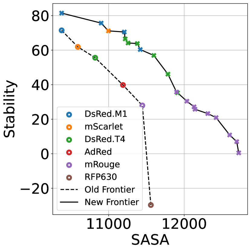
(b)

Algorithm	Diversity ($\uparrow$)
NSGA-2	0.07$\pm$0.03
MTGP + NEHVI + GA	0.12$\pm$0.02
LaMBO	0.18$\pm$0.03
MOGFN-AL	0.25$\pm$0.01

(c)

Figure 2: MOGFN-AL demonstrates a substantial advantage in terms of (a) Relative Hypervolume, and (b) the Pareto frontier of candidates generated by MOGFN-AL dominates the Pareto front of the initial dataset, while being more diverse (c) than the baselines’.

6 Analysis

In this section, we isolate the important components of MOGFN-PC: the distribution $p(\omega)$ for sampling preferences during training, the reward exponent $\beta$ and the scalarization function $R(x|\omega)$ to understand their impact on the performance. Figure 3 summarizes the results of the analysis on the 3 Bigrams task (Section 5.1.2) and the fragment-based molecule generation task (Section 5.2.1) with additional results in the Appendix B.

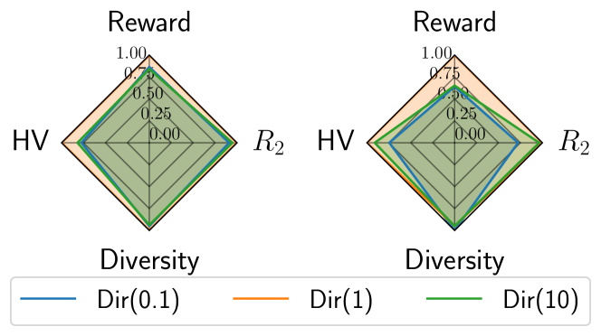
(a) $p(\omega)$

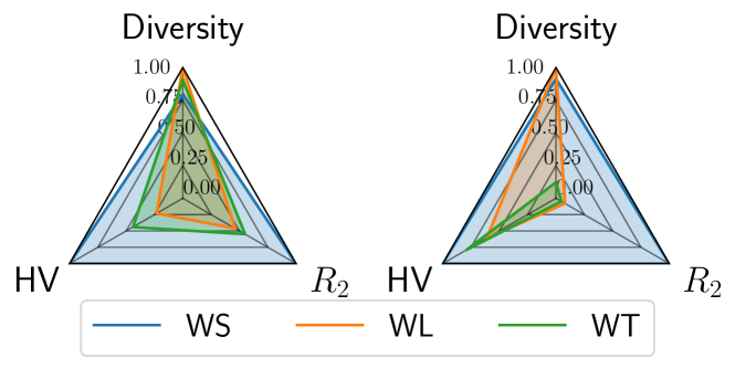
(b) $R(x|\omega)$

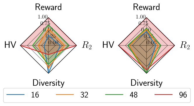
(c) $\beta$

Figure 3: Analysing the effect of $p(\omega)$, $R(x|\omega)$ and $\beta$ in the 3 Bigrams (left) and fragment-based molecule generation (right) tasks. The metrics are normalized by the maximum value obtained. As key takeaways, Dirichlet($\alpha=1$) for $p(\omega)$ and weighted sum (WS) scalarization have the best performance in both tasks while the choice of $\beta$ is task-dependent.

Impact of $p(\omega)$.

To examine the effect of $p(\omega)$, which controls the coverage of the Pareto front, we set it to $\text{Dirichlet}(\alpha)$ and vary $\alpha\in\{0.1,1,10\}$. This results in $\omega$ being sampled from different regions of $\Delta^{d}$. Specifically, $\alpha=1$ corresponds to a uniform distribution over $\Delta^{d}$, $\alpha>1$ is skewed towards the center of $\Delta^{d}$ whereas $\alpha<1$ is skewed towards the corners of $\Delta^{d}$. In Figure 3(a) we observe that $\alpha=1$ results in the best performance. Despite the skewed distribution with $\alpha=0.1$ and $\alpha=10$, we still achieve performance close to that of $\alpha=1$ indicating that MOGFN-PC is able to interpolate to preferences not sampled during training.

Choice of scalarization $R(x|\omega)$.

The set of $R(x|\omega)$ for different $\omega$ specifies the family of MOO sub-problems and thus has a critical impact on the Pareto performance. Figure 3(b) illustrates results for the Weighted Sum (WS), Weighted-log-sum (WL) and Weighted Tchebycheff (WT) scalarizations. Note that we do not compare the Top-K Reward as different scalarizations cannot be compared directly. WS scalarization results in the best performance. We suspect the poor performance of WT and WL are in part also due to the less smooth reward landscapes they induce.

Impact of $\beta$.

During training, $\beta$ controls the concentration of the reward density around modes of the distribution. For large values of $\beta$, the reward density around the modes become more peaky and vice-versa. In Figure 3(c) we present the results obtained by varying $\beta\in\{16,32,48,96\}$. As $\beta$ increases, MOGFN-PC is incentivized to generate samples closer to the modes of $R(x|\omega)$, resulting in better Pareto performance. However, with high $\beta$ values, the reward density is concentrated close to the modes and there is a negative impact on the diversity of the candidates. High values of $\beta$ also make the optimization harder, resulting in poorer performance. As such $\beta$ is a task specific parameter which can be tuned to identify the best trade-off between Pareto performance and diversity but also affects training efficiency.

7 Conclusion

In this work, we study Multi-Objective GFlowNets (MOGFN) for the generation of diverse Pareto-optimal candidates. We present two instantiations of MOGFNs: MOGFN-PC, which models a family of independent single-objective sub-problems with conditional GFlowNets, and MOGFN-AL, which optimizes a sequence of single-objective sub-problems. We demonstrate the efficacy of MOGFNs empirically on wide range of tasks ranging from molecule generation to protein design.

As a limitation, we note that the benefits of MOGFNs are limited in problems where the rewards have a single mode (see Section 5.2.3). For certain practical applications, we are interested only in a specific region of the Pareto front. Future work may explore gradient-based techniques to learn $p(\omega)$ for more structured exploration of the preference space. Within the context of MOFGN-AL, an interesting research avenue is the development of preference-conditional acquisition functions.

Code

The code for the experiments is available at https://github.com/GFNOrg/multi-objective-gfn.

Appendix A Algorithms

We summarize the algorithms for MOGFN-PC and MOGFN-AL here.

  Input:

  $p(\omega)$: Distribution for sampling preferences 

  $\beta$: Reward Exponent 

  $\delta$: Mixing Coefficient for uniform actions in sampling policy 

  $N$: Number of training steps 

  Initialize:$\left(P_{F}(s^{\prime}|s,\omega),P_{B}(s|s^{\prime},\omega),\log Z(\omega)\right)$: Conditional GFlowNet with parameters $\theta$ 

  for $i=1\enspace\text{to}\enspace N$ do

     Sample preference $\omega\sim p(\omega)$ 

     Sample trajectory $\tau$ following policy $\hat{\pi}=(1-\delta)P_{F}\enspace+\delta\text{Uniform}$  

     Compute reward $R(x|\omega)^{\beta}$ for generated samples and corresponding loss $\mathcal{L}(\tau,\omega;\theta)$ as in Equation 2 

     Update parameters $\theta$ with gradients from the loss, $\nabla_{\theta}\mathcal{L}(\tau,\omega)$ 

  end for

Algorithm 1 Training preference-conditional GFlowNets

  Input:

  $\mathbf{R}=\{R_{1},\dots,R_{d}\}$: Oracles to evaluate candidates $x$ and return true objectives $(R_{1}(x),\dots,R_{d}(x))$  

  $D_{0}=\{(x_{i},y_{i})\}$: Initial dataset with $y_{i}=\mathbf{R}(x_{i})$ 

  $\hat{f}$: Probabilistic surrogate model to model posterior over $\mathbf{R}$ given a dataset $\mathcal{D}$ 

  $a(x|\hat{f})$: Acquisition function computing a scalar utility for $x$ given $\hat{f}$ 

  $\pi_{\theta}$: Learnable GFlowNet policy 

  $b$: Size of candidate batch to be generated 

  $N$: Number of active learning rounds 

  Initialize:$\hat{f},\pi_{\theta}$ 

  for $i=1\enspace\text{to}\enspace M$ do

     Fit $\hat{f}$ on dataset $D_{i-1}$ 

     Extract the set of non-dominated candidates $\hat{\mathcal{P}}_{i-1}$ from $D_{i-1}$ 

     Train $\pi_{\theta}$ with to generate mutations for $x\in\hat{\mathcal{P}}_{i}$ using $a(-|\hat{f})$ as the reward 

     Generate batch $\mathcal{B}=\{x^{\prime}_{1,m_{i}},\ldots,x^{\prime}_{b,m_{b}}\}$ by sampling $x^{\prime}_{i}$ from $\hat{\mathcal{P}}_{i-1}$ and applying to it mutations $m_{i}$ sampled from $\pi_{\theta}$ 

     Evaluate batch $\mathcal{B}$ with $\mathbf{R}$ to generate $\hat{D}_{i}=\{(x_{1},\mathbf{R}(x_{1})),\ldots,(x_{b},\mathbf{R}(x_{b}))\}$ 

     Update dataset $D_{i}=\hat{D}_{i}\cup D_{i-1}$ 

  end for

  Result:Approximate Pareto set $\hat{\mathcal{P}}_{N}$

Algorithm 2 Training MOGFN-AL

Appendix B Additional Analysis

Can MOGFN-PC match Single Objective GFNs?

To evaluate how well MOGFN-PC models the family of rewards $R(x|\omega)$, we consider a comparison with single objective GFlowNets. More specifically, we first sample a set of 10 preferences ${\omega_{1},\dots,\omega_{10}}$, and train a standard single objective GFlowNet using the weighted sum scalar reward for each preference. We then generate $N=128$ candidates from each GFlowNet, throughout training, and compute the mean reward for the top 10 candidates for each preference. We average this top 10 reward across $\{\omega_{1},\dots,\omega_{10}\}$, and call it $R_{so}$. We then train MOGFN-PC, and apply the sample procedure with the preferences $\{\omega_{1},\dots,\omega_{10}\}$, and call the resulting mean of top 10 rewards $R_{mo}$. We plot the value of the ratio $R_{mo}/R_{so}$ in Figure 4. We observe that the ratio stays close to 1, indicating that MOGFN-PC can indeed model the entire family of rewards simultaneously at least as fast as a single objective GFlowNet could.

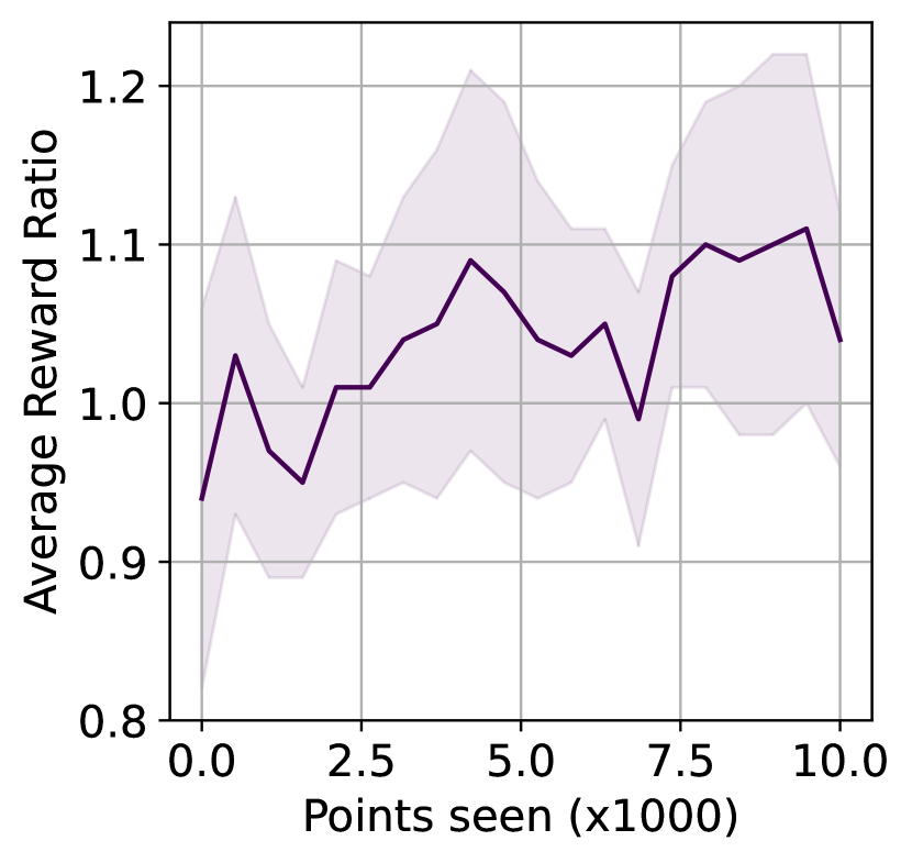
(a) 3 Bigrams task

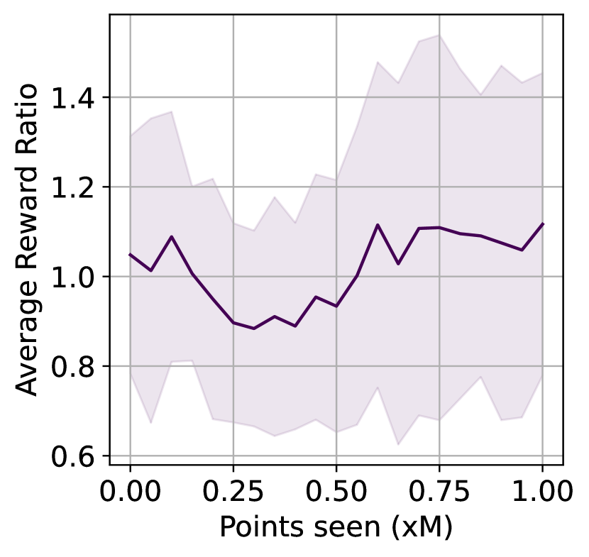
(b) Fragment-based Molecule Generation Task

Figure 4: We plot the ratio of rewards $R_{mo}/R_{so}$ for candidates generated with MOGFN-PC ($R_{m}o$) and single-objective GFlowNets($R_{so})$ for a set of preferences in the (a) 3 Bigrams and (b) Fragment-based molecule generation tasks. We observe that MOGFN-PC matches and occasionally surpasses single objective GFlowNets

Effect of Model Capacity and Architecture

Finally we look at the effect of model size in training MOGFN-PC. As MOGFN-PC models a conditional distribution, an entire family of functions as we’ve described before, we expect capacity to play a crucial role since the amount of information to be learned is higher than for a single-objective GFN. We increase model size in the 3 Bigrams task to see that effect, and see in Table 4 that larger models do help with performance–although the performance plateaus after a point. We suspect that in order to fully utilize the model capacity we might need better training objectives.

Table 4: Analysing the impact of model size on the performance of MOGFN-PC. Each architecture choice for the policy is denoted as A-B-C where A is number of layers, B is the number of hidden units in each layer, and C is the number of attention heads.

Metrics	Effect of model size
	3-64-8	3-256-8	4-64-8	4-256-8
Reward ($\uparrow$)	0.44$\pm$0.01	0.47$\pm$0.00	0.49$\pm$0.03	0.51$\pm$0.01
Diversity ($\uparrow$)	19.79$\pm$0.08	17.13$\pm$0.38	17.53$\pm$0.15	16.12$\pm$0.04
Hypervolume ($\uparrow$)	0.22$\pm$0.017	0.255$\pm$0.008	0.262$\pm$0.003	0.270$\pm$0.011
$R_{2}$ ($\downarrow$)	9.97$\pm$0.45	9.22$\pm$0.25	8.95$\pm$0.05	8.91$\pm$0.12

Appendix C Metrics

In this section we discuss the various metrics that we used to report the results in Section 5.

1. Generational Distance Plus (GD +) (Ishibuchi et al., 2015): This metric measures the euclidean distance between the solutions of the Pareto approximation and the true Pareto front by taking the dominance relation into account. To calculate GD+ we require the knowledge of the true Pareto front and hence we only report this metric for Hypergrid experiments (Section 5.1.1)

2. Hypervolume (HV) Indicator (Fonseca et al., 2006): This is a standard metric reported in Multi-Objective Optimization (MOO) works which measures the volume in the objective space with respect to a reference point spanned by a set of non-dominated solutions in Pareto front approximation.

3. $\bm{R}_{2}$ Indicator (Hansen & Jaszkiewicz, 1994): $R_{2}$ provides a monotonic metric comparing two Pareto front approximations using a set of uniform reference vectors and a utopian point $z^{*}$ representing the ideal solution of the MOO.

   This metric provides a monotonic reference to compare different Pareto front approximations relative to a utopian point. Specifically, we define a set of uniform reference vectors $\lambda\in\Lambda$ that cover the space of the MOO and then calculate:$R_{2}(\Gamma,\Lambda,z^{*})=\frac{1}{\lvert\Lambda\rvert}\sum_{\begin{subarray}{c}\lambda\in\Lambda\end{subarray}}\min_{\begin{subarray}{c}\gamma\in\Gamma\end{subarray}}\bigg{\{}\max_{\begin{subarray}{c}i\in{1,\ldots,k}\end{subarray}}\{\lambda_{i}\lvert z_{i}^{*}-\gamma_{i}\rvert\}\bigg{\}}$ where $\gamma\in\Gamma$ corresponds to the set of solutions in a given Pareto front approximations and $z^{*}$ is the utopian point corresponding to the ideal solution of the MOO. Generally, $R_{2}$ metric calculations are performed with $z^{*}$ equal to the origin and all objectives transformed to a minimization setting, which serves to preserve the monotonic nature of the metric. This holds true for our experiments as well.

4. Top-K Reward This metric was originally used in (Bengio et al., 2021a), which we extend for our multi-objective setting. For MOGFN-PC, we sample $N$ candidates per test preference and then pick the top-$k$ candidates ($k<N$) with highest scalarized rewards and calculate the mean. We repeat this for all test preferences enumerated from the simplex and report the average top-k reward score.

5. Top-K Diversity This metric was also originally used in (Bengio et al., 2021a), which we again extend for our multi-objective setting. We use this metric to quantify the notion of diversity of the generated candidates. Given a distance metric $d(x,y)$ between candidates $x$ and $y$ we calculate the diversity of candidates as those who have $d(x,y)$ greater than a threshold $\epsilon$. For MOGFN-PC, we sample $N$ candidates per test preference and then pick the top-k candidates based on the diversity scores and take the mean. We repeat this for all test preferences sampled from simplex and report the average top-k diversity score. We use the edit distance for sequences, and $1$ minus the Tanimoto similarity for molecules.

Appendix D Additional Experimental Details

D.1 Hyper-Grid

Here we elaborate on the Hyper-Grid experimental setup which we discussed in Section 5.1.1. Consider an $n$-dimensional hypercube gridworld where each cell in the grid corresponds to a state. The agent starts at the top left coordinate marked as $(0,0,\dots)$ and is allowed to move only towards the right, down, or stop. When the agent performs the stop action, the trajectory terminates and the agent receives a non-zero reward. In this work, we consider the following reward functions - brannin(x), currin(x), sphere(x), shubert(x), beale(x). In Figure 5, we show the heatmap for each reward function. Note that we normalize all the reward functions between 0 and 1.

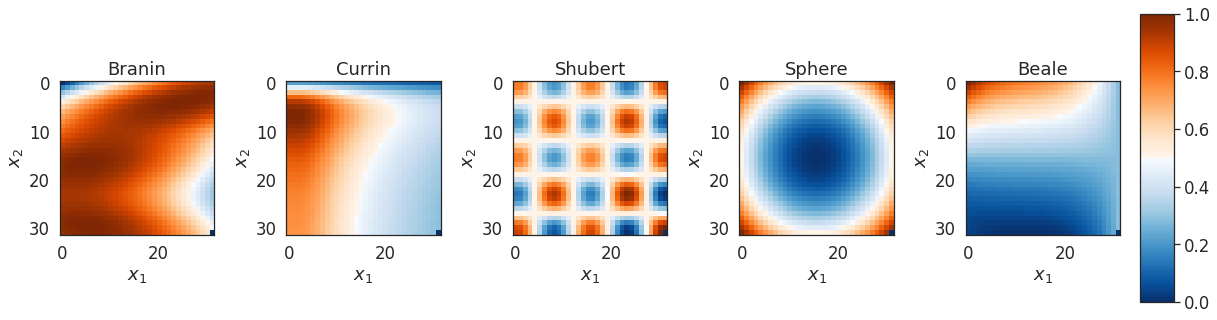
Figure 5: Reward Functions Different reward function considered for HyperGrid experiments presented in Section 5.1.1. Here the grid dimension is $H=32$

.

Additional Results To verify the efficacy of MOGFNs across different objectives sizes, we perform some additional experiments and measure the $L_{1}$ loss and the $GD+$ metric. In Figure 6, we can see that as the reward dimension increases, the loss and $GD+$ increases. This is expected because the number of rewards is indicative of the difficulty of the problem. We also present extended qualitative visualizations across more preferences in Figure 7.

Figure 6: (Left) Average test loss between the MOGFN-PC distribution and the true distribution for increasing number of objectives. (Right) GD $+$ metrics of MOGFN-PC across objectives.

Model Details and Hyperparameters For MOGFN-PC policies we use an MLP with two hidden layers each consisting of 64 units. We use LeakyReLU as our activation function as in (Bengio et al., 2021a). All models are trained with learning rate=0.01 with the Adam optimizer (Kingma & Ba, 2015) and batch size=128. We sample preferences $\omega$ from $\text{Dirichlet}(\alpha)$ where $\alpha=1.5$. We try two encoding techniques for encoding preferences - 1) Vanilla encoding where we just use the raw values of the preference vectors and 2) Thermometer encoding (Buckman et al., 2018). In our experiments we have not observed significant difference in performance difference.

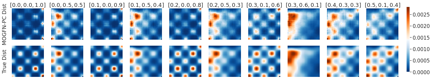
Figure 7: Extended Qualitative Visualizations for Hypergrid epxeriments

D.2 N-grams Task

Task Details The task is to generate sequences of some maximum length $L$, which we set to $36$ for the experiments in Section 5.1.2. We consider a vocabulary (actions) of size $21$, with $20$ characters ["A", "R", "N", "D", "C", "E", "Q", "G", "H", "I", "L", "K", "M", "F", "P", "S", "T", "W", "Y", "V"] and a special token to indicate the end of sequence. The rewards $\{R_{i}\}_{i=1}^{d}$ are defined by the number of occurrences of a given set of n-grams in a sequence $x$. For instance, consider ["AB", "BA"] as the n-grams. The rewards for a sequence $x=\texttt{ABABC}$ would be $[2,1]$. We consider two choices of n-grams: (a) Unigrams: the number of occurrences of a set of unigrams induces conflicting objectives since we cannot increase the number of occurrences of a monogram without replacing another in a string of a particular length, (b) Bigrams: given common characters within the bigrams, the occurrences of multiple bigrams can be increased simultaneously within a string of a fixed length. We also consider different sizes for the set of n-grams considered, i.e. different number of objectives. This allows us to evaluate the behaviour of MOGFN-PC on a variety of objective spaces. We summarize the specific objectives used in our experiments in Table 5. We normalize the rewards to $[0,1]$ in our experiments.

Table 5: Objectives considered for the N-grams task

Objectives	n-grams
2 Unigrams	["A", "C"]
2 Bigrams	["AC", "CV"]
3 Unigrams	["A", "C", "V"]
3 Bigrams	["AC", "CV", "VA"]
4 Unigrams	["A", "C", "V", "W"]
4 Bigrams	["AC", "CV", "VA", "AW"]

Model Details and Hyperparameters We build upon the implementation from Stanton et al. (2022) for the task: https://github.com/samuelstanton/lambo. For the string generation task, the backward policy $P_{B}$ is trivial (as there is only one parent for each node $s\in\mathcal{S}$), so we only have to parameterize $P_{F}$ and $\log Z$. As $P_{F}(-|s,\omega)$ is a conditional policy, we use a Conditional Transformer encoder as the architecture. This consists of a Transformer encoder (Vaswani et al., 2017) with 3 hidden layers of dimension $64$ and $8$ attention heads to embed the current state (string generated so far) $s$. We have an MLP which embeds the preferences $\omega$ which are encoded using thermometer encoding with $50$ bins. The embeddings of the state and preferences are concatenated and passed to a final MLP which generates a categorical distribution over the actions (vocabulary token). We use the same architecture for the baselines using a conditional policy – MOReinforce and MOSoftQL. For Envelope-MOQ, which does not condition on the preferences, we use a standard Transformer-encoder with a similar architecture. We present the hyperparameters we used in Table 6. Each method is trained for 10,000 iterations with a minibatch size of 128. For the baselines we adopt the official implementations released by the authors for MOReinforce – https://github.com/Xi-L/PMOCO and Envelope-MOQ – https://github.com/RunzheYang/MORL.

Table 6: Hyperparameters for N-grams Task

Hyperparameter	Values
Learning Rate ($P_{F}$)	{0.01, 0.05, 0.001, 0.005, 0.0001}
Learning Rate ($Z$)	{0.01, 0.05, 0.001}
Reward Exponent: $\beta$	{16, 32, 48}
Uniform Policy Mix: $\delta$	{0.01, 0.05, 0.1}

Additional Results

Table 7: N-Grams Task: Diversity and Pareto performance of various algorithms on for the 3 Bigrams and 3 Unigrams tasks with MOGFN-PC achieving superior Pareto performance.

Algorithm	3 Bigrams				3 Unigrams
	Reward ($\uparrow$)	Diversity ($\uparrow$)	HV ($\uparrow$)	$R_{2}$ ($\downarrow$)	Reward ($\uparrow$)	Diversity ($\uparrow$)	HV ($\uparrow$)	$R_{2}$ ($\downarrow$)
Envelope-MOQ	0.05$\pm$0.04	0$\pm$0	0.012$\pm$0.013	19.66$\pm$0.66	0.08$\pm$0.015	0$\pm$0	0.023$\pm$0.011	21.18$\pm$0.72
MOReinforce	0.12$\pm$0.02	0$\pm$0	0.015$\pm$0.021	20.32$\pm$0.93	0.03$\pm$0.001	0$\pm$0	0.036$\pm$0.009	21.04$\pm$0.51
MOSoftQL	0.28$\pm$0.03	21.09$\pm$0.65	0.093$\pm$0.025	15.79$\pm$0.23	0.36$\pm$0.01	23.131$\pm$0.6736	0.105$\pm$0.014	12.80$\pm$0.26
MOGFN-PC	0.44$\pm$0.01	19.79$\pm$0.08	0.220$\pm$0.017	9.97$\pm$0.45	0.38$\pm$0.00	22.71$\pm$0.24	0.121$\pm$0.015	11.39$\pm$0.17

We present some additional results for the n-grams task. First, Table 7 summarizes the numerical results for the experiments in subsubsection 5.1.2. Further, We consider different number of objectives $d\in\{2,4\}$ in Table 8 and Table 9 respectively. As with the experiments in Section 5.1.2 we observe that MOGFN-PC outperforms the baselines in Pareto performance while achieving high diversity scores. In Table 10, we consider the case of shorter sequences $L=24$. MOGFN-PC continues to provide significant improvements over the baselines. There are two trends we can observe considering the N-grams task holistically:

1. As the sequence size increases the advantage of MOGFN-PC becomes more significant.

2. The advantage of MOGFN-PC increases with the number of objectives.

Table 8: N-grams Task. 2 Objectives

Algorithm	2 Bigrams				2 Unigrams
	Reward ($\uparrow$)	Diversity ($\uparrow$)	HV ($\uparrow$)	$R_{2}$ ($\downarrow$)	Reward ($\uparrow$)	Diversity ($\uparrow$)	HV ($\uparrow$)	$R_{2}$ ($\downarrow$)
Envelope-MOQ	0.05$\pm$0.001	0$\pm$0	0.0$\pm$0.0	7.74$\pm$0.42	0.09$\pm$0.02	0$\pm$0	0.014$\pm$0.001	5.73$\pm$0.09
MOReinforce	0.12$\pm$0.01	0$\pm$0	0.151$\pm$0.023	0.031$\pm$	0.43$\pm$0.04	0$\pm$0	0.222$\pm$0.013	2.54$\pm$0.06
MOSoftQL	0.37$\pm$0.03	19.40$\pm$0.91	0.247$\pm$0.031	2.92$\pm$0.39	0.46$\pm$0.02	22.05$\pm$0.04	0.253$\pm$0.003	2.54$\pm$0.02
MOGFN-TB	0.51$\pm$0.04	20.65$\pm$0.58	0.321$\pm$0.011	2.31$\pm$0.04	0.48$\pm$0.01	22.15$\pm$0.22	0.267$\pm$0.007	2.24$\pm$0.03

Table 9: N-grams Task. 4 Objectives

Algorithm	4 Bigrams				4 Unigrams
	Reward ($\uparrow$)	Diversity ($\uparrow$)	HV ($\uparrow$)	$R_{2}$ ($\downarrow$)	Reward ($\uparrow$)	Diversity ($\uparrow$)	HV ($\uparrow$)	$R_{2}$ ($\downarrow$)
Envelope-MOQ	0$\pm$0	0$\pm$0	0$\pm$0	85.23$\pm$2.78	0$\pm$0	0$\pm$0	0$\pm$0	80.36$\pm$3.16
MOReinforce	0.01$\pm$0.00	0$\pm$0	0.001$\pm$0.001	60.42$\pm$1.52	0.00$\pm$0.00	0$\pm$0	0$\pm$0	79.12$\pm$4.21
MOSoftQL	0.12$\pm$0.04	24.32$\pm$1.21	0.013$\pm$0.001	39.31$\pm$1.35	0.22$\pm$0.02	24.18$\pm$1.43	0.019$\pm$0.005	31.46$\pm$2.32
MOGFN-TB	0.23$\pm$0.02	20.31$\pm$0.43	0.055$\pm$0.017	24.42$\pm$1.44	0.33$\pm$0.01	23.24$\pm$0.23	0.063$\pm$0.032	23.31$\pm$2.03

Table 10: N-grams Task. Shorter Sequences

Algorithm	3 Bigrams				3 Unigrams
	Reward ($\uparrow$)	Diversity ($\uparrow$)	HV ($\uparrow$)	$R_{2}$ ($\downarrow$)	Reward ($\uparrow$)	Diversity ($\uparrow$)	HV ($\uparrow$)	$R_{2}$ ($\downarrow$)
Envelope-MOQ	0.07$\pm$0.01	0$\pm$0	0.027$\pm$0.010	16.21$\pm$0.48	0.08$\pm$0.02	0$\pm$0	0.031$\pm$0.015	20.13$\pm$0.41
MOReinforce	0.18$\pm$0.01	0$\pm$0	0.053$\pm$0.031	13.35$\pm$0.82	0.07$\pm$0.02	0$\pm$0	0.041$\pm$0.009	19.25$\pm$0.41
MOSoftQL	0.31$\pm$0.02	20.12$\pm$0.51	0.143$\pm$0.019	12.79$\pm$0.41	0.38$\pm$0.02	21.13$\pm$0.35	0.109$\pm$0.011	12.12$\pm$0.24
MOGFN-PC	0.45$\pm$0.02	19.62$\pm$0.04	0.225$\pm$0.009	9.82$\pm$0.23	0.39$\pm$0.01	21.94$\pm$0.21	0.125$\pm$0.015	10.91$\pm$0.14

D.3 QM9

Reward Details As mentioned in Section 5.2.1, we consider four reward functions for our experiments. The first reward function is the HUMO-LUMO gap, for which we rely on the predictions of a pretrained MXMNet (Zhang et al., 2020) model trained on the QM9 dataset (Ramakrishnan et al., 2014). The second reward is the standard Synthetic Accessibility score which we calculate using the RDKit library (Landrum, ), to get the reward we compute $(10-\texttt{SA})/9$. The third reward function is molecular weight target. Here we first calculate the molecular weight of a molecule using RDKit, and then construct a reward function of the form $e^{-(\texttt{molWt}-105)^{2}/150}$ which is maximized at 105. Our final reward function is a logP target, $e^{-(\texttt{logP}-2.5)^{2}/2}$, which is again calculated with RDKit and is maximized at 2.5.

Model Details and Hyperparameters We sample new preferences for every episode from a $Dirichlet(\alpha)$, and encode the desired sampling temperature using a thermometer encoding (Buckman et al., 2018). We use a graph neural network based on a graph transformer architecture (Yun et al., 2019). We transform this conditional encoding to an embedding using an MLP. The embedding is then fed to the GNN as a virtual node, as well as concatenated with the node embeddings in the graph. The model’s action space is to add a new node to the graph, a new bond, or set node or bond properties (like making a bond a double bond). It also has a stop action. For more details please refer to the code provided in the supplementary material. We summarize the hyperparameters used in Table 11.

Hyperparameter	Value
Learning Rate ($P_{F}$)	0.0005
Learning Rate ($Z$)	0.0005
Reward Exponent: $\beta$	32
Batch Size:	64
Number of Embeddings	64
Uniform Policy Mix: $\delta$	0.001
Number of layers	4

Table 11: Hyperparameters for QM9 Task

D.4 Fragments

More Details As mentioned in Section 5.2.2, we consider four reward functions for our experiments. The first reward function is a proxy trained on molecules docked with AutodockVina (Trott & Olson, 2010) for the sEH target; we use the weights provided by Bengio et al. (2021a). We also use synthetic accessibility, as for QM9, and a weight target region (instead of the specific target weight used for QM9), ((300 - molwt) / 700 + 1).clip(0, 1) which favors molecules with a weight of under 300. Our final reward function is QED which is again calculated with RDKit.

Model Details and Hyperparameters We again use a graph neural network based on a graph transformer architecture (Yun et al., 2019). The experimental protocol is similar to QM9 experiments discussed in Section D.3. We additionally sample from a lagged model whose parameters are updated as $\theta^{\prime}=\tau\theta^{\prime}+(1-\tau)\theta$. The model’s action space is to add a new node, by choosing from a list of fragments and an attachment point on the current molecular graph. We list all hyperparameters used in Table 12.

Hyperparameter	Value
Learning Rate ($P_{F}$)	0.0005
Learning Rate ($Z$)	0.0005
Reward Exponent: $\beta$	96
Batch Size:	256
Sampling model $\tau$	0.95
Number of Embeddings	128
Number of layers	6

Table 12: Hyperparameters for Fragments

Additional Results We also present in Figure 8 a view of the reward distribution produced by MOGFN-PC. Generally, the model is able to find good near-Pareto-optimal samples, but is also able to spend a lot of time exploring. The figure also shows that the model is able to respect the preference conditioning, and remains capable of generating a diverse distribution rather than a single point.

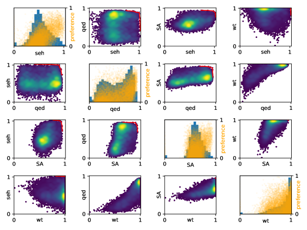
Figure 8: Fragment-based molecule generation: See Section D.4.

In the off-diagonal plots of Figure 8, we show pairwise scatter plots for each objective pair; the Pareto front is depicted with a red line; each point corresponds to a molecule generated by the model as it explores the state space; color is density (linear viridis palette). The diagonal plots show two overlaid informations: a blue histogram for each objective, and an orange scatter plot showing the relationship between preference conditioning and generated molecules. The effect of this conditioning is particularly visible for seh (top left) and wt (bottom right). As the preference for the sEH binding reward gets closer to 1, the generated molecules’ reward for sEH gets closer to 1 as well. Indeed, the expected shape for such a scatter plot is a triangular-ish shape: when the preference $\omega_{i}$ for reward $R_{i}$ is close to 1, the model is expected to generate objects with a high reward for $R_{i}$; as the preference $\omega_{i}$ gets further away from 1, the model can generate anything, including objects with a high $R_{i}$–that is, unless there is a trade off between objectives, in which case in cannot; this is the case for the seh objective, but not for the wt objective, which has a more triangular shape.

D.5 DNA Sequence Design

Task Details

The set of building blocks here consists of the bases["A", "C", "T", "G"] in addition to a special end of sequence token. In order to compute the free energy and number of base with the software NUPACK (Zadeh et al., 2011), we used 310 K as the temperature. The inverse of the length $L$ objective was calculated as $\frac{30}{L}$, as 30 was the minimum length for sampled sequences. The rewards are normalized to $[0,1]$ for our experiments.

Model Details and Hyperparameters

We use the same implementation as the N-grams task, detailed in Section D.2. Here we consider a 4-layer Transformer architecture, with 256 units per layer and $16$ attention head instead. We detail the most relevant hyperparameters Table 13.

Table 13: Hyperparameters tuned for DNA-Aptamers Task.

Hyperparameter	Values
Learning Rate ($P_{F}$)	{0.001, 0.0001, 0.00001, 0.000001}
Learning Rate ($Z$)	0.001
Reward Exponent: $\beta$	{40, 60, 80}
Batch Size:	16
Training iterations:	10,000
Dirichlet $\alpha$	{0.1, 1.0, 1.5}

Discussion of Results

Contrary to the other tasks on which we evaluated MOGFN-PC, for the generation of DNA aptamer sequences, our proposed model did not match the best baseline, multi-objective reinforcement learning (Lin et al., 2021), in terms of Pareto performance. Nonetheless, it is worth delving into the details in order to better understand the different solutions found by the two methods. First, as indicated in Section 5, despite the better Pareto performance, the best sequences generated by the RL method have extremely low diversity (0.62), compared to MOGFN, which generates optimal sequences with diversity of 19.6 or higher. As a matter of fact, MOReinforce mostly samples sequences with the well-known pattern GCGC... for all possible lengths. Sequences with this pattern have indeed low (negative) energy and many number of pairs, but they offer little new insights and poor diversity if the model is not able to generate sequences with other distinct patterns. On the contrary, GFlowNets are able to generate sequences with patterns other than repeating the pair of bases G and C. Interestingly, we observed that GFlowNets were able to generate sequences with even lower energy than the best sequences generated by MOReinforce by inserting bases A and T into chains of GCGC.... Finally, we observed that one reason why MOGFN does not match the Pareto performance of MOReinforce is because for short lengths (one of the objectives) the energy and number of pairs are not successfully optimised. Nonetheless, the optimisation of energy and number of pairs is very good for the longest sequences. Given these observations, we conjecture that there is room for improving the set of hyperparameters or certain aspects of the algorithm.

Additional Results

In order to better understand the impact of the main hyperparameters of MOGFN-PC in the Pareto performance and diversity of the optimal candidates, we train multiple instances by sweeping over several values of the hyperparameters, as indicated in Table 13. We present the results in Table 14. One key observation is that there seems to be a tradeoff between the Pareto performance and the diversity of the Top-K sequences. Nonetheless, even the models with the lowest diversity are able to generate much more diverse sequences than MOReinforce. Furthermore, we also observe $\alpha<1$ as the parameter of the Dirichlet distribution to sample the weight preferences, as well as higher $\beta$ (reward exponent), both yield better metrics of Pareto performance but slightly worse diversity. In the case of $\beta$, this observation is consistent with the results of the analysis in the Bigrams task (Figure 3), but with Bigrams, best performance was obtained with $\alpha=1$. This is indicative of a degree of dependence on the task and the nature of the objectives.

Table 14: Analysis of the impact of $\alpha$, $\beta$ and the learning rate on the performance of MOGFN-PC for DNA sequence design. We observe a trade-off between the Top-K diversity and the Pareto performance.

Metrics	Effect of $p(\omega)$			Effect of $\beta$			Effect of the learning rate
	Dir($\alpha=0.1$)	Dir($\alpha=1$)	Dir($\alpha=1.5$)	40	60	80	$10^{-5}$	$10^{-4}$	$10^{-3}$	$10^{-2}$
Reward ($\uparrow$)	0.687$\pm$0.01	0.652$\pm$0.01	0.639$\pm$0.01	0.506$\pm$0.01	0.560$\pm$0.01	0.652$\pm$0.01	0.587$\pm$0.01	0.652$\pm$0.01	0.654$\pm$0.03	0.604$\pm$0.01
Diversity ($\uparrow$)	17.65$\pm$0.37	19.58$\pm$0.15	20.18$\pm$0.58	28.49$\pm$0.32	24.93$\pm$0.19	19.58$\pm$0.15	21.92$\pm$0.59	19.58$\pm$0.15	19.51$\pm$1.14	23.16$\pm$0.18
Hypervolume ($\uparrow$)	0.506$\pm$0.01	0.467$\pm$0.02	0.440$\pm$0.01	0.277$\pm$0.03	0.363$\pm$0.03	0.467$\pm$0.02	0.333$\pm$0.01	0.467$\pm$0.02	0.496$\pm$0.01	0.336$\pm$0.01
$R_{2}$ ($\downarrow$)	2.462$\pm$0.05	2.576$\pm$0.08	2.688$\pm$0.02	4.225$\pm$0.34	2.905$\pm$0.18	2.576$\pm$0.08	3.855$\pm$0.31	2.576$\pm$0.01	2.488$\pm$0.03	3.422$\pm$0.07

D.6 Active Learning

Task Details We consider the Proxy RFP task from Stanton et al. (2022), an in silico benchmark task designed to simulate searching for improved red fluorescent protein (RFP) variants (Dance et al., 2021). The objectives considered are stability (-dG or negative change in Gibbs free energy) and solvent-accessible surface area (SASA) (Shrake & Rupley, 1973) in simulation, computed using the FoldX suite (Schymkowitz et al., 2005) and BioPython (Cock et al., 2009). We use the dataset introduced in Stanton et al. (2022) as the initial pool of candidates $\mathcal{D}_{0}$ with $|\mathcal{D}_{0}|=512$.

Method Details and Hyperparameters Our implementation builds upon the publicly released code from (Stanton et al., 2022): https://github.com/samuelstanton/lambo. We follow the exact experimental setup used in (Stanton et al., 2022). The surrogate model $\hat{f}$ consists of an encoder with 1D convolutions (masking positions corresponding to padding tokens). We used $3$ standard pre-activation residual blocks with two convolution layers, layer norm, and swish activations, with a kernel size of 5, 64 intermediate channels and 16 latent channels. A multi-task GP with an ICM kernel is defined in the latent space of this encoder, which outputs the predictions for each objective. We also use the training tricks detailed in Stanton et al. (2022) for the surrogate model. The hyperparameters, taken from Stanton et al. (2022) are shown in Table 15. The acquisiton function used is NEHVI (Daulton et al., 2021) defined as

$$\alpha(\{x_{j}\}_{j=1}^{i})=\frac{1}{N}\sum_{t=1}^{N}\text{HVI}(\{\tilde{f}_{t}(x_{j})\}_{j=1}^{i-1}|\mathcal{P}_{t})+\frac{1}{N}\sum_{t=1}^{N}\text{HVI}(\tilde{f}_{t}(x_{j})|\mathcal{P}_{t}\cup\{\tilde{f}_{t}(x_{j})\}_{j=1}^{i-1})$$ (3)

where $\tilde{f}_{t},t={1,\dots N}$ are independent draws from the surrogate model (which is a posterior over functions), and $\mathcal{P}_{t}$ denotes the Pareto frontier in the current dataset $\mathcal{D}$ under $\tilde{f}_{t}$.

Table 15: Hyperparameters for training the surrogate model $\hat{f}$

Hyperparameter	Value
Shared enc. depth (# residual blocks)	3
Disc. enc. depth (# residual blocks)	1
Decoder depth (# residual blocks)	3
Conv. kernel width (# tokens)	5
# conv. channels	64
Latent dimension	16
GP likelihood variance init	0.25
GP lengthscale prior	N(0.7, 0.01)
# inducing points (SVGP head)	64
DAE corruption ratio (training)	0.125
DAE learning rate (MTGP head)	5.00E-03
DAE learning rate (SVGP head)	1.00E-03
DAE weight decay	1.00E-04
Adam EMA params	0., 1e-2
Early stopping holdout ratio	0.1
Early stopping relative tolerance	1.00E-03
Early stopping patience (# epochs)	32
Max # training epochs	256

We replace the LaMBO candidate generation with GFlowNets. We generate a set of mutations $m=\{(l_{i},v_{i})\}$ for a sequences $x$ from the current approximation of the Pareto front $\hat{\mathcal{P}}_{i}$. Note that, as opposed to the sequence generation experiments, $P_{B}$ here is not trivial as there are multiple ways (orders) of generating the set. For our experiments, we use a uniform random $P_{B}$. $P_{F}$ takes as input the sequence $x$ with the mutations generated so far applied. We use a Transformer encoder with 3 layers, with hidden dimension 64 and 8 attention heads as the architecture for the policy. The policy outputs a distribution over the locations in $x$, $\{1,\dots,|x|\}$, and a distribution over tokens for each location. The vocabulary of actions here is the same as the N-grams task - ["A", "R", "N", "D", "C", "E", "Q", "G", "H", "I", "L", "K", "M", "F", "P", "S", "T", "W", "Y", "V"]. The logits of the locations of the mutations generated so far are set to -1000, to prevent generating the same sequence. The acquisition function(NEHVI) value for the mutated sequence is used as the reward. We also use a reward exponent $\beta$. To make optimization easier (as the acquisition function becomes harder to optimize with growing $\beta$), we reduce $\beta$ linearly by a factor $\delta\beta$ at each round. We train the GFlowNet for 750 iterations in each round. Table 16 shows the MOGFN-AL hyperparameters. The active learning batch size is 16, and we run 64 rounds of optimization. Table 16 presents the hyperparameters used for MOGFN-AL.

Table 16: Hyperparameters for MOGFN-AL

Hyperparameter	Values
Learning Rate ($P_{F}$)	{0.01, 0.001, 0.0001}
Learning Rate ($Z$)	{0.01, 0.001}
Reward Exponent: $\beta$	{16, 24}
Uniform Policy Mix: $\delta$	{0.01, 0.05}
Maximum number of mutations	{10, 15, 20}
$\delta\beta$	{0.5, 1, 2}

References

- Abdolmaleki et al. (2020) Abdolmaleki, A., Huang, S., Hasenclever, L., Neunert, M., Song, F., Zambelli, M., Martins, M., Heess, N., Hadsell, R., and Riedmiller, M. A distributional view on multi-objective policy optimization. In International Conference on Machine Learning, pp. 11–22. PMLR, 2020.
- Abdolmaleki et al. (2021) Abdolmaleki, A., Huang, S. H., Vezzani, G., Shahriari, B., Springenberg, J. T., Mishra, S., TB, D., Byravan, A., Bousmalis, K., Gyorgy, A., et al. On multi-objective policy optimization as a tool for reinforcement learning. arXiv preprint arXiv:2106.08199, 2021.
- Abdolshah et al. (2019) Abdolshah, M., Shilton, A., Rana, S., Gupta, S., and Venkatesh, S. Multi-objective bayesian optimisation with preferences over objectives. Advances in neural information processing systems, 32, 2019.
- Belakaria et al. (2019) Belakaria, S., Deshwal, A., and Doppa, J. R. Max-value entropy search for multi-objective bayesian optimization. Advances in Neural Information Processing Systems, 32, 2019.
- Bengio et al. (2021a) Bengio, E., Jain, M., Korablyov, M., Precup, D., and Bengio, Y. Flow network based generative models for non-iterative diverse candidate generation. In Beygelzimer, A., Dauphin, Y., Liang, P., and Vaughan, J. W. (eds.), Advances in Neural Information Processing Systems, 2021a. URL https://openreview.net/forum?id=Arn2E4IRjEB.
- Bengio et al. (2013) Bengio, Y., Yao, L., Alain, G., and Vincent, P. Generalized denoising auto-encoders as generative models. Advances in neural information processing systems, 26, 2013.
- Bengio et al. (2021b) Bengio, Y., Deleu, T., Hu, E. J., Lahlou, S., Tiwari, M., and Bengio, E. Gflownet foundations, 2021b.
- Blank & Deb (2020) Blank, J. and Deb, K. pymoo: Multi-objective optimization in python. IEEE Access, 8:89497–89509, 2020.
- Buchfink et al. (2021) Buchfink, B., Reuter, K., and Drost, H.-G. Sensitive protein alignments at tree-of-life scale using diamond. Nature methods, 18(4):366–368, 2021.
- Buckman et al. (2018) Buckman, J., Roy, A., Raffel, C., and Goodfellow, I. Thermometer encoding: One hot way to resist adversarial examples. In International Conference on Learning Representations, 2018.
- Choo & Atkins (1983) Choo, E. U. and Atkins, D. R. Proper efficiency in nonconvex multicriteria programming. Mathematics of Operations Research, 8(3):467–470, 1983.
- Cock et al. (2009) Cock, P. J., Antao, T., Chang, J. T., Chapman, B. A., Cox, C. J., Dalke, A., Friedberg, I., Hamelryck, T., Kauff, F., Wilczynski, B., et al. Biopython: freely available python tools for computational molecular biology and bioinformatics. Bioinformatics, 25(11):1422–1423, 2009.
- Corey et al. (2022) Corey, D. R., Damha, M. J., and Manoharan, M. Challenges and opportunities for nucleic acid therapeutics. nucleic acid therapeutics, 32(1):8–13, 2022.
- Dance et al. (2021) Dance, A. et al. The hunt for red fluorescent proteins. Nature, 596(7870):152–153, 2021.
- Dara et al. (2021) Dara, S., Dhamercherla, S., Jadav, S. S., Babu, C., and Ahsan, M. J. Machine learning in drug discovery: a review. Artificial Intelligence Review, pp. 1–53, 2021.
- Daulton et al. (2020) Daulton, S., Balandat, M., and Bakshy, E. Differentiable expected hypervolume improvement for parallel multi-objective bayesian optimization. Advances in Neural Information Processing Systems, 33:9851–9864, 2020.
- Daulton et al. (2021) Daulton, S., Balandat, M., and Bakshy, E. Parallel bayesian optimization of multiple noisy objectives with expected hypervolume improvement. Advances in Neural Information Processing Systems, 34:2187–2200, 2021.
- Daulton et al. (2022) Daulton, S., Eriksson, D., Balandat, M., and Bakshy, E. Multi-objective bayesian optimization over high-dimensional search spaces. In The 38th Conference on Uncertainty in Artificial Intelligence, 2022. URL https://openreview.net/forum?id=r5IEvvIs9xq.
- Ehrgott (2005) Ehrgott, M. Multicriteria optimization, volume 491. Springer Science & Business Media, 2005.
- Emmerich et al. (2011) Emmerich, M. T., Deutz, A. H., and Klinkenberg, J. W. Hypervolume-based expected improvement: Monotonicity properties and exact computation. In 2011 IEEE Congress of Evolutionary Computation (CEC), pp. 2147–2154. IEEE, 2011.
- Fonseca et al. (2006) Fonseca, C., Paquete, L., and Lopez-Ibanez, M. An improved dimension-sweep algorithm for the hypervolume indicator. In 2006 IEEE International Conference on Evolutionary Computation, pp. 1157–1163, 2006. doi: 10.1109/CEC.2006.1688440.
- Garnett (2022) Garnett, R. Bayesian Optimization. Cambridge University Press, 2022. in preparation.
- Haarnoja et al. (2017) Haarnoja, T., Tang, H., Abbeel, P., and Levine, S. Reinforcement learning with deep energy-based policies. In International conference on machine learning, pp. 1352–1361. PMLR, 2017.
- Hansen & Jaszkiewicz (1994) Hansen, M. P. and Jaszkiewicz, A. Evaluating the quality of approximations to the non-dominated set. Citeseer, 1994.
- Hayes et al. (2022) Hayes, C. F., Rădulescu, R., Bargiacchi, E., Källström, J., Macfarlane, M., Reymond, M., Verstraeten, T., Zintgraf, L. M., Dazeley, R., Heintz, F., et al. A practical guide to multi-objective reinforcement learning and planning. Autonomous Agents and Multi-Agent Systems, 36(1):1–59, 2022.
- Ishibuchi et al. (2015) Ishibuchi, H., Masuda, H., Tanigaki, Y., and Nojima, Y. Modified distance calculation in generational distance and inverted generational distance. In Gaspar-Cunha, A., Henggeler Antunes, C., and Coello, C. C. (eds.), Evolutionary Multi-Criterion Optimization, pp. 110–125, Cham, 2015. Springer International Publishing. ISBN 978-3-319-15892-1.
- Jain et al. (2022) Jain, M., Bengio, E., Hernandez-Garcia, A., Rector-Brooks, J., Dossou, B. F., Ekbote, C. A., Fu, J., Zhang, T., Kilgour, M., Zhang, D., et al. Biological sequence design with gflownets. In International Conference on Machine Learning, pp. 9786–9801. PMLR, 2022.
- Jin et al. (2020) Jin, W., Barzilay, R., and Jaakkola, T. Chapter 11. junction tree variational autoencoder for molecular graph generation. Drug Discovery, pp. 228–249, 2020. ISSN 2041-3211.
- Keeney et al. (1993) Keeney, R., Raiffa, H., L, K., and Meyer, R. Decisions with Multiple Objectives: Preferences and Value Trade-Offs. Wiley series in probability and mathematical statistics. Applied probability and statistics. Cambridge University Press, 1993. ISBN 9780521438834. URL https://books.google.ca/books?id=GPE6ZAqGrnoC.
- Kilgour et al. (2021) Kilgour, M., Liu, T., Walker, B. D., Ren, P., and Simine, L. E2edna: Simulation protocol for dna aptamers with ligands. Journal of Chemical Information and Modeling, 61(9):4139–4144, 2021.
- Kingma & Ba (2015) Kingma, D. P. and Ba, J. Adam: A method for stochastic optimization. In Bengio, Y. and LeCun, Y. (eds.), 3rd International Conference on Learning Representations, ICLR 2015, San Diego, CA, USA, May 7-9, 2015, Conference Track Proceedings, 2015. URL http://arxiv.org/abs/1412.6980.
- Konak et al. (2006) Konak, A., Coit, D. W., and Smith, A. E. Multi-objective optimization using genetic algorithms: A tutorial. Reliability Engineering and System Safety, 91(9):992–1007, 2006. ISSN 09518320. doi: 10.1016/j.ress.2005.11.018.
- Konakovic Lukovic et al. (2020) Konakovic Lukovic, M., Tian, Y., and Matusik, W. Diversity-guided multi-objective bayesian optimization with batch evaluations. Advances in Neural Information Processing Systems, 33:17708–17720, 2020.
- Kumar et al. (2012) Kumar, A., Voet, A., and Zhang, K. Y. Fragment based drug design: from experimental to computational approaches. Current medicinal chemistry, 19(30):5128–5147, 2012.
- (35) Landrum, G. Rdkit: Open-source cheminformatics. URL http://www.rdkit.org.
- Lin et al. (2021) Lin, X., Yang, Z., and Zhang, Q. Pareto set learning for neural multi-objective combinatorial optimization. In International Conference on Learning Representations, 2021.
- Lin et al. (2022) Lin, Z. J., Astudillo, R., Frazier, P., and Bakshy, E. Preference exploration for efficient bayesian optimization with multiple outcomes. In International Conference on Artificial Intelligence and Statistics, pp. 4235–4258. PMLR, 2022.
- Malkin et al. (2022) Malkin, N., Jain, M., Bengio, E., Sun, C., and Bengio, Y. Trajectory balance: Improved credit assignment in gflownets. Neural Information Processing Systems (NeurIPS), 2022.
- Maus et al. (2022) Maus, N., Wu, K., Eriksson, D., and Gardner, J. Discovering many diverse solutions with bayesian optimization. arXiv preprint arXiv:2210.10953, 2022.
- Miettinen (2012) Miettinen, K. Nonlinear multiobjective optimization, volume 12. Springer Science & Business Media, 2012.
- Miret et al. (2022) Miret, S., Chua, V. S., Marder, M., Phiellip, M., Jain, N., and Majumdar, S. Neuroevolution-enhanced multi-objective optimization for mixed-precision quantization. In Proceedings of the Genetic and Evolutionary Computation Conference, pp. 1057–1065, 2022.
- Mnih et al. (2016) Mnih, V., Badia, A. P., Mirza, M., Graves, A., Lillicrap, T., Harley, T., Silver, D., and Kavukcuoglu, K. Asynchronous methods for deep reinforcement learning. In International conference on machine learning, pp. 1928–1937. PMLR, 2016.
- Pardalos et al. (2017) Pardalos, P. M., Žilinskas, A., Žilinskas, J., et al. Non-convex multi-objective optimization. Springer, 2017.
- Paria et al. (2020) Paria, B., Kandasamy, K., and Póczos, B. A flexible framework for multi-objective bayesian optimization using random scalarizations. In Uncertainty in Artificial Intelligence, pp. 766–776. PMLR, 2020.
- Ramakrishnan et al. (2014) Ramakrishnan, R., Dral, P. O., Rupp, M., and Von Lilienfeld, O. A. Quantum chemistry structures and properties of 134 kilo molecules. Scientific data, 1(1):1–7, 2014.
- Reymond et al. (2022) Reymond, M., Bargiacchi, E., and Nowe, A. Pareto conditioned networks. In 21st International Conference on Autonomous Agents and Multi-agent System. IFAAMAS, 2022.
- Roijers et al. (2013) Roijers, D. M., Vamplew, P., Whiteson, S., and Dazeley, R. A survey of multi-objective sequential decision-making. Journal of Artificial Intelligence Research, 48:67–113, 2013.
- Schymkowitz et al. (2005) Schymkowitz, J., Borg, J., Stricher, F., Nys, R., Rousseau, F., and Serrano, L. The foldx web server: an online force field. Nucleic acids research, 33(suppl_2):W382–W388, 2005.
- Seff et al. (2019) Seff, A., Zhou, W., Damani, F., Doyle, A., and Adams, R. P. Discrete object generation with reversible inductive construction. Advances in neural information processing systems, 32, 2019.
- Shah & Ghahramani (2016) Shah, A. and Ghahramani, Z. Pareto frontier learning with expensive correlated objectives. In International conference on machine learning, pp. 1919–1927. PMLR, 2016.
- Shrake & Rupley (1973) Shrake, A. and Rupley, J. A. Environment and exposure to solvent of protein atoms. lysozyme and insulin. Journal of molecular biology, 79(2):351–371, 1973.
- Stanton et al. (2022) Stanton, S., Maddox, W., Gruver, N., Maffettone, P., Delaney, E., Greenside, P., and Wilson, A. G. Accelerating Bayesian optimization for biological sequence design with denoising autoencoders. In Chaudhuri, K., Jegelka, S., Song, L., Szepesvari, C., Niu, G., and Sabato, S. (eds.), Proceedings of the 39th International Conference on Machine Learning, volume 162 of Proceedings of Machine Learning Research, pp. 20459–20478. PMLR, 17–23 Jul 2022. URL https://proceedings.mlr.press/v162/stanton22a.html.
- Trott & Olson (2010) Trott, O. and Olson, A. J. Autodock vina: improving the speed and accuracy of docking with a new scoring function, efficient optimization, and multithreading. Journal of computational chemistry, 31(2):455–461, 2010.
- Van Moffaert & Nowé (2014) Van Moffaert, K. and Nowé, A. Multi-objective reinforcement learning using sets of pareto dominating policies. The Journal of Machine Learning Research, 15(1):3483–3512, 2014.
- Vaswani et al. (2017) Vaswani, A., Shazeer, N., Parmar, N., Uszkoreit, J., Jones, L., Gomez, A. N., Kaiser, Ł., and Polosukhin, I. Attention is all you need. Advances in neural information processing systems, 30, 2017.
- Williams (1992) Williams, R. J. Simple statistical gradient-following algorithms for connectionist reinforcement learning. Machine learning, 8(3):229–256, 1992.
- Xie et al. (2021) Xie, Y., Shi, C., Zhou, H., Yang, Y., Zhang, W., Yu, Y., and Li, L. {MARS}: Markov molecular sampling for multi-objective drug discovery. In International Conference on Learning Representations, 2021. URL https://openreview.net/forum?id=kHSu4ebxFXY.
- Yang et al. (2019) Yang, R., Sun, X., and Narasimhan, K. A generalized algorithm for multi-objective reinforcement learning and policy adaptation. Advances in Neural Information Processing Systems, 32, 2019.
- Yesselman et al. (2019) Yesselman, J. D., Eiler, D., Carlson, E. D., Gotrik, M. R., d’Aquino, A. E., Ooms, A. N., Kladwang, W., Carlson, P. D., Shi, X., Costantino, D. A., et al. Computational design of three-dimensional rna structure and function. Nature nanotechnology, 14(9):866–873, 2019.
- Yun et al. (2019) Yun, S., Jeong, M., Kim, R., Kang, J., and Kim, H. J. Graph transformer networks. Advances in neural information processing systems, 32, 2019.
- Zadeh et al. (2011) Zadeh, J. N., Steenberg, C. D., Bois, J. S., Wolfe, B. R., Pierce, M. B., Khan, A. R., Dirks, R. M., and Pierce, N. A. Nupack: Analysis and design of nucleic acid systems. Journal of computational chemistry, 32(1):170–173, 2011.
- Zhang & Golovin (2020) Zhang, R. and Golovin, D. Random hypervolume scalarizations for provable multi-objective black box optimization. In International Conference on Machine Learning, pp. 11096–11105. PMLR, 2020.
- Zhang et al. (2020) Zhang, S., Liu, Y., and Xie, L. Molecular mechanics-driven graph neural network with multiplex graph for molecular structures, 2020. URL https://arxiv.org/abs/2011.07457.
- Zhao et al. (2022) Zhao, Y., Wang, L., Yang, K., Zhang, T., Guo, T., and Tian, Y. Multi-objective optimization by learning space partition. In International Conference on Learning Representations, 2022. URL https://openreview.net/forum?id=FlwzVjfMryn.
- Zhou et al. (2017) Zhou, W., Saran, R., and Liu, J. Metal sensing by dna. Chemical reviews, 117(12):8272–8325, 2017.